Article

Hyperspectral Image Classification via Spatial Shuffle-Based Convolutional Neural Network

School of Informatics, Hunan University of Chinese Medicine, Changsha 410208, China
*
Author to whom correspondence should be addressed.
Remote Sens. 2023, 15(16), 3960; https://doi.org/10.3390/rs15163960
Submission received: 12 July 2023 / Revised: 7 August 2023 / Accepted: 8 August 2023 / Published: 10 August 2023
(This article belongs to the Special Issue Advances in Hyperspectral Remote Sensing Image Processing)

Abstract

:
The unique spatial–spectral integration characteristics of hyperspectral imagery (HSI) make it widely applicable in many fields. The spatial–spectral feature fusion-based HSI classification has always been a research hotspot. Typically, classification methods based on spatial–spectral features will select larger neighborhood windows to extract more spatial features for classification. However, this approach can also lead to the problem of non-independent training and testing sets to a certain extent. This paper proposes a spatial shuffle strategy that selects a smaller neighborhood window and randomly shuffles the pixels within the window. This strategy simulates the potential patterns of the pixel distribution in the real world as much as possible. Then, the samples of a three-dimensional HSI cube is transformed into two-dimensional images. Training with a simple CNN model that is not optimized for architecture can still achieve very high classification accuracy, indicating that the proposed method of this paper has considerable performance-improvement potential. The experimental results also indicate that the smaller neighborhood windows can achieve the same, or even better, classification performance compared to larger neighborhood windows.

Graphical Abstract

1. Introduction

The emergence and rapid development of hyperspectral remote sensing technology enables one to analyze and understand geological formations and has also prompted the development of aerospace detection technology. Hyperspectral imagery (HSI) has important applications in disaster assessment [1], biochemistry detection [2], vegetation analysis [3], environmental monitoring [4], atmospheric characterization [5], and geological mapping [6], as well as many military applications [7,8].
HSI classification generally refers to the pixel-level classification of HSI data, in which the spectral information of each pixel is an important basis. The data processing of HSI data can be simply divided into two steps: spectral feature extraction and spatial feature extraction. The spectral feature extraction of images has been widely applied and expanded in many fields from the beginning, and as an important research component, the spatial information features have also gradually received more attention and emphasis.
The structure-filtering-based HSI classification method is one of the earliest and most extensively studied methods [9], which directly acquires the spatial features of the image through spatial structure filtering. Considering the high-dimensional characteristics of HSI, the sparse representation model has also been introduced [10]. However, the sparse representation model has a high requirement for the completeness of the dictionary and is therefore not suitable for small-sample scenarios. A segmentation-based HSI classification method has been proposed to combine spatial and spectral information through segmentation [11], and probability-based methods are also employed to obtain the best category for a specific pixel using statistical methods [12]. In addition to using a single classifier to implement HSI classification, the use of classifier ensembles (multiple classifiers) can improve classification accuracy [13]. Random forest (RF) is one of the most famous models among ensemble methods and has been widely used in HSI data because it does not assume any potential probability distribution of the input data [14]. The rotation forest is proposed based on the concept of RF and achieves better classification results than the original random forest [15].
The prosperous development of the deep-learning (DL) field has attracted worldwide attention in recent years, and DL algorithms have been applied by scholars to supervised HSI classification. In terms of extracting spectral features, one-dimensional convolutional neural networks (1D CNNs) were first used for the classification of HSI [16]. Two-dimensional CNNs (2D CNNs) [17] and three-dimensional CNNs (3D CNNs) [18], which integrate spatial and spectral features, have also filled the gap of using the spatial–spectral fusion to complete HSI classification. In addition to CNNs, recurrent neural networks (RNNs) [19], graph convolutional networks (GCNs) [20], autoencoders (AEs) [21], generative adversarial networks (GANs) [22], and capsule networks (CapsNet) [23], have been used for feature extraction and classification, providing new approaches to solve the problem of HSI classification. The cascaded RNN model models spectral sequences by considering the relationships between adjacent bands, achieving high classification accuracy [24]. Building upon a comparison between CNN and GCN for hyperspectral image classification, a method called mini-batch GCN (miniGCNs) has achieved state-of-the-art classification performance [25]. From a sequence perspective, a new backbone network called SpectralFormer is proposed based on transformer architecture, significantly improving the ability to represent spectral sequence information, particularly in capturing subtle spectral differences along the spectral direction [26]. In contrast to supervised learning, semi-supervised learning and unsupervised learning do not solely rely on label information to achieve feature learning. They use information from a large amount of unlabeled data to guide model construction [27,28,29,30].
In addition to conventional semi-supervised learning, scholars have proposed the concept of few-shot learning and applied it to the field of high-spectral image classification. Zhang et al. first proposed the global prototype network to achieve few-shot learning in high-spectral imaging [31], while Gao et al. proposed a deep relational network for few-shot learning in high-spectral imaging [32]. Li et al. focused on the transfer of inter-domain information and proposed a deep cross-domain few-shot learning method [33]. These few-shot learning methods mainly study the cross-domain transfer of information, attempting to learn knowledge from a small amount of source domain samples that can be transferred to the target domain using known category information to help identify unseen categories or classes with extremely limited sample sizes. This research direction has profound practical significance, but it is still in its infancy and further exploration is needed.
Among many algorithms in few-shot learning, spectral–spatial fusion is a commonly used technique. For a pixel sample, pixels within an N × N neighborhood around the pixel are selected as a sample, the spatial and spectral features of the sample are extracted and fused, and then input into a pre-designed classification algorithm. Therefore, choosing a suitable neighborhood range, N, has a significant impact on the final classification accuracy. Paoletti et al. [34] used a 19 × 19 patch input for 2D CNN and 3D CNN, Ghamisi et al. [35] used a 27 × 27 patch for HSI classification, and the transfer learning model by Yosinski et al. employed a 32 × 32 patch [36], all of which achieved high classification performance. Moreover, larger patch sizes perform significantly better than smaller ones. Although larger patch sizes can provide more spatial features, neighborhood pixel features besides the center pixel in the patch are also trained in advance during the training process of the patch, which may result in the testing samples being trained in advance, causing the testing set and training set to be non-independent. Although smaller patch sizes may also have this pre-training issue, the degree is much smaller, making it more difficult to achieve higher classification accuracy. Therefore, developing methods for small patch sizes is more theoretically rigorous.
Due to the small sample size, there is a risk of overfitting when employing few-shot learning methods that use DL models. Therefore, effectively augmenting samples is an important issue. A deep CNN-based pixel-pair feature model (PPF) is proposed using pixel pairs composed of central pixels and neighboring pixels to build a CNN model [37] and achieves high-spectral image-classification accuracy using a majority vote strategy. The method achieved good results on small 5 × 5 patches. Inspired by this approach, a spatial shuffle scheme is proposed for small patches based on the spatial structure of neighboring pixels. Using the basic CNN architecture with this foundation can achieve a relatively high classification accuracy.
The remainder of this paper is structured as follows. The spatial shuffle scheme is described in Section 2, while the basic CNN architecture is introduced in Section 3. Comparative experiments are presented in Section 4. We provide further conclusions, including a brief summary of our work, in the last section, i.e., Section 5.

2. Proposed Method

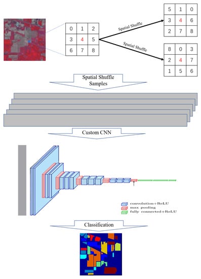
2.1. Spatial Shuffle

Due to the sensitivity of sensor photodetectors, HSI often exhibits phenomena of the “same object different spectrum” and “different objects same spectrum”, whereby each pixel may contain multiple land cover types, resulting in a scarcity of pure pixels. According to the first law of geography, the closer the distance between objects in space is, the greater their similarity is. Therefore, in a neighborhood, the distribution of surrounding pixels can be used to infer the attributes of the central pixel. For example, when all surrounding pixels belong to a certain land cover category, the probability that the central pixel also belongs to that category is higher. Based on this principle, this paper proposes the spatial shuffle strategy, which performs a random shuffle operation on the other neighboring pixels, except for the central pixel. Each operation forms a new spatial distribution, which may represent a potential land cover distribution pattern in the real world. By simulating as many potential distribution patterns as possible, the spatial combination rules between the central and neighboring pixels can be learned, thereby improving the deep model’s ability to describe and recognize spatial relationships in the neighborhood.
Specifically, for a neighborhood size of N × N, there are N × N − 1 pixels, excluding the central pixel. While keeping the position of the central pixel unchanged, a random shuffle is performed on the other N × N − 1 pixels, resulting in a new sequence as shown in Figure 1 below.
According to the rules of permutation and combination, it can be determined that when N = 3, there are a total of 8! = 40,320 potential patterns; meanwhile, when N = 5, there are a total of 24! = 6.2 × 10²³ potential patterns. Given M samples, theoretically, M × (N × N − 1)! samples can be generated, greatly expanding the number of samples. Although there is still a significant similarity between the samples, as a potential distribution pattern describing the real world, it can provide DL models with more learning capabilities.
However, it is impossible to generate M × (N × N − 1)! new samples in the actual application process, which will result in significant memory and graphics memory consumption. Therefore, this paper adopts a compromise-based solution, setting the total sample number for each category as K, assuming the category has M samples. K/M spatial shuffle operations are performed for each sample to ensure that the total number of samples for all categories is the same. This paper sets K = 100,000, and different K values can be chosen according to the actual situation.

2.2. Basic CNN

To test the effect of a spatial shuffle on classification performance, this paper outlines a basic CNN architecture of a convolution + BN + ReLU + Maxpooling design, without any structural optimization. The datasets used are Indian Pines (IP), Salinas Valley (SV), and University of Pavia (UP), which are widely used and publicly available, with 200, 204, and 103 effective bands, respectively. A sample with an N × N neighborhood and B bands is flattened into an image with B width and N × N after each spatial shuffle, thus transforming the three-dimensional cube of N × N × B into a two-dimensional image. For example, for the Indian Pines dataset, if N = 5, each sample is transformed into a 25 × 200 image for subsequent CNN network training.
As the band number in the three datasets is inconsistent, to maintain the original data dimensions, we designed the following three deep CNN networks in Table 1 for use with 5 × 5 patches:
The term Conv-BN-ReLU refers to each convolution layer that was followed by a batch normalization (BN) layer and rectified linear unit (ReLU) layer. Furthermore, (1 × 3) refers to the use of a convolution kernel size of 1 × 3, while 32 and 64 indicate the use of 32 and 64 convolution kernels, respectively. Similar to the VGG network, the network designed in this paper used a large number of small convolution kernels of 1 × 3 or 3 × 1 to achieve an equivalent field of view to that of a larger convolution kernel, while also reducing the number of parameters.
Taking the network for IP dataset as an example, with an input size of 25 × 200, we can see from the network structure that in Seq_1, four 1 × 3 convolution kernels were first used to extract features within the width dimension, reducing the dimensions to 25 × 192. Then, two 3 × 1 convolution kernels were used to convolve within the height dimension, reducing the dimensions to 21 × 192. After passing through the first 2 × 1 Maxpooling, the dimensions became 10 × 192. After two 3 × 1 convolution layers and 2 × 1 Maxpooling, the dimensions became 3 × 192. Finally, after passing through a 3 × 1 convolution layer and a 1 × 2 Maxpooling, the dimensions became 1 × 96. After Seq_2 to Seq_5, the dimensions became 1 × 45, 1 × 19, 1 × 6, and 1 × 1, respectively. After passing through the two fully connected layers in Seq_6 and Softmax, we received classnum classification results. The network structures of the other two datasets were essentially the same as that of Indian Pines, with some layers having different kernel numbers and convolutional layers due to differences in the number of bands.
From the above structure, we can see that the role of Seq_1 is to extract features from the height dimension, which can be understood as extracting spatial features of HSI in the neighborhood. The subsequent layers extracted spectral features of the sample. By the combination of spatial and spectral features, the category classification for each sample was formed.

3. Experiments and Results

3.1. Dataset

We used three publicly available HSI datasets, i.e., IP, SV, and UP, to demonstrate the effectiveness and generalization of the proposed method and compared its performance with commonly used methods. For each dataset, the values were first normalized to the range of 0–1. Then, for each class, 200 pixels and their surrounding 5 × 5 neighborhoods were randomly selected as the training samples, and the remaining pixels were used as the testing samples. These settings are the same as those in [37].
The IP dataset was obtained in northwestern Indiana, using the airborne visible infrared imaging spectrometer (AVIRIS) sensor. The original dataset had 224 bands, and after removing bands 104–108, 150–163, and 220 that contained voids or water vapor absorption, 220 bands were left. The spectral range was 0.4 to 2.5 μm. The spatial resolution was 20 m, and the image size was 145 × 145. The annotated ground truth contained 16 land cover categories, such as crops, forests, etc., with a total of 10,249 pixels, accounting for about half of the total pixels. However, the pixel number in seven categories was too small [38]; thus, this paper selected nine other categories for experimentation. The selected classes and their sample sizes are shown in Table 2 below.
The SV dataset was also collected using the AVIRIS sensor and located in the Salinas Valley, California. After removing 20 bands containing water vapor and noise, 204 bands were left with a data size of 512 × 217. The spatial resolution was 3.7 m. There were 16 land cover categories in the ground truth map, and specific land cover types and pixel numbers were in Table 3 as follows:
The UP dataset was obtained using the reflective optics system imaging spectrometer (ROSIS) sensor, covering part of the University of Pavia campus in the north of Italy. The noise and other unwanted bands were removed, and only 103 bands remained. The image size was 610 × 340 and the spatial resolution was 1.3 m. The spectral range was between 0.43 and 0.86 μm. About 20% of the pixels were labeled with ground truth, including various urban structures, soils, natural targets, and shadows. The specific number of pixels was in Table 4 as follows:

3.2. Parameter Settings

The software environment used for the experiments in this paper was Pytorch 1.0 and Python 3.6. The GPU hardware was NVIDIA TITAN XP, with a single card having 12 GB of memory. As the focus of this paper was not to design an exceptionally superior DL model, the model parameters were set based on experience using the Adam optimizer, and the learning rate was 0.0001. The batch size for the UP dataset was set to 1024, while for the SV and IP datasets, it was set to 512. The cross-entropy loss was used as the loss function.
For evaluating the effectiveness and accuracy of the proposed approach, various methods were used, including multinomial logistic regression (MLR) [39], support vector machines (SVM) [38], extreme learning machines (ELM) [40], random forests (RF) [41], CNN2D [34], and PPF [37]. The experiments were based on the same training and testing sets. MLR, SVM, and RF were implemented using the scikit-learn machine-learning library, while ELM was implemented using the scikit-elm library. Both CNN2D and PPF used a 5 × 5 neighborhood. For CNN2D, two 3 × 3 convolutional layers + BN layer + ReLU layer were used, followed by a fully connected layer for pixel classification, identical to [34]. The classification accuracy of various methods was evaluated using the overall accuracy (OA), average accuracy (AA), and Kappa coefficient. The OA was obtained by calculating the number of correctly classified pixels divided by the total number of pixels to be classified, while AA was the arithmetic mean of classification accuracies for each class. The Kappa coefficient reflects the consistency between the classified image and the ground truth image, with a range of −1 to 1, typically greater than 0.

3.3. Results on the IP Dataset

Figure 2 below shows the classification performance of various methods on the IP dataset, from which we can see that all methods perform well within Hay-windrowed and Grass/Trees classes. With the exception of MLR, other methods also had good results within the Woods class. However, traditional machine-learning methods (MLR, SVM, RF, ELM) performed poorly for other classes, with a lot of misclassifications. CNN2D, PPF, and the proposed method based on DL performed well for all classes, with the proposed method showing fewer misclassifications, indicating good classification ability.
The Table 5 below shows the classification accuracy of each method on each class, as well as the OA, AA, and Kappa. From the table, it can be seen that the accuracy of all methods is close to 100% for the Grass/Trees and Hay-windrowed classes. MLR performed poorly for other classes, resulting in the lowest overall accuracy and Kappa coefficient. The performances of SVM and RF were similar, while ELM and CNN2D performed better. The proposed method performed well for all classes, with the overall accuracy being 3.5% higher than the second-ranked PPF and about 35% higher than the worst MLR. All these results show that the proposed method demonstrated higher classification performance.

3.4. Results on the SV Dataset

Figure 3 below shows the classification thematic maps of each method on the SV dataset. It is obvious that the performance of each method is relatively poor on the Grapes-untrained and Vinyard vertical trellis classes, with the visual performance of the MLR method being the worst. However, the proposed method can provide a relatively clean thematic map. The CNN2D method had a larger misclassification rate on the Brocoli-gree-weeds-1 class, while other methods performed better for this class.
The Table 6 below shows the quantitative objective evaluation metrics of various methods for all classes. It is clear that the proposed method performed the best within almost all classes, with the overall accuracy (OA) being about 4% higher than the PPF method and approximately 12% higher than the worst-performing MLR method. The CNN2D method performed the worst on the Brocoli-gree-weeds-1 class, consistent with the visual judgment. The MLR method had the lowest accuracy for the Vinyard-untrained and Grapes-untrained classes, which directly lowered the overall accuracy. The proposed method had the highest OA, AA, and Kappa values, indicating that it had the highest classification ability and performance.

3.5. Results on the UP Dataset

The thematic map of the UP dataset is shown in Figure 4 below. The classification ability of various methods can be clearly seen from the misclassification of the three categories with the most pixels: Asphalt, Bare Soil, and Meadows. MLR had the most misclassifications, while the proposed method had the lowest level of misclassification, followed by PPF and CNN2D. The performance of the other machine-learning methods did not differ significantly.
The objective evaluation criteria in the Table 7 below show that the OA value of the MLR method was the lowest, and SVM performed the best among the four traditional machine-learning algorithms but was slightly inferior to the three DL-based methods. The proposed method can provide the highest classification accuracy for all categories, resulting in an overall accuracy of 99.3%, indicating that the proposed method showed the best classification ability for this dataset.

4. Discussion

4.1. Classification Ability with Less Samples

To compare the accuracy performance of various methods with fewer training samples, according to [34,37], this paper set the number of each type of training sample to 50, 100, 150, and 200, respectively, and used the same method to calculate the classification performance of various methods. The results are listed in Figure 5 below. Overall, with the increase in training samples, the classification performance of various methods on various datasets showed an upward trend, which is consistent with the general perception. SVM performed with a relative stability for several datasets and had a relatively excellent performance within traditional machine-learning algorithms. Due to the random generation of the weight matrix and the hidden layer threshold from input neurons to hidden neurons, ELM can cause the output matrix to be ill-conditioned when there are individual samples with large deviations among the training samples. The resulting network structure is unstable and has poor robustness, which reduces the classification performance of the network; hence, its performance was not very stable on these three datasets. The DL-based methods performed significantly better than traditional machine-learning-based methods for various training sample sizes across all three datasets. Moreover, the proposed method consistently showed the best classification ability.

4.2. Effects of Neighborhood Sizes

The role of the neighboring pixels is to provide spatial feature description ability for the center pixel. The larger the neighborhood is, the more spatial features can be extracted. Therefore, existing HSI classification methods based on spatial–spectral fusion mostly used larger neighborhoods. The earlier experiments in this paper used a neighborhood size of 5 × 5. To evaluate the impact of neighborhood size on classification accuracy, similar to [37], we compared three neighborhood sizes: 3 × 3, 5 × 5, and 7 × 7. As can be seen from Figure 6 below, with the neighborhood size increased, the classification performance improved significantly. However, the improvement intensity of 7 × 7 compared with 5 × 5 was not as large as that of 5 × 5 compared with 3 × 3, indicating that the improvement resulting from increasing the neighborhood size is limited. It should be pointed out that the CNN structure designed for the three datasets needed to be modified for the different neighborhood size. The larger the neighborhood is, the more layers the modified network will have, and the computation will be greater. Therefore, after balancing multiple factors, we chose a neighborhood size of 5 × 5 for the experiments and discussion.

4.3. Effects of Spatial Shuffle

After the operation of a spatial shuffle, a 5 × 5 neighborhood can produce up to 6.2 × 10²³ potential patterns, but it is impossible to produce so many samples within its practical application. Therefore, we randomly generated 100,000 samples for each class to increase the sample size. Intuitively, the more samples there are, the better the description of the real world is. However, this also increases the amount of computation. In order to evaluate the impact of the sample size on classification accuracy, we set four sample size levels: 50,000, 100,000, 200,000, and 300,000. Meanwhile, we also compared the performance without spatial shuffle, which means there were only 200 original training samples for each category. Using the same network structure, the final classification performance was evaluated, and the results are shown in Figure 7 below.
It can be seen that, without spatial shuffle, the classification performance on each dataset was significantly lower compared to the case with spatial shuffle. In particular, for the IP dataset, the classification accuracy was only around 0.65, while with spatial shuffle using 50,000 samples per class, the accuracy could reach around 0.97. The other two datasets also had an accuracy of around 0.9 without spatial shuffle, which was noticeably lower than with spatial shuffle using 50,000 samples per class. Without spatial shuffle, considering the experimental setup, there were only 200 samples per class for the IP and UP datasets, resulting in a total of 9 × 200 = 1800 samples. For the SV dataset, there was a total of 16 × 200 = 3200 samples. Training a CNN model on such small datasets easily leads to overfitting, which is the main reason for the low classification accuracy. However, by using spatial shuffle, the training samples can be expanded to 9 × 50,000 = 450,000 samples, or even more. This helps to mitigate the impact of overfitting and the significant improvement in classification accuracy further confirms this. With the increase in sample size, the classification performance for all three datasets improved. However, the degree of improvement generally tended to become saturated, not following a linear trend with the increase in sample size. Therefore, from a multi-factor balance perspective, our choice of 100,000 samples per class was reasonable. To further improve classification accuracy, future study will focus on optimizing the network structure.

5. Conclusions

Existing spatial–spectral fusion-based HSI classification methods mostly adopt larger neighborhoods to extract more spatial features to assist in the fine classification of each pixel. However, large neighborhoods may cause the problem of non-independence between the training set and testing set to some extent. Therefore, minimizing the neighborhood size may alleviate the above problem. This paper proposes a strategy called spatial shuffle, which randomly shuffles the positions of the pixels in the small neighborhood to simulate potential patterns that may exist in the real world. Through spatial shuffle, it is possible to quickly generate more simulated samples given a certain initial sample set. Experimental results have shown that this strategy effectively addresses the data requirement and overfitting issues in deep learning, leading to improved classification accuracy. The number of initial samples also has a decisive impact on the final classification accuracy. Although spatial shuffle allows for the generation of almost infinite samples to mimic the distribution patterns in the real world, the diversity of the initial samples may still be limited, which can restrict the simulated distribution patterns. However, even with this limitation, applying the spatial shuffle strategy and using the basic CNN model can achieve a consistently higher classification accuracy than traditional machine-learning methods and previously optimized CNN models. In addition, designing a deep-learning CNN model is not the focus of this paper; a simple CNN architecture based on convolution, batch normalization, and ReLU was constructed without any optimization measures, and the spatial shuffle samples were used for training. The experimental results indicate that the proposed method can effectively extract spatial and spectral features to improve the HSI classification performance. Different neighborhood window sizes can extract varying levels of spatial information, which also significantly affects the classification accuracy. By designing different network structures, it is possible to adapt to different sizes of neighborhood window sizes. Combined with the spatial shuffle strategy, it becomes possible to achieve classification accuracy comparable to previous studies using larger neighborhood window sizes even with smaller window sizes. This approach partially addresses the issue of overlapping and dependent training and testing samples during the training process. However, it should be noted that this paper only utilizes the basic, unoptimized CNN model and achieves remarkably high classification accuracy. Therefore, it is foreseeable that further improvement in classification performance can be achieved by optimizing the structure of the CNN model. Thus, future research will further explore the potential advantages of a spatial shuffle and optimize the constructed basic CNN architecture to further improve the accuracy of HSI classification.

Author Contributions

Methodology, Z.W. and J.L.; software, B.C.; investigation, Z.W., B.C. and J.L.; writing—original draft preparation, Z.W.; writing—review and editing, B.C. and J.L. All authors have read and agreed to the published version of the manuscript.

Funding

This research was supported in part by the 2022 Doctoral Research Initiation Fund of Hunan University of Chinese Medicine under Grant 0001036.

Data Availability Statement

The HSI datasets used in this paper are all public datasets.

Acknowledgments

All authors would like to thank the editors and reviewers for their detailed comments and suggestions.

Conflicts of Interest

The authors declare no conflict of interest.

References

  1. Gwon, Y.; Kim, D.; You, H.J.; Nam, S.H.; Kim, Y.D. A Standardized Procedure to Build a Spectral Library for Hazardous Chemicals Mixed in River Flow Using Hyperspectral Image. Remote Sens. 2023, 15, 477. [Google Scholar] [CrossRef]
  2. Shitharth, S.; Manoharan, H.; Alshareef, A.M.; Yafoz, A.; Alkhiri, H.; Mirza, O.M. Hyper spectral image classifications for monitoring harvests in agriculture using fly optimization algorithm. Comput. Electr. Eng. 2022, 103, 108400. [Google Scholar]
  3. Verma, R.K.; Sharma, L.K.; Lele, N. AVIRIS-NG hyperspectral data for biomass modeling: From ground plot selection to forest species recognition. J. Appl. Remote Sens. 2023, 17, 014522. [Google Scholar]
  4. Yang, H.Q.; Chen, C.W.; Ni, J.H.; Karekal, S. A hyperspectral evaluation approach for quantifying salt-induced weathering of sandstone. Sci. Total Environ. 2023, 885, 163886. [Google Scholar] [CrossRef]
  5. Calin, M.A.; Calin, A.C.; Nicolae, D.N. Application of airborne and spaceborne hyperspectral imaging techniques for atmospheric research: Past, present, and future. Appl. Spectrosc. Rev. 2021, 56, 289–323. [Google Scholar]
  6. Cui, J.; Yan, B.K.; Wang, R.S.; Tian, F.; Zhao, Y.J.; Liu, D.C.; Yang, S.M.; Shen, W. Regional-scale mineral mapping using ASTER VNIR/SWIR data and validation of reflectance and mineral map products using airborne hyperspectral CASI/SASI data. Int. J. Appl. Earth Obs. Geoinf. 2014, 33, 127–141. [Google Scholar]
  7. Kumar, V.; Ghosh, J. Camouflage detection using MWIR hyperspectral images. J. Indian Soc. Remote Sens. 2017, 45, 139–145. [Google Scholar] [CrossRef]
  8. Shimoni, M.; Haelterman, R.; Perneel, C. Hypersectral imaging for military and security applications: Combining myriad processing and sensing techniques. IEEE Geosci. Remote Sens. Mag. 2019, 7, 101–117. [Google Scholar] [CrossRef]
  9. Liu, J.J.; Wu, Z.B.; Li JPlaza, A.; Yuan, Y.H. Probabilistic-kernel collaborative representation for spatial–spectral hyper-spectral image classification. IEEE Trans. Geosci. Remote Sens. 2015, 54, 2371–2384. [Google Scholar] [CrossRef]
  10. Wu, L.; Huang, J.; Guo, M.S. Multidimensional Low-Rank Representation for Sparse Hyperspectral Unmixing. IEEE Geosci. Remote Sens. Lett. 2023, 20, 5502805. [Google Scholar] [CrossRef]
  11. Plaza, A.; Benediktsson, J.A.; Boardman, J.W.; Brazile, B.; Bruzzone, L.; Camps-Valls, G.; Chanussot, J.; Fauvel, M.; Gamba, P.; Gualtieri, A.; et al. Recent advances in techniques for hyperspectral image processing. Remote Sens. Environ. 2009, 113, S110–S122. [Google Scholar] [CrossRef]
  12. Li, J.; Marpu, P.R.; Plaza, A.; GenBioucas-Dias, J.M.; Benediktsson, J.A. Geralized composite kernel framework for hyperspectral image classification. IEEE Trans. Geosci. Remote Sens. 2013, 51, 4816–4829. [Google Scholar] [CrossRef]
  13. Zhang, Y.Q.; Cao, G.; Li, X.S.; Wang, B.S. Cascaded random forest for hyperspectral image classification. IEEE J. Sel. Top. Appl. Earth Observ. Remote Sens. 2018, 11, 1082–1094. [Google Scholar] [CrossRef]
  14. Gao, B.T.; Yu, L.F.; Ren, L.L.; Zhan, Z.Y.; Luo, Y.Q. Early Detection of Dendroctonus valens Infestation at Tree Level with a Hyperspectral UAV Image. Remote Sens. 2023, 15, 407. [Google Scholar] [CrossRef]
  15. Xia, J.S.; Du, P.J.; He, X.Y.; Chanussot, J. Hyperspectral remote sensing image classification based on rotation forest. IEEE Geosci. Remote Sens. Lett. 2013, 11, 239–243. [Google Scholar] [CrossRef] [Green Version]
  16. Hu, W.; Huang, Y.Y.; Wei, L.; Zhang, F.; Li, H.C. Deep convolutional neural networks for hyperspectral image classification. J. Sens. 2015, 2015, 258619. [Google Scholar] [CrossRef] [Green Version]
  17. Yang, X.F.; Ye, Y.M.; Li, X.T.; Lau, R.Y.K.; Zhang, X.F.; Huang, X.H. Hyperspectral image classification with deep learning models. IEEE Trans. Geosci. Remote Sens. 2018, 56, 5408–5423. [Google Scholar] [CrossRef]
  18. Ma, X.T.; Man, Q.X.; Yang, X.M.; Dong, P.L.; Yang, Z.L.; Wu, J.R.; Liu, C.H. Urban Feature Extraction within a Complex Urban Area with an Improved 3D-CNN Using Airborne Hyperspectral Data. Remote Sens. 2023, 15, 992. [Google Scholar] [CrossRef]
  19. Mou, L.; Ghamisi, P.; Zhu, X.X. Deep recurrent neural networks for hyperspectral image classification. IEEE Trans. Geosci. Remote Sens. 2017, 55, 3639–3655. [Google Scholar] [CrossRef] [Green Version]
  20. Liu, W.K.; Liu, B.; He, P.P.; Hu, Q.F.; Gao, K.L.; Li, H. Masked Graph Convolutional Network for Small Sample Classification of Hyperspectral Images. Remote Sens. 2023, 15, 1869. [Google Scholar] [CrossRef]
  21. Chen, Y.S.; Lin, Z.H.; Zhao, X.; Wang, G.; Gu, Y.F. Deep learning-based classification of hyperspectral data. IEEE J. Sel. Top. Appl. Earth Obs. Remote Sens. 2014, 7, 2094–2107. [Google Scholar] [CrossRef]
  22. Zhu, L.; Chen, Y.S.; Ghamisi, P.; Benediktsson, J.A. Generative adversarial networks for hyperspectral image classification. IEEE Trans. Geosci. Remote Sens. 2018, 56, 5046–5063. [Google Scholar] [CrossRef]
  23. Paoletti, M.E.; Haut, J.M.; Fernandez-Beltran, R.; Plaza, J.; Plaza, A.; Li, J.; Pla, F. Capsule networks for hyperspectral image classification. IEEE Trans. Geosci. Remote Sens. 2018, 57, 2145–2160. [Google Scholar] [CrossRef]
  24. Hang, R.L.; Liu, Q.S.; Hong, D.F.; Ghamisi, P. Cascaded recurrent neural networks for hyperspectral image classification. IEEE Trans. Geosci. Remote Sens. 2019, 57, 5384–5394. [Google Scholar] [CrossRef] [Green Version]
  25. Hong, D.F.; Gao, L.R.; Yao, J.; Zhang, B.; Plaza, A.; Chanussot, J. Graph convolutional networks for hyperspectral image classification. IEEE Trans. Geosci. Remote Sens. 2021, 59, 5966–5978. [Google Scholar] [CrossRef]
  26. Hong, D.; Han, Z.; Yao, J.; Gao, L.R.; Zhang, B.; Plaza, A.; Chanussot, J. SpectralFormer: Rethinking Hyperspectral Image Classification With Transformers. IEEE Trans. Geosci. Remote Sens. 2022, 60, 5518615. [Google Scholar] [CrossRef]
  27. Wu, H.; Prasad, S. Semi-supervised deep learning using pseudo labels for hyperspectral image classification. IEEE Trans. Image Process. 2018, 27, 1259–1270. [Google Scholar] [CrossRef] [PubMed]
  28. Huang, B.X.; Ge, L.Y.; Chen, G.; Radenkovic, M.; Wang, X.P.; Duan, J.M.; Pan, Z.K. Nonlocal graph theory based transductive learning for hyperspectral image classification. Pattern Recognit. 2021, 116, 107967. [Google Scholar] [CrossRef]
  29. Li, J.; Bioucas-dias, J.M.; Plaza, A. Semisupervised hyperspectral image classification using soft sparse multinomial logistic regression. IEEE Geosci. Remote Sens. Lett. 2013, 10, 318–322. [Google Scholar]
  30. Fang, B.; Li, Y.; Zhang, H.K.; Chan, J.C.W. Collaborative learning of lightweight convolutional neural network and deep clustering for hyperspectral image semi-supervised classification with limited training samples. ISPRS J. Photogramm. Remote Sens. 2020, 161, 164–178. [Google Scholar]
  31. Zhang, C.; Yue, J.; Qin, Q. Global prototypical network for few-shot hyperspectral image classification. IEEE J. Sel. Top. Appl. Earth Observ. Remote Sens. 2020, 13, 4748–4759. [Google Scholar] [CrossRef]
  32. Gao, K.L.; Liu, B.; Yu, X.C.; Qin, J.C.; Zhang, P.Q.; Tan, X. Deep relation network for hyperspectral image few-shot classification. Remote Sens. 2020, 12, 923. [Google Scholar] [CrossRef] [Green Version]
  33. Li, Z.K.; Liu, M.; Chen, Y.S.; Xu, Y.M.; Li, W.; Du, Q. Deep cross-domain few-shot learning for hyperspectral image classification. IEEE Trans. Geosci. Remote Sens. 2022, 60, 1–18. [Google Scholar] [CrossRef]
  34. Paoletti, M.E.; Haut, J.M.; Plaza, J.; Plaza, A. Deep learning classifers for hyperspectral imaging: A review. ISPRS J. Photogramm. Remote Sens. 2019, 158, 279–317. [Google Scholar] [CrossRef]
  35. Ghamisi, P.; Maggiori, E.; Li, S.T.; Souza, R.; Tarablaka, Y.; Moser, G.; De Giorgi, A.; Fang, L.Y.; Chen, Y.S.; Chi, M.M.; et al. New frontiers in spectral-spatial hyperspectral image classifcation: The latest advances based on mathematical morphology, markov random felds, segmentation, sparse representation, and deep learning. IEEE Geosci. Remote Sens. Mag. 2018, 6, 10–43. [Google Scholar]
  36. Yosinski, J.; Clune, J.; Bengio, Y.; Lipson, H. How transferable are features in deep neural networks? In Proceedings of the Advances in Neural Information Processing Systems, Montreal, QC, Canada, 8–13 December 2014; pp. 3320–3328. [Google Scholar]
  37. Li, W.; Wu, G.D.; Zhang, F.; Du, Q. Hyperspectral Image Classification Using Deep Pixel-Pair Features. IEEE Trans. Geosci. Remote Sens. 2017, 55, 844–853. [Google Scholar] [CrossRef]
  38. Melgani, F.; Bruzzone, L. Classification of hyperspectral remote sensing images with support vector machines. IEEE Trans. Geosci. Remote Sens. 2004, 42, 1778–1790. [Google Scholar] [CrossRef] [Green Version]
  39. Haut, J.; Paoletti, M.; Paz-Gallardo, A.; Plaza, J.; Plaza, A. Cloud implementation of logistic regression for hyperspectral image classifcation. In Proceedings of the 17th International Conference on Computational and Mathematical Methods in Science and Engineering, CMMSE, Rota, Spain, 4–8 July 2017; Vigo-Aguiar, J., Ed.; Springer: Berlin/Heidelberg, Germany, 2017; pp. 1063–2321. [Google Scholar]
  40. Li, J.; Zhao, X.; Li, Y.; Du, Q.; Xi, B.; Hu, J. Classifcation of hyperspectral imagery using a new fully convolutional neural network. IEEE Geosci. Remote Sens. Lett. 2018, 15, 292–296. [Google Scholar] [CrossRef]
  41. Ham, J.; Chen, Y.; Crawford, M.M.; Ghosh, J. Investigation of the random forest framework for classifcation of hyperspectral data. IEEE Trans. Geosci. Remote Sens. 2005, 43, 492–501. [Google Scholar] [CrossRef] [Green Version]
Figure 1. The overall schematic diagram of spatial shuffle scheme.
Remotesensing 15 03960 g001
Figure 2. Classification results of all methods on the IP dataset: (a) original HSI; (b) ground truth; (c) MLR; (d) SVM; (e) RF; (f) ELM; (g) CNN2D; (h) PPF; (i) proposed method.
Remotesensing 15 03960 g002aRemotesensing 15 03960 g002b
Figure 3. Classification results of all methods on the SV dataset: (a) original HSI; (b) ground truth; (c) MLR; (d) SVM; (e) RF; (f) ELM; (g) CNN2D; (h) PPF; (i) proposed method.
Remotesensing 15 03960 g003aRemotesensing 15 03960 g003b
Figure 4. Classification results of all methods on the UP dataset: (a) original HSI; (b) ground truth; (c) MLR; (d) SVM; (e) RF; (f) ELM; (g) CNN2D; (h) PPF; (i) proposed method.
Remotesensing 15 03960 g004aRemotesensing 15 03960 g004b
Figure 5. Classification performance of all methods using less samples on all datasets.
Remotesensing 15 03960 g005aRemotesensing 15 03960 g005b
Figure 6. Classification results of the proposed method using different neighborhood sizes on all datasets.
Remotesensing 15 03960 g006
Figure 7. Classification results of the proposed method using different number of samples per class on all datasets.
Remotesensing 15 03960 g007
Table 1. The basic CNN networks used for 5 × 5 patches.
IPSVUP
Seq_1Conv-BN-ReLU, (1 × 3), 32Conv-BN-ReLU, (1 × 3), 32Conv-BN-ReLU, (1 × 3), 32
Conv-BN-ReLU, (1 × 3), 32Conv-BN-ReLU, (1 × 3), 32Conv-BN-ReLU, (1 × 3), 32
Maxpool_2 × 1Maxpool_2 × 1Maxpool_2 × 1
Conv-BN-ReLU, (3 × 1), 32Conv-BN-ReLU, (3 × 1), 32Conv-BN-ReLU, (3 × 1), 32
Maxpool_2 × 1Maxpool_2 × 1Maxpool_2 × 1
Conv-BN-ReLU, (3 × 1), 32Conv-BN-ReLU, (3 × 1), 32Conv-BN-ReLU, (3 × 1), 32
Maxpool_1 × 2Maxpool_1 × 2Maxpool_1 × 2
Seq_2Conv-BN-ReLU, (1 × 3), 32Conv-BN-ReLU, (1 × 3), 32Conv-BN-ReLU, (1 × 3), 32
Conv-BN-ReLU, (1 × 3), 32Conv-BN-ReLU, (1 × 3), 32Conv-BN-ReLU, (1 × 3), 32
Maxpool_1 × 2Maxpool_1 × 2Maxpool_1 × 2
Seq_3Conv-BN-ReLU, (1 × 3), 64Conv-BN-ReLU, (1 × 3), 64Conv-BN-ReLU, (1 × 3), 64
Conv-BN-ReLU, (1 × 3), 64Conv-BN-ReLU, (1 × 3), 64Conv-BN-ReLU, (1 × 3), 64
Conv-BN-ReLU, (1 × 3), 64Conv-BN-ReLU, (1 × 3), 64Maxpool_1 × 2
Maxpool_1 × 2Maxpool_1 × 2
Seq_4Conv-BN-ReLU, (1 × 3), 64Conv-BN-ReLU, (1 × 3), 64Conv-BN-ReLU, (1 × 3), 64
Conv-BN-ReLU, (1 × 3), 64Conv-BN-ReLU, (1 × 3), 64Conv-BN-ReLU, (1 × 3), 64
Maxpool_1 × 2Maxpool_1 × 2
Seq_5Conv-BN-ReLU, (1 × 3), 64Conv-BN-ReLU, (1 × 3), 64
Conv-BN-ReLU, (1 × 3), 64Conv-BN-ReLU, (1 × 3), 64
Conv-BN-ReLU, (1 × 3), 64
Seq_6FC-64FC-64FC-64
FC-classnumFC-classnumFC-classnum
Table 2. The samples chosen from IP dataset.
No.Class NameTraining NumTesting NumAll Num
0Background--10,776
1Alfalfa--46
2Corn-notill20012281428
3Corn-min200630830
4Corn--237
5Grass/Pasture200283483
6Grass/Trees200530730
7Grass/pasture-mowed--28
8Hay-windrowed200278478
9Oats--20
10Soybeans-notill200772972
11Soybeans-min20022552455
12Soybean-clean200393593
13Wheat--205
14Woods20010651265
15Bldg-Grass-Tree-Drives--386
16Stone-steel towers--93
Total1800743421,025
Table 3. The samples chosen from SV dataset.
No.Class NameTraining NumTesting NumAll Num
0Background--56,975
1Brocoli-gree-weeds-120018092009
2Brocoli-gree-weeds-220035263726
3Fallow20017761976
4Fallow-rough-plow20011941394
5Fallow-smooth20024782678
6Stubble20037593959
7Celery20033793579
8Grapes-untrained20011,07111,271
9Soil-vinyard-develop20060036203
10Corn-senesced-green-weeds20030783278
11Lettuce-romaine-4wk2008681068
12Lettuce-romaine-5wk20017271927
13Lettuce-romaine-6wk200716916
14Lettuce-romaine-7wk2008701070
15Vinyard-untrained20070687268
16Vinyard-vertical-trellis20016071807
Total320050,929111,104
Table 4. The samples chosen from UP dataset.
No.Class NameTraining NumTesting NumAll Num
0Background--164,624
1Asphalt20064316631
2Meadows20018,44918,649
3Gravel20018992099
4Trees20028643064
5Painted metal sheets20011451345
6Bare Soil20048295029
7Bitumen20011301330
8Self-Blocking Bricks20034823682
9Shadows200747947
Total180040,976207,400
Table 5. The classification performance on the IP dataset.
MLRSVMRFELMCNN2DPPFProposed
Corn-notill42.5963.8461.9778.3488.0397.3198.53
Corn-min37.4466.2068.6381.9896.1995.4999.65
Grass/Pasture70.5295.5292.1695.1598.1399.2599.25
Grass/Trees95.28100.0098.11100.00100.0099.81100.00
Hay-windrowed100.00100.0099.64100.00100.00100.00100.00
Soybeans-notill62.5872.1084.2285.0195.3195.7097.52
Soybeans-min62.0063.7664.3561.6876.2386.9496.25
Soybean-clean36.6484.4879.3993.6499.75100.00100.00
Woods87.7998.1296.6298.40100.0099.8199.72
OA63.4276.1276.6881.0489.9394.7398.26
AA66.0982.6782.7988.2494.8597.1598.99
Kappa0.56470.71840.72590.77760.88100.93710.9792
Table 6. The classification performance on the SV dataset.
MLRSVMRFELMCNN2DPPFProposed
Brocoli-gree-weeds-197.8298.8599.4399.8362.41100100
Brocoli-gree-weeds-297.8299.8999.7499.83100100100
Fallow92.0699.3899.0497.7599.9499.7799.94
Fallow-rough-plow99.0899.599.4199.1610099.6699.92
Fallow-smooth97.798.1497.5498.7197.5898.3599.56
Stubble99.4699.9299.8199.8710010099.97
Celery99.499.9199.2999.7699.7699.9799.97
Grapes-untrained70.4485.0361.6683.8389.5983.9295.71
Soil-vinyard-develop96.2199.4898.8399.9299.9299.999.98
Corn-senesced-green-weeds85.4494.3788.2894.3794.6498.5198.84
Lettuce-romaine-4wk92.4497.5293.1594.9299.4110099.65
Lettuce-romaine-5wk99.6499.8297.6399.2399.94100100
Lettuce-romaine-6wk98.8699.7198.159910099.57100
Lettuce-romaine-7wk91.1998.2494.8394.3699.6599.2999.18
Vinyard-untrained62.7869.3669.6469.4173.9385.8294.33
Vinyard-vertical-trellis91.0898.7698.2798.6999.7299.4599.93
OA85.8491.848691.4792.3694.3198.16
AA91.9696.1293.4295.5494.7897.7699.19
Kappa0.84170.90860.84410.90440.91420.93640.9794
Table 7. The classification performance on the UP dataset.
MLRSVMRFELMCNN2DPPFProposed
Asphalt73.5588.9481.3262.0896.0198.299.64
Meadows75.7793.7278.491.290.4697.7899.53
Gravel76.9585.2376.8981.6695.7391.6797.78
Trees93.0696.0294.9695.1497.5796.5597.75
Painted metal sheets99.2199.6599.5699.4810099.91100
Bare Soil73.4990.4382.6183.3598.9297.5499.88
Bitumen89.1291.5990.3591.9598.7694.4298.32
Self-Blocking Bricks74.7383.4678.8968.1290.0992.1998.71
Shadows99.8710010099.8710099.87100
OA77.8391.6881.8683.9193.7696.9799.3
AA83.9792.128785.8796.3996.4699.07
Kappa0.71520.88980.76620.78880.91810.95950.9906
Disclaimer/Publisher’s Note: The statements, opinions and data contained in all publications are solely those of the individual author(s) and contributor(s) and not of MDPI and/or the editor(s). MDPI and/or the editor(s) disclaim responsibility for any injury to people or property resulting from any ideas, methods, instructions or products referred to in the content.

