Article

Estimating Plant Nitrogen by Developing an Accurate Correlation between VNIR-Only Vegetation Indexes and the Normalized Difference Nitrogen Index

Computer Engineering, TED University, Ankara 06420, Turkey
Remote Sens. 2023, 15(15), 3898; https://doi.org/10.3390/rs15153898
Submission received: 16 July 2023 / Revised: 2 August 2023 / Accepted: 4 August 2023 / Published: 7 August 2023

Abstract

:
Nitrogen is crucial for plant physiology due to the fact that plants consume a significant amount of nitrogen during the development period. Nitrogen supports the root, leaf, stem, branch, shoot and fruit development of plants. At the same time, it also increases flowering. To monitor the vegetation nitrogen concentration, one of the best indicators developed in the literature is the Normalized Difference Nitrogen Index (NDNI), which is based on the usage of the spectral bands of 1510 and 1680 nm from the Short-Wave Infrared (SWIR) region of the electromagnetic spectrum. However, the majority of remote sensing sensors, like cameras and/or satellites, do not have an SWIR sensor due to high costs. Many vegetation indexes, like NDVI, EVI and MNLI, have also been developed in the VNIR region to monitor the greenness and health of the crops. However, these indexes are not very well correlated to the nitrogen content. Therefore, in this study, a novel method is developed which transforms the estimated VNIR band indexes to NDNI by using a regression method between a group of VNIR indexes and NDNI. Training is employed by using VNIR band indexes as the input and NDNI as the output, both of which are calculated from the same location. After training, an overall correlation of 0.93 was achieved. Therefore, by using only VNIR band sensors, it is possible to estimate the nitrogen content of the plant with high accuracy.

1. Introduction

Numerous physiological activities in leaves, including photosynthesis, respiration, and transpiration, are primarily regulated by nitrogen [1,2,3]. Nitrogen is also closely related to chlorophyll concentration, light utilization efficiency, and net crop production [4,5,6]. In addition to frequently being a limiting factor for plant growth [7,8,9], nitrogen is a crucial input in the cycle of ecological processes [10,11]. Leaf nitrogen content has also been suggested as one of the crucial biodiversity variables for the monitoring of the progress towards the Aichi Biodiversity Targets by the remote sensing and ecology communities, who acknowledge the significant role of leaf nitrogen in biodiversity and ecosystem functioning [12,13].
Despite being a relatively minor element of leaves (up to 6.5–7%), nitrogen has been reliably recovered using leaf- and canopy-level hyperspectral data [14,15]. By offering contiguous, narrow spectral band data, hyperspectral data can be used to identify the nitrogen’s small absorption properties. Compared to the conventional destructive sample procedures, this provides an effective and economical way to assess leaf nitrogen. The spectra from leaf powder, dry leaves, and fresh leaves were employed in previous research on the determination of nitrogen concentration in vegetation, as well as estimates at the canopy level [16,17,18]. The mask of the significant water absorption [17,19], the confounding effects coming from the canopy structure, illumination/viewing geometry, and background [20,21], and other obstacles make it difficult to retrieve nitrogen at the canopy level.
Based on the previous studies conducted in the literature to estimate the nitrogen content of the plant, the contributions of this study are as follows:
-
Using the radiance values provided by Hyperion data directly without applying any atmospheric correction.
-
Developing a proper deep model which transforms VNIR-only vegetation indexes to NDNI with a high correlation.
-
Removing the necessity to have high-cost special cameras like SWIR to measure the nitrogen content of the crop.
-
Enabling the farmers to follow the nitrogen content of the crop progressively and decide when to/not to fertilize.

2. Related Work

To improve the nitrogen content estimation performance, numerous methods have been employed. One method is spectral transformation, which includes employing first/second derivatives and reflectance log transformation [22,23]. There are also other studies, which include continuum removal [17,24], water removal [25,26], and wavelet analysis [27]. Numerous studies have been proposed to estimate the nitrogen content over forests [18,23,28,29,30], grasslands [31,32,33], and crop ecosystems [34,35,36]. A variety of artificial intelligence techniques, including support vector regression, neural networks, and Bayesian model averaging [32,36,37], as well as traditional regression techniques like stepwise multiple linear regression and partial least square regression, are used to retrieve nitrogen concentration.
Vegetation indices are one of the simplest and most popular empirical methodologies for estimating the biochemical content of leaves, including the nitrogen level. The main sources of nitrogen in leaf cells are proteins and chlorophylls [38]. Since there is a strong correlation between nitrogen and chlorophyll in a variety of species [1,2,39], nitrogen has been estimated using vegetation indices which are proposed and used for chlorophyll estimation [40]. For measuring chlorophyll, spectral wavelengths around 550 nm and 700 nm, as well as the red-edge area (680–780 nm), have been used [35,41], leading to a significant variety of indices [42,43,44]. In contrast to chlorophyll, there are fewer studies that offer particular indices for nitrogen estimate; the majority of these indices were established for crops [45,46,47,48], while just a small number were developed for forests [49].
Given that canopy structure is the primary cause of changes in canopy reflectance, the calculation of foliar nitrogen using canopy spectral data is complicated. According to the study in [7], the NIR reflectance (800–850 nm) and canopy foliar mass-based nitrogen concentration (%N) have a significant association that can be utilized to predict nitrogen, and in [50] the researchers pointed out the association between NIR reflectance and canopy structure. The study in [51] suggested that the biological associations between nitrogen and structural characteristics that affect NIR scattering and reflectance served as the foundation for their ideas. Additionally, in [14,52], scientists indicated that the canopy structure and leaf characteristics may co-vary among plant functional types, contradicting the study in [53], which claimed that the %N-NIR correlation is inherently false.
The purpose of the study in [54] was to assess how well 32 vegetation indicators collected from airborne hyperspectral imaging performed when used to calculate canopy foliar nitrogen in a mixed temperate forest. For comparison, the widely used partial least squares regression was carried out. These vegetation indicators can be divided into three groups, most of which are connected to the biochemical and structural characteristics of vegetation (e.g., nitrogen, chlorophyll, and leaf area index (LAI)). The nitrogen indicators are selected based on how nitrogen absorption characteristics’ physical underpinnings affect canopy reflectance. The biological connections between nitrogen, chlorophyll, and canopy structure were used to justify the inclusion of the structural and chlorophyll indices in this study. Nitrogen (N) losses and the ensuing environmental issues are what define the production of vegetable crops [55,56,57]. The most frequent environmental issues include nitrous oxide (N2O) emissions, ground and surface water contamination, and the eutrophication of surface waters [58,59]. These issues are frequently a result of the extensive use of N fertilizer [60], which typically exceeds the requirement of the crops [57,61,62], which is performed to ensure optimal growth and production. In order to decrease N contamination of water bodies by intensive vegetable production, it is necessary to understand crop nitrogen requirements and match crop demand with nitrogen supply [57,63,64].
There are numerous techniques available for tracking crop nitrogen status [57,65]. Leaf nutritional analysis is a common method, but it is time-consuming and labor-intensive in the lab, and it typically cannot quantify the temporal and geographical variability of nitrogen status [66,67]. These are significant drawbacks, since it is much easier to match the supply of nitrogen to crop requirements when one is aware of the temporal and spatial variability of crop nitrogen status [68].
Optical sensors are tools that quickly, accurately, and nondestructively monitor the crop’s nitrogen status in the field [57,69]. They make it possible to regularly evaluate a crop and evaluate spatial variability. Canopy reflectance sensors, which are among the proximal optical sensors, have two highly advantageous characteristics in that they can monitor huge portions of a crop while they are in motion [70]. Field crops’ nitrogen status can be evaluated via measures of crop reflectance [65]. These measures are based on the differential reflection of light wavelengths [57], which, depending on crop nitrogen status [69], are absorbed and reflected by the crop in varying amounts. Typically, red, green, and near-infrared light wavelengths are employed for nitrogen estimation [65]. Recently, the red edge has been suggested as a solution for nitrogen estimation of the red band’s apparent saturation [71,72].
The nitrogen nutrition index (NNI) [67,73] is another commonly utilized strategy. The critical crop nitrogen content [74,75] is the lowest crop nitrogen content required for non-limiting growth, and it is used to calculate the NNI by dividing the actual crop nitrogen content by it. Any variation from 1 indicates either excess nitrogen (i.e., NNI > 1) or insufficient nitrogen (i.e., NNI1) crop status, with values of NNI equal to 1 indicating adequate nitrogen feeding [76].
Due to the high cost of SWIR band sensors, a regression-based method should be developed which maps the VNIR band indexes to SWIR band indexes. The majority of studies have been performed on cereal crops [77,78] like wheat [12,79] and rice [80,81,82]; very few have been carried out on vegetable crops like sweet pepper.
In [83], the crop nitrogen status of sweet pepper was estimated using eight vegetation indices that were computed from canopy reflectance data taken with two separate proximate sensors. First, crop NNI calibration regression models were fitted for each vegetation index. Second, a different dataset was used to validate these regression equations. Thirdly, sufficient values for each vegetative index for optimal nitrogen nutrition, for the main phenological stages of sweet pepper crops, were obtained utilizing the validated equations between vegetation indices and crop NNI.
The findings of the study [84] supported the use of the normalized difference vegetation index (NDVI) as a useful tool for determining the nitrogen status of cotton leaves at various growth stages. Using vegetation indices, the study in [85] calculated the nitrogen nutrition index (NNI), canopy nitrogen density (CND), and leaf nitrogen content of winter wheat over the course of the entire growth period. This study demonstrated that the correlations between each nitrogen index and the Vogelmann red-edge index (VOG), simple ratio pigment index (SRPI), modified red-edge simple ratio index, and red-edge position based on the linear interpolation method (REPliner) were not significantly influenced by growth period, and the estimation model R2 for CND was higher than 81%. The estimation model’s accuracy was higher than NNI; however, it would become saturated if CND was calculated using just one vegetation index. The red-edge chlorophyll index, CIred-edge, was demonstrated by [86] to be responsive to the canopy structure. The correlation between the nitrogen content of cotton leaves and several spectral ratio measures was examined in [87], who also conducted a cluster analysis based on prediction accuracy and overall accuracy.
The ratio of the red-edge position to the near-infrared band was shown to have a pretty high prediction accuracy and overall accuracy. The estimation of the winter wheat spectral index was investigated by [88] in a variety of environments, seasons, varieties, and growth stages. According to their findings, the growth stage had a significant impact on the performance of various vegetation indices and the choice of a sensitive wavelength for plant nitrogen concentration (PNC) estimation. The simple ratio of reflectivity at 370 nm and 400 nm (R370/R400) displayed the most consistent estimation accuracy in an indoor experiment (R2 = 0.58) and field experiment (R2 = 0.51). According to the studies, there are obvious changes in the relevant spectral index for different crops, or for various kinds and ecological zones of the same crop, when employing the spectral index to estimate crop nitrogen [89,90].
Additionally, compared to employing sensitive spectral features alone or vegetation indexes, modeling techniques like deep machine learning can produce greater prediction effects [91]. These techniques can also be used to monitor agricultural nutrients and growth indicators [92,93,94]. Support vector machine regression (SVR) was shown to be the most effective method for assessing crop nutrient contents in [95], which evaluated artificial neural network and SVR methods. The authors proposed that the creation of models with large sample sizes is appropriate for an artificial neural network. The hyperspectral reflectance of leaves was used in [90] to study the generalized partial least-squares regression (PLSR) model, and this approach was successful in retrieving leaf nitrogen concentration (r = 0.85).
The study in [96] is based on data for two types of drip-irrigated cotton at various growth stages from April 2019 to September 2020. The data include canopy nitrogen density (CND) and leaf nitrogen concentration (LNC) values. Pearson’s correlation analysis was used to determine which of the thirty hyperspectral vegetation indexes and the two nitrogen indexes (LNC and CND) that were used in the three modeling techniques of simple multiple linear regression (MLR), PLSR, and support vector regression (SVR) were relatively stable. The models were employed to investigate the possibility of measuring the nitrogen nutrient status of cotton in each growth period based on a multi-vegetation index in order to give a theoretical background for the application of remote sensing technology in cotton nutrition monitoring and diagnostics.
The nitrogen attitude of paddy rice was studied in [97], including plant nitrogen content (PNC), leaf nitrogen content (LNC), plant nitrogen accumulation (PNA), and leaf nitrogen accumulation (LNA). The data used in this study were collected by using a hyperspectral camera integrated to an unmanned aerial vehicle (UAV). The results handled in this study report that the correlation between the nitrogen traits and biochemical traits, canopy chlorophyll content, leaf chlorophyll content and aboveground biomass, depend on the growth stage of the crop.
The study in [98] fused the information from different sensors and developed new spectral indices based on a coverage-adjustment and estimated the content of leaf nitrogen of maize in different stages of the growth. According to the results, CASIs perform better than the traditional vegetation indices.
According to the results of the study in [99], which developed an estimation method of potato nitrogen, combining the visible light vegetation indexes and plant morphological properties provides a better estimation of nitrogen, since by using multiple linear regression methods it achieves a 0.79 R2 score.
Researchers developed a new method in [100] which extracts the leaf region from the color images and computes the color similarity between the extracted leaf with some predefined color information. In particular, a green color intensity was used for the reference of nitrogen content. The proposed method was tested on a Spinacia oleracea dataset and results showed that there exists a high correlation between the laboratory analysis and the analysis of the color images.

3. Materials and Methods

Image data of the Hyperion sensor were used in this study. As a push-broom hyperspectral instrument, Hyperion is housed on the EO-1 satellite, which is depicted in Figure 1.
With a 10 nm bandwidth spanning from 357 nm to 2576 nm, it collects 220 different spectral channels. All bands have a spatial resolution of (30 × 30) m2. The VNIR band, SWIR band, and VNIR-SWIR band indices can all be estimated from the same image data because Hyperion includes both the VNIR and SWIR bands. There is no need for a geometric correction because the Hyperion images have already been rectified geometrically. In addition, no atmospheric correction is applied to the data. This is due to the fact that atmospheric correction tools are not free to use, so, bring high financial costs. In addition, they cannot achieve a perfect correction, which produces incorrect reflectance values among the pixels and affects the results negatively. The properties of the Hyperion sensor are given in Table 1.
Different test images were collected from Hyperion data on the Harran region based in the south-west of Turkey. Google Earth and Earth explorer views of Harran and the Hyperion image are shown in Figure 2.
The Harran Plain is a region that starts from the southeast of the city of Şanlıurfa and extends to the Syrian border. It is a plain with very fertile soil. It is located between the 36°43′–37°08′N parallels and 38°57′–39°55′E meridians in the Upper Mesopotamian area of Şanlıurfa province.
In the main, corn and cotton farming is carried out. In the Harran Plain, under the influence of the Mediterranean climate, the continental climate is dominant. Winters are cold and rainy, and summers are very hot and dry. Annual precipitation is 365 mm, annual evaporation is 1848 mm, and annual average temperature is 17.2 °C.
The Hyperion image downloaded from Earth Explorer covers roughly 900 km2, which is both required and sufficient to investigate the reliability of the proposed method. The QGIS Geographic Information Software Tool was used to determine the area of the Hyperion images [102]. Figure 3 shows the image data taken from the Harran region, in which a large amount of corn, cotton and wheat planting is undertaken by farmers. The image acquisition time was 8 August 2016, when the crop was dense and mature. The image’s latitude and longitude values and the scale of the map are given on the figure as well.
Figure 4 shows a drone camera view and a ground image of a region from Harran taken in July 2019.
In the Harran region, to show the vegetation density and the spreading over the area, an NDVI estimation was first applied. The Hyperion image and the resulting NDVI index map are shown in Figure 5. The Hyperion image has a spatial resolution of 3241 × 1241, totaling 4,022,081 pixels, where 2,859,262 pixels are the black regions surrounding the target region. Therefore, the vegetation index analysis is implemented on 1,162,819 pixels. Each pixel corresponds to 30 × 30 m2 ground area. By recalling that NDVI values can be changed from −1 to 1, in Table 2 it can be seen that the number of pixels with a high NDVI value, like >0.75, was lower, relatively speaking. An important reason for this is the ground spatial resolution of the Hyperion sensor, in which one pixel covers 30 × 30 m2. This is, relatively, a large area in which spectral mixing occurs, and therefore the spectra of soil, water and vegetation is mixed, which may reduce the NDVI indices [104]. Nonetheless, the data are powerful and exhibit a good distribution, which enables an accurate analysis of vegetation indices.
To increase the accuracy, the pixels with NDVI values higher than 0.2 were taken into account. This is due to the typical vegetation pixel having an NDVI greater than 0.2.
The study in [105] states that NDNI can be used effectively for the estimation of the nitrogen content of the vegetation. Since, in this study, we develop a deep model which established a correlation between VNIR band vegetation indices and NDNI, the most important vegetation indices which hold information about the nitrogen content of the plants were estimated. These indices are NDVI [106], GNDVI [107], EVI [108], GOSAVI [109], GSAVI [109], MCARI2 [110], and VREI2 [111]. To establish the correlation, NDNI [112] was estimated as well. Table 3 shows the corresponding indices, the bands or wavelengths, and the equations which were used to estimate them.
The black regions on the Hyperion data were excluded first. Then, each vegetation index was estimated for the pixels left. N was the number of pixels in each index map, and a vector of index values was created, as shown in Equation (1), where M a p v i was the index map of the corresponding vegetation index and i n d e x i was the estimated index value at pixel i.
M a p v i = [ i n d e x 1 , i n d e x 2 i n d e x N ]
Then, new index data were created, as shown in Equation (2), where I v . i . a b was the estimated index for the (b). pixel of vegetation index (a). (i.e., 3rd pixel of NDVI map).
d a t a = I v . i . 11 I v . i . 1 N I v . i . M 1 I v . i . M N
Since this study uses 7 vegetation indices from the VNIR region, a total of 7 M a p v i were created at the beginning. Therefore, the size of the data matrix was (7 × 1,162,819). After handling the data matrix, a further analysis was carried out.
-
Due to the division by 0, some index values were calculated as infinite and/or NaN. Therefore, those kinds of pixels were found and the corresponding column was deleted.
-
Another analysis was also carried out for the pixels with an abnormally large vegetation index. Therefore, the index values which had an absolute value above 5 were also deleted from the data.
-
Finally, 1,113,529 pixel values were used, and to normalize the effect of the environment at the time of the capturing, each index row in the data was normalized between −1 and 1. To normalize the data, the normalize function of Matlab was used with a ‘range’ parameter.
Similarly, the above operations were also applied on the NDNI Map. Finally, the input data had the shape of (7 × 1113529) and the output data had (1 × 1113529).
To train a model which matches the input data to the output data, Matlab deep learning toolbox [113] was used. By using this tool, a deep neural network was designed with 4 dense (hidden) layers, each with 25 neurons. Figure 6 shows the designed neural network. The number of input neurons was 7 due to the shape of the input data and 1 for output, hence that was the NDNI index value.
Data were split into train, validation, and test datasets with the default ratio of 0.7:0.15:0.15. The number of epochs was set as 1000. Training function and adaption learning functions were set as TRAINLM (Levenberg–Marquardt) and LEARNGDM. LEARNGDM is a gradient descent algorithm with momentum. The cost can be pushed farther to go around a saddle point by adding a momentum element to the gradient descent, even if the current gradient is insignificant. The performance function is MSE. Training was carried out on CPU on a Windows PC with 8 GB Ram and an 11th Gen Intel(R) Core(TM) i7-1165G7 @ 2.80 GHz processor. The reason not to use GPU was that in Matlab, the TRAINLM function is not supported.
The Levenberg–Marquardt [114] technique, which was developed for minimizing functions that are sums of squares of nonlinear functions, is derived from Newton’s method [115]. The Levenberg–Marquardt algorithm is designed to minimize sum-of-square error functions of the form (3). In (3), e r r k is the error in the kth instance and e r r is a vector with element at k. A Taylor series can be used to expand the error vector to first order if the difference between the old and new weight vectors is modest.
E = 1 2 k ( e r r k ) 2 = 1 2 e r r 2
e r r j + i = e r r j + e r r k w i ( w j + 1 w j )
As a result, the error function can be expressed as
E = 1 2 e r r ( j ) + e r r k w i ( w j + 1 w j ) 2
After minimizing the error function with respect to the updated weight vector, (6) can be written.
w j + 1 = w j ( Z T Z ) 1 Z T e r r ( j )
where
Z k i e r r k w i
Since the Hessian for the sum-of-square error function is as shown in (8),
H i j = 2 E w i w j + { ( e r r k w i ) e r r k w i + e r r k ( 2 e r r k w i w i ) }
By ignoring the second term, Hessian can be written as:
H = Z T Z
For nonlinear networks, updating the weights therefore entails the inverse Hessian. Since the Hessian is based on first order derivatives with respect to the network weights, which can be easily handled by back propagation, it can be calculated rather quickly. Although iterative application of the updating formula to reduce the error function is an option, this may provide a step size that is too big, invalidating the linear approximation that the method is based on.
The Levenberg–Marquardt approach minimizes the error function while maintaining a small step size to guarantee the accuracy of the linear approximation. Utilizing a form’s customized error function allows for this.
E = 1 2 e r r ( j ) + e r r k w i ( w j + 1 w j ) 2 + α ( w j + 1 w j ) 2
where α is a parameter adjusting the step size. When the modified error is minimized with respect to w j + 1 , (11) is handled.
w j + 1 = w j ( Z T Z + α I ) 1 Z T e ( j )
With very large values of α , Levenberg–Marquardt approaches standard gradient descent, whereas for very small values of α it approaches the Newton method.
This study aims to investigate the relation between VNIR-only vegetation indexes and NDNI. For that purpose, linear regression was employed by using a deep neural network. Linear regression can be explained as follows:
Y = a + b X + ε
where
a = y x 2 x x y n ( x 2 ) x 2
b = n x y x y n ( x 2 ) x 2
In Equation (12), Y is the dependent (outcome) variable, a is y-intercept, b is the slope of the regression line, X is the independent variable, and ε is the error term. The calculation of linear regression includes 3 steps:
  • First, the values of formula components a and b are found by using x , y , x y , and x 2 ;
  • Then, the values derived in the first step are substituted into a and b ;
  • Finally, a and b values are used with the formula Y = a + b X + ɛ to establish the linear relationship between X and Y variables.
Since a deep neural network is used in this study, the calculation is performed by the neural network tool defined in Matlab and linear regression is employed.

4. Results

Regression and loss plots are given in Figure 7 and Figure 8, respectively, for training, validation, test, and overall data. The R2 values for test and validation data are above 0.91 and 0.93, respectively, which is very promising. Similarly, the MSE loss values are all below 10−4. The best validation loss score is 7.01 × 10⁻⁵, which means 70 over 1 million. As can be observed from Figure 7, although the number is low, there are some outlier values which do not fit the regression line. They are the points which are far from the regression line and whose correlation error is generally high. Therefore, the outliers affect the regression score negatively. Those points are generally the anomaly points/regions in the flat areas. The best validation score was achieved at epoch 124, and therefore the training was stopped at epoch 130.
The regression equations between input and output handled for training, validation, test and all data are given in Table 4.
Various machine learning methods based on regression were also trained and tested. In Table 5, the best regression scores handled are given for comparison with the proposed method. It can be obviously seen from the table that the proposed method achieves the best and superior results compared to all other methods.

Ablation Study

In this study, a deep neural network was employed to investigate the correlation between VNIR-Only vegetation indexes and the NDNI index. For this purpose, various combinations of different networks on normalized and/or unnormalized data were tried. Figure 9 shows the regression results when the depth of the network was reduced to two deep layers and data were normalized. Even if test score was improved a bit, validation and all data scores were not good as the proposed network.
Figure 10 shows the regression result for two deep layers on unnormalized data, which were worse and unbalanced among training, validation and test data. Therefore, when the network is not deep enough, normalization of the data is crucial.
When the depth of the network is kept and data are not normalized, similar regression results to the proposed network can be seen (Figure 11). However, the results are still a bit better when the data are normalized. In addition, when the data are normalized, the depth of the network can be reduced to two with very little and tolerable reduction in accuracy. In this way, the response time of the network to new data can be reduced, which is crucial for near real-time and/or real-time applications.
Various neural networks with different numbers of deep layers and neurons were trained with the normalized data, and the obtained regression scores for training, validation, test, and all data are given in Table 6. The best scores are colored in red and the second-best scores are colored in blue. As (#L, #N) shows the number of deep layers and neurons at each deep layer, (4,15) includes the three best scores; however, the validation score is low. Similarly, (5,15) includes the three best scores; however, the test score is low. (3,25) and (4,25) have the three best scores, and the total score of (4,25) was above (3,25). Other different combinations had two best/second-best scores, one best/second-best score or no best/second-best scores. Therefore, in this study, the combination of (4,25) is proposed.
After training the network with (4,25), the trained model was tested on the Hyperion image. Figure 12 shows the difference image between NDNI and the estimated NDNI with the proposed neural network. It can be observed from the figure that the difference between the estimated and actual NDNI is very low, especially for the regions where the vegetation density is high and farming is being carried out actively.

5. Discussion

In this study, the correlation between VNIR-only indexes and the NDNI index was investigated and a deep neural network was trained to establish that correlation. The results show that there exists a high correlation between them. The most important contribution of this study is proving that the VNIR-Only band vegetation indexes have a high correlation with NDNI, which is calculated by using the SWIR band region of the electromagnetic spectrum. Results show that when VNIR-only indexes are chosen and combined properly and used as the input for a deep neural network, it is possible to establish a high correlation. In this way, researchers and the farmers do not need to use an SWIR band camera, which generally means a high cost for them. By using a VNIR-Only band multispectral/hyperspectral camera and/or satellite, it is possible to estimate the nitrogen content of the plant progressively with a high accuracy. This will enable farmers to detect the regions with high and/or low amounts of nitrogen, so that they can reduce or increase the fertilization specific to different regions in a field.
To this point, the vegetation index studies in the literature have been based on either a single electromagnetic region (like VNIR) or multiple regions (VNIR-SWIR). The most important improvement of this study is in investigating and establishing the correlation between VNIR-only vegetation indexes and the NDNI index. So, without using any SWIR band cameras and/or satellites, it can be possible to estimate the nitrogen content easily and with high accuracy and very little loss. The bands used in this study from the VNIR region were Red, Green, Blue, NIR, 550 nm, 670 nm, 715 nm, 726 nm, 747 nm, 734 nm, and 800 nm of Hyperion image data. As is given in detail in the results section, the correlation (r2) values were handled above 91% for the training, validation, and test data by using the proposed deep neural network.

6. Conclusions

In this study, an NDNI index which can be calculated by using SWIR bands from the electromagnetic spectrum was estimated by using a proper combination of VNIR band indexes. Seven different vegetation indexes were used as the input and NDNI was used as the output (target) in the training. As a result, very high accuracy was achieved since the correlation for target data was achieved above 91%. Therefore, by using the proposed network, the researchers can estimate the nitrogen content of the plant with respect to NDNI without the calculation of NDNI. SWIR band cameras are generally expensive and not easy to access. Therefore, the most important contribution of this study is in removing the necessity to have an SWIR band camera and atmospheric correction tool to estimate the nitrogen content. In addition, by using the VNIR-only vegetation indexes which are proposed in this study, a specific camera which has the capability of estimating the nitrogen content directly can be produced in the future. It can be used either standalone or by integrating on a satellite. When it is used standalone, the real-time tracking of the nitrogen content of the vegetation can be achieved. This study employs a deep neural network to achieve that purpose. In addition, the Hyperion data used in this study and the trained network are shared at https://github.com/ycimtay/VNIR_to_NDNI (accessed on 3 July 2023).

Funding

This research received no external funding.

Data Availability Statement

Publicly available datasets were analyzed in this study. This data can be found here: [https://earthexplorer.usgs.gov/].

Conflicts of Interest

The authors declare no conflict of interest.

References

  1. Field, C.; Mooney, H.A. The photosynthesis-nitrogen relationship in wild plants. In On the Economy of Plant Form and Function; Givnish, T.J., Ed.; Cambridge University Press: Cambridge, UK, 1986; pp. 25–55. [Google Scholar]
  2. Evans, J. Photosynthesis and nitrogen relationships in leaves of C3 plants. Oecologia 1989, 78, 9–19. [Google Scholar] [CrossRef]
  3. Reich, P.B.; Ellsworth, D.S.; Walters, M.B. Leaf structure (specific leaf area) modulates photosynthesis–nitrogen relations: Evidence from within and across species and functional groups. Funct. Ecol. 1998, 12, 948–958. [Google Scholar] [CrossRef]
  4. Smith, M.L.; Ollinger, S.V.; Martin, M.E.; Aber, J.D.; Hallett, R.A.; Goodale, C.L. Direct estimation of aboveground forest productivity through hyperspectral remote sensing of canopy nitrogen. Ecol. Appl. 2002, 12, 1286–1302. [Google Scholar] [CrossRef]
  5. Green, D.S.; Erickson, J.E.; Kruger, E.L. Foliar morphology and canopy nitrogen as predictors of light-use efficiency in terrestrial vegetation. Agric. For. Meteorol. 2003, 115, 163–171. [Google Scholar] [CrossRef]
  6. Ollinger, S.V.; Smith, M.L. Net primary production and canopy nitrogen in a temperate forest landscape: An analysis using imaging spectroscopy, modeling and field data. Ecosystems 2005, 8, 760–778. [Google Scholar] [CrossRef]
  7. Ollinger, S.V.; Richardson, A.D.; Martin, M.E.; Hollinger, D.Y.; Frolking, S.E.; Reich, P.B.; Plourde, L.C.; Katul, G.G.; Munger, J.W.; Oren, R.; et al. Canopy nitrogen, carbon assimilation, and albedo in temperate and boreal forests: Functional relations and potential climate feedbacks. Proc. Natl. Acad. Sci. USA 2008, 105, 19336–19341. [Google Scholar] [CrossRef]
  8. Sievering, H.; Fernandez, I.; Lee, J.; Hom, J.; Rustad, L. Forest canopy uptake of atmospheric nitrogen deposition at eastern US conifer sites: Carbon storage implications? Glob. Biogeochem. Cycles 2000, 14, 1153–1159. [Google Scholar] [CrossRef]
  9. Lamarque, J.F.; Kiehl, J.T.; Brasseur, G.P.; Butler, T.; Cameron-Smith, P.; Collins, W.D.; Collins, W.J.; Granier, C.; Hauglustaine, D.; Hess, P.G.; et al. Assessing future nitrogen deposition and carbon cycle feedback using a multimodel approach: Analysis of nitrogen deposition. J. Geophys. Res. Atmos. 2005, 110, 1–21. [Google Scholar] [CrossRef] [Green Version]
  10. Plummer, S.E. Perspectives on combining ecological process models and remotely sensed data. Ecol. Model. 2000, 129, 169–186. [Google Scholar] [CrossRef]
  11. Zhang, C.; Li, C.; Chen, X.; Luo, G.; Li, L.; Li, X.; Yan, Y.; Shao, H. A spatial-explicit dynamic vegetation model that couples carbon, water, and nitrogen processes for arid and semiarid ecosystems. J. Arid Land 2013, 5, 102–117. [Google Scholar] [CrossRef]
  12. Pereira, H.M.; Ferrier, S.; Walters, M.; Geller, G.N.; Jongman, R.H.G.; Scholes, R.J.; Bruford, M.W.; Brummitt, N.; Butchart, S.H.M.; Cardoso, A.C.; et al. Essential biodiversity variables. Science 2013, 339, 277–278. [Google Scholar] [CrossRef] [Green Version]
  13. Skidmore, A.K.; Pettorelli, N.; Coops, N.C.; Geller, G.N.; Hansen, M.; Lucas, R.; Mücher, C.A.; O’Connor, B.; Paganini, M.; Pereira, H.M.; et al. Environmental science: Agree on biodiversity metrics to track from space. Nature 2015, 523, 403–405. [Google Scholar] [CrossRef] [PubMed] [Green Version]
  14. Wright, I.J.; Reich, P.B.; Westoby, M.; Ackerly, D.D.; Baruch, Z.; Bongers, F.; Cavender-Bares, J.; Chapin, T.; Cornellssen, J.H.C.; Diemer, M.; et al. The worldwide leaf economics spectrum. Nature 2004, 428, 821–827. [Google Scholar] [CrossRef] [PubMed]
  15. Kokaly, R.F.; Asner, G.P.; Ollinger, S.V.; Martin, M.E.; Wessman, C.A. Characterizing canopy biochemistry from imaging spectroscopy and its application to ecosystem studies. Remote Sens. Environ. 2009, 113, S78–S91. [Google Scholar] [CrossRef]
  16. Curran, P.J. Remote sensing of foliar chemistry. Remote Sens. Environ. 1989, 30, 271–278. [Google Scholar] [CrossRef]
  17. Kokaly, R.F.; Clark, R.N. Spectroscopic determination of leaf biochemistry using band-depth analysis of absorption features and stepwise multiple linear regression. Remote Sens. Environ. 1999, 67, 267–287. [Google Scholar] [CrossRef]
  18. Martin, M.E.; Plourde, L.C.; Ollinger, S.V.; Smith, M.L.; McNeil, B.E. A generalizable method for remote sensing of canopy nitrogen across a wide range of forest ecosystems. Remote Sens. Environ. 2008, 112, 3511–3519. [Google Scholar] [CrossRef]
  19. Fourty, T.; Baret, F. On spectral estimates of fresh leaf biochemistry. Int. J. Remote Sens. 1998, 19, 1283–1297. [Google Scholar] [CrossRef]
  20. Asner, G.P. Biophysical and biochemical sources of variability in canopy reflectance. Remote Sens. Environ. 1998, 64, 234–253. [Google Scholar] [CrossRef]
  21. Zarco-Tejada, P.J.; Miller, J.R.; Noland, T.L.; Mohammed, G.H.; Sampson, P.H. Scaling-up and model inversion methods with narrowband optical indices for chlorophyll content estimation in closed forest canopies with hyperspectral data. IEEE Trans. Geosci. Remote Sens. 2001, 39, 1491–1507. [Google Scholar] [CrossRef] [Green Version]
  22. Yoder, B.J.; Pettigrew-Crosby, R.E. Predicting nitrogen and chlorophyll content and concentrations from reflectance spectra (400–2500 nm) at leaf and canopy scales. Remote Sens. Environ. 1995, 53, 199–211. [Google Scholar]
  23. Coops, N.C.; Smith, M.L.; Martin, M.E.; Ollinger, S.V. Prediction of eucalypt foliage nitrogen content from satellite-derived hyperspectral data. IEEE Trans. Geosci. Remote Sens. 2003, 41, 1338–1346. [Google Scholar]
  24. Huang, Z.; Turner, B.J.; Dury, S.J.; Wallis, I.R.; Foley, W.J. Estimating foliage nitrogen concentration from HYMAP data using continuum removal analysis. Remote Sens. Environ. 2004, 93, 18–29. [Google Scholar] [CrossRef]
  25. Schlerf, M.; Atzberger, C.; Hill, J.; Buddenbaum, H.; Werner, W.; Schueler, G. Retrieval of chlorophyll and nitrogen in Norway spruce (Picea abies L. Karst.) using imaging spectroscopy. Int. J. Appl. Earth Obs. Geoinf. 2010, 12, 17–26. [Google Scholar]
  26. Ramoelo, A.; Skidmore, A.K.; Schlerf, M.; Mathieu, R.; Heitkönig, I.M.A. Water-removed spectra increase the retrieval accuracy when estimating savanna grass nitrogen and phosphorus concentrations. ISPRS J. Photogramm. Remote Sens. 2011, 66, 408–417. [Google Scholar] [CrossRef]
  27. Ferwerda, J.G.; Jones, S.D. Continuous wavelet transformations for hyperspectral feature detection. In Progress in Spatial Data Handling; Riedl, A., Kainz, W., Elmes, G.A., Eds.; Springer: Berlin/Heidelberg, Germany, 2006; pp. 167–178. [Google Scholar]
  28. Asner, G.P.; Martin, R.E. Airborne spectranomics: Mapping canopy chemical and taxonomic diversity in tropical forests. Front. Ecol. Environ. 2008, 7, 269–276. [Google Scholar] [CrossRef] [Green Version]
  29. Gökkaya, K.; Thomas, V.; Noland, T.L.; McCaughey, H.; Morrison, I.; Treitz, P. Prediction of macronutrients at the canopy level using spaceborne imaging spectroscopy and LiDAR data in a mixedwood boreal forest. Remote Sens. 2015, 7, 9045–9069. [Google Scholar] [CrossRef] [Green Version]
  30. Singh, A.; Serbin, S.P.; McNeil, B.E.; Kingdon, C.C.; Townsend, P.A. Imaging spectroscopy algorithms for mapping canopy foliar chemical and morphological traits and their uncertainties. Ecol. Appl. 2015, 25, 2180–2197. [Google Scholar] [CrossRef] [PubMed]
  31. Mutanga, O.; Skidmore, A.K.; Prins, H.H.T. Predicting in situ pasture quality in the Kruger National Park, South Africa, using continuum-removed absorption features. Remote Sens. Environ. 2004, 89, 393–408. [Google Scholar] [CrossRef]
  32. Skidmore, A.K.; Ferwerda, J.G.; Mutanga, O.; Van Wieren, S.E.; Peel, M.; Grant, R.C.; Prins, H.H.T.; Balcik, F.B.; Venus, V. Forage quality of savannas—Simultaneously mapping foliar protein and polyphenols for trees and grass using hyperspectral imagery. Remote Sens. Environ. 2010, 114, 64–72. [Google Scholar] [CrossRef]
  33. Pellissier, P.A.; Ollinger, S.V.; Lepine, L.C.; Palace, M.W.; McDowell, W.H. Remote sensing of foliar nitrogen in cultivated grasslands of human dominated landscapes. Remote Sens. Environ. 2015, 167, 88–97. [Google Scholar] [CrossRef] [Green Version]
  34. Inoue, Y.; Sakaiya, E.; Zhu, Y.; Takahashi, W. Diagnostic mapping of canopy nitrogen content in rice based on hyperspectral measurements. Remote Sens. Environ. 2012, 126, 210–221. [Google Scholar] [CrossRef]
  35. Li, F.; Miao, Y.; Feng, G.; Yuan, F.; Yue, S.; Gao, X.; Liu, Y.; Liu, B.; Ustin, S.L.; Chen, X. Improving estimation of summer maize nitrogen status with red edge-based spectral vegetation indices. Field Crops Res. 2014, 157, 111–123. [Google Scholar] [CrossRef]
  36. Govindasamy, P.; Muthusamy, S.K.; Bagavathiannan, M.; Mowrer, J.; Jagannadham, P.T.K.; Maity, A.; Halli, H.M.; Sujayananad, G.K.; Vadivel, R.; Das, T.K.; et al. Nitrogen use efficiency—A key to enhance crop productivity under a changing climate. Front. Plant Sci. 2023, 14, 1121073. [Google Scholar] [CrossRef] [PubMed]
  37. Axelsson, C.; Skidmore, A.K.; Schlerf, M.; Fauzi, A.; Verhoef, W. Hyperspectral analysis of mangrove foliar chemistry using PLSR and support vector regression. Int. J. Remote Sens. 2013, 34, 1724–1743. [Google Scholar] [CrossRef]
  38. Nitrogen in Plants. Available online: https://www.cropnutrition.com/nutrient-management/nitrogen/ (accessed on 2 July 2023).
  39. Homolova, L.; Maenovsky, Z.; Clevers, J.; Garcia-Santos, G.; Schaeprnan, M.E. Review of optical-based remote sensing for plant trait mapping. Ecol. Complex. 2013, 15, 1–16. [Google Scholar] [CrossRef] [Green Version]
  40. Le Maire, G.; Francois, C.; Soudani, K.; Berveiller, D.; Pontailler, J.Y.; Breda, N.; Genet, H.; Davi, H.; Dufrene, E. Calibration and validation of hyperspectral indices for the estimation of broadleaved forest leaf chlorophyll content, leaf mass per area, leaf area index and leaf canopy biomass. Remote Sens. Environ. 2008, 112, 3846–3864. [Google Scholar] [CrossRef]
  41. Wu, C.; Niu, Z.; Tang, Q.; Huang, W. Estimating chlorophyll content from hyperspectral vegetation indices: Modeling and validation. Agric. For. Meteorol. 2008, 148, 1230–1241. [Google Scholar] [CrossRef]
  42. Main, R.; Cho, M.A.; Mathieu, R.; O’Kennedy, M.M.; Ramoelo, A.; Koch, S. An investigation into robust spectral indices for leaf chlorophyll estimation. ISPRS J. Photogramm. Remote Sens. 2011, 66, 751–761. [Google Scholar] [CrossRef]
  43. Sims, D.A.; Gamon, J.A. Relationships between leaf pigment content and spectral reflectance across a wide range of species, leaf structures and developmental stages. Remote Sens. Environ. 2002, 81, 337–354. [Google Scholar] [CrossRef]
  44. Le Maire, G.; Francois, C.; Dufrene, E. Towards universal broad leaf chlorophyll indices using PROSPECT simulated da tabase and hyperspectral reflectance measurements. Remote Sens. Environ. 2004, 89, 1–28. [Google Scholar] [CrossRef]
  45. Miphokasap, P.; Honda, K.; Vaiphasa, C.; Souris, M.; Nagai, M. Estimating canopy nitrogen concentration in sugarcane using field imaging spectroscopy. Remote Sens. 2012, 4, 1651–1670. [Google Scholar] [CrossRef] [Green Version]
  46. Tian, Y.C.; Yao, X.; Yang, J.; Cao, W.X.; Hannaway, D.B.; Zhu, Y. Assessing newly developed and published vegetation indices for estimating rice leaf nitrogen concentration with ground- and space-based hyperspectral reflectance. Field Crops Res. 2011, 120, 299–310. [Google Scholar] [CrossRef]
  47. Wang, W.; Yao, X.; Yao, X.; Tian, Y.; Liu, X.; Ni, J.; Cao, W.; Zhu, Y. Estimating leaf nitrogen concentration with three-band vegetation indices in rice and wheat. Field Crops Res. 2012, 129, 90–98. [Google Scholar] [CrossRef]
  48. Gitelson, A.A.; Vina, A.; Ciganda, V.; Rundquist, D.C.; Arkebauer, T.J. Remote estimation of canopy chlorophyll content in crops. Geophys. Res. Lett. 2005, 32, 1–4. [Google Scholar] [CrossRef] [Green Version]
  49. Fahad, S.M.; Younas, F.; Farooqi, Z.U.R.; Li, Y. Soil nitrogen dynamics in natural forest ecosystem: A review. Front. For. Glob. Chang. 2023, 6, 1144930. [Google Scholar] [CrossRef]
  50. Knyazikhin, Y.; Schull, M.A.; Stenberg, P.; Mottus, M.; Rautiainen, M.; Yang, Y.; Marshak, A.; Latorre Carmona, P.; Kaufmann, R.K.; Lewis, P.; et al. Hyperspectral remote sensing of foliar nitrogen content. Proc. Natl. Acad. Sci. USA 2013, 110, E185–E192. [Google Scholar] [CrossRef]
  51. Ollinger, S.V.; Reich, P.B.; Frolking, S.; Lepine, L.C.; Hollinger, D.Y.; Richardson, A.D. Nitrogen cycling, forest canopy reflectance, and emergent properties of ecosystems. Proc. Natl. Acad. Sci. USA 2013, 110, E2437. [Google Scholar] [CrossRef] [PubMed]
  52. Ollinger, S. Sources of variability in canopy reflectance and the convergent properties of plants. New Phytol. 2011, 189, 375–394. [Google Scholar] [CrossRef]
  53. Townsend, P.A.; Serbin, S.P.; Kruger, E.L.; Gamon, J.A. Disentangling the contribution of biological and physical properties of leaves and canopies in imaging spectroscopy data. Proc. Natl. Acad. Sci. USA 2013, 110, E1074. [Google Scholar] [CrossRef]
  54. Wang, Z.; Wang, T.; Darvishzadeh, R.; Skidmore, A.K.; Jones, S.; Suarez, L.; Woodgate, W.; Heiden, U.; Heurich, M.; Hearne, J. Vegetation Indices for Mapping Canopy Foliar Nitrogen in a Mixed Temperate Forest. Remote Sens. 2016, 8, 491. [Google Scholar] [CrossRef] [Green Version]
  55. Hartz, T.K. Vegetable production best management practices to minimize nutrient loss. Horttechnology 2006, 16, 398–403. [Google Scholar] [CrossRef] [Green Version]
  56. Thompson, R.B.; Martínez-Gaitan, C.; Gallardo, M.; Giménez, C.; Fernández, M.D. Identification of irrigation and N management practices that contribute to nitrate leaching loss from an intensive vegetable production system by use of a comprehensive survey. Agric. Water Manag. 2007, 89, 261–274. [Google Scholar] [CrossRef]
  57. Thompson, R.B.; Tremblay, N.; Fink, M.; Gallardo, M.; Padilla, F.M. Tools and strategies for sustainable nitrogen fertilisation of vegetable crops. In Advances in Research on Fertilization Management in Vegetable Crops; Tei, F., Nicola, S., Nincasa, B.P., Eds.; Springer: Berlin/Heidelberg, Germany, 2017; pp. 11–63. [Google Scholar]
  58. Congreves, K.A.; Van Eerd, L.L. Nitrogen cycling and management in intensive horticultural systems. Nutr. Cycl. Agroecosyst. 2015, 102, 299–318. [Google Scholar] [CrossRef]
  59. Padilla, F.M.; Gallardo, M.; Manzano-Agugliaro, F. Global trends in nitrate leaching research in the 1960–2017 period. Sci. Total Environ. 2018, 643, 400–413. [Google Scholar] [CrossRef]
  60. Zotarelli, L.; Dukes, M.D.; Scholberg, J.M.S.; Muñoz-Carpena, R.; Icerman, J. Tomato nitrogen accumulation and fertilizer use efficiency on a sandy soil, as affected by nitrogen rate and irrigation scheduling. Agric. Water Manag. 2009, 96, 1247–1258. [Google Scholar] [CrossRef]
  61. Ju, X.T.; Kou, C.L.; Zhang, F.S.; Christie, P. Nitrogen balance and groundwater nitrate contamination: Comparison among three intensive cropping systems on the North China Plain. Environ. Pollut. 2006, 143, 117–125. [Google Scholar] [CrossRef] [PubMed] [Green Version]
  62. Soto, F.; Gallardo, M.; Thompson, R.B.; Peña-Fleitas, M.T.; Padilla, F.M. Consideration of total available N supply reduces N fertilizer requirement and potential for nitrate leaching loss in tomato production. Agric. Ecosyst. Environ. 2015, 200, 62–70. [Google Scholar] [CrossRef]
  63. Zhu, J.H.; Li, X.L.; Christie, P.; Li, J.L. Environmental implications of low nitrogen use efficiency in excessively fertilized hot pepper (Capsicum frutescens L.) cropping systems. Agric. Ecosyst. Environ. 2005, 111, 70–80. [Google Scholar] [CrossRef] [Green Version]
  64. Meisinger, J.J.; Schepers, J.S.; Raun, W.R. Crop Nitrogen Requirement and Fertilization. Nitrogen Agric. Syst. 2008, 49, 563–612. [Google Scholar] [CrossRef]
  65. Fox, R.H.; Walthall, C.L. Crop monitoring technologies to assess nitrogen status. In Nitrogen in Agricultural Systems, Agronomy Monograph No. 49; Schepers, J.S., Raun, W.R., Eds.; American Society of Agronomy, Crop Science Society of America, Soil Science Society of America: Madison, WI, USA, 2008; pp. 647–674. [Google Scholar]
  66. Yao, X.; Yao, X.; Jia, W.; Tian, Y.; Ni, J.; Cao, W.; Zhu, Y. Comparison and intercalibration of vegetation indices from different sensors for monitoring above-ground plant nitrogen uptake in winter wheat. Sensors 2013, 13, 3109–3130. [Google Scholar] [CrossRef] [PubMed] [Green Version]
  67. Mistele, B.; Schmidhalter, U. Estimating the nitrogen nutrition index using spectral canopy reflectance measurements. Eur. J. Agron. 2008, 29, 184–190. [Google Scholar] [CrossRef]
  68. Hansen, P.M.; Schjoerring, J.K. Reflectance measurement of canopy biomass and nitrogen status in wheat crops using normalized difference vegetation indices and partial least squares regression. Remote Sens. Environ. 2003, 86, 542–553. [Google Scholar] [CrossRef]
  69. Padilla, F.M.; Gallardo, M.; Peña-Fleitas, M.T.; de Souza, R.; Thompson, R.B. Proximal Optical Sensors for Nitrogen Management of Vegetable Crops: A Review. Sensors 2018, 18, 2083. [Google Scholar] [CrossRef] [PubMed] [Green Version]
  70. Samborski, S.M.; Tremblay, N.; Fallon, E. Strategies to make use of plant sensors-based diagnostic information for nitrogen recommendations. Agron. J. 2009, 101, 800–816. [Google Scholar] [CrossRef]
  71. Cammarano, D.; Fitzgerald, G.J.; Casa, R.; Basso, B. Assessing the robustness of vegetation indices to estimate wheat N in mediterranean environments. Remote Sens. 2014, 6, 2827–2844. [Google Scholar] [CrossRef] [Green Version]
  72. Basso, B.; Fiorentino, C.; Cammarano, D.; Schulthess, U. Variable rate nitrogen fertilizer response in wheat using remote sensing. Precis. Agric. 2015, 17, 168–182. [Google Scholar] [CrossRef]
  73. Padilla, F.M.; Peña-Fleitas, M.T.; Gallardo, M.; Thompson, R.B. Determination of sufficiency values of canopy reflectance vegetation indices for maximum growth and yield of cucumber. Eur. J. Agron. 2017, 84, 1–15. [Google Scholar] [CrossRef]
  74. Greenwood, D.J.; Gastal, F.; Lemaire, G.; Draycott, A.; Millard, P.; Neeteson, J.J. Growth rate and % N of field grown crops: Theory and experiments. Ann. Bot. 1991, 67, 181–190. [Google Scholar] [CrossRef]
  75. Lemaire, G.; Jeuffroy, M.H.; Gastal, F. Diagnosis tool for plant and crop N status in vegetative stage: Theory and practices for crop N management. Eur. J. Agron. 2008, 28, 614–624. [Google Scholar] [CrossRef]
  76. Lemaire, G.; Gastal, F. N Uptake and Distribution in Plant Canopies. In Diagnosis of the Nitrogen Status in Crops; Springer: Berlin/Heidelberg, Germany, 1997; pp. 3–43. ISBN 978-3-642-64506-8. [Google Scholar]
  77. Hatfield, J.L.; Gitelson, A.A.; Schepers, J.S.; Walthall, C.L. Application of spectral remote sensing for agronomic decisions. Agron. J. 2008, 100, S117–S131. [Google Scholar] [CrossRef] [Green Version]
  78. Liu, L.; Lindsay, P.L.; Jackson, D. Next Generation Cereal Crop Yield Enhancement: From Knowledge of Inflorescence Development to Practical Engineering by Genome Editing. Int. J. Mol. Sci. 2021, 22, 5167. [Google Scholar] [CrossRef] [PubMed]
  79. Fitzgerald, G.; Rodriguez, D.; O’Leary, G. Measuring and predicting canopy nitrogen nutrition in wheat using a spectral index-The canopy chlorophyll content index (CCCI). Field Crops Res. 2010, 116, 318–324. [Google Scholar] [CrossRef]
  80. Yu, K.; Li, F.; Gnyp, M.L.; Miao, Y.; Bareth, G.; Chen, X. Remotely detecting canopy nitrogen concentration and uptake of paddy rice in the Northeast China Plain. ISPRS J. Photogramm. Remote Sens. 2013, 78, 102–115. [Google Scholar] [CrossRef]
  81. Cao, Q.; Miao, Y.; Wang, H.; Huang, S.; Cheng, S.; Khosla, R.; Jiang, R. Non-destructive estimation of rice plant nitrogen status with Crop Circle multispectral active canopy sensor. Field Crops Res. 2013, 154, 133–144. [Google Scholar] [CrossRef]
  82. Xu, S.; Xu, X.; Blacker, C.; Gaulton, R.; Zhu, Q.; Yang, M.; Yang, G.; Zhang, J.; Yang, Y.; Yang, M.; et al. Estimation of Leaf Nitrogen Content in Rice Using Vegetation Indices and Feature Variable Optimization with Information Fusion of Multiple-Sensor Images from UAV. Remote Sens. 2023, 15, 854. [Google Scholar] [CrossRef]
  83. de Souza, R.; Peña-Fleitas, M.T.; Thompson, R.B.; Gallardo, M.; Padilla, F.M. Assessing Performance of Vegetation Indices to Estimate Nitrogen Nutrition Index in Pepper. Remote Sens. 2020, 12, 763. [Google Scholar] [CrossRef] [Green Version]
  84. Muharam, F.M.; Maas, S.J.; Bronson, K.F.; Delahunty, T. Estimating Cotton Nitrogen Nutrition Status Using Leaf Greenness and Ground Cover Information. Remote Sens. 2015, 7, 7007–7028. [Google Scholar] [CrossRef] [Green Version]
  85. Wang, R.; Song, X.; Li, Z.; Yang, G.; Guo, W.; Tan, C.; Chen, L. Estimation of winter wheat nitrogen nutrition index using hyperspectral remote sensing. Trans. Chin. Soc. Agric. Eng. 2014, 30, 191–198. [Google Scholar]
  86. Ciganda, V.S.; Gitelson, A.A.; Schepers, J. How Deep Does a Remote Sensor Sense? Expression of Chlorophyll Content in a Maize Canopy. Remote Sens. Environ. 2012, 126, 240–247. [Google Scholar] [CrossRef]
  87. Tarpley, L.; Reddy, K.R.; Sassenrath-Cole, G.F. Reflectance Indices with Precision and Accuracy in Predicting Cotton LeafNitrogen Concentration. Crop Sci. 2000, 40, 1814–1819. [Google Scholar] [CrossRef]
  88. Li, F.; Miao, Y.; Hennig, S.D.; Gnyp, M.L.; Chen, X.; Jia, L.; Bareth, G. Evaluating Hyperspectral Vegetation Indices for Estimating Nitrogen Concentration of Winter Wheat at Different Growth Stages. Precis. Agric. 2010, 11, 335–357. [Google Scholar] [CrossRef]
  89. Patel, M.K.; Ryu, D.; Western, A.W.; Suter, H.; Young, I.M. Which Multispectral Indices Robustly Measure Canopy Nitrogen across Seasons: Lessons from an Irrigated Pasture Crop. Comput. Electron. Agric. 2021, 182, 106000. [Google Scholar] [CrossRef]
  90. Wang, S.; Guan, K.; Wang, Z.; Ainsworth, E.A.; Zheng, T.; Townsend, P.A.; Li, K.; Moller, C.; Wu, G.; Jiang, C. Unique Contributions of Chlorophyll and Nitrogen to Predict Crop Photosynthetic Capacity from Leaf Spectroscopy. J. Exp. Bot. 2021, 72, 341–354. [Google Scholar] [CrossRef] [PubMed]
  91. Ayhan, B.; Kwan, C.; Budavari, B.; Kwan, L.; Lu, Y.; Perez, D.; Li, J.; Skarlatos, D.; Vlachos, M. Vegetation Detection Using Deep Learning and Conventional Methods. Remote Sens. 2020, 12, 2502. [Google Scholar] [CrossRef]
  92. Sun, Y.; Lao, D.; Ruan, Y.; Huang, C.; Xin, Q. A Deep Learning-Based Approach to Predict Large-Scale Dynamics of Normalized Difference Vegetation Index for the Monitoring of Vegetation Activities and Stresses Using Meteorological Data. Sustainability 2023, 15, 6632. [Google Scholar] [CrossRef]
  93. Ecarnot, M.; Compan, F.; Roumet, P. Assessing Leaf Nitrogen Content and Leaf Mass per Unit Area of Wheat in the Field throughout Plant Cycle with a Portable Spectrometer. Field Crops Res. 2013, 140, 44–50. [Google Scholar] [CrossRef]
  94. Li, Z.; Jin, X.; Wang, J.; Yang, G.; Nie, C.; Xu, X.; Feng, H. Estimating Winter Wheat (Triticum aestivum) LAI and Leaf Chlorophyll Content from Canopy Reflectance Data by Integrating Agronomic Prior Knowledge with the PROSAIL Model. Int. J. Remote Sens. 2015, 36, 2634–2653. [Google Scholar] [CrossRef]
  95. Yao, X.; Huang, Y.; Shang, G.; Zhou, C.; Cheng, T.; Tian, Y.; Cao, W.; Zhu, Y. Evaluation of Six Algorithms to Monitor Wheat Leaf Nitrogen Concentration. Remote Sens. 2015, 7, 14939–14966. [Google Scholar] [CrossRef] [Green Version]
  96. Ma, L.; Chen, X.; Zhang, Q.; Lin, J.; Yin, C.; Ma, Y.; Yao, Q.; Feng, L.; Zhang, Z.; Lv, X. Estimation of Nitrogen Content Based on the Hyperspectral Vegetation Indexes of Interannual and Multi-Temporal in Cotton. Agronomy 2022, 12, 1319. [Google Scholar] [CrossRef]
  97. Wang, L.; Chen, S.; Li, D.; Wang, C.; Jiang, H.; Zheng, Q.; Peng, Z. Estimation of Paddy Rice Nitrogen Content and Accumulation Both at Leaf and Plant Levels from UAV Hyperspectral Imagery. Remote Sens. 2021, 13, 2956. [Google Scholar] [CrossRef]
  98. Xu, X.; Fan, L.; Li, Z.; Meng, Y.; Feng, H.; Yang, H.; Xu, B. Estimating leaf nitrogen content in corn based on information fusion of multiple-sensor imagery from UAV. Remote Sens. 2021, 13, 340. [Google Scholar] [CrossRef]
  99. Fan, Y.; Feng, H.; Jin, X.; Yue, J.; Liu, Y.; Li, Z.; Feng, Z.; Song, X.; Yang, G. Estimation of the nitrogen content of potato plants based on morphological parameters and visible light vegetation indices. Front. Plant Sci. 2022, 13, 1012070. [Google Scholar] [CrossRef] [PubMed]
  100. Haider, T.; Farid, M.S.; Mahmood, R.; Ilyas, A.; Khan, M.H.; Haider, S.T.-A.; Chaudhry, M.H.; Gul, M. A Computer-Vision-Based Approach for Nitrogen Content Estimation in Plant Leaves. Agriculture 2021, 11, 766. [Google Scholar] [CrossRef]
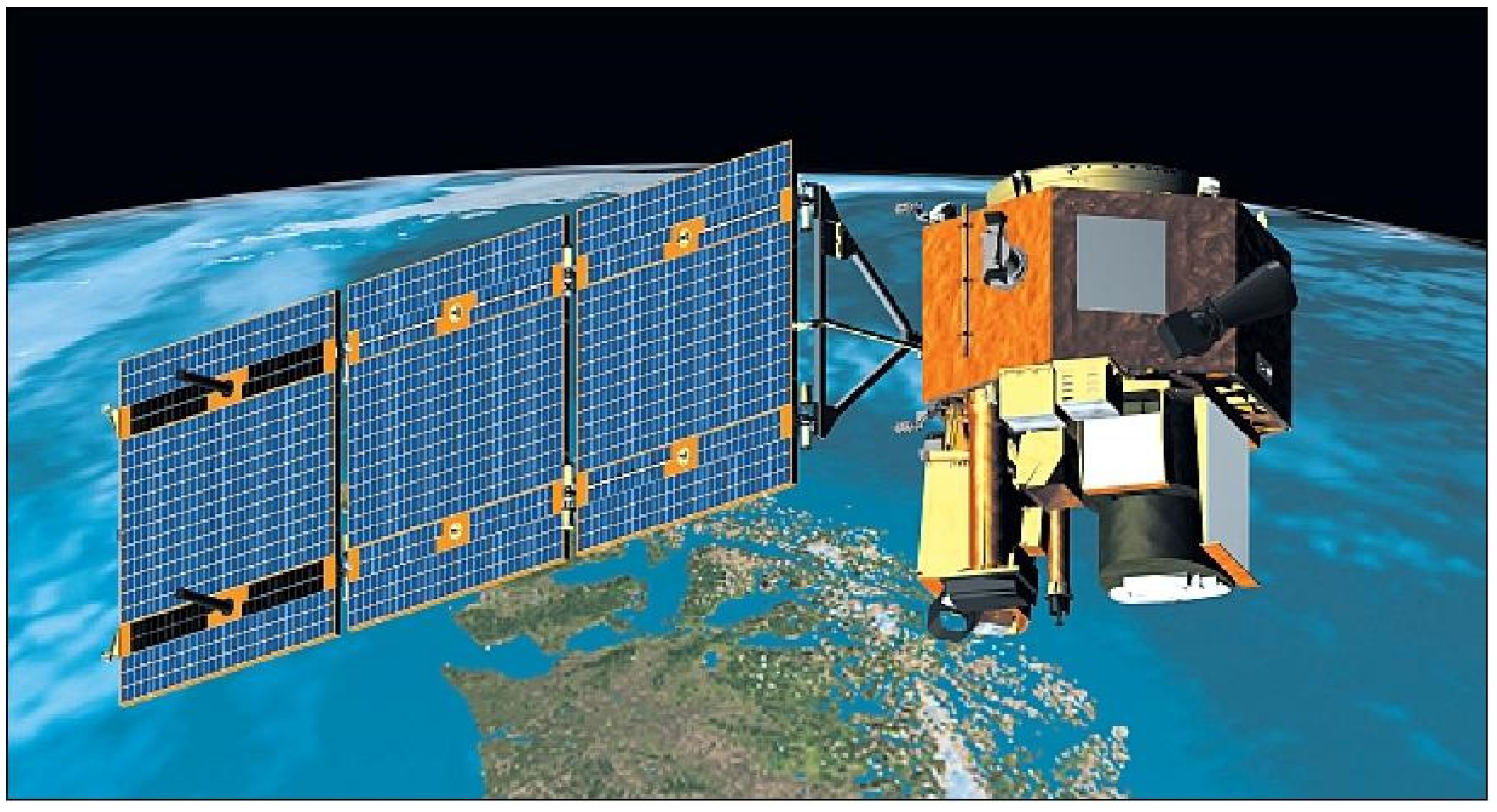
  101. EO-1 (Earth Observing-1). Available online: https://www.eoportal.org/satellite-missions/eo-1#eo-1-earth-observing-1 (accessed on 22 June 2023).
  102. QGIS Software. Available online: https://qgis.org/en/site/ (accessed on 24 June 2023).
  103. Urfa Haber. Available online: https://www.medyaurfa.com/gundem/harran-ovasi-gap-ile-ihya-oldu-h81516.html (accessed on 26 June 2023).
  104. Çimtay, Y.; İlk, H.G. A novel bilinear unmixing approach for reconsideration of subpixel classification of land cover. Comput. Electron. Agric. 2018, 152, 126–140. [Google Scholar] [CrossRef]
  105. Wang, L.; Wei, Y. Revised normalized difference nitrogen index (NDNI) for estimating canopy nitrogen concentration in wetlands. Optik 2016, 127, 7676–7688. [Google Scholar] [CrossRef]
  106. Rouse, J.W.; Haas, R.H.; Schell, J.A.; Deering, D.W. Monitoring Vegetation Systems in the Great Plains with ERTS; Third ERTS Symposium; NASA: Washington, DC, USA, 1973; pp. 309–317.
  107. Gitelson, A.A.; Merzlyak, M.N. Remote Sensing of Chlorophyll Concentration in Higher Plant Leaves. Adv. Space Res. 1998, 22, 689–692. [Google Scholar] [CrossRef]
  108. Huete, A.; Didan, K.; Miura, T.; Rodriguez, E.P.; Gao, X.; Ferreira, L.G. Overview of the Radiometric and Biophysical Performance of the MODIS Vegetation Indices. Remote Sens. Environ. 2002, 83, 195–213. [Google Scholar] [CrossRef]
  109. Sripada, R.P. Determining In-Season Nitrogen Requirements for Corn Using Aerial Color-Infrared Photography. Ph.D. Dissertation, North Carolina State University, Raleigh, NC, USA, 2005. [Google Scholar]
  110. Haboudane, D.; Miller, J.R.; Pattey, E.; Zarco-Tejada, P.J.; Strachan, I.B. Hyperspectral Vegetation Indices and Novel Algorithms for Predicting Green LAI of Crop Canopies: Modeling and Validation in the Context of Precision Agriculture. Remote Sens. Environ. 2004, 90, 337–352. [Google Scholar] [CrossRef]
  111. Vogelmann, J.; Rock, B.; Moss, D. Red Edge Spectral Measurements from Sugar Maple Leaves. Int. J. Remote Sens. 1993, 14, 1563–1575. [Google Scholar] [CrossRef]
  112. Serrano, L.; Penuelas, J.; Ustin, S. Remote Sensing of Nitrogen and Lignin in Mediterranean Vegetation from AVIRIS Data: Decomposing Biochemical from Structural Signals. Remote Sens. Environ. 2002, 81, 355–364. [Google Scholar] [CrossRef]
  113. Deep Learning Toolbox. Available online: https://www.mathworks.com/products/deep-learning.html (accessed on 28 June 2023).
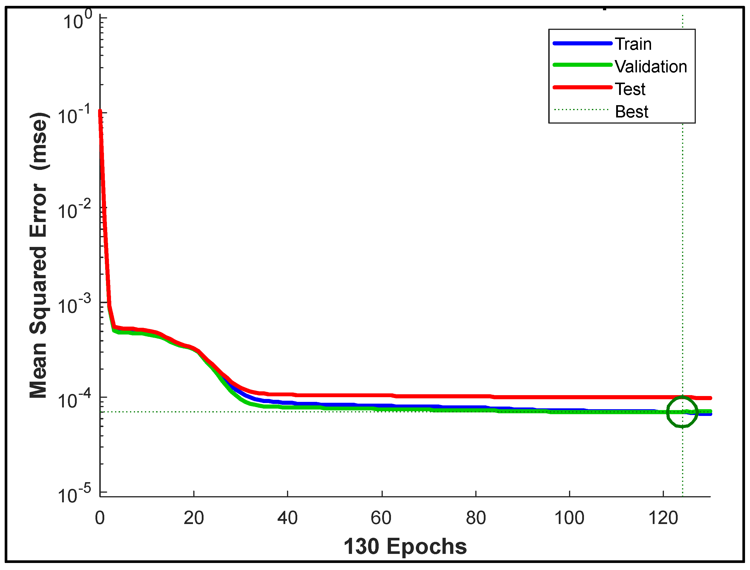
  114. Hagan, M.T.; Menhaj, M.B. Training feedforward networks with the Marquardt algorithm. IEEE Trans. Neural Netw. 1994, 5, 989–993. [Google Scholar] [CrossRef] [PubMed]
  115. Wang, F.-Y. Control 5.0: From Newton to Merton in popper’s cybersocial-physical spaces. IEEE/CAA J. Autom. Sin. 2016, 3, 233–234. [Google Scholar]
Figure 1. EO-1 Satellite View [101].
Remotesensing 15 03898 g001
Figure 2. Google Earth view of Harran (top) and Earth Explorer view of Hyperion (color image) (bottom).
Remotesensing 15 03898 g002
Figure 3. Hyperion data. RGB Image of Harran Region.
Remotesensing 15 03898 g003
Figure 4. Harran plain. Drone camera image (top). Ground image from a cotton field (bottom) [103].
Remotesensing 15 03898 g004
Figure 5. Hyperion image and NDVI Map for Harran. (a) Hyperion color image (b) NDVI Map.
Remotesensing 15 03898 g005
Figure 6. Feed forward deep neural network (proposed).
Remotesensing 15 03898 g006
Figure 7. Regression plots for training, validation, test and all data.
Remotesensing 15 03898 g007
Figure 8. Loss (MSE) for training, validation, test and all data.
Remotesensing 15 03898 g008
Figure 9. Two-deep layer with 25 neurons on Normalized Data.
Remotesensing 15 03898 g009
Figure 10. Two-deep layer with 25 neurons on unnormalized data.
Remotesensing 15 03898 g010
Figure 11. Four-deep layer with 25 neurons on unnormalized data.
Remotesensing 15 03898 g011
Figure 12. Difference image between actual NDNI and estimated NDNI with proposed network.
Remotesensing 15 03898 g012
Table 1. Hyperion sensor parameters.
ParametersHyperion Sensor Details
Spectral range400–2500 nm
Spatial resolution30 m
Radiometric resolution12 bits
Swath width7.5 km
Spectral resolution10 nm
Spectral coverageContinuous
Number of rows, columns, bands3271, 871, 220
Table 2. Number of pixels falling in specific intervals of NDVI values.
NDVI < 00 ≤ NDVI < 0.250.25 ≤ NDVI < 0.50.5 ≤ NDVI < 0.750.75 ≤ NDVI < 1
447,396193,177214,010269,86049
Table 3. Vegetation indices, bands or wavelengths and equations.
IndexBands and/or
Wavelengths
Equation for Estimation
NDVI [106] N I R , R E D N I R     R e d N I R   +   R e d
GNDVI [107] N I R , G r e e n N I R     G r e e n N I R   +   G r e e n
EVI [108] N I R , G r e e n , B l u e 2.5 N I R     R e d N I R   +   6     R e d     7.5     B l u e   +   1
GOSAVI [109] N I R , G r e e n N I R     G r e e n N I R   +   G r e e n   +   0.16
GSAVI [109] N I R , G r e e n 1.5 N I R     G r e e n N I R   +   G r e e n   +   0.5
MCARI2 [110] ρ 800 , ρ 670 , ρ 550 1.5     [ 2.5 ρ 800     ρ 670     1.3 ( ρ 800     ρ 670 ) ] ( 2     ρ 800   +   1 ) 2     6     ρ 800     5     ρ 670     0.5
VREI2 [111] ρ 734 , ρ 747 , ρ 726 , ρ 715 ρ 734     ρ 747 ρ 715   +   ρ 726
NDNI [112] ρ 1510 , ρ 1680 log 1 ρ 1510     log ( 1 ρ 1680 ) log 1 ρ 1510   +   log 1 ρ 1680
Table 4. Regression equations between output and target.
DataEquation for Estimation
Training O u t p u t = 0.87 T a r g e t + 0.0066
Validation O u t p u t = 0.89 T a r g e t + 0.0059
Test O u t p u t = 0.83 T a r g e t + 0.0089
All O u t p u t = 0.87 T a r g e t + 0.0069
Table 5. Benchmark of the proposed method with various regression models.
MethodRegression Score (R2)
Linear Regression−0.29
SVM Regression0.15
Gradient-boosted decision trees (GBDT)0.37
Random Forest Regressor0.46
Stochastic Gradient Descent (SGD)0.35
PLSRegression0.36
Proposed0.91
Table 6. Regression scores obtained by training various neural networks.
Number of Deep LayersNumber of NeuronsRegression Scores
(Train-Validation-Test-All)
2100.93-0.90-0.85-0.91
3100.93-0.92-0.91-0.92
4100.93-0.91-0.92-0.93
5100.93-0.93-0.90-0.93
2150.92-0.92-0.88-0.91
3150.93-0.91-0.90-0.92
4150.95-0.89-0.93-0.94
5150.94-0.94-0.87-0.93
2200.93-0.92-0.91-0.92
3200.93-0.88-0.91-0.92
4200.95-0.92-0.89-0.94
5200.91-0.92-0.90-0.91
2250.91-0.91-0.92-0.91
3250.94-0.90-0.92-0.93
4250.94-0.93-0.91-0.93
5250.92-0.88-0.89-0.91
Disclaimer/Publisher’s Note: The statements, opinions and data contained in all publications are solely those of the individual author(s) and contributor(s) and not of MDPI and/or the editor(s). MDPI and/or the editor(s) disclaim responsibility for any injury to people or property resulting from any ideas, methods, instructions or products referred to in the content.

