

Anticipating the Collapse of Urban Infrastructure: A Methodology Based on Earth Observation and MT-InSAR

Abstract
:1. Introduction
2. Methodology
2.1. Obtaining the LOS Map and Generation of Interferograms
2.2. Extraction of Persistent Scatterers to Monitor Land Deformation
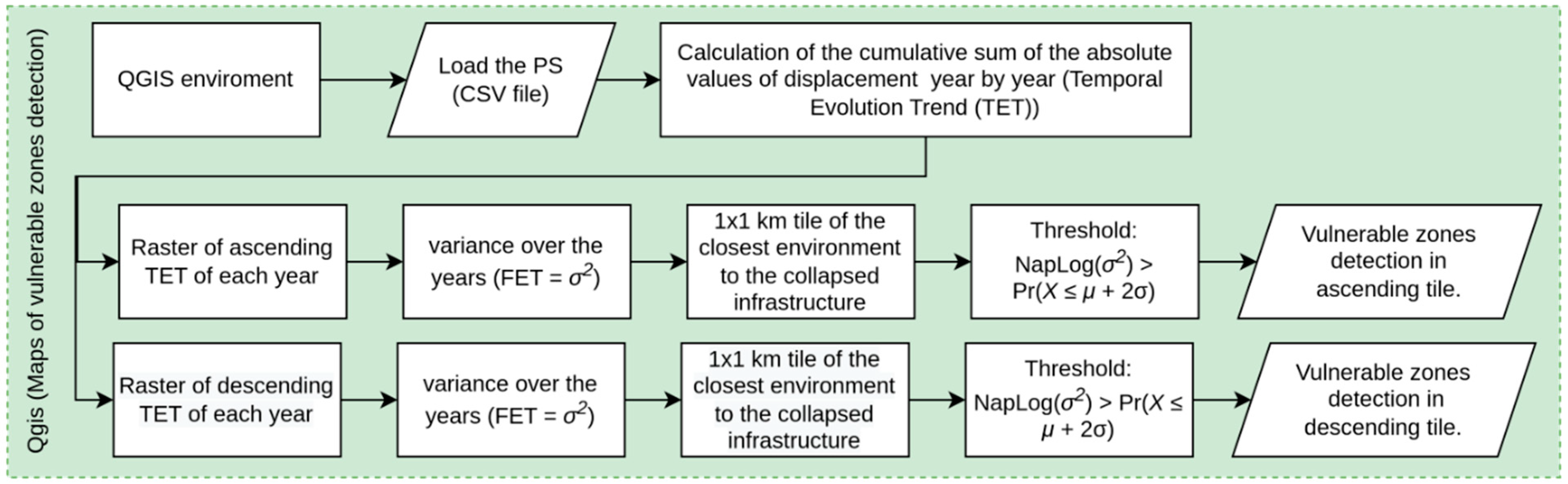
2.3. PS Geospatial Analysis
- σ2 is the variance obtained from the MT-InSAR results of each pixel over the years of the analysis, that is, the FET.
- xi is the absolute displacement of year i (TET).
- μ is the mean of all absolute values of the annual displacement.
- N is the number of years of the total analysis.
3. Experiment and Data Processing
Study Area and Data
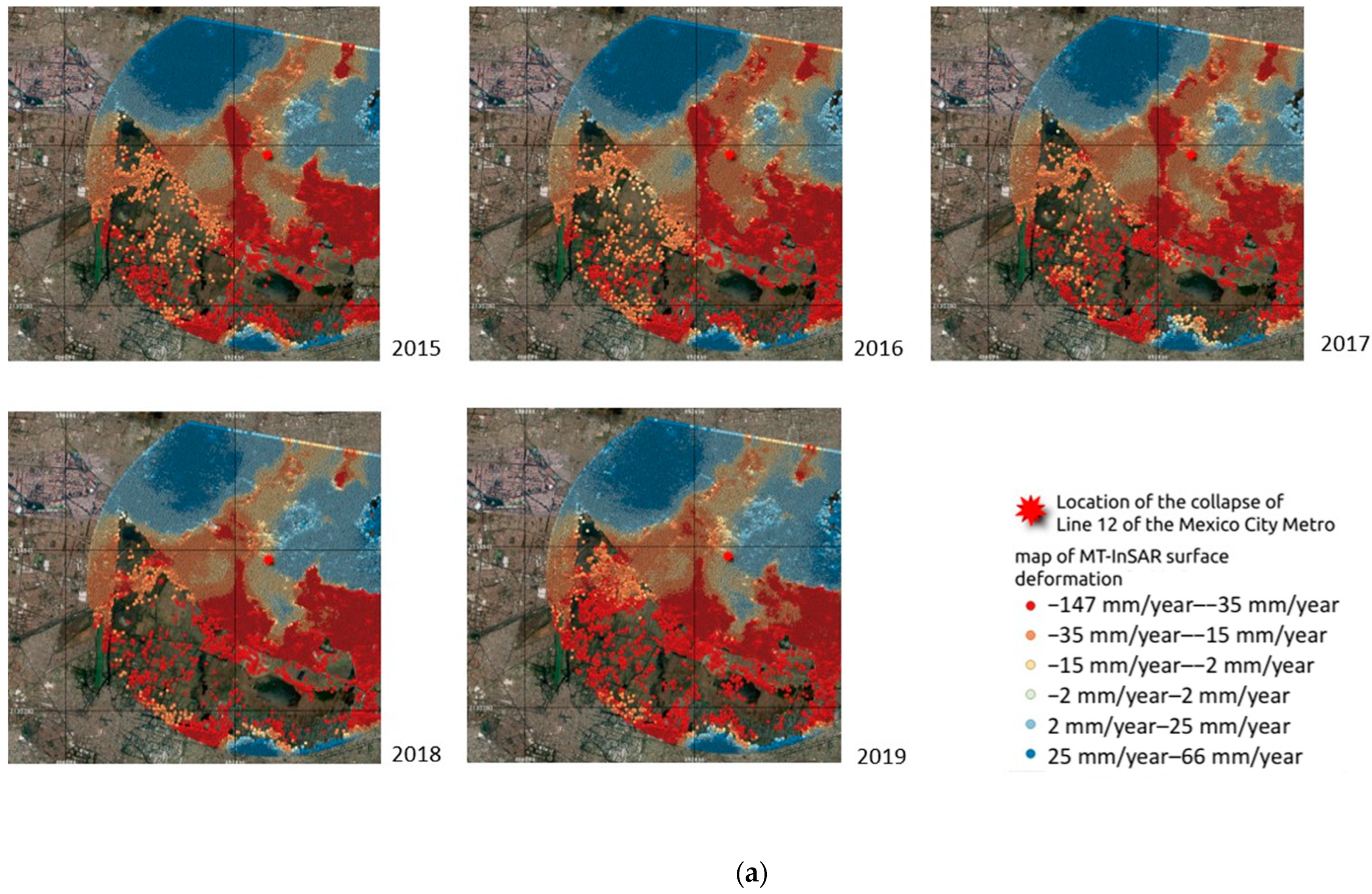
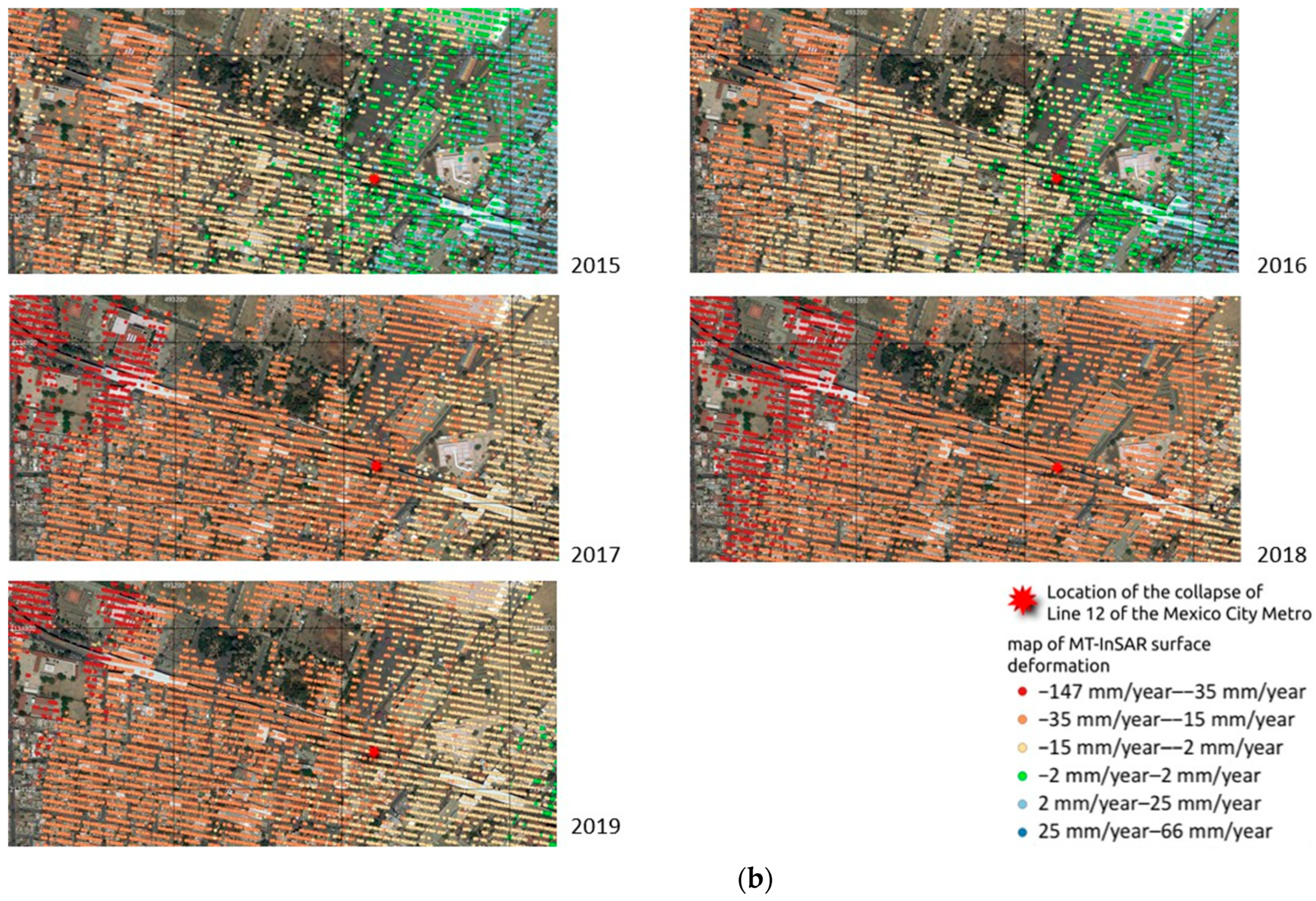
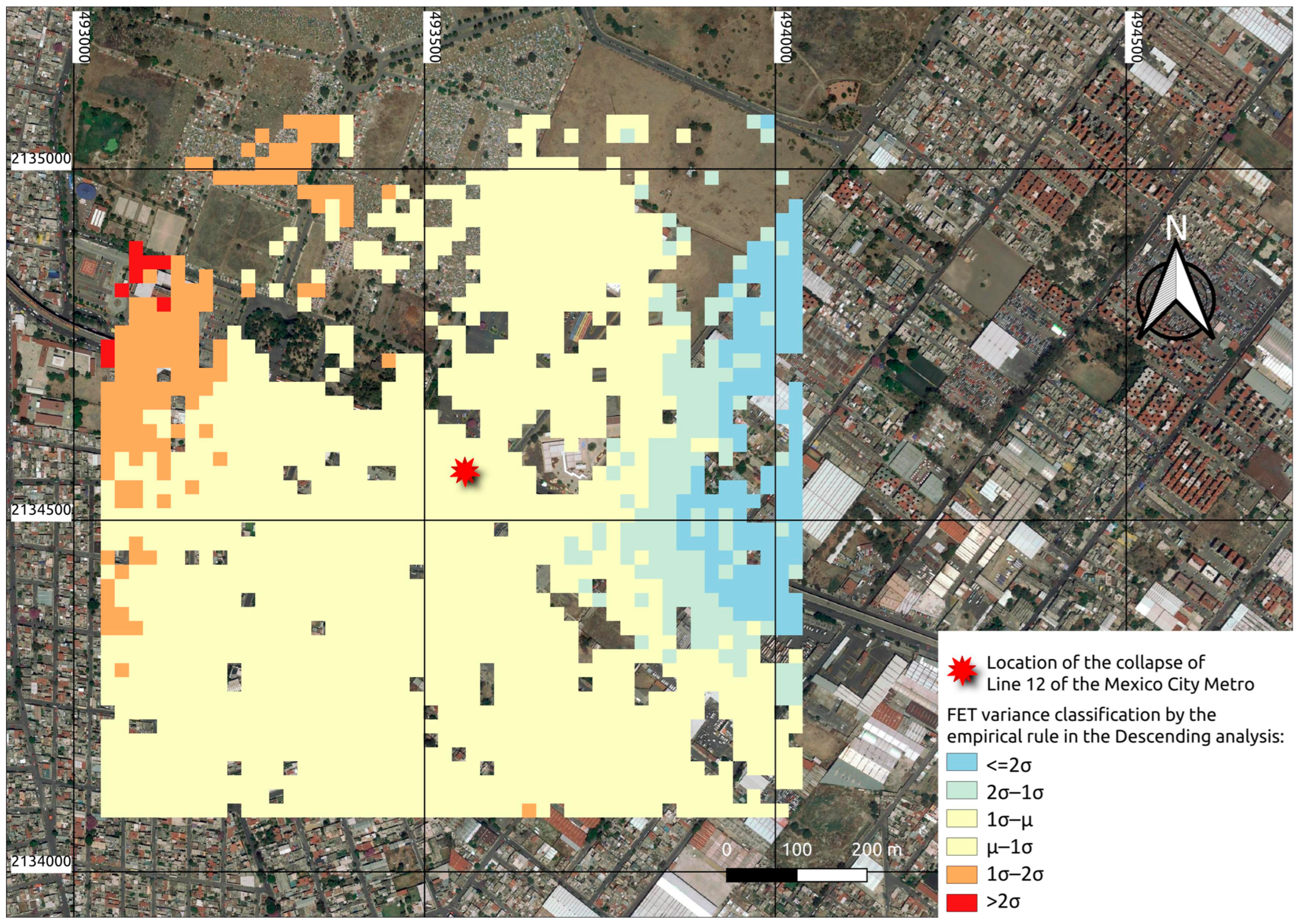
- Infrastructure located in areas of continuous subsidence. Mexico City has experienced multiple earthquakes and is located on top of a lagoon, which makes the area unstable. The specific infrastructure that was analyzed consists of the accident that occurred on 3 May 2021, on Line 12 of the Mexico City Metro. This accident may have been caused by the placement and welding of the bolts that connect the girders of the steel viaduct with the concrete slab [31].
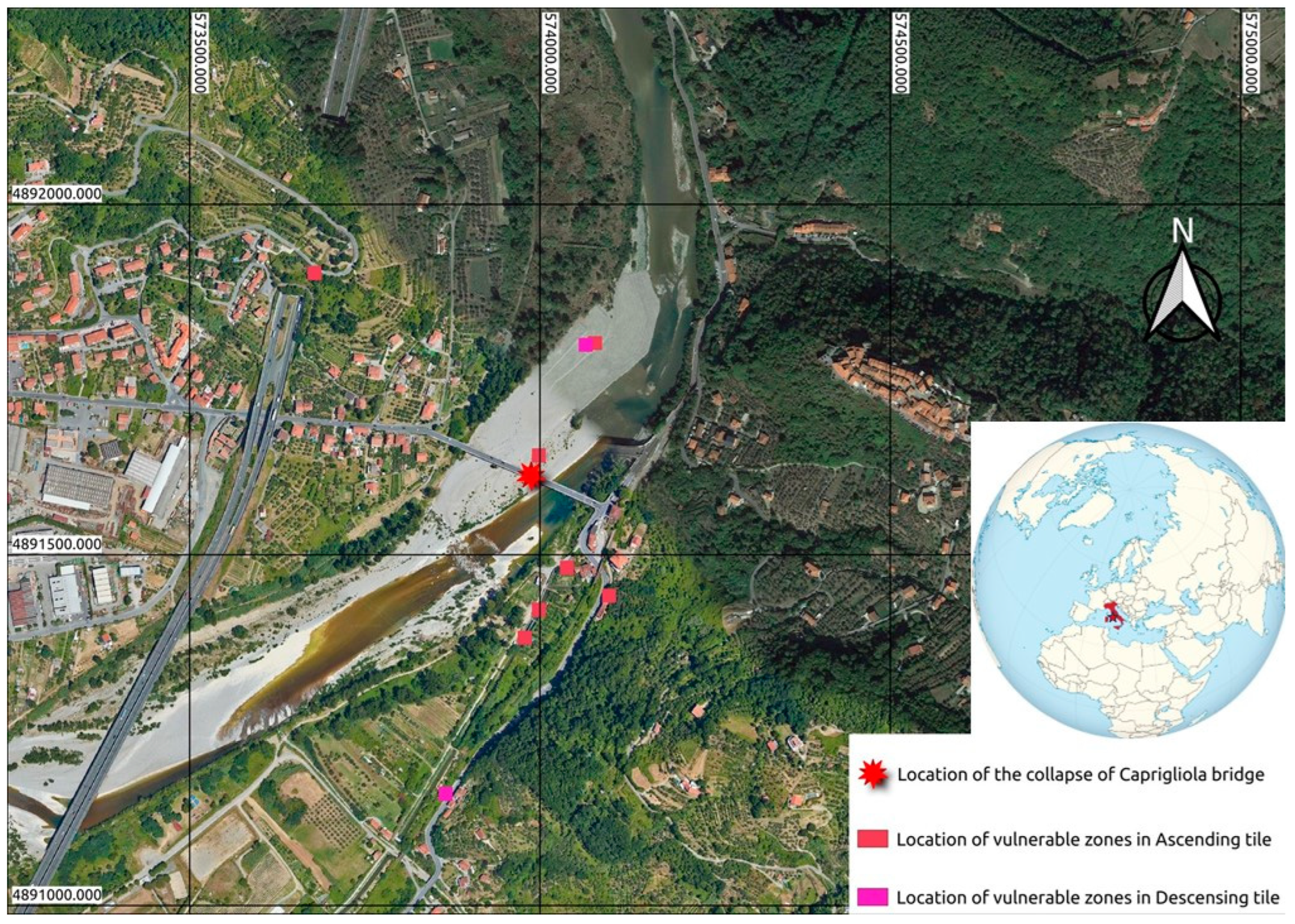
- Infrastructure in semi-urban environments surrounded by vegetation, where two case studies were considered. The first infrastructure analyzed is the Caprigliola bridge (Italy), which collapsed over the Magra river on 8 April 2020. The causes of the collapse are still to be determined [32]. The second infrastructure analyzed consists of a building that partially collapsed in Peñíscola (Spain), on 25 August 2021 [33].
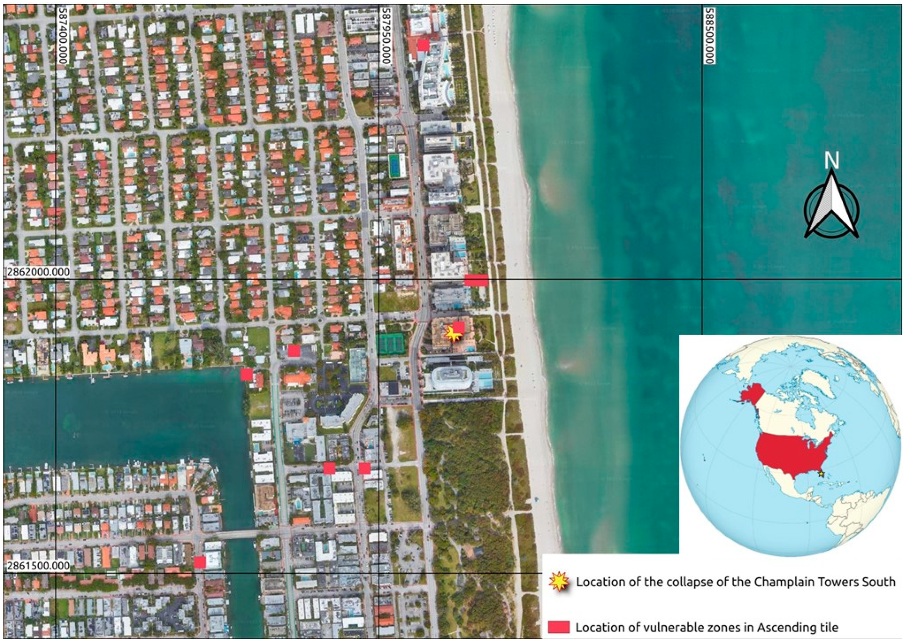
- Infrastructure in coastal environments. On 24 June 2021, the Champlain Towers South, a 12-story condominium located in the beachfront suburb of Surfside, Miami (United States), partially collapsed. The degradation of the reinforced concrete structural support, attributed to water penetration and corrosion of the reinforcing steel, is being studied as the focus of the causes for the collapse. This evidence was identified in 2018 and worsened by April 2021 [34]. Other contributing factors being considered include land subsidence, insufficient reinforcing steel, and corruption during construction [35,36]. The Surfside collapse is considered the third largest building failure in the history of the United States [37].
4. Results and Analysis
5. Discussion
6. Conclusions
Author Contributions
Funding
Conflicts of Interest
References
- Enrico, A.; Grosso, D.; Del Grosso, A.E. Structural Health Monitoring: Research and Practice. Structural Health Monitoring, Lifecycle and BIM View Project Parametric Design, Form Finding and Optimisation of Shell, Gridshell and Spatial Structures View Project Structural Health Monitoring: Research and Practice. 2013. Available online: https://www.researchgate.net/publication/261119109 (accessed on 13 February 2023).
- Moreu, F.; Li, X.; Li, S.; Zhang, D. Technical specifications of structural health monitoring for highway bridges: New chinese structural health monitoring code. Front. Built Environ. 2018, 4, 10. [Google Scholar] [CrossRef] [Green Version]
- Kaneko, S.; Toyota, T. Long-term urbanization and land subsidence in Asian megacities: An indicators system approach. In Groundwater and Subsurface Environments: Human Impacts in Asian Coastal Cities; Springer: Berlin/Heidelberg, Germany, 2011; pp. 249–270. [Google Scholar] [CrossRef]
- Wang, H.M.; Wang, Y.; Jiao, X.; Qian, G.R. Risk management of land subsidence in Shanghai. Desalination Water Treat. 2014, 52, 1122–1129. [Google Scholar] [CrossRef]
- Solarski, M.; Machowski, R.; Rzetala, M.; Rzetala, M.A. Hypsometric changes in urban areas resulting from multiple years of mining activity. Sci. Rep. 2022, 12, 2982. [Google Scholar] [CrossRef]
- Xue, F.; Lv, X.; Dou, F.; Yun, Y. A Review of Time-Series Interferometric SAR Techniques: A Tutorial for Surface Deformation Analysis. Institute of Electrical and Electronics Engineers Inc. IEEE Geosci. Remote Sens. Mag. 2020, 8, 22–42. [Google Scholar] [CrossRef]
- Nádudvari, Á. Using radar interferometry and SBAS technique to detect surface subsidence relating to coal mining in Upper Silesia from 1993–2000 and 2003–2010. Environ. Socio-Econ. Stud. 2016, 4, 24–34. [Google Scholar] [CrossRef] [Green Version]
- Przylucka, M.; Herrera, G.; Graniczny, M.; Colombo, D.; Béjar-Pizarro, M. Combination of Conventional and Advanced DInSAR to Monitor Very Fast Mining Subsidence with TerraSAR-X Data: Bytom City (Poland). Remote Sens. 2015, 7, 5300–5328. [Google Scholar] [CrossRef] [Green Version]
- MacChiarulo, V.; Milillo, P.; Blenkinsopp, C.; Reale, C.; Giardina, G. Multi-temporal InSAR for transport infrastructure monitoring: Recent trends and challenges. Proc. Inst. Civ. Eng. Bridge Eng. 2021, 176, 92–117. [Google Scholar] [CrossRef]
- Malik, K.; Kumar, D.; Perissin, D.; Pradhan, B. Estimation of ground subsidence of New Delhi, India using PS-InSAR technique and Multi-sensor Radar data. Adv. Space Res. 2022, 69, 1863–1882. [Google Scholar] [CrossRef]
- Chang, L.; Dollevoet, R.P.B.J.; Hanssen, R.F. Monitoring Line-Infrastructure with Multisensor SAR Interferometry: Products and Performance Assessment Metrics. IEEE J. Sel. Top. Appl. Earth Obs. Remote Sens. 2018, 11, 1593–1605. [Google Scholar] [CrossRef] [Green Version]
- Free and Open Source Software (FOSS). Available online: https://en.unesco.org/freeandopensourcesoftware (accessed on 3 January 2022).
- Ferretti, A.; Prati, C.; Rocca, F. Nonlinear subsidence rate estimation using permanent scatterers in differential SAR interferometry. IEEE Trans. Geosci. Remote Sens. 2000, 38, 2202–2212. [Google Scholar] [CrossRef] [Green Version]
- Blasco, J.D.; Foumelis, M.; Stewart, C.; Hooper, A. Measuring Urban Subsidence in the Rome Metropolitan Area (Italy) with Sentinel-1 SNAP-StaMPS Persistent Scatterer Interferometry. Remote Sens. 2019, 11, 129. [Google Scholar] [CrossRef] [Green Version]
- Bakon, M.; Perissin, D.; Lazecky, M.; Papco, J. Infrastructure Non-linear Deformation Monitoring via Satellite Radar Interferometry. Procedia Technol. 2014, 16, 294–300. [Google Scholar] [CrossRef] [Green Version]
- Chang, L.; Dollevoet, R.P.B.J.; Hanssen, R.F. Nationwide Railway Monitoring Using Satellite SAR Interferometry. IEEE J. Sel. Top. Appl. Earth Obs. Remote Sens. 2017, 10, 596–604. [Google Scholar] [CrossRef]
- Sousa, J.J.; Bastos, L. Multi-temporal SAR interferometry reveals acceleration of bridge sinking before collapse. Nat. Hazards Earth Syst. Sci. 2013, 13, 659–667. [Google Scholar] [CrossRef]
- Bischoff, C.A.; Ferretti, A.; Novali, F.; Uttini, A.; Giannico, C.; Meloni, F. Nationwide deformation monitoring with SqueeSAR® using Sentinel-1 data. Proc. Int. Assoc. Hydrol. Sci. 2020, 382, 31–37. [Google Scholar] [CrossRef] [Green Version]
- Raspini, F.; Bianchini, S.; Ciampalini, A.; Del Soldato, M.; Montalti, R.; Solari, L.; Tofani, V.; Casagli, N. Persistent Scatterers continuous streaming for landslide monitoring and mapping: The case of the Tuscany region (Italy). Landslides 2019, 16, 2033–2044. [Google Scholar] [CrossRef] [Green Version]
- Raspini, F.; Bianchini, S.; Ciampalini, A.; Del Soldato, M.; Solari, L.; Novali, F.; Del Conte, S.; Rucci, A.; Ferretti, A.; Casagli, N. Continuous, semi-automatic monitoring of ground deformation using Sentinel-1 satellites. Sci. Rep. 2018, 8, 7253. [Google Scholar] [CrossRef] [PubMed] [Green Version]
- Del Soldato, M.; Solari, L.; Raspini, F.; Bianchini, S.; Ciampalini, A.; Montalti, R.; Ferretti, A.; Pellegrineschi, V.; Casagli, N. Monitoring Ground Instabilities Using SAR Satellite Data: A Practical Approach. ISPRS Int. J. Geo-Inf. 2019, 8, 307. [Google Scholar] [CrossRef] [Green Version]
- Zhu, M.; Wan, X.; Fei, B.; Qiao, Z.; Ge, C.; Minati, F.; Vecchioli, F.; Li, J.; Costantini, M. Detection of Building and Infrastructure Instabilities by Automatic Spatiotemporal Analysis of Satellite SAR Interferometry Measurements. Remote Sens. 2018, 10, 1816. [Google Scholar] [CrossRef] [Green Version]
- Barra, A.; Solari, L.; Béjar-Pizarro, M.; Monserrat, O.; Bianchini, S.; Herrera, G.; Crosetto, M.; Sarro, R.; González-Alonso, E.; Mateos, R.M.; et al. A Methodology to Detect and Update Active Deformation Areas Based on Sentinel-1 SAR Images. Remote Sens. 2017, 9, 1002. [Google Scholar] [CrossRef] [Green Version]
- Luo, S.; Feng, G.; Xiong, Z.; Wang, H.; Zhao, Y.; Li, K.; Deng, K.; Wang, Y. An Improved Method for Automatic Identification and Assessment of Potential Geohazards Based on MT-InSAR Measurements. Remote Sens. 2021, 13, 3490. [Google Scholar] [CrossRef]
- Tomás, R.; Pagán, J.I.; Navarro, J.A.; Cano, M.; Pastor, J.L.; Riquelme, A.; Cuevas-González, M.; Crosetto, M.; Barra, A.; Monserrat, O.; et al. Semi-Automatic Identification and Pre-Screening of Geological–Geotechnical Deformational Processes Using Persistent Scatterer Interferometry Datasets. Remote Sens. 2019, 11, 1675. [Google Scholar] [CrossRef] [Green Version]
- Bianchini, S.; Solari, L.; Casagli, N.; Tomás, R.; Löw, F.; Thenkabail, P.S. A GIS-Based Procedure for Landslide Intensity Evaluation and Specific risk Analysis Supported by Persistent Scatterers Interferometry (PSI). Remote Sens. 2017, 9, 1093. [Google Scholar] [CrossRef] [Green Version]
- SNAP—STEP. Available online: http://step.esa.int/main/toolboxes/snap/ (accessed on 4 January 2021).
- Blasco, J.M.D.; Foumelis, M. Automated SNAP Sentinel-1 DInSAR Processing for StaMPS PSI with Open Source Tools. In Proceedings of the International Geoscience and Remote Sensing Symposium 2018 (IGARSS 2018), Valencia, Spain, 22–27 July 2018. [Google Scholar] [CrossRef]
- GitHub-dbekaert/StaMPS: Stanford Method for Persistent Scatterers. Available online: https://github.com/dbekaert/stamps (accessed on 16 January 2023).
- StaMPS/2-4_StaMPS-steps.md Master Matthias/gis-Blog GitLab. Available online: https://gitlab.com/Rexthor/gis-blog/-/blob/master/StaMPS/2-4_StaMPS-steps.md (accessed on 10 February 2021).
- Por Qué Colapsó la Línea 12 del Metro de Ciudad de México—The New York Times. Available online: https://www.nytimes.com/es/interactive/2021/06/12/espanol/america-latina/metro-ciudad-de-mexico.html (accessed on 3 January 2022).
- È Crollato un Ponte su una Strada Provinciale tra Toscana e Liguria—Il Post. Available online: https://www.ilpost.it/2020/04/08/crollo-ponte-liguria-toscana-aulla-bolano/ (accessed on 3 January 2022).
- Semana Clave para Conocer las Causas del Derrumbe en Peñíscola que Costó la Vida a dos Personas|Radio Valencia|Cadena SER. Available online: https://cadenaser.com/emisora/2021/09/25/radio_valencia/1632567036_278947.html (accessed on 3 January 2022).
- Why Did This Florida Condo Building Collapse? Experts Explain. The New York Times. Available online: https://www.nytimes.com/2021/06/27/us/miami-building-investigation-clues.html (accessed on 3 January 2022).
- Corruption in North Miami Beach Could Be Factor in Surfside Building Collapse: 7 Things to Know. Available online: https://moguldom.com/362247/corruption-in-north-miami-beach-could-be-factor-in-surfside-building-collapse-7-things-to-know/ (accessed on 3 January 2022).
- Surfside Condo Built in Era Tainted by Corruption|Fred Grimm—South Florida Sun Sentinel—South Florida Sun-Sentinel. Available online: https://web.archive.org/web/20210714183615/https://www.sun-sentinel.com/opinion/commentary/fl-op-com-grimm-south-florida-building-inspectors-corruption-20210702-6u6kamfs4vcefatc6iqbidns6y-story.html (accessed on 3 January 2022).
- Surfside Condo Collapse Is Third Largest Building Failure in Country’s History—CBS Miami. Available online: https://miami.cbslocal.com/2021/06/29/surfside-condo-collapse-third-largest-building-failure-us-history/ (accessed on 3 January 2022).
- European Ground Motion Service—Copernicus Land Monitoring Service. Available online: https://land.copernicus.eu/pan-european/european-ground-motion-service (accessed on 20 January 2023).


| Parameter | Default | Used |
|---|---|---|
| max_topo_err | 20 | 10 |
| filter_grid_size | 50 | 40 |
| clap_win | 32 | 16 |
| scla_deramp | ‘n’ | ‘y’ |
| percent_rand | 20 | 1 |
| unwrap_grid_size | 200 | 50 |
| unwrap_time_win | 730 | 180 |
| scn_time_win | 365 | 180 |
| scn_wavelength | 100 | 50 |
| unwrap_gold_n_win | 32 | 16 |
| Pixel Classification | Threshold |
|---|---|
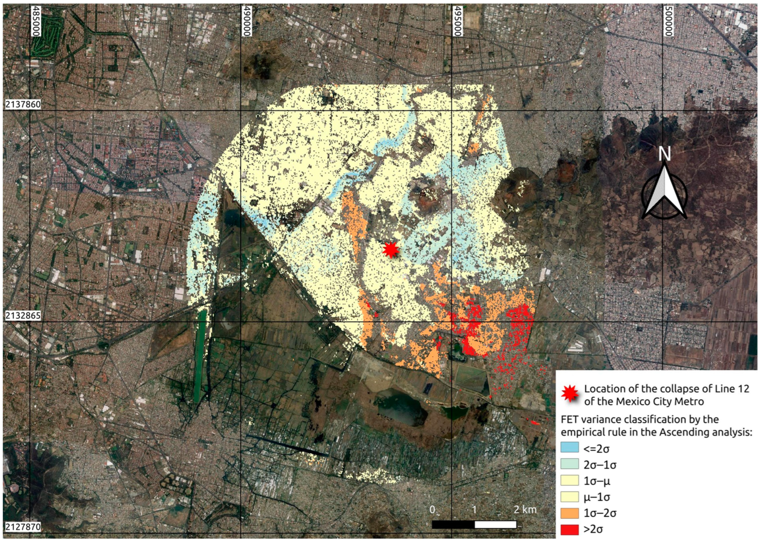
| Stable areas | NapLog(σ2) < Pr(μ − 2σ ≤ X ≤ μ + 2σ) |
| Vulnerable areas | NapLog(σ2) < Pr(X ≤ μ + 2σ) |
| Case Study | Ascending 2 | Descending 3 |
|---|---|---|
| Line 12 of the Mexico City Metro | 23 March 2015 to 2 May 2021 | 20 March 2015 to 29 April 2021 |
| Caprigliola bridge | 2 August 2015 to 7 April 2020 | 12 October 2015 to 6 April 2020 |
| Building in the Font Nova urbanization (Peñiscola) | 24 March 2015 to 12 May 2017 and 4 October 2018 to 25 August 2021 | 30 March 2015 to 13 March 2017 and 4 October 2018 to 25 August 2021 |
| Miami | 9 October 2016 to 21 June 2021 | No data |
| Case Study | Number of Alert Pixels in Tile | Minimum Distance between the Actual Structure Collapse and the Nearest Collapse Risk Alert Pixel |
|---|---|---|
| Line 12 of the Mexico City Metro | 9 | ≅540 m (concurs with one of the girders supporting the overpass carrying Line 12 of the Mexico City Metro near the Tezonco station) |
| Caprigliola bridge | 9 | ≅20 m (in the streambed where the bridge collapsed) |
| Building in the Font Nova urbanization (Peñiscola) | 30 | ≅65 m (coincides geographically with the environment of the collapsed building) |
| Miami | 9 | ≅0.50 m (exact geographical overlay on the collapsed building) |
Disclaimer/Publisher’s Note: The statements, opinions and data contained in all publications are solely those of the individual author(s) and contributor(s) and not of MDPI and/or the editor(s). MDPI and/or the editor(s) disclaim responsibility for any injury to people or property resulting from any ideas, methods, instructions or products referred to in the content. |
© 2023 by the authors. Licensee MDPI, Basel, Switzerland. This article is an open access article distributed under the terms and conditions of the Creative Commons Attribution (CC BY) license (https://creativecommons.org/licenses/by/4.0/).
Share and Cite
Rodríguez-Antuñano, I.; Martínez-Sánchez, J.; Cabaleiro, M.; Riveiro, B. Anticipating the Collapse of Urban Infrastructure: A Methodology Based on Earth Observation and MT-InSAR. Remote Sens. 2023, 15, 3867. https://doi.org/10.3390/rs15153867
Rodríguez-Antuñano I, Martínez-Sánchez J, Cabaleiro M, Riveiro B. Anticipating the Collapse of Urban Infrastructure: A Methodology Based on Earth Observation and MT-InSAR. Remote Sensing. 2023; 15(15):3867. https://doi.org/10.3390/rs15153867
Chicago/Turabian StyleRodríguez-Antuñano, Ignacio, Joaquín Martínez-Sánchez, Manuel Cabaleiro, and Belén Riveiro. 2023. "Anticipating the Collapse of Urban Infrastructure: A Methodology Based on Earth Observation and MT-InSAR" Remote Sensing 15, no. 15: 3867. https://doi.org/10.3390/rs15153867