Article

Monitoring Spartina alterniflora Expansion Mode and Dieback Using Multisource High-Resolution Imagery in Yancheng Coastal Wetland, China

1
College of Horticulture and Plant Protection, Henan University of Science and Technology, Luoyang 471023, China
2
College of Biology and the Environment, Co-Innovation Center for Sustainable Forestry in Southern China, Nanjing Forestry University, Nanjing 210037, China
*
Author to whom correspondence should be addressed.
Remote Sens. 2023, 15(15), 3853; https://doi.org/10.3390/rs15153853
Submission received: 19 May 2023 / Revised: 25 July 2023 / Accepted: 1 August 2023 / Published: 3 August 2023
(This article belongs to the Special Issue Remote Sensing for Wetland Restoration)

Abstract

:
Spartina alterniflora (smooth cordgrass), China’s most common invasive species, has posed significant challenges to native plant communities and coastal environments. Monitoring the invasion and dieback process of S. alterniflora by multisource high-resolution imagery is necessary to manage the invasion of the species. Current spatial analyses, however, are insufficient. As a result, we first extracted S. alterniflora by integrating multisource high-resolution images through the multiscale object-oriented classification method, then identified the expansion patterns of S. alterniflora on the seaward side by the landscape expansion index, and conformed the main drivers of S. alterniflora dieback on the landward side in the Jiangsu Dafeng Milu National Nature Reserve. The findings revealed that the area of S. alterniflora decreased in size from 1511.26 ha in 2010 to 910.25 ha in 2020. S. alterniflora continues to grow to the sea and along the tidal creek on the seaward side, with a total increase of 159.13 ha. External isolation expansion patterns accounted for 65.16% of the total expansion patches, with marginal expansion patches accounting for 24.22% and tidal creek-leading expansion patches accounting for 10.62%. While the landward side showed a declining trend, the total area decreased by 852.36 ha, with an annual average change rate of 8.67%. S. alterniflora dieback was negatively related to the number of tidal creeks and positively related to the number of wild Elaphures davidianus and the length of artificial ditches. Our findings provide a scientific foundation for the ecological control of S. alterniflora. Its presence in coastal wetlands inspires evidence-based protection and management strategies to protect the coastal wetland ecosystem.

Graphical Abstract

1. Introduction

Spartina alterniflora (S. alterniflora), as the most widespread invasive species, has been widely introduced to many countries and regions for reducing erosion, reclaiming land, improving soil, purifying water quality, and stabilizing the coast [1,2,3]. However, due to its strong dispersal and reproductive abilities, S. alterniflora has occupied the majority of the tidal flat wetlands along China’s coast from Liaoning to the Leizhou Peninsula for nearly 40 years [4,5,6]. As a result, the Ministry of Environmental Protection of China designated it as one of the sixteen most dangerous invasive plants in China in 2003 [2]. Currently, numerous research studies have demonstrated that S. alterniflora negatively affects native vegetation communities and coastal environments by displacing native plant species [7,8], interfering with the hydrodynamic deposition process of coastal wetlands [9,10], changing the characteristics of the local environment, and even reducing biodiversity [1,11]. Therefore, the correct scientific evaluation of S. alterniflora invasion dynamics and an examination of internal driving mechanisms are crucial for the scientific management and control of S. alterniflora.
Nowadays, we are incapable of accurately distinguishing invasive plants in the ecotone and producing a detailed map in a small area with high precision. Furthermore, S. alterniflora and native plants have similar spectral characteristics and have been affected by tidal inundation for a long time [10,12]. A large number of studies have been conducted to monitor and map the spatial distribution of S. alterniflora at various spatial and temporal scales including supervised classification works based on pixel and object-based image analysis (OBIA) [3,4,13,14]. Landsat imagery, with its medium spatial resolution and nearly 40-year time span, has been the most widely used data for describing dynamic changes in invasive vegetation [3,15,16,17]. Liu et al. investigates the expansion of S. alterniflora by using Landsat and OBIA methods along the Chinese coast from 1990 to 2015 [15]. Yan et al. used GEE and object-based hierarchical random forest classification methods to extract the spatial distribution of S. alterniflora in Jiangsu Province and analyzed its expansion and dieback [3]. However, it is especially ineffective at distinguishing small patches in the early stages of expansion [1,10,12]. Some researchers believe that high-resolution imagery is required to provide more accurate and detailed data [18,19]. Chen et al. used multisource high-resolution satellite images and deep-learning super-resolution methods to accurately depict small patches of early onset S. alterniflora [20]. Dai et al. extracted the size, number, and area of early patches of S. alterniflora based on unmanned aerial vehicle (UAV) images, which confirmed the feasibility of using an UAV to observe the self-organization process of saltmarsh vegetation [21]. Therefore, high-resolution imagery can provide more accurate and detailed data for monitoring S. alterniflora. The landscape pattern and its dynamic research has always been an important scientific problem in landscape ecology [22]. High-resolution images are more suitable for the timely detection and recognition of the invasion pattern of S. alterniflora [23]. Most of the previous methods are based on static landscape indices, with little attention paid to landscape spatial processes [1,24]. To overcome the limitations of the landscape pattern index and enable it to express dynamic information of landscape patterns, some scholars have proposed the landscape dynamic index [25,26]. Wu et al. proposed a new landscape expansion index (LEI) to identify the pattern of landscape spatial expansion, and explore the relationship between landscape expansion and the original landscape pattern [26]. Wang et al. identified three expansion patterns of S. alterniflora: marginal expansion, external isolated expansion and tidal creek-leading expansion through LEI and the patch fractal dimension, which will be helpful for understanding the invasive mechanism of S. alterniflora [26]. However, previous studies focused on monitoring the dynamic change of area of S. alterniflora in a long time period.
Saltmarsh dieback, also known as brown marsh, occurs when the leaves of the saltmarsh vegetation begin to turn yellow brown and eventually die. As the area of the saltmarsh vegetation decreases significantly, the saltmarsh or vegetation degrades and becomes a mudflat [3,27]. Tidal creeks are tidal channels that develop on tidal flats. The spatiotemporal distribution and geometric structural characteristics of tidal creeks control the flow, sedimentation rate, nutrients, and vegetation community structure of tidal flats [28,29]. The tidal-creek network structure represents the tidal flats’ hydrological connectivity. The more tidal creeks, the better the hydrological connectivity. Tidal-creek hydrological connectivity can have a significant impact on the energy and ecosystem stability of tidal flats. The greater the tidal-creek network’s hydrological connectivity, the more conducive to the circulation and exchange of nutrient and energy information it is, thereby facilitating the colonization and diffusion of organisms, further maintaining the stability of the habitat’s biological population and improving the resistance and resilience of the community to external disturbances [29,30]. Elaphures davidianus (E. davidianus) is a large herbivorous animal. It only eats the tender leaves of S. alterniflora, and collective feeding inhibits the growth of S. alterniflora. Meanwhile, the behavior of E. davidianus trampling and lying down restricted the growth of S. alterniflora [31,32]. For the mature S. alterniflora with a height of about 2 m, E. davidianus tend to choose this place as the hidden area. Finally, the feces of E. davidianus have a chemical inhibition on S. alterniflora. S. alterniflora is generally yellow and not growing well in the lodging ground of E. davidianus, where there are more E. davidianus feces [33]. Yan et al. found that under the effects of hydro-ecological engineering and the number of E. davidianus, the area of S. alterniflora significantly decreased from 2011 to 2020 [3]. The dynamic changes of S. alterniflora include expansion and dieback. However, there have been few studies on S. alterniflora dieback and its main driving factors in China’s coastal areas.
We developed a classification method to monitor the S. alterniflora expansion mode and dieback in Dafeng Milu National Nature Reserve (DMNNR) using multisource high-resolution imagery. Currently, there is little research on the expansion mode of S. alterniflora and the primary driving forces of S. alterniflora dieback on the Chinese coast. As a result, the DMNNR on the Yellow Sea coast of Jiangsu, China, was chosen as a case study area that has been affected by S. alterniflora invasion and dieback from 2010 to 2020. Our specific goals are as follows: (1) extract S. alterniflora by combining multisource high-resolution images and object-based classification; (2) to examine the expansion dynamics and identify the expansion mode of S. alterniflora on the seaward side; and (3) to investigate the dieback dynamics and identify the primary driving factors of S. alterniflora dieback on the landward side.

2. Materials and Methods
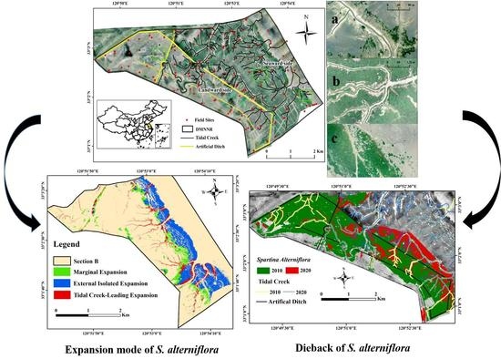
2.1. Study Area

Jiangsu Dafeng Milu National Nature Reserve (DMNNR, 32°56′N~33°36′N, 120°42′E~120°51′E) is located on the southeast of Dafeng, Yancheng City, Jiangsu. DMNNR was founded in 1986, and designated as a national nature reserve in 1997. It was designated as a Wetland of International Importance in 2002, and it is now the world’s largest wild E. davidianus breeding ground. The third core area of the DMNNR and its coastal mudflat were used as a study area in this paper (Figure 1), which is a coastal tidal-flat wetland formed by silting up over the last 30 years, with little human activity and an area of 25 km2. The salt content of the soil and water is more than 3% all the year [34], making it ideal for the growth of S. alterniflora. Meanwhile, due to a lack of natural enemies, S. alterniflora have spread rapidly in the coastal tidal flats and occupied a large area of bare flats, becoming the study area’s single dominant species. As a result, biodiversity has declined sharply, and wetland function is also deteriorating [3,6].
In order to effectively control the spread of S. alterniflora, the reserve has built a total of 2.5 km of small dikes and 10 km of freshwater artificial ditches for wild E. davidianus to create a suitable habitat for wildlife and birds from 2010 to 2018 (Figure 1). At the moment, significant progress has been made in the control of S. alterniflora in the DMNNR. Furthermore, the reserve has been conducting wild-release trials of E. davidianus in batches since 1998, bringing the total number of E. davidianus in the third core area from 156 in 2010 to 1820 in 2020 [3,24]. Additionally, the annual area of S. alterniflora decreased significantly since 2018, which was attributable to it being foraged and trampled [6]. Here, to quantify the long-term expansion and dieback of S. alterniflora, the study area was divided into two parts, the landward side and seaward side, based on the impact of E. davidianus, with the artificial ditch used as the boundary. The landward side was mainly affected by wild E. davidianus and was used to analyze the dieback of S. alterniflora. The seaward side was not affected by E. davidianus and was mainly used to study the seaward expansion of S. alterniflora.

2.2. Preprocessing and DATA acquisition

Land-cover data from 2010 to 2020 were acquired from cloud-free high-resolution images, including WorldView-2(WV-2), GaoFen-2(GF-2), P1eiades-2, Dabai II, and fixed-wing UAV images (Table 1). This study made use of WV-2 imagery collected on 9 November 2011. The WV-2 sensor has four multispectral bands: blue, green, red and near-infrared (NIR). The multispectral spatial resolution of WV-2 imagery was 1.8 m and the panchromatic resolution was 0.5 m. The GF-2 image is a Chinese-developed optical remote sensing satellite, with a panchromatic band (1 m spatial resolution) and four multispectral bands (4 m spatial resolution). On 2 December 2012, the French company Astrium launched the P1eiades-2 satellite. The P1eiades-2 images include a panchromatic band with a spatial resolution of 0.5 m and four multispectral bands with a spatial resolution of 1.8 m. The optical images from the P1eiades-2 satellite used in this study were acquired on 13 September 2013 and 23 December 2018. Figure S1 shows multisource high-resolution images. Most satellite images corresponding to the low tide are taken for this study to eliminate the influence of the tide. The 2013 imagery collected at middle tide, which submerged part of the mudflat, but did not submerge saltmarsh vegetation, affected the detectability of the area of S. alterniflora. The image processing system ENVI (Environment for Visualizing Images, Research Systems, Inc, Broomfield, CO, USA) was used for all preprocessing and analysis of the four images above, including radiometric calibration, atmospheric correction, geometric correction, and image fusion. Finally, 50 ground-control points (Figure S2) measured by the Trimble R8 Global Navigation Satellite System (GNSS) RTK were used for geographic registration (the root mean squared error of geometric rectification was less than 0.5 pixels).
Two regular UAV flights were conducted at a height of 500 m during the low-tide window on 13 August 2020 (UAV platform: Dabai II; wingspan 2.7 m; RGB camera: NIKON D800 (35 mm); flight speed: 30 m/s) to acquire multitemporal RGB imagery over the study area. The vertical and horizontal positioning accuracy of the GNSS is 7–8 cm and 8–10 cm, respectively. The forward overlap heading and side overlap are set to 60% and 40%, respectively, to avoid the impact of lighting conditions on images. Finally, over 1000 camera images were gathered. Meanwhile, the Trimble R8 GNSS RTK used ground-control points (50 points distributed across the study area) for image georeferencing (Figure S2). Agisoft PhotoScan software Version 1.2.5 (Agisoft, St. Petersburg, Russia) generated the high-resolution RGB orthophoto from original RGB images [35].
During the 2020 growing season, a large-scale field survey sampling was carried out. A measurement interval was set every 500 m, and a total of 140 sampling points were collected including 99 S. alterniflora sampling points, 34 mudflat sampling points and 7 other vegetation-type sampling points. Each sampling point’s geographic coordinates were recorded using the Trimble Geo7X differential global positioning system (Figure 1). Due to the difficulty of field investigation in coastal wetlands and the limited number of field samples, this study fully considers the differences in spectral and spatial distribution between Spartina and non-Spartina, and then selected the objects with uniform distribution as samples to supplement the field validation sample points based on the characteristics of different samples obtained from the field survey and multisource high-resolution remote-sensing images. Finally, 300 sample points were selected from 2010 to 2020, respectively, with 70% being training samples and 30% being validation samples.

2.3. Methodologies

2.3.1. Methods for Classifying S. alterniflora and Evaluating Accuracy

S. alterniflora extraction is divided into three stages: (1) multiscale optimal segmentation; (2) object-based random forest classification; and (3) accuracy assessment. The flow diagram for obtaining S. alterniflora is depicted in Figure 2.
(1)
Multiscale optimal segmentation
The most important step in object-oriented classification is multiscale segmentation, which combines homogeneous pixels to form a polygon object. Polygon objects have the highest internal homogeneity and the highest heterogeneity with adjacent polygon objects. Multiscale segmentation is a region-merging algorithm that works from the bottom up and is based on minimum heterogeneity [36,37]. In this study, multiscale segmentation is used to find the local optimal scale segmentation parameters using Estimation of Scale Parameter 2 (ESP2). The image is initially segmented into three levels [38]. The initial multiscale segmentation parameters are set to 1, 50, and 100 with step sizes of 1, 3, and 5, respectively. We give more weight to color than shape, thus the color factor was set to 0.8 and the shape factor was set to 0.2; both smoothness and compactness were set to 0.5, and we segmented the image and calculated the rate of change of local variation (ROC-LV). The segmentation scale local variance curve was generated after 100 iterations (Figure 3a). The optimal segmentation scale is obtained when the local variance reaches a maximum. Because several features have multiple optimal scales, Figure 3a shows two relatively large peaks. When the first peak of the local variance curve is reached, the corresponding segmentation scale 50 can be used as a fine scale to distinguish small patches of S. alterniflora and other vegetation types in a small area from the mudflat (Figure 3b). The scale 99 represents the second peak value and is used as a coarser scale for image segmentation to describe a large area of evenly distributed S. alterniflora, water surfaces, and mudflats (Figure 3c). Mudflats and large area S alterniflora are densely distributed, with large patches that can combine homogeneous objects to improve operation speed and classification accuracy.
(2)
Random Forest Classification Based on Objects
To classify the S. alterniflora, an object-oriented method in conjunction with random forest (RF) was used first. The classification feature space is constructed, which includes spectral features, spectral index, shape features, and texture features, as shown in Table 2. Second, the RF classifier is trained and used. RF has been shown in numerous studies to be a high-precision wetland classification method. The number of classification features and the classification tree of each node in the RF are critical to the accuracy of the classification results [39,40]. By default, tree was set to 50 and try to the square root of the total number of input features in this study. A total of 140 training samples were collected for S. alterniflora community, mudflat, water surface and other vegetation. The RF classifier was trained using the training samples’ feature parameters. The trained RF classifier was used to automatically classify various ground objects. Based on Google Earth high-resolution images and field-survey data, the misclassified objects in the automatic classification were visually interpreted and modified. Finally, the spatial distribution of the S. alterniflora community was determined from 2010 to 2020.

2.3.2. Pattern Recognition in S. alterniflora Expansion

Landscape expansion index (LEI) detects pattern and scales of landscape expansion [25,26]. LEI was used in this study to analyze and examine S. alterniflora patch expansion patterns. The LEI equation is as follows:
L E I = A p A 0 A p + A 0
where A0 represents the original area of S. alterniflora patch, and Ap is the expansion area of S. alterniflora patch. When A0 ≠ 0, the LEI is (−1,1), and its expansion mode is marginal expansion, which expands outward from the original patch, and the newly generated patch is adjacent to the previous S. alterniflora patch. When A0 = 0, LEI = 1, indicating that the original area of S. alterniflora patch is zero, its expansion pattern is external isolation expansion mode or tidal-creek-leading expansion mode. The characteristics of external isolation expansion is that seeds of S. alterniflora land on the mudflat and quickly grow into an approximate circle, and then continue to expand outward with the circle at the center. The tidal-creek-leading expansion mode demonstrates that after the seeds of S. alterniflora are planted on both sides of the tidal creek, they expand along both sides of the tidal creek. The patch fractal dimension (PFD) reflects the landscape patch rules and complexity. The greater the complexity of the edges, the greater the PFD; conversely, the simpler the patch boundary, the lower the fragmentation degree [43]. As a result, the PFD can be used to tell the difference between the external isolation patch and the tidal-creek-leading patch. Arcgis 10.5 and Fragstat 4.2 software were used in this study to calculate the LEI and PFD indexes.

2.3.3. Correlation Analysis between Dieback of S. alterniflora and Main Driving Factors

The object-oriented classification method is used to obtain the distribution of the mudflat and water surface based on multisource high-resolution remote-sensing images from 2010 to 2020. The spatial distribution of tidal creeks and artificial ditches is extracted using the visual interpretation method by vectoring the axes of tidal creeks and artificial ditches. Because the tidal creek network takes decades to reach equilibrium, the overall change in the tidal creek in the last ten years was negligible. As a result, we began by manually visualizing the tidal-creek network in 2010. The tidal-creek data for 2013 were obtained by manually supplementing and modifying the tidal-creek data from 2010. As a result, the two periods’ unchanged tidal-creek parts are consistent, and the false changes caused by the inconsistency of the two tidal-creek centers due to visual interpretation are avoided. In 2016, 2018, and 2020, the same method was used to determine the spatial distribution and length changes of tidal creeks and artificial ditches (Figure 4). The number of E. davidanus was obtained from Jiangsu Dafeng Milu National Nature Reserve. Correlation analysis between the dieback of S. alterniflora and the main driving factors was conducted using OriginPro 2021b.

3. Results

3.1. Accuracy Evaluation of S. alterniflora Maps

The number of field samples is limited due to the difficulty of field investigation in coastal wetland. As a result of the 2020 field sampling data, a total of 100 verification points were obtained, including 78 validation points of the S. alterniflora community and 22 validation points of the non-S. alterniflora community (17 mudflat validation points and five other vegetation validation points). We assessed the accuracy of S. alterniflora Maps by the error matrixes, user accuracies (UAs), producer accuracies (PAs), overall accuracies (OAs), and kappa coefficients (Supplementary B). The overall classification accuracy was 0.97, and the Kappa coefficient was 0.86, indicating that the S. alterniflora classification results in 2020 were in good agreement with the actual distribution. Due to a lack of field sampling data in 2018, 2016, 2013, and 2010, we generated 100 sampling points on Google Earth high-resolution images for each year. The results showed that the overall accuracy of the classification results was 0.93, 0.95, 0.93 and 0.95, and the Kappa coefficients were 0.78, 0.85, 0.82 and 0.76 in 2018, 2016, 2013, and 2010, respectively, which proved that the classification accuracy of S. alterniflora from 2010 to 2020 meets the application requirements of this study (Table 3).

3.2. Area and Distribution of S. alterniflora from 2010 to 2020

The S. alterniflora area and the rate of change from 2010 to 2020 are listed in Table 4. S. alterniflora-classification results in the DMNNR are shown in Figure 5. The total area decreased by 601.02 ha, with an annual change rate of 3.98%, from 1511.26 ha in 2010 to 910.25 ha in 2020. In the year 2010, the S. alterniflora in the reserve reached a maximum of 1511.26 ha, accounting for 87% of the total study area. It was distributed in a belt-like pattern along the coast toward the sea. Between 2010 to 2013, the S. alterniflora decreased slightly to 1508.24 ha with S. alterniflora transforming into mudflat in the northwest of the study area. Furthermore, S. alterniflora spread to the sea, primarily occupying mudflats on the seashore. The area of S. alterniflora was basically stable in 2016, decreasing by 0.26 ha. The shift in spatial distribution is consistent with what was observed in 2013. In the year 2018, the S. alterniflora began to significantly decrease, with a total decrease of 162.98 ha and an annual rate of change of 5.40% from 1507.97 ha in 2016 to 1345.0 ha in 2018. On the landward side, the spatial pattern of S. alterniflora began to diminish significantly. In the northwest, there was almost no S. alterniflora. It continued to decline significantly from 2018 to 2020, with a total area reduction of 434.75 ha and a maximum annual change rate of 16.16%. The landward side of the study area has all turned into a beach, while the seaward side of S. alterniflora is slowly expanding toward the sea. As a result, from 2010 to 2020, S. alterniflora demonstrated a process of decreasing on the land side and increasing on the sea side, but the area of expansion was smaller than the area of reduction.

3.3. Expansion mode of S. alterniflora from 2010 to 2020

Figure 6 depicts the spatial expansion of S. alterniflora on the seaward side from 2010 to 2020. S. alterniflora area increased by 159.13 ha, rising from 525.51 ha in 2010 to 684.64 ha in 2020. The spatial distribution of S. alterniflora in the northeast of the study did not extend significantly to the sea (Figure 6b), whereas it did in the southeast (Figure 6c). S. alterniflora not only grows continuously to the sea, but it also grows along the tidal creek (Figure 6a). As a result, it is critical for expansion dynamics to analyze and identify the expansion pattern.
The expansion modes of the S. alterniflora patch included external isolation expansion, tidal-creek-leading expansion, and marginal expansion (Figure 7). Table 5 displays the statistics of the LEI interval distribution. The LEI can be used to identify various expansion patterns. When the LEI value is (−1,1), the S. alterniflora spatial expansion pattern is marginal expansion. When LEI = 1 and PFD < 1.4, the S. alterniflora spatial expansion pattern is external isolation expansion; and when LEI = 1 and PFD ≥ 1.4, the S. alterniflora spatial expansion pattern is tidal-creek-leading expansion.
Between 2010 to 2020, S. alterniflora expanded by 11,706 patches, covering a total area of 279.47 ha. The number of external isolation expansion patches among them was 7628, with an area of 166.88 ha, accounting for 65.16% of the total number of expansion patches, indicating that the S. alterniflora community expanded primarily through external isolation expansion. Only 1243 patches, with an area of 41.32 ha and a proportion of 10.62%, were dominated by the tidal-creek-led expansion mode, which was critical in the development of the tidal-creek system. There are 2835 marginal expansion patches totaling 71.24 ha, accounting for 24.22% of the total. Although the marginal expansion of the S. alterniflora community is a small-scale expansion, it cannot be overlooked.

3.4. Dieback Dynamics of S. alterniflora and Main-Driving-Factors Correlation Analysis

To investigate the main causes of S. alterniflora dieback, Pearson correlation analysis was carried out between the distribution area of S. alterniflora, as well as the number of tidal creeks, the length of artificial ditches, and the number of E. davidianus from 2010 to 2020. On the landward side, the area of S alterniflora had a significant positive correlation with the number of tidal creeks (r= 0.93) at the 0.05 level, indicating that the greater number of tidal creeks, the greater area of S. alterniflora, and vice versa. There was, however, a significant inverse relationship between the area of S. alterniflora and the length of artificial ditches (r= −0.79), and the number of E. davidianus (r = −0.98) at the 0.01 level. It demonstrates that the greater length of the artificial ditch, the greater the number of E. davidianus, and the smaller the area of S. alterniflora, and vice versa (Figure 8).
The size of S. alterniflora on the landward side declined from 985.73 ha in 2010 to 133.36 ha in 2020, a total loss of 852.36 ha (Table 6). There were 90 tidal creeks in 2010, and the network’s hydrological connectivity was relatively high. Meanwhile, no artificial ditches were constructed, and the E. davidianus population was small (Figure 9b). As a result, the conditions were best suited for the growth of S. alterniflora. In 2018, The number of tidal creeks decreased to 18 on the landward side, and the tidal creek network in the study area essentially vanished; so, the area of S. alterniflora decreased to 711.20 ha. The number of tidal ditches and the length of artificial ditches did not change from 2018 to 2020, but the number of E. davidianus increased significantly, with a total decrease of 577.84 ha. As a result, the increase in the number of E. davidianus is the primary cause of the reduction in the area of S. alterniflora (Figure 9c).

4. Discussion

4.1. Multisource High-Resolution Imagery’s Potential and Reliability in Monitoring S. alterniflora Invasion

DMNNR was chosen as a case study in our study to investigate the potential use of multisource high-resolution images for monitoring the S. alterniflora dynamic. The dynamic expansion of S. alterniflora had been reported in a few studies in the DMNNR based on a medium-resolution Landsat image [3,24]. Landsat, with a resolution of 30 m, can only detect a distribution area of S. alterniflora if it is larger than 30 m pixels in size. As a result, classifying Spartina pixels with other mixed pixels is difficult [44,45,46]. We compared our findings to those of Landsat, and discovered that from 2011 to 2013, Landsat images divided the mixed pixels of S. alterniflora and mudflat into S. alterniflora; the classification area of high-resolution images is smaller than the classification area of S. alterniflora in Landsat-image classification results. However, Landsat images from 2016 to 2020 divide the mixed pixels into mudflats (Figure 10a,b), resulting in the area of S. alterniflora being smaller in the Landsat images than in high-resolution classification [3]. In this study, we discovered that high-resolution images have significant advantages in detecting S. alterniflora on a smaller scale. First, the newly expanded S. alterniflora patches are scattered on the tidal flat and are highly fragmented. They are difficult to detect using Landsat and other medium-resolution images [44,45,46], but they can be well identified using high-resolution data (Figure 10c,d). Secondly, S. alterniflora grows along the tidal creek’s banks. S. alterniflora patches are relatively long and narrow, but not particularly large in area, and they can be extracted to further investigate S. alterniflora expansion patterns (Figure 10e,f). Finally, because of E. davidianus foraging on and trampling on the Spartina saltmarsh, there are only scattered small S. alterniflora patches on both sides of the tidal creek. Multiscale segmentation was used to separate S. alterniflora patches into individual small objects (Figure 10g,h). The above analysis shows that high-resolution and object-oriented methods can not only extract large areas of evenly distributed S. alterniflora, but also extract small areas of scattered patches of S. alterniflora in order to achieve the goal of the fine extraction of the S. alterniflora community.

4.2. Expansion Mode of S. alterniflora on the Seaward between 2010 and 2020

On the seaward side, S. alterniflora is expanding to the sea and along the tidal creek (Figure 6). Three expansions mode were identified by LEI and PFD. External isolation expansion accounted for 65.16% of the total expansion patches, which indicated that the speed and area of external isolation expansion are greater than those of marginal expansion and tidal-creek-leading expansion models. In the external isolation expansion mode, the sexual reproduction of S. alterniflora is of great significance to the development of new habitats, that is, they first occupy a new habitat in mudflat with seeds, and then expand into invasion patches by tillering reproduction. The number of patches with external isolation expansion is the largest, and the fragmentation trend is serious, which also indicates that S. alterniflora mainly expands to the sea in recent years [16,47]. There are 2835 marginal expansion patches, which mainly rely on underground rhizomes for tillering reproduction, and the highly developed aerenchyma can provide sufficient oxygen for its roots to facilitate the growth of adjacent S. alterniflora [48]. Only 1243 tidal-creek-leading expansion patches account for 10.62% of the total patches. Despite its small distribution area, the tidal-creek-leading expansion pattern is critical for the development of the tidal-creek system. Seeds and rhizomes drift with the tide to germinate and settle at the edge of the tidal channel, and then rely on tillering reproduction to continuously expand along both sides of the tidal creek [49]. At the same time, the continuous expansion of S. alterniflora will also affect the development of the tidal-flat surface and tidal creek. The invasion of S. alterniflora makes the tidal-flat surface continuously silted up, thus changing the tidal dynamics. The expansion of three modes is dominated by tillering reproduction, which is similar to the creation of a buffer zone outside the existing patches, but the tidal and wind effects will make S. alterniflora seeds settle in the mudflat and generate new patches [25,48,49].

4.3. The Relationship between Spartina Saltmarsh Dieback and Main Driving Factors

Between 2010 and 2020, the S. alterniflora on the landward side declined, with a total loss of 852.36 ha. The geographical distribution of S. alterniflora was found to be positively related to the number of tidal creeks and negatively related to the number of E. davidianus and the length of artificial ditches. Tidal creeks are tidal channels that emerged from tidal flats. They are important channels not only for the input and output of tidal water and sediment, but also for the exchange of material, energy, and information between land and sea [50]. The temporal and spatial distribution and geometric structure of tidal creeks control the flow, sedimentation rate, nutrients, and vegetation community structure of tidal flats [28]. The tidal creeks are mostly found on the estuary’s tidal flats, with a flat shape, and a branch-like network structure. This network structure represents the tidal flats’ unique hydrological connectivity. Tidal-creek hydrological connectivity can have a significant impact on the energy and material flow, biodiversity, and ecosystem stability of tidal flats. The greater the tidal-creek network’s hydrological connectivity, the more conducive it is to the circulation and exchange of nutrient and energy information [29,30]. As a result of the construction of artificial ditches, the hydrological connectivity of tidal creeks was severed (Figure 11), further contributing to the decline of S. alterniflora between 2010 and 2018. Furthermore, the continuous expansion of S. alterniflora continued to block tidal creeks, causing them to expand in another direction. As a result, there is a complex feedback relationship between the development of the tidal creek network and the structure of the vegetation community [51,52]. Between 2018 and 2020, the area of S. alterniflora decreased rapidly, by a total of 577.84 ha. In 2020, S. alterniflora scattered on both sides of the tidal creek on the landward side. However, the number of E. davidianus increased significantly from 905 in 2018 to 1820 in DMNNR (Table 6). E. davidianus foraging on and trampling of the Spartina saltmarsh was the main reason for the decrease in S. alterniflora area (Figure S3).
Although our results showed that for tidal creeks, the number of E. davidianus and the length of artificial ditches are decent predictors for the dynamic changes of S. alterniflora, factors such as temperature, soil nutrients (C, N, P, S), sea-level rise, storm and hurricane, carbon sink/source, erosion and accretion of sediment caused by tides [6,53,54] should also be included in future studies to comprehensively explore the effects of various environmental factors on S. alterniflora and improve the accuracy of monitoring S. alterniflora.

5. Conclusions

In this study, we combined the object-oriented method with visual interpretation to track S. alterniflora invasion in DMNNR from 2010 to 2020 using WorldView-2, Pléiades-2, GaoFen-2, and UAV Dabai II in the last ten years; the reserve’s S. alterniflora area has shrunk by 601.02 ha. Because of the impact of wild E. davidianus and the reduced hydrological connectivity of tidal creeks, on the landward side of the study area, the area of S. alterniflora is constantly being reduced. On the seaward side, S. alterniflora is constantly spreading and, moving toward the sea, primarily occupying mudflats. The expansion mode of S. alterniflora is mainly through external isolation expansion, and with a minor amount of edge expansion and tidal-creek-leading expansion. This is the first quantitative study of the main driving factors of S. alterniflora dieback which identifies the expansion patterns of S. alterniflora. The findings will provide a scientific foundation for government agencies to control the invasion S. alterniflora.

Supplementary Materials

The following supporting information can be downloaded at https://www.mdpi.com/article/10.3390/rs15153853/s1: Figure S1: Multisource high-resolution images; Figure S2: The digital orthophoto map and ground control point; Figure S3: The effect of E. davidianus on the expansion of S. alterniflora. Tables S1–S5: Accuracy assessment with the reference of sample points.

Author Contributions

Conceptualization, Z.L. and D.Y.; methodology, D.Y.; software, D.Y., J.L. and S.X.; validation, D.Y., J.L. and S.X.; formal analysis, D.Y. and Y.W.; investigation, D.Y., J.L. and S.X.; resources, D.Y. and J.L.; data curation, D.Y.; writing—original draft preparation, D.Y.; writing—review and editing, D.Y., J.L. and Y.W.; visualization, D.Y.; supervision, D.Y. and J.L.; funding acquisition, Z.L. All authors have read and agreed to the published version of the manuscript.

Funding

The study of this paper was supported by National Natural Science Foundation of China (project no. 41871097, 41471078); PhD Research Startup Foundation of Henan University of Science and Technology (grant no. 13480078); Natural Science Foundation of Henan province (project no. 232300420170).

Data Availability Statement

All high-resolution images data in this paper have been described clearly in Section 2.2. The other data that support the findings of this study are available from the corresponding author on reasonable request.

Conflicts of Interest

The authors declare no conflict of interest.

References

  1. Liu, M.; Li, H.; Li, L.; Man, W.; Jia, M.; Wang, Z.; Lu, C. Monitoring the Invasion of Spartina alterniflora Using Multi-source High-resolution Imagery in the Zhangjiang Estuary, China. Remote Sens. 2017, 9, 539. [Google Scholar] [CrossRef] [Green Version]
  2. Luan, Z.; Yan, D.; Xue, Y.; Shi, D.; Xu, D.; Liu, B.; Wang, L.; An, Y. Research progress on the ecohydrological mechanisms of Spartina alterniflora invasion in coastal wetlands. J. Agric. Resour. Environ. 2020, 37, 469–476. [Google Scholar] [CrossRef]
  3. Yan, D.; Li, J.; Yao, X.; Luan, Z. Quantifying the Long-Term Expansion and Dieback of Spartina Alterniflora Using Google Earth Engine and Object-Based Hierarchical Random Forest Classification. IEEE J. Sel. Top. Appl. Earth Obs. Remote Sens. 2021, 14, 9781–9793. [Google Scholar] [CrossRef]
  4. Liu, M. Remote Sensing Analysis of Spartina Alterniflora in the Coastal Areas of China during 1990 to 2015. Ph.D. Thesis, Chinese Academy of Sciences (Northeast Institute of Geography and Agroecology), Changchun, China, 2018. [Google Scholar]
  5. Liu, X. Spatial Pattern and Changes of Spartina Alterniflora with Different Invasion Ages in Yancheng Coastal Wetlands. Ph.D. Thesis, Nanjing Normal University, Nanjing, China, 2018. [Google Scholar]
  6. Yan, D.; Li, J.; Yao, X.; Luan, Z. Integrating UAV data for assessing the ecological response of Spartina alterniflora towards inundation and salinity gradients in coastal wetland. Sci. Total Environ. 2022, 814, 152631. [Google Scholar] [CrossRef] [PubMed]
  7. Wan, S.; Qin, P.; Liu, J.; Zhou, H. The positive and negative effects of exotic Spartina alterniflora in China. Ecol. Eng. 2009, 35, 444–452. [Google Scholar] [CrossRef]
  8. Zhou, H.; Liu, J.; Qin, P. Impacts of an alien species (Spartina alterniflora) on the macrobenthos community of Jiangsu coastal inter-tidal ecosystem. Ecol. Eng. 2009, 35, 521–528. [Google Scholar] [CrossRef]
  9. Mao, D.; Liu, M.; Wang, Z.; Li, L.; Man, W.; Jia, M.; Zhang, Y. Rapid Invasion of Spartina Alterniflora in the Coastal Zone of Mainland China: Spatiotemporal Patterns and Human Prevention. Sensors 2019, 19, 2308. [Google Scholar] [CrossRef] [Green Version]
  10. Wang, A.; Chen, J.; Jing, C.; Ye, G.; Wu, J.; Huang, Z.; Zhou, C. Monitoring the Invasion of Spartina alterniflora from 1993 to 2014 with Landsat TM and SPOT 6 Satellite Data in Yueqing Bay, China. PLoS ONE 2015, 10, e0135538. [Google Scholar] [CrossRef] [Green Version]
  11. Grosholz, E.D.; Levin, L.A.; Tyler, A.C.; Neira, C. Changes in Community Structure and Ecosystem Function Following Spartina Alterniflora Invasion of Pacific Estuaries; University of California Press: Oakland, CA, USA, 2009. [Google Scholar]
  12. Zuo, P.; Zhao, S.; Liu, C.A.; Wang, C.; Liang, Y. Distribution of Spartina spp. along China’s coast. Ecol. Eng. 2012, 40, 160–166. [Google Scholar] [CrossRef]
  13. Liu, X.; Liu, H.; Gong, H.; Lin, Z.; Lv, S. Appling the One-Class Classification Method of Maxent to Detect an Invasive Plant Spartina alterniflora with Time-Series Analysis. Remote Sens. 2017, 9, 1120. [Google Scholar] [CrossRef] [Green Version]
  14. Nagendra, H.; Lucas, R.; Honrado, J.P.; Jongman, R.H.G.; Tarantino, C.; Adamo, M.; Mairota, P. Remote sensing for conservation monitoring: Assessing protected areas, habitat extent, habitat condition, species diversity, and threats. Ecol. Indic. 2013, 33, 45–59. [Google Scholar] [CrossRef]
  15. Liu, M.; Mao, D.; Wang, Z.; Li, L.; Man, W.; Jia, M.; Ren, C.; Zhang, Y. Rapid Invasion of Spartina alterniflora in the Coastal Zone of Mainland China: New Observations from Landsat OLI Images. Remote Sens. 2018, 10, 1933. [Google Scholar] [CrossRef] [Green Version]
  16. Wang, J.; Xiao, X.; Qin, Y.; Doughty, R.B.; Dong, J.; Zou, Z. Characterizing the encroachment of juniper forests into sub-humid and semi-arid prairies from 1984 to 2010 using PALSAR and Landsat data. Remote Sens. Environ. 2018, 205, 166–179. [Google Scholar] [CrossRef]
  17. Zhang, X.; Xiao, X.; Wang, X.; Xu, X.; Chen, B.; Wang, J.; Ma, J.; Zhao, B.; Li, B. Quantifying expansion and removal of Spartina alterniflora on Chongming island, China, using time series Landsat images during 1995–2018. Remote Sens. Environ. 2020, 247, 111916. [Google Scholar] [CrossRef]
  18. Fuller, D.O. Remote detection of invasive Melaleuca trees (Melaleuca quinquenervia) in South Florida with multispectral IKONOS imagery. Int. J. Remote Sens. 2006, 26, 1057–1063. [Google Scholar] [CrossRef]
  19. Walsh, S.J.; McCleary, A.L.; Mena, C.F.; Shao, Y.; Tuttle, J.P.; González, A.; Atkinson, R. QuickBird and Hyperion data analysis of an invasive plant species in the Galapagos Islands of Ecuador: Implications for control and land use management. Remote Sens. Environ. 2008, 112, 1927–1941. [Google Scholar] [CrossRef]
  20. Chen, M.; Ke, Y.; Bai, J.; Li, P.; Lyu, M.; Gong, Z.; Zhou, D. Monitoring early stage invasion of exotic Spartina alterniflora using deep-learning super-resolution techniques based on multisource high-resolution satellite imagery: A case study in the Yellow River Delta, China. Int. J. Appl. Earth Obs. Geoinf. 2020, 92, 102180. [Google Scholar] [CrossRef]
  21. Dai, W.; Li, H.; Gong, Z.; Zhou, Z.; Li, Y.; Wang, L.; Zhang, C.; Pei, H. Self-organization of salt marsh patches on mudflats: Field evidence using the UAV technique. Estuar. Coast. Shelf Sci. 2021, 262, 107608. [Google Scholar] [CrossRef]
  22. Gardner, R.H.; Urban, D.L. Neutral models for testing landscape hypotheses. Landsc. Ecol. 2007, 22, 15–29. [Google Scholar] [CrossRef]
  23. Laba, M.; Downs, R.; Smith, S.; Welsh, S.; Neider, C.; White, S.; Richmond, M.; Philpot, W.; Baveye, P. Mapping invasive wetland plants in the Hudson River National Estuarine Research Reserve using quickbird satellite imagery. Remote Sens. Environ. 2008, 112, 286–300. [Google Scholar] [CrossRef]
  24. Yan, D.; Li, J.; Xie, S.; Liu, Y.; Sheng, Y.; Luan, Z. Examining the expansion of Spartina alterniflora in coastal wetlands using an MCE-CA-Markov model. Front. Mar. Sci. 2022, 9, 964172. [Google Scholar] [CrossRef]
  25. Wang, J.; Liu, H.; Li, Y.; Liu, L.; Xie, F. Recognition of spatial expansion patterns of invasive Spartina alterniflora and simulation of the resulting landscape-changes. Acta Ecol. Sin. 2018, 38, 5413–5422. [Google Scholar] [CrossRef]
  26. Wu, P.; Zhou, D.; Gong, H. A new landscape expansion index: Definition and quantification. Acta Ecol. Sin. 2012, 32, 4270–4277. [Google Scholar] [CrossRef] [Green Version]
  27. Ogburn, M.B.; Alber, M. An investigation of salt marsh dieback in Georgia using field transplants. Estuaries Coasts 2006, 29, 54–62. [Google Scholar] [CrossRef]
  28. Eom, J.; Choi, J.-K.; Ryu, J.-H.; Woo, H.J.; Won, J.-S.; Jang, S. Tidal channel distribution in relation to surface sedimentary facies based on remotely sensed data. Geosci. J. 2012, 16, 127–137. [Google Scholar] [CrossRef]
  29. Cui, B.; Cai, Y.; Xie, T.; Ning, Z.; Hua, Y. Ecological effects of wetland hydrological connectivity: Problems ang prospects. J. Beijing Norm. Univ. Nat. Sci. 2016, 52, 738–746. [Google Scholar] [CrossRef]
  30. Luo, M.; Wang, Q.; Qiu, D.; Shi, W.; Ning, Z.; Cai, Y.; Song, Z.; Cui, B. Hydrological connectivity characteristics and ecological effects of a typical tidal channel system in the Yellow River Delta. J. Beijing Norm. Univ., Nat. Sci. 2018, 54, 17–24. [Google Scholar] [CrossRef]
  31. Ding, Y. Preference of Feeding on Spartina alterniflora loisel by Mi- deer in Dafeng National Nature Reserve. Chin. J. Wildl. 2009, 30, 118–120. [Google Scholar] [CrossRef]
  32. Hua, R.; Cui, D.; Liu, J.; Li, S.; Zhao, Y.; Zhang, Y. Winter Diets of Père David’s Deer in Yancheng Wetland, Jiangsu Province, China. Chin. J. Zool. 2020, 55, 1001. [Google Scholar] [CrossRef]
  33. Jia, Y.; Xie, S.; Yuan, H.; Lu, L. Effects of Wild Elk Activities on Some Ecological Indexes of Spartina alterniflora. J. Anhui Agric. Sci. 2022, 50, 63–65. [Google Scholar] [CrossRef]
  34. Yao, X.; Yan, D.; Li, J.; Liu, Y.; Sheng, Y.; Xie, S.; Luan, Z. Spatial Distribution of Soil Organic Carbon and Total Nitrogen in a Ramsar Wetland, Dafeng Milu National Nature Reserve. Water 2022, 14, 197. [Google Scholar] [CrossRef]
  35. Agisoft PhotoScan User Manual: Professional Edition, Version 1.1. Available online: https://docplayer.net/14282795-Agisoft-photoscan-user-manual-professional-edition-version-1-1.html (accessed on 10 May 2022).
  36. Blaschke, T. Object based image analysis for remote sensing. ISPRS J. Photogramm. Remote Sens. 2010, 65, 2–16. [Google Scholar] [CrossRef] [Green Version]
  37. Hossain, M.D.; Chen, D. Segmentation for Object-Based Image Analysis (OBIA): A review of algorithms and challenges from remote sensing perspective. ISPRS J. Photogramm. Remote Sens. 2019, 150, 115–134. [Google Scholar] [CrossRef]
  38. Drǎguţ, L.; Tiede, D.; Levick, S.R. ESP: A tool to estimate scale parameter for multiresolution image segmentation of remotely sensed data. Int. J. Geogr. Inf. Sci. 2010, 24, 859–871. [Google Scholar] [CrossRef] [Green Version]
  39. Breiman, L.; Friedman, J.; Stone, C.J.; Olshen, R.A. Classification and Regresssion Trees; Routledge: New York, NY, USA, 1984. [Google Scholar]
  40. Sheykhmousa, M.; Mahdianpari, M.; Ghanbari, H.; Mohammadimanesh, F.; Ghamisi, P.; Homayouni, S. Support Vector Machine Versus Random Forest for Remote Sensing Image Classification: A Meta-Analysis and Systematic Review. IEEE J. Sel. Top. Appl. Earth Obs. Remote Sens. 2020, 13, 6308–6325. [Google Scholar] [CrossRef]
  41. Gamon, J.A.; Surfus, J.S. Assessing leaf pigment content and activity with a reflectometer. New Phytol. 1999, 143, 105–117. [Google Scholar] [CrossRef]
  42. Gitelson, A.A.; Kaufman, Y.J.; Stark, R.; Rundquist, D. Novel algorithms for remote estimation of vegetation fraction. Remote Sens. Environ. 2002, 80, 76–87. [Google Scholar] [CrossRef] [Green Version]
  43. Li, B.-L. Fractal geometry applications in description and analysis of patch patterns and patch dynamics. Ecol. Model. 2000, 132, 33–50. [Google Scholar] [CrossRef]
  44. Cleve, C.; Kelly, M.; Kearns, F.R.; Moritz, M. Classification of the wildland–urban interface: A comparison of pixel- and object-based classifications using high-resolution aerial photography. Comput. Environ. Urban Syst. 2008, 32, 317–326. [Google Scholar] [CrossRef]
  45. Müllerová, J.; Pergl, J.; Pyšek, P. Remote sensing as a tool for monitoring plant invasions: Testing the effects of data resolution and image classification approach on the detection of a model plant species Heracleum mantegazzianum (giant hogweed). Int. J. Appl. Earth Obs. Geoinf. 2013, 25, 55–65. [Google Scholar] [CrossRef]
  46. Underwood, E.; Ustin, S.; DiPietro, D. Mapping nonnative plants using hyperspectral imagery. Remote Sens. Environ. 2003, 86, 150–161. [Google Scholar] [CrossRef]
  47. Mendelssohn, I.A.; Postek, M.T. Elemental analysis of deposits on the roots of spartina alterniflora loisel. Am. J. Bot. 1982, 69, 904–912. [Google Scholar] [CrossRef]
  48. Hou, M.; Liu, H.; Zhang, H. Effection of tidal creek system on the expansion of the invasive Spartina in the coastal wetland of Yancheng. Acta Ecol. Sin. 2014, 34, 400–409. [Google Scholar] [CrossRef] [Green Version]
  49. Liu, X.; Li, X.; Chen, Y.; Tan, Z.; Li, S.; Ai, B. A new landscape index for quantifying urban expansion using multi-temporal remotely sensed data. Landsc. Ecol. 2010, 25, 671–682. [Google Scholar] [CrossRef]
  50. Vandenbruwaene, W.; Meire, P.; Temmerman, S. Formation and evolution of a tidal channel network within a constructed tidal marsh. Geomorphology 2012, 151–152, 114–125. [Google Scholar] [CrossRef]
  51. Fan, Y.; Zhou, D.; Ke, Y.; Wang, Y.; Wang, Q.; Zhang, L. Quantifying the Correlated Spatial Distributions between Tidal Creeks and Coastal Wetland Vegetation in the Yellow River Estuary. Wetlands 2020, 40, 2701–2711. [Google Scholar] [CrossRef]
  52. Gong, Z.; Mou, K.; Wang, Q.; Qiu, H.; Zhang, C.; Zhou, D. Parameterizing the Yellow River Delta tidal creek morphology using automated extraction from remote sensing images. Sci. Total Environ. 2021, 769, 144572. [Google Scholar] [CrossRef]
  53. Lu, Z.; Xiao, K.; Wang, F.; Wang, Y.; Yu, Q.; Chen, N. Salt marsh invasion reduces recalcitrant organic carbon pool while increases lateral export of dissolved inorganic carbon in a subtropical mangrove wetland. Geoderma 2023, 437, 116573. [Google Scholar] [CrossRef]
  54. Noonan, J.M. Evaluating the Potential for Transfer of Heavy Metals Through Trophic Interactions in Spartina alterniflora and Littorina irrorata. Ph.D. Thesis, College of Charleston, Charleston, SC, USA, 2023. [Google Scholar]
Figure 1. The Dafeng Milu National Nature Reserve is located in Jiangsu, China. The background image is a natural true color of an unmanned aerial vehicle captured on 13 August 2020. (a) Scattered patches of S. alterniflora along the tidal creek; (b) S. alterniflora spread in strips along both sides of the tidal creek; and (c) circle S. alterniflora patches expansion toward the sea in the early stages. Corresponding field photos (A, B, and C, respectively) were taken in August 2020 at the three field sample locations.
Remotesensing 15 03853 g001
Figure 2. Methodology for extracting S. alterniflora from multisource high-resolution imagery.
Remotesensing 15 03853 g002
Figure 3. The rate of change of local variation (ROC-LV) changes as the segmentation scale increases (a); segmentation effects with a fine scale of 50 (b); segmentation effects with a coarser scale of 99 (c).
Remotesensing 15 03853 g003
Figure 4. Extraction results of tidal creek and artificial ditches in the reserve from 2010 to 2020.
Remotesensing 15 03853 g004
Figure 5. Spatial distribution of land cover from 2010 to 2020 in the DMNNR.
Remotesensing 15 03853 g005
Figure 6. (ac) Spatial expansion dynamics of S. alterniflora on seaward side from 2010 to 2020.
Remotesensing 15 03853 g006
Figure 7. Spatial expansion patterns of S. alterniflora in seaward side from 2010 to 2020.
Remotesensing 15 03853 g007
Figure 8. Person correlation between driving factors and Spartina saltmarsh in landward side. Note: Red indicates positive correlations, blue indicates negative correlations, and the degree of concentration of ellipse indicates the strength of the correlation.
Remotesensing 15 03853 g008
Figure 9. Spatial distribution of S. alterniflora, tidal creek, and artificial ditch on the landward side from 2010 to 2020 (a); spatial distribution of S. alterniflora, tidal creek and artificial ditch in 2010 (b); in 2020 (c).
Remotesensing 15 03853 g009
Figure 10. Classification results of S. alterniflora by Landsat images (a,b); by high-resolution imagery(ch).
Remotesensing 15 03853 g010
Figure 11. The hydrological connectivity of S. alterniflora (red ovals) was cut off by artificial ditch in 2020 (a,b); and was not cut off by artificial ditch in 2010 (c,d).
Remotesensing 15 03853 g011
Table 1. Multisource high-resolution image characteristics.
DateSatellite SensorBandResolution (m)Tide Level
9 November 2010WorldView-230.5Low
13 September 2013Pléiades 230.5Middle
27 July 2016GaoFen-241Low
23 December 2018Pléiades 230.5Low
13 August 2020UAV Dabai II30.1Low
Table 2. Feature list of the image objects used for random forest classifier.
Feature TypeDefinition or Description
Spectral featureMean value of all band; Brightness;
Standard deviation of all band
Spectral indexGreen-red ratio index (GRRI) = G r e e n R e d [41];
Normalized green-red difference index (NGRDI) =   G r e e n R e d G r e e n + R e d   [42]
Shape featureArea; Length; Shape index; Density; Compactness Length–width ratio
Texture featureGray-level co-occurrence matrix (GLCM); Homogeneity; GLCM Mean; GLCM Entropy; GLCM Contrast; GLCM Standard deviation; GLCM Correlation
OtherNeighbor distance; Object location
Table 3. Summary of land-cover classification accuracies from 2010 to 2020.
YearSourceClassPAUAOAKappa Coefficient
2010WorldView-2Spartina0.960.980.950.76
Non-Spartina0.880.82
2013Pléiades-2Spartina0.930.970.930.82
Non-Spartina0.920.82
2016GaoFen-2Spartina0.960.970.950.85
Non-Spartina0.900.86
2018Pléiades-2Spartina0.950.960.930.78
Non-Spartina0.840.80
2020UAV Dabai IISpartina0.960.970.970.86
Non-Spartina0.910.87
Table 4. The change of area for S. alterniflora from 2010 to 2020.
YearArea (ha)StageChange of Area (ha)Annual Change Rate (%)
20101511.262010–2013−3.02−0.07
20131508.242013–2016−0.26−0.006
20161507.972016–2018−162.98−5.40
20181344.992018–2020−434.75−16.16
2020910.252010–2020−601.02−3.98
Table 5. Distribution statistic of LEI on different intervals.
Expansion PatternLEI Interval
Distribution
Number of
Patches
Proportion of
Total Number/%
Area/ha
External Isolated Expansion LEI = 1 and PFD < 1.4762865.16%166.88
Tidal-Creek-Leading ExpansionLEI = 1 and PFD ≥ 1.4124310.62%41.32
Marginal Expansion LEI (−1,1)283524.22%71.27
Table 6. Changes of the area of S. alterniflora, the number of tidal creeks, the length of artificial ditches and the number of E. davidianus from 2010 to 2020.
YearArea (ha)The Number of Tidal CreekThe Number of E. davidianusThe Length of the Artificial Ditch (km)
2010985.72901560
2013905.50742152.31
2016840.51603257.01
2018711.201890517.41
2020133.3618182017.41
Disclaimer/Publisher’s Note: The statements, opinions and data contained in all publications are solely those of the individual author(s) and contributor(s) and not of MDPI and/or the editor(s). MDPI and/or the editor(s) disclaim responsibility for any injury to people or property resulting from any ideas, methods, instructions or products referred to in the content.

