Comparison of Data Fusion Methods in Fusing Satellite Products and Model Simulations for Estimating Soil Moisture on Semi-Arid Grasslands

Abstract

In arid and semi-arid areas, soil moisture (SM) plays a crucial role in land-atmosphere interactions, hydrological processes, and ecosystem sustainability. SM data at large scales are critical for related climatic, hydrological, and ecohydrological research. Data fusion based on satellite products and model simulations is an important way to obtain SM data at large scales; however, little has been reported on the comparison of the data fusion methods in different categories. Here, we compared the performance of two widely used data fusion methods, the Ensemble Kalman Filter (EnKF) and the Back-Propagation Artificial Neural Network (BPANN), in the degraded grassland site (DGS) and the alpine grassland site (AGS). The SM data from the Community Land Model 5.0 (CLM5.0) and the Soil Moisture Active and Passive (SMAP) were fused and validated against the observations of the Cosmic-Ray Neutron Sensor (CRNS) to avoid the impacts of scale-mismatch. Results show that compared with the original data sets at both sites, the RMSE of the fused data by BPANN (FD-BPANN) and EnKF (FD-EnKF) had improved by more than 50% and 31%, respectively. Overall, the FD-BPANN performs better than the FD-EnKF because the BPANN method assigned higher weights to input data with better performance and the EnKF method is affected by the strong variabilities of both the fused CLM5.0 and SMAP data and the CRNS data. However, in terms of the percentile range, the FD-BPANN showed the worst performance, with overestimations in the low SM range of 25th percentile (<Q25), because the BPANN method tends to be trapped in a local minimum. The BPANN method performed better in humid areas, then followed by semi-humid areas, and finally arid and semi-arid areas. Moreover, compared with the previous studies in arid and semi-arid areas, the BPANN method in this study performed better.

1. Introduction

Soil moisture (SM) controls water, energy, and carbon cycles, particularly in arid and semi-arid areas [1,2]. Long-term SM data in arid and semi-arid areas are critical to climatical, hydrometeorological, and ecohydrological research [3,4,5,6,7,8].

Currently, three main approaches are used to obtain SM data: in situ measurements [9], satellite products [10], and model simulations [11,12]. In situ measurements are the most accurate method to directly observe SM, but it is expensive and difficult to obtain accurate SM data at large scales because of the low site density and strong spatial variability of SM [13,14]. Satellite products can provide near-surface SM data with depth from 0 to 10 cm of global coverage with spatial resolutions from 3 km × 3 km to 50 km × 50 km and coarse temporal resolutions from 1 to 8 days [15,16,17], but have uncertainties caused by the retrieval algorithm errors, heterogeneity of vegetated landscapes, and radio frequency interferences [2,18,19]. Model simulations can provide large-scale SM data with coarse spatial resolutions from 10 km × 10 km to 100 km × 100 km, and fine temporal resolutions from 30 min to 24 h. However, model structure, parameters, and input data sets may result in uncertainties of the model simulations [12,20]. The quality of both satellite products and model simulations is affected by regional characteristics, such as topography and vegetation [21]. Thus, data fusion based on satellite products and model simulations is an important way to provide large scale, high precision SM data in data-lacking, heterogeneous areas with improved quality and reliability [22,23,24].

To date, data fusion methods can be classified into three categories: linear methods, filtering methods, and machine learning methods [23,25,26]. Linear methods include Linear Weighted Algorithm (LWA), Multiple Linear Regression (MLR), Best Linear Unbiased Estimation (BLUE), and Weighted Least Squares (WLS). These methods are easy and flexible to apply without any prior assumption, but their simple linear relationships cannot reflect the complex nonlinear relationship of SM, leading to poor performance [27,28]. In recent years, one of the most widely used filtering methods in data fusion is the Ensemble Kalman Filter (EnKF) method, which extends and improves the Kalman Filter (KF) method by avoiding high computational cost and inapplicability to nonlinear models [29,30,31]. The EnKF method is based on the suitable fitting equation for iterative calculation, which has the advantage of being close to the overall trend and reducing the systematic errors but has the disadvantage of being easily affected by extreme values [32,33]. For the machine learning methods, the Artificial Neural Network (ANN) is one of the most popular methods [34]. The Back-Propagation Artificial Neural Network (BPANN) adds hidden layers in the ANN. It is self-organizing, self-learning, and self-adaptive, and can learn and approximate complex nonlinear mapping, and integrate data from different sources [35]. Furthermore, the BPANN method learns about the complex nonlinear relationships based on the black-box model, which has the advantages of reaching high accuracy and substantially reducing the systematic and random errors of the original data sets [36]. However, the BPANN has the disadvantage of being trapped in a local minimum [37].

Overall, different data fusion methods showed significantly different performance due to their different mechanisms [38,39], even the performances of the same data fusion method differed in different study area [40,41]. Thus, it is necessary to compare the performance of data fusion methods in different categories. However, most previous studies focused on the suitability of certain methods, or the comparison of different machine learning methods in data fusion of satellite products [36,42]. To date, little has been reported on the comparison of the filtering methods and machine learning methods in data fusion based on satellite products and model simulations in estimating SM [23,26,37].

Grasslands account for nearly 30% of Earth’s land surface, and cover about 40% of the total land area in China [43,44,45]. Affected by precipitation, evapotranspiration, and high heterogeneity of landscapes, SM showed strong spatial-temporal variations in arid and semi-arid areas [9]. Compared with other areas, there are higher SM biases of the satellite products and model simulations in arid and semi-arid areas [46,47,48], which make it more difficult to fuse SM data in these areas. Therefore, this study focuses on the suitability of the BPANN and EnKF methods in fusing SM data on grasslands in semi-arid areas in northwestern China.

This study aims to assess the suitable data fusion methods for estimating SM data in semi-arid areas based on the Soil Moisture Active and Passive (SMAP) product and SM simulated by Community Land Mode 5.0 (CLM5.0). Both showed reliable performance in semi-arid areas [2,19,49,50]. Cosmic-Ray Neutron Sensor (CRNS) enables nondestructive measurement of SM over a maximum diameter of 700 m; the observations from CRNS were used to validate the fused data, which can partially avoid the impacts of scale-mismatch of different sources of data sets. This study can provide insights for obtaining large-scale SM data, and provide a basis for related climatic, hydrological, and ecohydrological research in data-lacking, heterogeneous arid and semi-arid grasslands.

2. Materials and Methods

2.1. Study Areas

We selected the degraded grassland site (DGS) and the alpine grassland site (AGS) for comparing data fusion methods in the study region (Figure 1). Since the two sites are quite different in climate, topography, and soil, comparing them would better assess the applicability of the data fusion methods under different climates and ecosystems. The DGS (39°29′N, 110°11′E) has an altitude of 1300 m Above Sea Level (ASL) and is located at the boundary of the Ordos Plateau and the Mu Us Desert, which belongs to the Agricultural-Pastoral Ecotone of Northern China (APENC)—one of the four largest agricultural-pastoral ecotones in the world, with an extremely fragile and sensitive ecosystem [51,52,53]. Under the influence of temperate continental climate, the annual average temperature at the DGS is 4.2 °C [54,55,56], and the annual precipitation is 351 mm, 80% of which happens from May to August [57,58]. The AGS (38°55′N, 100°30′E) is located in the Qilian Mountains, which belongs to the cold mountainous ranges of northwest China, with an altitude of 2750 m ASL, and has a semi-arid continental monsoon climate [59,60]. The annual average temperature at the AGS is from −3.1 to 3.6 °C, and the annual average precipitation, most of which occurs from June to September, is about 300–600 mm [2,19,47]. Both observation sites have been used by a number of studies as good representatives of the study area [61,62,63,64]. The measurement of the CRNS observation reliability at the two observation sites has also been adequately verified by previous studies [48,64].

2.2. Cosmic-Ray Neutron Sensor

CRNS is a passive and non-invasive intermediate measurement method for SM. It utilizes variations in near-surface neutron intensity to detect changes in the SM [65]. CRNS measure area-average SM at a spatial scale of roughly 40 ha, filling a spatial scale gap between in situ observations and remote sensing measurements. The basis of the technique is that any decrease from baseline neutron counting rates represents an increase in the amount of SM [48,66]. It enables nondestructive measurement of SM over an area that has a maximum diameter of 700 m and avoids the problem of scale mismatch between different data sources to the greatest extent [67,68]. The CRNS has been proved as an effective and reliable method for obtaining SM data at relevant scales in semi-arid grasslands [48,65]. For calibration of the CRNS, the author’s team has installed four ECH2O sensors and an automatic weather station (AWS) near the CRNS at both the DGS and AGS [48]. Soil samples for each ECH2O location were collected and taken to the Key Laboratory of West China’s Environmental System (Ministry of Education), Lanzhou University, for analysis of SM and in turn for calibration of the ECH2O. These measurements are used to correct the cosmic-ray neutron intensity for variations in atmospheric pressure, atmospheric water vapor, and solar activity. As the hydroclimatic conditions of the research areas are interactively regulated by environmental factors and plant biophysiological properties through vegetation growth [69], only the SM data during the growing season were fused in this study. Thus, the data used in this study are April to October of 2017–2019 at DGS and May to September of 2020 at AGS, with a temporal resolution of 30 min. The CRNS observations have been processed into daily data for data fusion.

2.3. Community Land Model 5.0

CLM5.0 is a land surface module in the Community Earth System Model (CESM) [70], which is currently one of the most widely used land surface models in the world [71,72]. Previous CLM5.0 simulations in semi-arid grassland yielded the correlation coefficient (R) and the Root-Mean-Square Errors (RMSE) values ranging between 0.240–0.702 and 0.061–0.154 mm³/mm³, respectively [49,50,72]. Through our previous studies and the technological document of CLM5.0, we found that there are higher values of leaf area index and soil evaporation resistance in our study area, which leads to higher simulated SM in CLM5.0 [70]. Therefore, we adjusted the parameters of soil evaporation resistance suitable for our study area and replaced the leaf area index in the Moderate-resolution Imaging Spectroradiometer (MODIS) product in order to simulate the SM in the study region more accurately. The near surface wind speed, temperature, relative humidity, precipitation, surface pressure, and solar radiation data, with a temporal resolution of 30 min intervals, which were obtained from the automatic weather station at both the DGS and AGS sites, were adopted in CLM 5.0 to produce atmospheric forcing fields. After the 1250 years spin-up of the model, the initial field and atmospheric forcing field were adopted as the inputs of the simulations. The simulation period is 2017–2019 at the DGS and 2020 at the AGS; the output data have a spatial resolution of 10 × 10 km and a temporal resolution of 30 min. The model simulations have been processed into daily data for data fusion.

2.4. The Soil Moisture Active and Passive Mission

The SMAP mission was launched in 2015 by the United States National Aeronautics and Space Administration (NASA) to provide a global mapping of SM data in the upper 5 cm of the soil (https://smap.jpl.nasa.gov/ (accessed on 20 May 2021)) [18]. It employed both an L-band radar and an L-band radiometer, and the latter was identified as the best choice to retrieve SM [73]. Compared with other satellite-based SM data, the SMAP Level 3 products perform best on grassland in arid and semi-arid areas [74,75,76,77]. Thus, we selected the SMAP Level 3 daily scale products with a resolution of 9 km in the growth seasons of 2017–2019 at the DGS and of 2020 at the AGS. Because the SMAP products have shown “dry bias” in the alpine grassland, the SMAP product has been corrected by reducing the BIAS value to avoid the impact of systemic errors [2,19].

2.5. Data Fusion Methods

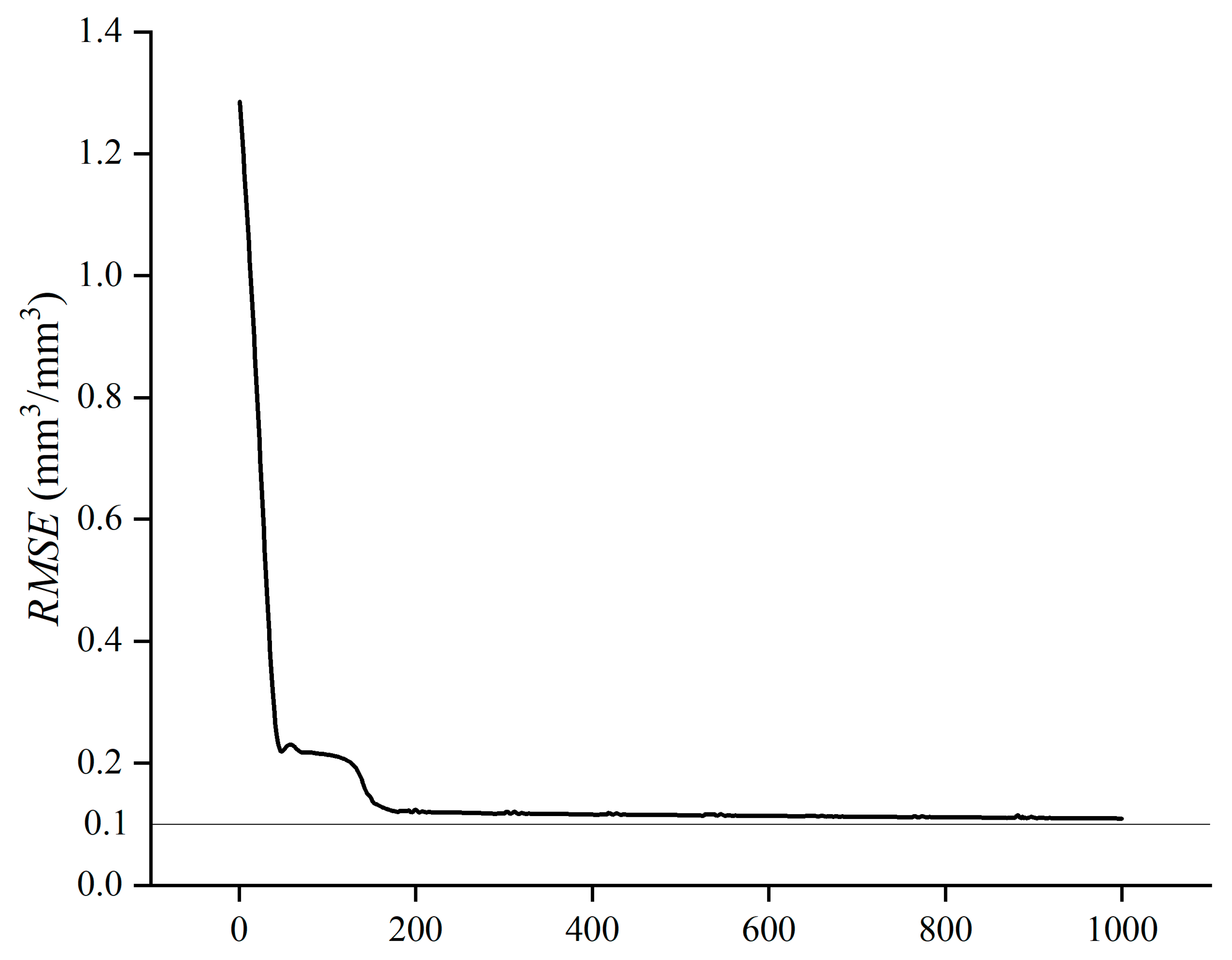
2.5.1. Back-Propagation Artificial Neural Network

The BPANN method is a self-organizing, self-learning, and self-adaptive network system [28]. It has the ability to deal with the complex nonlinear relationships in SM simulation with high accuracy [78]. The BPANN method is formed by input layers, hidden layers, and output layers [79]. As shown in Figure 2, the nodes in the input layer are the SMAP product ($S{M}_{SMAP}$), the CLM5.0 simulations ($S{M}_{CLM5.0}$), and the land surface soil temperature ($LST$) at daily interval.

According to Hornik’s equation [80], there are 6 hidden layers and 5 nodes in each layer in this study. The i-th node in the l-th hidden layer is expressed as $O_i^l$ (i = 1, 2, …,5, and l= 1, 2, …,6). For layer l + 1, the j-th node $O_j^{l+1}={{\displaystyle \sum }}_{i=1}^6{\omega }_{ij}{O}_i^l$, the weight ${\omega }_{ij}$ was allocated through Logsig nonlinear activation function. The output is the fused SM data ($S{M}_{BPANN}$) at daily interval, which was calculated by the Purelin function based on the nodes in the sixth hidden layer.

At each site, all the data were divided into training set and test set with a data ratio of 2:1, which balance the effectiveness and time consumption [24]. During the training process, the weights of the BPANN method was adjusted by back-propagation according to the acceptable error of 0.1 mm³/mm³ and learning rate of 0.01 [81]. As shown in Figure 3, the iteration number of training process is 1000 in this study.

2.5.2. Ensemble Kalman Filter

The EnKF is not only a classic method in handling nonlinear relationships, but is also specifically designed for large, high-dimensional data sets [82,83]. This makes it a highly effective filter method. Unlike traditional statistical methods, the EnKF is capable of addressing the issue of background errors changing over time by representing them as sets rather than point estimates [84]. This feature makes it particularly suitable for non-linear data sets with significant variability [85]. Moreover, this method effectively ensures the representativeness of the samples using the Gaussian distribution, which reduces computation costs and leads to more accurate results [86]. The efficiency of the EnKF method in SM estimation has been well demonstrated [87].

In this study, we propose a set of representative EnKF schemes based on multi-source data, aiming for SM estimation. The $S{M}_{SMAP}$, $S{M}_{CLM5.0}$, and $LST$ data at daily intervals were used as the input. First, we use multiple non-homogeneous equations as the conversion function between the coefficients and SM. As shown in

Table 1. The correlation coefficient (R) of $S{M}_{CRNS}$ and the $S{M}_{SMAP}$, $S{M}_{CLM5.0}$, $LST$.

	$\mathit{S}{\mathit{M}}_{\mathit{C}\mathit{L}\mathit{M}5.0}$		$\mathit{S}{\mathit{M}}_{\mathit{S}\mathit{M}\mathit{A}\mathit{P}}$		$\mathit{L}\mathit{S}\mathit{T}$
	At AGS	At DGS	At AGS	At DGS	At AGS	At DGS
$\mathrm{y}=\mathrm{ax}+\mathrm{b}$	0.371	0.656	0.573	0.566	0.154	0.328
$\mathrm{y}=\mathrm{a}{x}^2+\mathrm{b}$	0.372	0.658	0.605	0.588	0.140	0.330
$\mathrm{y}=\mathrm{a}{x}^3+\mathrm{b}$	0.374	0.661	0.605	0.588	0.109	0.304
$\mathrm{y}=\mathrm{a}{x}^4+\mathrm{b}$	0.377	0.661	0.607	0.587	0.156	0.319
$\mathrm{y}=\mathrm{a}{e}^x$	0.366	0.640	0.579	0.552	0.033	0
$\mathrm{y}=\mathrm{aln}\left(\mathrm{x}\right)$	0.369	0.639	0.562	0.523	0.037	0.330
$\mathrm{y}=\mathrm{a}{x}^b$	0.364	0.657	0.569	0.522	0.037	0

, we determine the suitable regression equation of the $S{M}_{SMAP}$, $S{M}_{CLM5.0}$, and $LST$, respectively [88]. Considering the computation costs and update rate, the suitable fitting equation is determined by Equation (1) below.

$$S{M}_{EnKF}=a_{1}S{M}_{SMAP}^2+a_{2}S{M}_{CLM5.0}+a_{3}LST+a_4$$

(1)

After determining the form of the function, a set of data from the first three months, $X=\{x_1$, $x_2$, $x_3$,…,$x_{91}\}$ is used for multiple regression, where $x_i=\{S{M}_{SMAP,i}$, $S{M}_{CLM5.0,\mathrm{i}}$, $LS{T}_{\mathrm{i}}\}$, dependent variable $Y=\{S{M}_{CRNS,1}$, $S{M}_{CRNS,2}$, $S{M}_{CRNS,3}$, $S{M}_{CRNS,4}$,…,$S{M}_{CRNS,91}\}$. The coefficient set $\overline{A}=\left\{\overline{a_1},\overline{a_2}, \overline{a_3}, \overline{a_4}\right\}$ obtained after regression is used as the true value of the state variable in the method, and a disturbance with a mean of 0 and a variance of 0.0001 is applied to make it a set that conforms to the Gaussian distribution, which is a result of our experiment, generating the state variable ${\tau }_1=\left\{A_1, A_2, A_3, A_4,\dots , A_{91}\right\}$ of the EnKF, where $A_i=\left\{a_{1,i}, a_{2,i}, a_{3,i}, a_{4,i}\right\}$.

Then, iterative calculations were performed. For iteration m, the following was undertaken: 1) The fused result $S{M}_{EnKF}=H_m^T\cdot {\overline{\tau }}_m$, was obtained based on the mean value ${\overline{\tau }}_m$, which obtained from the set of state variables ${\tau }_m$ at the time $m$, and the observation matrix $H_m$, which is composed of $S{M}_{SMAP,m}$, $S{M}_{CLM5.0,m}$, and $LS{T}_m$ at the time $m$. 2) After obtaining the observed value of the CRNS $(S{M}_{CRNS,m}$) at the time $m$, the state variables ${\tau }_{m+1}$ at the time $m+1$ was iteratively calculated ${\tau }_{m+1}={\tau }_m+K_m\left[S{M}_{CRNS,m}-H_m^T{\tau }_m\right]$, $K_m$ is the Kalman Gain matrix, which is calculated by Equations (2) and (3).

$$K_m=P_m{H}_m^T{(H_m{P}_m{H}_m^T+R)}^{-1}$$

(2)

$$P_m=\frac{1}{N}{\displaystyle \sum }_{i=1}^N\left({\tau }_m-{\overline{\tau }}_m\right){({\tau }_m-{\overline{\tau }}_m)}^T$$

(3)

The iteration numbers of loop at the DGS and the AGS are 642 and 149, respectively.

2.6. Evaluation Indices

In order to fairly compared with previous evaluation results, five statistical indices, the correlation coefficient(R) (Equation (4)), the Root-Mean-Square Errors (RMSE) (Equation (5)), the mean BIAS (BIAS) (Equation (6)), the Coefficient of Variation (CV) (Equation (7)), and the RMSE-Observations Standard Deviation Ratio (RSR) (Equation (8)) were applied to examine the performance of the different SM data sets. The equations are as follows [89,90,91]:

$$R=\frac{{{\displaystyle \sum }}_{i=1}^N\left(S{M}_i^{obs}-{\overline{SM}}^{obs}\right)\left(S{M}_i^{*}-{\overline{SM}}^{*}\right)}{\sqrt{{{\displaystyle \sum }}_{i=1}^N{\left(S{M}_i^{obs}-{\overline{SM}}^{obs}\right)}^2}\sqrt{{{\displaystyle \sum }}_{i=1}^N{\left(S{M}_i^{*}-{\overline{SM}}^{*}\right)}^2}}$$

(4)

$$RMSE=\sqrt{\frac{1}{N}{{\displaystyle \sum }}_{i=1}^N{\left(S{M}_i^{obs}-S{M}_i^{*}\right)}^2}$$

(5)

$$BIAS=\frac{1}{N}{\displaystyle \sum }_{\mathrm{i}=1}^N\left(S{M}_i^{obs}-S{M}_i^{*}\right)$$

(6)

$$CV=\frac{\sqrt{\frac{1}{N}{{\displaystyle \sum }}_{i=1}^N{\left(S{M}_i^{obs}-S{M}_i^{0bs}\right)}^2}}{{\overline{SM}}^{obs}}$$

(7)

$$RSR=\frac{\sqrt{{{\displaystyle \sum }}_{i=1}^N{\left(S{M}_i^{obs}-S{M}^{*}\right)}^2}}{\sqrt{{{\displaystyle \sum }}_{i=1}^N{\left(S{M}_i^{obs}-{\overline{SM}}^{obs}\right)}^2}}$$

(8)

where, $S{M}_i^{obs}$ is the observed SM data, which is the observed CRNS data. $S{M}_i^{*}$ is the certain SM data from the SMAP product, the CLM5.0 simulations, the fused data by BPANN (FD-BPANN), and the fused data by EnKF (FD-EnKF), respectively. ${\overline{SM}}^{obs}$ and ${\overline{SM}}^{*}$ are the average values of $S{M}_i^{obs}$ and $S{M}_i^{*}$, while N is the data number during the evaluation period. The larger R and smaller RMSE, RSR, CV, and absolute BIAS, the better the performance of the evaluated SM data sets [2].

3. Results

3.1. Evaluation of Surface Soil Moisture by the CLM5.0 Simulations and the SMAP Product against the CRNS

The simulated surface SM data from the SMAP product and the CLM5.0 simulations were evaluated against the CRNS observation. For the CLM5.0 simulations, the DGS has an R value of 0.656 (p < 0.01), RMSE of 0.046 mm³/mm³, and BIAS of 0.028 mm³/mm³ (Figure 4a). Specifically, the BIAS values of the CLM5.0 simulations in 2017, 2018, and 2019 were 0.006 mm³/mm³, 0.028 mm³/mm³, and 0.051 mm³/mm³, respectively. Although the 2019 simulations led to a slight overestimation of the overall results, the CLM5.0 simulations at the DGS captured the temporal variation trend of the observed SM. Meanwhile, the CLM5.0 simulations at the AGS has an R value of 0.372 (p < 0.01), RMSE of 0.101 mm³/mm³ and BIAS of 0.095 mm³/mm³ (Figure 4b). Results indicate that the CLM5.0 simulations at the AGS also reflected the temporal variation trend of the observed SM, but there was a significant overestimation. In summary, the CLM5.0 simulations are generally reasonable at both sites, however, perform better at the DGS than at the AGS.

The SMAP product at the DGS has an R value of 0.618 (p < 0.01), RMSE of 0.042 mm³/mm³, and BIAS of 0.025 mm³/mm³ (Figure 4c), reflecting the temporal variation trend of the measured SM, but there is a slight overestimation. The SMAP product at the AGS has an R value of 0.593 (p < 0.01), RMSE of 0.182 mm³/mm³, and BIAS of −0.180 mm³/mm³ (Figure 4d), is able to reproduce the temporal variation trend of the measured SM. We subtracted the deviation value of 0.180 mm³/mm³ from the original SMAP product to remove the systematic BIAS at the AGS and the corrected SMAP product has a new RMSE of 0.031 mm³/mm³ and BIAS of 0.001 mm³/mm³ (Figure 4d). Overall, the SMAP product is reliable at the DGS with a minor overestimation and the bias-corrected SMAP product is more suitable for the AGS since the systematic underestimation at the AGS can be significantly improved through systematic error correction.

In summary, both the CLM5.0 simulations and the SMAP product performed better at the DGS than at the AGS and showed similar performances at the DGS with similar R, RMSE, and BIAS values, while the bias-corrected SMAP product at the AGS has similar R values, higher RMSE, and BIAS values compared with the CLM5.0 simulations.

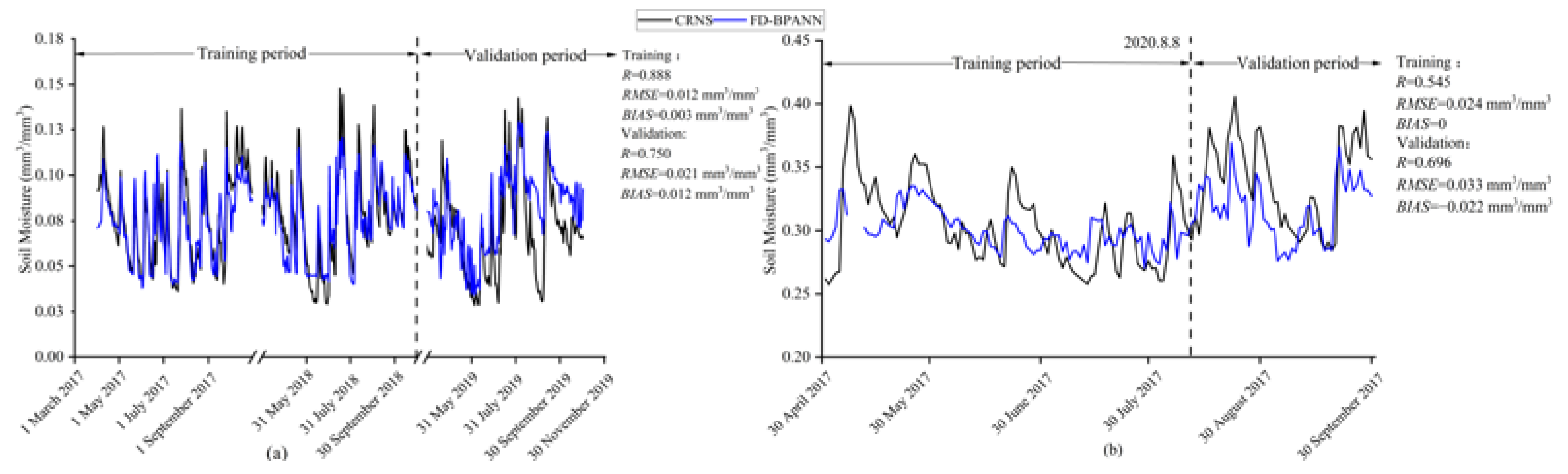
3.2. The Performance of the Fused Data by BPANN

At the DGS, the FD-BPANN performed well with the R value of 0.888, RMSE value of 0.012 mm³/mm³, and BIAS value of 0.003 mm³/mm³ in the training period, and R value of 0.750, RMSE value of 0.021 mm³/mm³, and BIAS value of 0.012 mm³/mm³ in the validation period (Figure 5a). In both periods, the FD-BPANN performed better than the CLM5.0 simulations and the SMAP product with significantly higher R values, as well as lower RMSE and BIAS values. At the AGS, the FD-BPANN performed well with the R value of 0.545, RMSE value of 0.024 mm³/mm³, and BIAS value of 0 mm³/mm³ in the training period, and R value of 0.696, RMSE value of 0.033 mm³/mm³, and BIAS value of 0.022 mm³/mm³ in the validation period (Figure 5b). In both periods, the FD-BPANN performed better than the CLM5.0 simulations with significantly larger R values, and smaller RMSE and BIAS values, and showed better performance than the SMAP product with similar R values, and smaller RMSE and BIAS values.

Comparing with the SMAP product, the FD-BPANN at the DGS improved by 44% and 71% for the R and RMSE in the training period, respectively, whereas the R decreased by 8% and RMSE improved by 87% at the AGS (

Table 2. The improvement of the fused data by BPANN (FD-BPANN) at the degraded grassland site (DGS) and the alpine grassland site (AGS).

	At the Degraded Grassland Site				At the Alpine Grassland Site
	Training Period		Validation Period		Training Period		Validation Period
	SMAP~FD-BPANN	CLM5.0~FD-BPANN	SMAP~FD-BPANN	CLM5.0~FD-BPANN	SMAP~FD-BPANN	CLM5.0~FD-BPANN	SMAP~FD-BPANN	CLM5.0~FD-BPANN
R	44% (0.618~0.888)	35% (0.656~0.888)	21% (0.618~0.750)	14% (0.656~0.750)	−8% (0.593~0.545)	47% (0.372~0.545)	17% (0.593~0.696)	87% (0.372~0.696)
RMSE (mm3/mm3)	71% (0.042~0.012)	74% (0.046~0.012)	50% (0.042~0.021)	54% (0.046~0.021)	87% (0.182~0.024)	76% (0.101~0.024)	82% (0.182~0.033)	67% (0.101~0.033)

). In the validation period, the R and RMSE of the FD-BPANN improved by 21% and 50%, respectively, at the DGS, whereas the R and RMSE of the FD-BPANN improved by 17% and 82%, respectively, at the AGS. Therefore, compared with the SMAP product, the performance improvement of the FD-BPANN at the DGS is significantly lower than at the AGS. Compared with the CLM5.0 simulations, the FD-BPANN at the DGS improved by 35% and 74% for the R and RMSE in the training period, respectively, while the two values at the AGS improved by 47% and 76%, respectively. In the validation period, the FD-BPANN at the DGS improved by 14% and 54% for the R and RMSE, respectively, while the two values at the AGS improved by 87% and 67%, respectively. Therefore, compared with the CLM5.0 simulations, the improvement of the performance of the FD-BPANN is significantly lower at the DGS than at the AGS.

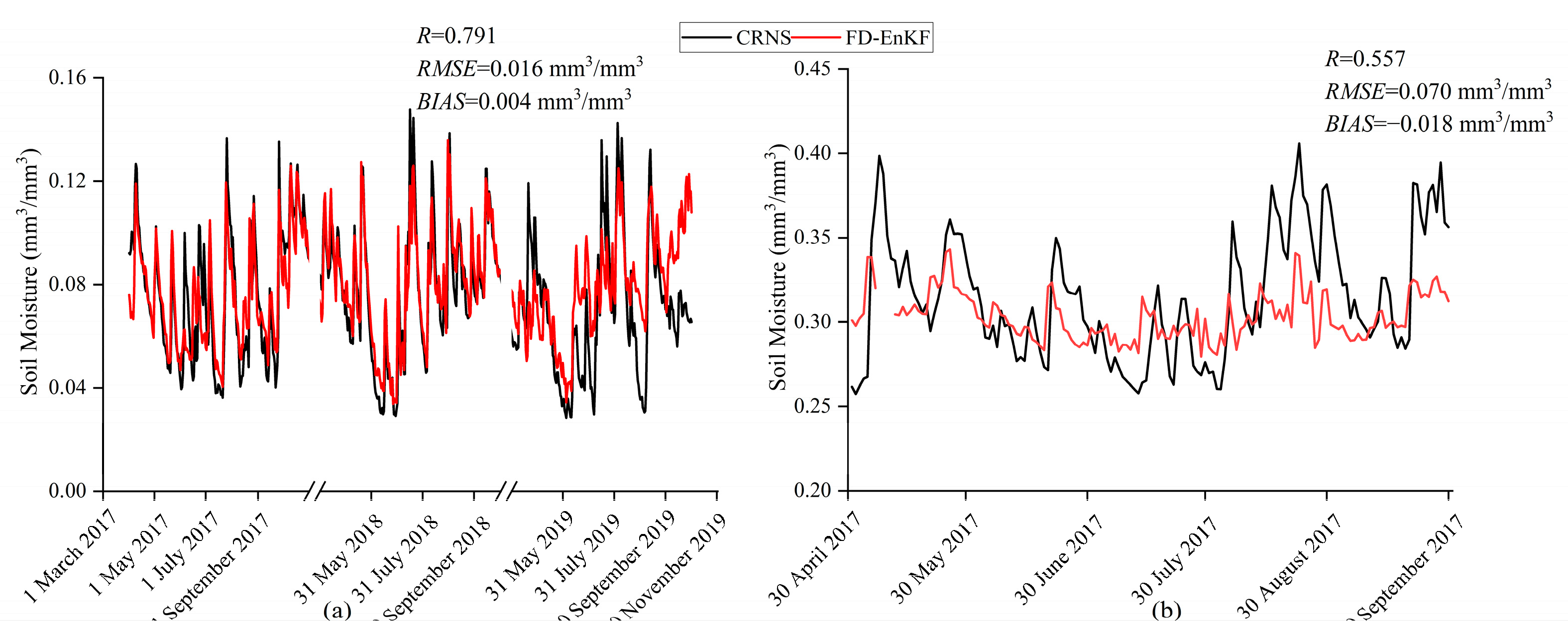
3.3. The Performance of the Fused Data by EnKF

At the DGS, the FD-EnKF performed well with an R value of 0.791, RMSE value of 0.016 mm³/mm³, and BIAS value of 0.004 mm³/mm³ (Figure 6a). It performed better than the CLM5.0 simulations and the SMAP product with significant higher R values, and lower RMSE and BIAS values. At the AGS, the FD-EnKF performed well with an R value of 0.557, RMSE value of 0.070 mm³/mm³, and BIAS value of −0.018 mm³/mm³ (Figure 6b). It performed better than the CLM5.0 simulations with significant higher R values, and lower RMSE and BIAS values, and showed better performance than the SMAP product with similar R values and lower RMSE and BIAS values.

Compared with the SMAP product, the FD-EnKF at the DGS improved by 28% and 62% for the R and RMSE, respectively, whereas the R decreased by 6% and RMSE increased by 62% at the AGS (

Table 3. The improvement of the fused data by EnKF (FD-EnKF) at the DGS and the AGS.

	At the Degraded Grassland Site		At the Alpine Grassland Site
	SMAP~FD-EnKF	CLM5.0~FD-EnKF	SMAP~FD-EnKF	CLM5.0~FD-EnKF
R	28% (0.618~0.791)	20% (0.656~0.791)	−6% (0.593~0.557)	50% (0.372~0.557)
RMSE (mm3/mm3)	62% (0.042~0.016)	65% (0.046~0.016)	62% (0.182~0.070)	31% (0.101~0.070)

). Therefore, compared with the SMAP product, the performance improvement of the FD-EnKF at the DGS is more significant than at the AGS. Compared with the CLM5.0 simulations, the FD-EnKF at the DGS improved by 20% and 65% for the R and RMSE, while these two values at the AGS improved by 50% and 31%, respectively. In summary, compared with the CLM5.0 simulations, the improvement of the performance of the FD-EnKF is not as obvious at the DGS as at the AGS.

3.4. Comparison of the Fused Data by BPANN and EnKF

As shown in Figure 5 and Figure 6, at the DGS, the FD-BPANN performed better than the FD-EnKF with higher R values, lower RMSE and BIAS values in the training periods, and similar performance in the validation period. At the AGS, the FD-BPANN performed better than the FD-EnKF with similar R values, lower RMSE and BIAS values in the training period, and with higher R values, lower RMSE values, and similar BIAS values in the validation period.

To better understand the differences of the fused data products in different SM ranges, two percentile points of SM, Q25 (25th percentile, lower SM values) and Q75 (75th percentile, higher SM values), were used to divide the SM ranges into three percentile series. The Q25 and Q75 are 0.028 mm³/mm³ and 0.092 mm³/mm³ at the AGS, and 0.286 mm³/mm³ and 0.339 mm³/mm³ at the DGS. At the DGS, the FD-BPANN performed better for higher SM data with increasing R values and similar RMSE values (Figure 7a,b) and also better than the CLM5.0 simulations and the SMAP product with higher R values and lower RMSE values in all the three ranges (Figure 7a,b). At the AGS, the FD-BPANN performed better in range ≥Q75 with R values passing the significant test of 0.01 (Figure 7c,d). In ranges of <Q25 and Q25–Q75, the FD-BPANN showed worse performance than in range ≥Q75 with similar RMSE and lower R values.

At the DGS, the FD-EnKF performed best in range ≥Q75 with the highest R values, followed by R values in the range <Q25 and the range Q25–Q75, with similar RMSE values in all the ranges (Figure 7a,b). The FD-EnKF performed better than the CLM5.0 simulations and the SMAP product with higher R values and lower RMSE values in all the three ranges (Figure 7a,b). At the AGS, the FD-EnKF performed better in range ≥Q75 with R values passing the significant test of 0.01 (Figure 7c,d). In ranges of <Q25 and Q25–Q75, the FD-EnKF showed worse performance than in range ≥Q75 with similar RMSE and lower R values.

As shown in Figure 7, in the range <Q25, the FD-BPANN has smaller R values and similar RMSE values compared with the FD-EnKF at the DGS, and similar R and RMSE values at the AGS. It indicates a better performance of the FD-EnKF than the FD-BPANN in the range <Q25. However, in the ranges of Q25~Q75 and ≥Q75, the FD-BPANN has higher R and similar RMSE values at the DGS, and similar or higher R values and lower RMSE values at the AGS. Thus, the performance of the FD-BPANN is better than the FD-EnKF in the ranges of Q25–Q75 and ≥Q75.

4. Discussion

4.1. The Impact of Different Method Mechanisms on Data Fusion

The performance of the FD-BPANN is better than that of the FD-EnKF at both the DGS and AGS, because of different method mechanisms of the BPANN and EnKF methods. The EnKF firstly determines the optimal fitting equation, and then iteratively updates the set of state variables with additional data sets [36,92]. Its performance is determined by the variability of the SMAP product, the CLM5.0 simulations, and the CRNS observations [30]. As shown in

Table 4. The coefficient of variation (CV) of three data sets at the DGS and the AGS.

	The Degraded Grassland Site	The Alpine Grassland Site
The CRNS	34%	11%
The CLM5.0 simulations	46%	4%
The SMAP product	42%	10%

, the CV values of the SMAP product, the CLM5.0 simulations, and the CRNS observations are 42%, 46%, and 34% at DGS, and 10%, 4%, and 11% at AGS, respectively. All of them showed strong variability [93]. To be more specific, the absolute difference values between $S{M}_{CRNS}$ at two adjacent days are shown in Figure 8, indicating strong variability of $S{M}_{CRNS}$. As a result, the FD-EnKF has a worse performance.

The BPANN method is based on an iterative gradient descent training procedure, and the trained BPANN assigned higher weights to the data set with better performance [37]. The weights were determined through back-propagation learning process with 1000 iterations in this study. As shown in

Table 5. The weights of the SMAP product and the CLM5.0 simulations in the five nodes of the BPANN at both sites.

	Node1		Node2		Node3		Node4		Node5
	At the DGS	At the AGS	At the DGS	At the AGS	At the DGS	At the AGS	At the DGS	At the AGS	At the DGS	At the AGS
The weights of the SMAP product	−5.311	7.166	−1.588	5.936	−6.704	7.269	−7.630	−9.663	−5.782	5.955
The weights of the CLM5.0 simulations	7.906	2.679	−6.477	7.274	5.358	0.113	5.656	−0.637	6.693	4.929

, the absolute weight values of the CLM5.0 simulations were higher than that of the SMAP product at the DGS, and lower than that of the SMAP product at the AGS. Meanwhile, the CLM5.0 simulations showed better performance than the SMAP product at the DGS and worse performance than the SMAP product at the AGS. Thus, the BPANN adjusted higher weights to inputs with better performance through self-organization and self-learning [41,46], leading to a better performance of the FD-BPANN.

In addition, the FD-BPANN performed worse than the FD-EnKF in the range <Q25, although it showed a better overall performance. This is because the adopted gradient descent algorithm of the BPANN method makes it tend to be trapped in a local minimum and ignore the overall minimum value, which caused the overestimation of the FD-BPANN [37].

4.2. Applicability of the BPANN and the EnKF in Different Climatic Zones

To fairly compare the performance of the BPANN method in different areas, this study summarized results and further calculated the RSR values of the previous studies [38,40,41,75,94,95,96]. As shown in

Table 6. The performance of the fused data in previous studies.

Study Area	Area	Soil	Topography Types	Data	Method	R	RMSE (mm3/mm3)	Reference
Solani river catchment in India	humid area	sandy loam soil	flat alluvial areas	ERS-2 SAR	BPANN	0.837~0.900	0.055~0.089	[38]
Tibetan Plateau	semi-humid area	sand and silty	plateau and mountain	The Fengyun-3B Microwave Radiation Imager soil moisture product	BPANN	0.748~0.872	0.060~0.100	[40]
Varanasi in India	humid area	\	plain	Ground based bistatic scatterometer data at X-band	BPANN	\	0.010~0.013	[41]
Yanco area, Murrumbidgee River catchment	arid and semi-arid area	\	flood plain	The Murrumbidgee Soil Moisture Monitoring Network, The Soil Moisture Active Passive Experiments (SMAPEx) airborne observations, MODIS LST and NDVI products	ANN	\	0.060~0.140	[75]
Goulburn Catchment in southeastern Australia	humid area	clay soil	flat alluvial areas	The National Airborne Field Experiment 2005 (NAFE’05) data	BPANN	0.830~0.890	0.037~0.058	[94]
Mainland China	all	\	\	EchDemoSat-1 and CYGNSS Data	BPANN	0.850~0.933	0.059~0.087	[95]
Taihu Lake basin of China	humid area	loam soil	plain	Rainfall, evaporation, temperature, humidity, and wind speed	BPANN	0.840~0.872	0.013~0.015	[96]
Degraded grassland site; Alpine grassland site	semi-arid area	sandy soil and silt loam	plateau and mountain	Community Land Model 5.0 (clm5.0); The Soil Moisture Active and Passive (SMAP)	BPANN	0.545–0.888	0.012–0.033	This study

, for the BPANN method, the ranges of R, RMSE, and RSR are 0.830–0.900, 0.013–0.089 mm³/mm³, and 0.149–0.470 in the humid area, respectively. In the semi-humid area, the ranges of R, RMSE, and RSR are 0.641–0.948, 0.060–0.100 mm³/mm³, and 0.477–0.542, respectively. In the arid and semi-arid areas, R value ranges from 0.850 to 0.933, RMSE value ranges from 0.059 to 0.087 mm³/mm³, and RSR value is about 1.125. Overall, the BPANN method performed better in humid areas, then followed by semi-humid areas, and finally arid and semi-arid areas. Moreover, compared with the previous studies in arid and semi-arid areas, the FD-BPANN in this study performed better with similar R, and smaller RMSE and RSR values. This is because the CRNS data were applied as observations in this study, which partially avoids the impacts of scale mismatching.

Furthermore, previous studies showed that the NSE value of the EnKF method in the semi-humid area is 0.902 [23], while the NSE values are 0.602 and 0.739 at the DGS and the AGS, respectively. Therefore, the performance of the EnKF method in this study is credible.

As shown in Table 6, regarding the topographic attributes, the BPANN performed better in plains and flat alluvial areas than in plateaus and mountains. This is because the SM showed stronger variability in plateaus and mountains than plains and flat alluvial areas.

As for the soil type, the BPANN method performed better on loam and clay, then followed by sandy loam, and finally sand and silt. The particle size and porosity of soil significantly influence the vertical permeability of soil. As a result, the bigger particle size and porosity of soil lead to the faster transfer of surface water to the deeper water table, which results in stronger variability of SM. Therefore, we find that bigger particle size and porosity of soil leads to worse performance of the BPANN method. In addition, the poorer observed correlation can also be partly explained by the fact that the time sampling of the data is one day long and has difficulty in capturing these rapid changes in SM.

In addition, from the Table 2 and Table 3, we found that data fusion is more meaningful in the mountainous area with poor performance of the data sets, because compared with the original data sets, the performance improvements of both the FD-BPANN and the FD-EnKF are more significant at the AGS than at the DGS. Compared with previous research results, the BPANN method is more suitable for mountainous area with strong SM variations and poor observation data sets [94,97,98].

5. Conclusions

This study compared the performance of the EnKF and BPANN methods in data fusion against the CRNS observations in data-lacking, heterogeneous grasslands in northwestern China. The main conclusions of our study are as follows.

Compared with the original data sets at both sites, the RMSE of the FD-BPANN and FD-EnKF improved by more than 50% and 31%, respectively. The performance improvement of the FD-BPANN at the DGS is significantly lower than at the AGS. The FD-EnKF, however, showed the opposite result.

The performance of the FD-BPANN is better than that of the FD-EnKF. This is because the BPANN method assigned higher weights to input data with better performance through self-organization and self-learning, but the EnKF method is affected by the strong variabilities of both the input data and the output observations. However, the FD-BPANN showed worst performance with overestimations in the low SM range of 25th percentile (<Q25). Because the BPANN method is based on an iterative gradient descent training procedure, this makes it tend to be trapped in a local minimum.

The BPANN method performed better in humid areas, then followed by semi-humid areas, and finally arid and semi-arid areas. The better performance of the BPANN method in this study than the previous studies is because the scale-mismatch is partially avoided by the CRNS observations. Meanwhile, the BPANN method is more suitable for mountainous area with strong SM variations and poor observation data sets.

The above results provide insights for estimating SM data at large scales, and thus support related climatic, hydrological and ecohydrological research. Nevertheless, due to the limited number of in situ observation sites, this study only focused on the comparison of the BPANN and the EnKF on grasslands in semi-arid areas. Future research needs to evaluate the applicability of both methods under diverse climatic and environmental conditions in estimating SM at large scales. The big differences in spatial resolutions of the SM products may produce big uncertainty to the result. Spatial downscaling has recently become a crucial process in the regional application of coarse resolution SM products, which greatly alleviates the spatial uncertainty for surface soil moisture. Therefore, future study will use the fusion methods with the downscaled data sets [99,100,101]

References

1. Ren, X.; Zhang, P.; Chen, X.; Guo, J.; Jia, Z. Effect of Different Mulches under Rainfall Concentration System on Corn Production in the Semi-arid Areas of the Loess Plateau. Sci. Rep. 2016, 6, 19019. [Google Scholar] [CrossRef] [Green Version]
2. Zhang, L.; He, C.; Zhang, M. Multi-Scale Evaluation of the SMAP Product Using Sparse In-Situ Network over a High Mountainous Watershed, Northwest China. Remote Sens. 2017, 9, 1111. [Google Scholar] [CrossRef] [Green Version]
3. Alsafadi, K.; Bi, S.; Bashir, B.; Mohammed, S.; Sammen, S.S.; Alsalman, A.; Srivastava, A.K.; El Kenawy, A. Assessment of Carbon Productivity Trends and Their Resilience to Drought Disturbances in the Middle East Based on Multi-Decadal Space-Based Datasets. Remote Sens. 2022, 14, 6237. [Google Scholar] [CrossRef]
4. Huang, C.; Chen, W.; Li, Y.; Shen, H.; Li, X. Assimilating multi-source data into land surface model to simultaneously improve estimations of SM, soil temperature, and surface turbulent fluxes in irrigated fields. Agric. For. Meteorol. 2016, 230–231, 142–156. [Google Scholar] [CrossRef] [Green Version]
5. Wang, X.; Sun, G.; Jia, Y.; Li, F.; Xu, J. Crop yield and soil water restoration on 9-year-old alfalfa pasture in the semiarid Loess Plateau of China. Agric. Water Manag. 2008, 95, 190–198. [Google Scholar] [CrossRef]
6. Brocca, L.; Melone, F.; Moramarco, T.; Wagner, W.; Hasenauer, S. ASCAT soil wetness index validation through in situ and modeled soil moisture data in central Italy. Remote Sens. Environ. 2010, 114, 2745–2755. [Google Scholar] [CrossRef]
7. Brown, M.E.; Escobar, V.M. Assessment of Soil Moisture Data Requirements by the Potential SMAP Data User Community: Review of SMAP Mission User Community. IEEE J.-Stars. 2014, 7, 277–283. [Google Scholar] [CrossRef]
8. Wang, Y.; Sun, H.; Zhao, Y. Characterizing spatial-temporal patterns and abrupt changes in deep soil moisture across an intensively managed watershed. Geoderma 2019, 341, 181–194. [Google Scholar] [CrossRef]
9. Zheng, J.; Zhao, T.; Lü, H.; Shi, J.; Cosh, M.H.; Ji, D.; Jiang, L.; Cui, Q.; Lu, H.; Yang, K.; et al. Assessment of 24 soil moisture datasets using a new in situ network in the Shandian River Basin of China. Remote Sens. Environ. 2022, 271, 112891. [Google Scholar] [CrossRef]
10. Yi, C.; Li, X.; Zeng, J.; Fan, L.; Xie, Z.; Gao, L.; Xing, Z.; Ma, H.; Boudah, A.; Zhou, H.; et al. Assessment of five SMAP soil moisture products using ISMN ground-based measurements over varied environmental conditions. J. Hydrol. 2023, 619, 129325. [Google Scholar] [CrossRef]
11. Shin, Y.; Mohanty, B.P.; Kim, J.; Lee, T. Multi-model based soil moisture simulation approach under contrasting weather conditions. J. Hydrol. 2023, 617, 129112. [Google Scholar] [CrossRef]
12. Gao, X.; Avramov, A.; Saikawa, E.; Schlosser, C.A. Emulation of Community Land Model Version 5 (CLM5) to Quantify Sensitivity of Soil Moisture to Uncertain Parameters. J. Hydrometeorol. 2021, 22, 259–278. [Google Scholar] [CrossRef]
13. Crow, W.T.; Berg, A.A.; Cosh, M.H.; Loew, A.; Mohanty, B.P.; Panciera, R.; de Rosnay, P.; Ryu, D.; Walker, J.P. Upscaling sparse ground-based soil moisture observations for the validation of coarse-resolution satellite soil moisture products. Rev. Geophys. 2012, 50, 372. [Google Scholar] [CrossRef] [Green Version]
14. Gumuzzio, A.; Brocca, L.; Sánchez, N.; González-Zamora, A.; Martínez-Fernández, J. Comparison of SMOS, modelled andin situlong-term soil moisture series in the northwest of Spain. Hydrolog. Sci. J. 2016, 61, 2610–2625. [Google Scholar] [CrossRef] [Green Version]
15. Bindlish, R.; Jackson, T.; Cosh, M.; Tianjie, Z.; O’Neill, P. Global Soil Moisture From the Aquarius/SAC-D Satellite: Description and Initial Assessment. IEEE Geosci. Remote Sens. 2015, 12, 923–927. [Google Scholar] [CrossRef]
16. Kim, S.; Liu, Y.Y.; Johnson, F.M.; Parinussa, R.M.; Sharma, A. A global comparison of alternate AMSR2 soil moisture products: Why do they differ? Remote Sens. Environ. 2015, 161, 43–62. [Google Scholar] [CrossRef]
17. Peng, J.; Albergel, C.; Balenzano, A.; Brocca, L.; Cartus, O.; Cosh, M.H.; Crow, W.T.; Dabrowska-Zielinska, K.; Dadson, S.; Davidson, M.W.J.; et al. A roadmap for high-resolution satellite soil moisture applications—Confronting product characteristics with user requirements. Remote Sens. Environ. 2021, 252, 112162. [Google Scholar] [CrossRef]
18. Entekhabi, D.; Njoku, E.G.; O’Neill, P.E.; Kellogg, K.H.; Crow, W.T.; Edelstein, W.N.; Entin, J.K.; Goodman, S.D.; Jackson, T.J.; Johnson, J.; et al. The Soil Moisture Active Passive (SMAP) Mission. IEEE 2010, 98, 704–716. [Google Scholar] [CrossRef]
19. Zhang, L.; He, C.; Zhang, M.; Zhu, Y. Evaluation of the SMOS and SMAP soil moisture products under different vegetation types against two sparse in situ networks over arid mountainous watersheds, Northwest China. Sci. China Earth Sci. 2019, 62, 703–718. [Google Scholar] [CrossRef]
20. Peng, F.; Mu, M.; Sun, G. Evaluations of Uncertainty and Sensitivity in Soil Moisture Modeling on the Tibetan Plateau. Tellus A 2020, 72, 1704963. [Google Scholar] [CrossRef] [Green Version]
21. Lee, J.; Park, S.; Im, J.; Yoo, C.; Seo, E. Improved soil moisture estimation: Synergistic use of satellite observations and land surface models over CONUS based on machine learning. J. Hydrol. 2022, 609, 127749. [Google Scholar] [CrossRef]
22. Mahmood, H.S.; Hoogmoed, W.B.; Henten, E.J. Sensor data fusion to predict multiple soil properties. Precis. Agric. 2012, 13, 628–645. [Google Scholar] [CrossRef]
23. Srivastava, P.K.; Han, D.; Rico-Ramirez, M.A.; Al-Shrafany, D.; Islam, T. Data Fusion Techniques for Improving Soil Moisture Deficit Using SMOS Satellite and WRF-NOAH Land Surface Model. Water Resour. Manag. 2013, 27, 5069–5087. [Google Scholar] [CrossRef]
24. Wang, Z.; Mao, Z.; Xia, J.; Du, P.; Shi, L.; Huang, H.; Wang, T.; Gong, F.; Zhu, Q. Data fusion in data scarce areas using a back-propagation artificial neural network model: A case study of the South China Sea. Front. Earth Sci. 2017, 12, 280–298. [Google Scholar] [CrossRef]
25. Nagarajan, K.; Judge, J.; Graham, W.D.; Monsivais-Huertero, A. Particle Filter-based assimilation algorithms for improved estimation of root-zone soil moisture under dynamic vegetation conditions. Adv. Water Resour. 2011, 34, 433–447. [Google Scholar] [CrossRef]
26. Im, J.; Park, S.; Rhee, J.; Baik, J.; Choi, M. Downscaling of AMSR-E soil moisture with MODIS products using machine learning approaches. Environ. Earth Sci. 2016, 75, 1120. [Google Scholar] [CrossRef]
27. Mouazen, A.M.; Alhwaimel, S.A.; Kuang, B.; Waine, T. Multiple on-line soil sensors and data fusion approach for delineation of water holding capacity zones for site specific irrigation. Soil. Till Res. 2014, 143, 95–105. [Google Scholar] [CrossRef]
28. Song, Y.; Wu, W.; Liu, Z.; Yang, X.; Liu, K.; Lu, W. An Adaptive Pansharpening Method by Using Weighted Least Squares Filter. IEEE Geosci. Remote Sens. Lett. 2016, 13, 18–22. [Google Scholar] [CrossRef]
29. Zhu, Q.; Wang, Y.; Luo, Y. Improvement of multi-layer soil moisture prediction using support vector machines and ensemble Kalman filter coupled with remote sensing soil moisture datasets over an agriculture dominant basin in China. Hydrol. Process. 2021, 35, e14154. [Google Scholar] [CrossRef]
30. Houtekamer, P.L.; Zhang, F. Review of the Ensemble Kalman Filter for Atmospheric Data Assimilation. Mon. Weather. Rev. 2016, 144, 4489–4532. [Google Scholar] [CrossRef]
31. Schillings, C.; Stuart, A.M. Analysis of the Ensemble Kalman Filter for Inverse Problems. Siam J. Numer. Anal. 2017, 55, 1264–1290. [Google Scholar] [CrossRef] [Green Version]
32. Turlapaty, A.C.; Anantharaj, V.G.; Younan, N.H.; Joseph Turk, F. Precipitation data fusion using vector space transformation and artificial neural networks. Pattern Recogn. Lett. 2010, 31, 1184–1200. [Google Scholar] [CrossRef]
33. Tangdamrongsub, N.; Steele-Dunne, S.C.; Gunter, B.C.; Ditmar, P.G.; Sutanudjaja, E.H.; Sun, Y.; Xia, T.; Wang, Z. Improving estimates of water resources in a semi-arid region by assimilating GRACE data into the PCR-GLOBWB hydrological model. Hydrol. Earth Syst. Sci. 2017, 21, 2053–2074. [Google Scholar] [CrossRef] [Green Version]
34. Dai, X.; Huo, Z.; Wang, H. Simulation for response of crop yield to soil moisture and salinity with artificial neural network. Field Crop Res. 2011, 121, 441–449. [Google Scholar] [CrossRef]
35. Wu, Y.-C.; Feng, J.-W. Development and Application of Artificial Neural Network. Wireless Pers. Commun. 2017, 102, 1645–1656. [Google Scholar] [CrossRef]
36. Khan, R.S.; Bhuiyan, M.A.E. Artificial Intelligence-Based Techniques for Rainfall Estimation Integrating Multisource Precipitation Datasets. Atmosphere 2021, 12, 1239. [Google Scholar] [CrossRef]
37. Yang, Z.P.; Lu, W.X.; Long, Y.Q.; Li, P. Application and comparison of two prediction models for groundwater levels: A case study in Western Jilin Province, China. J. Arid. Environ. 2009, 73, 487–492. [Google Scholar] [CrossRef]
38. Said, S.; Kothyari, U.C.; Arora, M.K. ANN-based soil moisture retrieval over bare and vegetated areas using ERS-2 SAR data. J. Hydrol. Eng. 2008, 13, 461–475. [Google Scholar] [CrossRef]
39. Pan, L.; Chen, Y.; Xu, Y.; Li, J.; Lu, H. A model for soil moisture content prediction based on the change in ultrasonic velocity and bulk density of tillage soil under alternating drying and wetting conditions. Measurement 2022, 189, 110504. [Google Scholar] [CrossRef]
40. Cui, Y.; Long, D.; Hong, Y.; Zeng, C.; Zhou, J.; Han, Z.; Liu, R.; Wan, W. Validation and reconstruction of FY-3B/MWRI soil moisture using an artificial neural network based on reconstructed MODIS optical products over the Tibetan Plateau. J. Hydrol. 2016, 543, 242–254. [Google Scholar] [CrossRef]
41. Gupta, D.K.; Prasad, R.; Kumar, P.; Vishwakarma, A.K. Soil moisture retrieval using ground based bistatic scatterometer data at X-band. Adv. Space Res. 2017, 59, 996–1007. [Google Scholar] [CrossRef]
42. Yuan, Q.; Li, S.; Yue, L.; Li, T.; Shen, H.; Zhang, L. Monitoring the Variation of Vegetation Water Content with Machine Learning Methods: Point–Surface Fusion of MODIS Products and GNSS-IR Observations. Remote Sens. 2019, 11, 1440. [Google Scholar] [CrossRef] [Green Version]
43. Berdugo, M.; Delgado-Baquerizo, M.; Soliveres, S.; Hernandez-Clemente, R.; Zhao, Y.; Gaitan, J.; Gross, N.; Saiz, H.; Maire, V.; Lehman, A.; et al. Global ecosystem thresholds driven by aridity. Science 2020, 367, 787–790. [Google Scholar] [CrossRef] [Green Version]
44. Zhou, W.; Gang, C.; Zhou, L.; Chen, Y.; Li, J.; Ju, W.; Odeh, I. Dynamic of grassland vegetation degradation and its quantitative assessment in the northwest China. Acta Oecol. 2014, 55, 86–96. [Google Scholar] [CrossRef]
45. Lyu, S.; Wang, J.; Song, X.; Wen, X. The relationship of δD and δ18O in surface soil water and its implications for soil evaporation along grass transects of Tibet, Loess, and Inner Mongolia Plateau. J. Hydrol. 2021, 600, 126533. [Google Scholar] [CrossRef]
46. Chen, Y.; Yang, K.; Qin, J.; Zhao, L.; Tang, W.; Han, M. Evaluation of AMSR-E retrievals and GLDAS simulations against observations of a soil moisture network on the central Tibetan Plateau. J. Geophys. Res. Atmos. 2013, 118, 4466–4475. [Google Scholar] [CrossRef]
47. Zhang, L.; He, C.; Bai, X.; Zhu, Y. Physically Based Adjustment Factors for Precipitation Estimation in a Large Arid Mountainous Watershed, Northwest China. J. Hydrol. Eng. 2017, 22, 04017047. [Google Scholar] [CrossRef]
48. Tan, X.; Zhang, L.; He, C.; Zhu, Y.; Han, Z.; Li, X. Applicability of cosmic-ray neutron sensor for measuring soil moisture at the agricultural-pastoral ecotone in northwest China. Sci. China Earth Sci. 2020, 63, 1730–1744. [Google Scholar] [CrossRef]
49. Deng, M.; Meng, X.; Lyv, Y.; Zhao, L.; Li, Z.; Hu, Z.; Jing, H. Comparison of Soil Water and Heat Transfer Modeling Over the Tibetan Plateau Using Two Community Land Surface Model (CLM) Versions. J. Adv. Model. Earth Syst. 2020, 12, e2020MS002189. [Google Scholar] [CrossRef]
50. Ou, M.; Zhang, S. Evaluation and Comparison of the Common Land Model and the Community Land Model by Using In Situ Soil Moisture Observations from the Soil Climate Analysis Network. Land 2022, 11, 126. [Google Scholar] [CrossRef]
51. Xue, Y.; Zhang, B.; He, C.; Shao, R. Detecting Vegetation Variations and Main Drivers over the Agropastoral Ecotone of Northern China through the Ensemble Empirical Mode Decomposition Method. Remote Sens. 2019, 11, 1860. [Google Scholar] [CrossRef] [Green Version]
52. Wang, X.; Zhang, B.; Xu, X.; Tian, J.; He, C. Regional water-energy cycle response to land use/cover change in the agro-pastoral ecotone, Northwest China. J. Hydrol. 2020, 580, 124246. [Google Scholar] [CrossRef]
53. Li, X.; Xu, X.; Wang, X.; Xu, S.; Tian, W.; Tian, J.; He, C. Assessing the Effects of Spatial Scales on Regional Evapotranspiration Estimation by the SEBAL Model and Multiple Satellite Datasets: A Case Study in the Agro-Pastoral Ecotone, Northwestern China. Remote Sens. 2021, 13, 1524. [Google Scholar] [CrossRef]
54. Hou, Y.; Zhou, G.; Xu, Z.; Liu, T.; Zhang, X. Interactive effects of warming and increased precipitation on community structure and composition in an annual forb dominated desert steppe. PLoS ONE 2013, 8, e70114. [Google Scholar] [CrossRef] [PubMed] [Green Version]
55. Ma, Q.; Yu, H.; Liu, X.; Xu, Z.; Zhou, G.; Shi, Y. Climatic warming shifts the soil nematode community in a desert steppe. Clim. Chang. 2018, 150, 243–258. [Google Scholar] [CrossRef]
56. Ma, Q.; Liu, X.; Li, Y.; Li, L.; Yu, H.; Qi, M.; Zhou, G.; Xu, Z.; Schwinning, S. Nitrogen deposition magnifies the sensitivity of desert steppe plant communities to large changes in precipitation. J. Ecol. 2019, 108, 598–610. [Google Scholar] [CrossRef]
57. Hou, D.; He, W.; Liu, C.; Qiao, X.; Guo, K. Litter accumulation alters the abiotic environment and drives community successional changes in two fenced grasslands in Inner Mongolia. Ecol. Evol. 2019, 9, 9214–9224. [Google Scholar] [CrossRef]
58. Yang, J.-X.; Hou, D.-J.; Qiao, X.-G.; Geng, X.-M.; Guo, K.; He, W.-M. Plowing, seeding, and fertilizing differentially influence species diversity, functional groups and community productivity in a degraded steppe. Flora 2019, 257, 151414. [Google Scholar] [CrossRef]
59. Zhang, L.; He, C.; Li, J.; Wang, Y.; Wang, Z. Comparison of IDW and Physically Based IDEW Method in Hydrological Modelling for a Large Mountainous Watershed, Northwest China. River Res. Appl. 2017, 33, 912–924. [Google Scholar] [CrossRef]
60. Tian, J.; Zhang, B.; He, C.; Han, Z.; Bogena, H.R.; Huisman, J.A. Dynamic response patterns of profile soil moisture wetting events under different land covers in the Mountainous area of the Heihe River Watershed, Northwest China. Agric. For. Meteorol. 2019, 271, 225–239. [Google Scholar] [CrossRef]
61. Xu, X.; Li, X.; Wang, X.; He, C.; Tian, W.; Tian, J.; Yang, L. Estimating daily evapotranspiration in the agricultural-pastoral ecotone in Northwest China: A comparative analysis of the Complementary Relationship, WRF-CLM4.0, and WRF-Noah methods. Sci. Total Environ. 2020, 729, 138635. [Google Scholar] [CrossRef] [PubMed]
62. Kang, W.M.; Tian, J.; Lai, Y.; Xu, S.Y.; Gao, C.; Hong, W.J.; Zhou, Y.X.; Pei, L.N.; He, C.S. Occurrence and controls of preferential flow in the upper stream of the Heihe River Basin, Northwest China. J. Hydrol. 2022, 607, 127528. [Google Scholar] [CrossRef]
63. Lai, Y.; Tian, J.; Kang, W.M.; Gao, C.; Hong, W.J.; He, C.S. Rainfall estimation from surface soil moisture using SM2RAIN in cold mountainous areas. J. Hydrol. 2022, 606, 127430. [Google Scholar] [CrossRef]
64. Zhu, X.; Shao, M.A.; Jia, X.; Huang, L.; Zhu, J.; Zhang, Y. Application of temporal stability analysis in depth-scaling estimated soil water content by cosmic-ray neutron probe on the northern Tibetan Plateau. J. Hydrol. 2017, 546, 299–308. [Google Scholar] [CrossRef]
65. McJannet, D.L.; Desilets, D. Incoming Neutron Flux Corrections for Cosmic-Ray Soil and Snow Sensors Using the Global Neutron Monitor Network. Water Resour. Res. 2023, 59, e2022WR033889. [Google Scholar] [CrossRef]
66. Zreda, M.; Desilets, D.; Ferré, T.P.A.; Scott, R.L. Measuring soil moisture content non-invasively at intermediate spatial scale using cosmic-ray neutrons. Geophys. Res. Lett. 2008, 35, l035655. [Google Scholar] [CrossRef] [Green Version]
67. Desilets, D.; Zreda, M.; Ferré, T.P.A. Nature’s neutron probe: Land surface hydrology at an elusive scale with cosmic rays. Water Resour. Res. 2010, 46, W11505. [Google Scholar] [CrossRef] [Green Version]
68. Köhli, M.; Schrön, M.; Zreda, M.; Schmidt, U.; Dietrich, P.; Zacharias, S. Footprint characteristics revised for field-scale SM monitoring with cosmic-ray neutrons. Water Resour. Res. 2015, 51, 5772–5790. [Google Scholar] [CrossRef] [Green Version]
69. Zhang, W.; Li, Y.; Wu, X.; Chen, Y.; Chen, A.; Schwalm, C.R.; Kimball, J.S. Divergent Response of Vegetation Growth to Soil Water Availability in Dry and Wet Periods Over Central Asia. J. Geophys. Res. Biogeosci. 2021, 126, e2020JG005912. [Google Scholar] [CrossRef]
70. Lawrence, D.M.; Fisher, R.A.; Koven, C.D.; Oleson, K.W.; Swenson, S.C.; Bonan, G.; Collier, N.; Ghimire, B.; van Kampenhout, L.; Kennedy, D.; et al. The Community Land Model Version 5: Description of New Features, Benchmarking, and Impact of Forcing Uncertainty. J. Adv. Model Earth Syst. 2019, 11, 4245–4287. [Google Scholar] [CrossRef] [Green Version]
71. Boas, T.; Bogena, H.; Grünwald, T.; Heinesch, B.; Ryu, D.; Schmidt, M.; Vereecken, H.; Western, A.; Hendricks Franssen, H.-J. Improving the representation of cropland sites in the Community Land Model (CLM) version 5.0. Geosci. Model Dev. 2021, 14, 573–601. [Google Scholar] [CrossRef]
72. Ma, X.; Jin, J.; Zhu, L.; Liu, J. Evaluating and improving simulations of diurnal variation in land surface temperature with the Community Land Model for the Tibetan Plateau. PeerJ 2021, 9, e11040. [Google Scholar] [CrossRef] [PubMed]
73. Colliander, A.; Jackson, T.J.; Bindlish, R.; Chan, S.; Das, N.; Kim, S.B.; Cosh, M.H.; Dunbar, R.S.; Dang, L.; Pashaian, L.; et al. Validation of SMAP surface soil moisture products with core validation sites. Remote Sens. Environ. 2017, 191, 215–231. [Google Scholar] [CrossRef]
74. Ojha, N.; Merlin, O.; Suere, C.; Escorihuela, M.J. Extending the Spatio-Temporal Applicability of DISPATCH Soil Moisture Downscaling Algorithm: A Study Case Using SMAP, MODIS and Sentinel-3 Data. Front. Env. Sci. Switz. 2021, 9, 555216. [Google Scholar] [CrossRef]
75. Senanayake, I.P.; Yeo, I.Y.; Willgoose, G.R.; Hancock, G.R. Disaggregating satellite soil moisture products based on soil thermal inertia: A comparison of a downscaling model built at two spatial scales. J. Hydrol. 2021, 594, 125894. [Google Scholar] [CrossRef]
76. Nadeem, A.A.; Zha, Y.; Shi, L.; Ran, G.; Ali, S.; Jahangir, Z.; Afzal, M.M.; Awais, M. Multi-Scale Assessment of SMAP Level 3 and Level 4 Soil Moisture Products over the Soil Moisture Network within the ShanDian River (SMN-SDR) Basin, China. Remote Sens. 2022, 14, 982. [Google Scholar] [CrossRef]
77. Vereecken, H.; Huisman, J.A.; Hendricks Franssen, H.J.; Brüggemann, N.; Bogena, H.R.; Kollet, S.; Javaux, M.; van der Kruk, J.; Vanderborght, J. Soil hydrology: Recent methodological advances, challenges, and perspectives. Water Resour. Res. 2015, 51, 2616–2633. [Google Scholar] [CrossRef]
78. Yamaç, S.S.; Şeker, C.; Negiş, H. Evaluation of machine learning methods to predict soil moisture constants with different combinations of soil input data for calcareous soils in a semi-arid area. Agric. Water Manag. 2020, 234, 106121. [Google Scholar] [CrossRef]
79. Wang, S. Multisensor data fusion of motion monitoring system based on BP neural network. J. Supercomput. 2019, 76, 1642–1656. [Google Scholar] [CrossRef]
80. Hornik, J.; Zaig, T.; Shadmon, D.; Barbash, G.I. Comparison of 3 inducement techniques to improve compliance in a health survey conducted by telephone. Public Health Rep. 1990, 105, 524–529. [Google Scholar]
81. Achieng, K.O. Modelling of soil moisture retention curve using machine learning techniques: Artificial and deep neural networks vs support vector regression models. Comput. Geosci. 2019, 133, 104320. [Google Scholar] [CrossRef]
82. Evensen, G. Sequential data assimilation with a nonlinear quasi-geostrophic model using Monte Carlo methods to forecast error statistics. J. Geophys. Res. 1994, 99, 10143–10162. [Google Scholar] [CrossRef]
83. Evensen, G. The Ensemble Kalman Filter: Theoretical formulation and practical implementation. Ocean Dynam. 2003, 53, 343–367. [Google Scholar] [CrossRef]
84. Houtekamer, P.L.; Mitchell, H.L. Data assimilation using an ensemble Kalman filter technique. Mon. Weather Rev. 1998, 126, 796–811. [Google Scholar] [CrossRef]
85. Huerta-Bátiz, H.E.; Constantino-Recillas, D.E.; Monsiváis-Huertero, A.; Hernández-Sánchez, J.C.; Judge, J.; Aparicio-García, R.S. Understanding root-zone soil moisture in agricultural regions of Central Mexico using the ensemble Kalman filter, satellite-derived information, and the THEXMEX-18 dataset. Int. J. Digit. Earth 2022, 15, 52–78. [Google Scholar] [CrossRef]
86. Houtekamer, P.L.; Mitchell, H.L. A sequential ensemble Kalman filter for atmospheric data assimilation. Mon. Weather. Rev. 2001, 129, 123–137. [Google Scholar] [CrossRef]
87. Yang, E.-G.; Kim, H.M.; Kim, D.-H. Development of East Asia Regional Reanalysis based on advanced hybrid gain data assimilation method and evaluation with E3DVAR, ERA-5, and ERA-Interim reanalysis. Earth Syst. Sci. Data 2022, 14, 2109–2127. [Google Scholar] [CrossRef]
88. Kudryashov, N.A. One method for finding exact solutions of nonlinear differential equations. Commun. Nonlinear Sci. 2012, 17, 2248–2253. [Google Scholar] [CrossRef] [Green Version]
89. Albergel, C.; de Rosnay, P.; Gruhier, C.; Muñoz-Sabater, J.; Hasenauer, S.; Isaksen, L.; Kerr, Y.; Wagner, W. Evaluation of remotely sensed and modelled soil moisture products using global ground-based in situ observations. Remote Sens. Environ. 2012, 118, 215–226. [Google Scholar] [CrossRef]
90. Al-Yaari, A.; Wigneron, J.P.; Ducharne, A.; Kerr, Y.; de Rosnay, P.; de Jeu, R.; Govind, A.; Al Bitar, A.; Albergel, C.; Muñoz-Sabater, J.; et al. Global-scale evaluation of two satellite-based passive microwave soil moisture datasets (SMOS and AMSR-E) with respect to Land Data Assimilation System estimates. Remote Sens. Environ. 2014, 149, 181–195. [Google Scholar] [CrossRef] [Green Version]
91. Wu, Q.; Liu, H.; Wang, L.; Deng, C. Evaluation of AMSR2 soil moisture products over the contiguous United States using in situ data from the International Soil Moisture Network. Int. J. Appl. Earth Obs. 2016, 45, 187–199. [Google Scholar] [CrossRef]
92. Zhang, Z.; Fu, K.; Sun, X.; Ren, W. Multiple Target Tracking Based on Multiple Hypotheses Tracking and Modified Ensemble Kalman Filter in Multi-Sensor Fusion. Sensors 2019, 19, 3118. [Google Scholar] [CrossRef] [PubMed] [Green Version]
93. Tian, J.; Zhang, B.; He, C.; Yang, L. Variability in Soil Hydraulic Conductivity and Soil Hydrological Response Under Different Land Covers in the Mountainous Area of the Heihe River Watershed, Northwest China. Land Degrad. Dev. 2017, 28, 1437–1449. [Google Scholar] [CrossRef]
94. Chai, S.S.; Goh, K.L.; Chang, Y.H.R.; Sim, K.Y. Coupling Normalization with Moving Window in Backpropagation Neural Network (BNN) for Passive Microwave Soil Moisture Retrieval. Int. J. Comput. Int. Syst. 2021, 14, 179. [Google Scholar] [CrossRef]
95. Yang, T.; Wan, W.; Sun, Z.; Liu, B.; Li, S.; Chen, X. Comprehensive Evaluation of Using TechDemoSat-1 and CYGNSS Data to Estimate Soil Moisture over Mainland China. Remote Sens. 2022, 12, 1699. [Google Scholar] [CrossRef]
96. Chen, C.; Lv, Q.; Tang, Q. Simulating and predicting soil water dynamics using three models for the Taihu Lake region of China. Water Supply 2022, 22, 4030–4042. [Google Scholar] [CrossRef]
97. Sohail, A.; Watanabe, K.; Takeuchi, S. Runoff Analysis for a Small Watershed of Tono Area Japan by Back Propagation Artificial Neural Network with Seasonal Data. Water Resour. Manag. 2007, 22, 1–22. [Google Scholar] [CrossRef]
98. Qin, Y.; Sun, X.; Li, B.; Merz, B. A nonlinear hybrid model to assess the impacts of climate variability and human activities on runoff at different time scales. Stoch. Env. Res. Risk A 2021, 35, 1917–1929. [Google Scholar] [CrossRef]
99. Qu, Y.; Zhu, Z.; Montzka, C.; Chai, L.; Liu, S.; Ge, Y.; Liu, J.; Lu, Z.; He, X.; Zheng, J.; et al. Inter-comparison of several soil moisture downscaling methods over the Qinghai-Tibet Plateau, China. J. Hydrol. 2021, 592, 125616. [Google Scholar] [CrossRef]
100. Zhao, W.; Wen, F.; Wang, Q.; Sanchez, N.; Piles, M. Seamless downscaling of the ESA CCI soil moisture data at the daily scale with MODIS land products. J. Hydrol. 2021, 603, 126930. [Google Scholar] [CrossRef]
101. Zheng, J.; Lü, H.; Crow, W.T.; Zhao, T.; Merlin, O.; Rodriguez-Fernandez, N.; Shi, J.; Zhu, Y.; Su, J.; Kang, C.S.; et al. Soil moisture downscaling using multiple modes of the DISPATCH algorithm in a semi-humid/humid region. Int. J. Appl. Earth Obs. 2021, 104, 102530. [Google Scholar] [CrossRef]
Figure 1. Map of the study areas: (a) the degraded grassland site (DGS); (b) the alpine grassland site (AGS).
Remotesensing 15 03789 g001
Figure 2. Back-Propagation Artificial Neural Network (BPANN) structure for data fusion.
Remotesensing 15 03789 g002
Figure 3. Variation in RMSE during training iterations of the BPANN.
Remotesensing 15 03789 g003
Figure 4. Evaluation of surface SM by the CLM5.0 simulations and the SMAP product: (a) the CLM5.0 simulations at the DGS; (b) the CLM5.0 simulations at the AGS; (c) the SMAP product at the DGS; (d) the bias-corrected SMAP product at the AGS.
Remotesensing 15 03789 g004
Figure 5. The performance of the FD-BPANN: (a) the FD-BPANN at the DGS; (b) the FD-BPANN at the AGS.
Remotesensing 15 03789 g005
Figure 6. The performance of the FD-EnKF: (a) the FD-EnKF at the DGS; (b) the FD-EnKF at the AGS.
Remotesensing 15 03789 g006
Figure 7. The performance of surface SM by percentile at the DGS and AGS: (a) R at the DGS; (b) RMSE at the DGS; (c) R at the AGS; (d) RMSE at the AGS.
Remotesensing 15 03789 g007
Figure 8. The histogram of absolute difference values of S M C R N S between the two adjacent days.
Remotesensing 15 03789 g008