
A Deep Convolutional Neural Network for Detecting Volcanic Thermal Anomalies from Satellite Images


Abstract
:1. Introduction
2. Materials
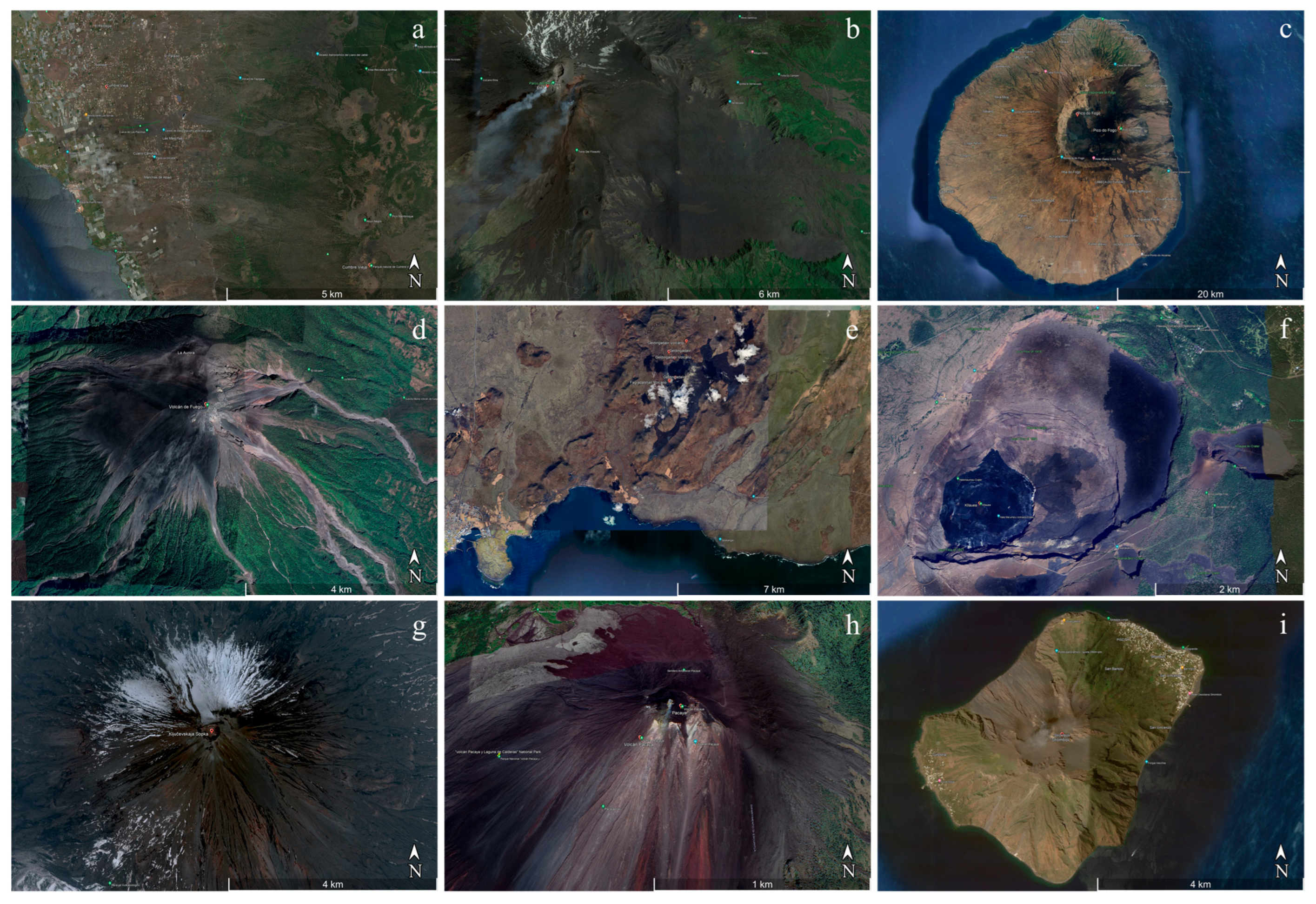
2.1. Volcanoes
2.2. Data Source
3. Method
3.1. Anomalous Volcanic Temperatures
3.2. Theoretical Background
3.3. Three-Step Approach
4. Results
5. Discussion
6. Conclusions
Supplementary Materials
Author Contributions
Funding
Data Availability Statement
Acknowledgments
Conflicts of Interest
References
- Bonaccorso, G. Machine Learning Algorithms; Packt Publishing Ltd.: Birmingham, UK, 2017. [Google Scholar]
- Goodfellow, I.; Bengio, Y.; Courville, A. Deep learning; MIT Press: Cambridge, MA, USA, 2016. [Google Scholar]
- Spinetti, C.; Mazzarini, F.; Casacchia, R.; Colini, L.; Neri, M.; Behncke, B.; Salvatori, R.; Buongiorno, M.F.; Pareschi, M.T. Spectral properties of volcanic materials from hyperspectral field and satellite data compared with LiDAR data at Mt. Etna. Int. J. Appl. Earth Obs. Geoinf. 2009, 11, 142–155. [Google Scholar] [CrossRef]
- Li, L.; Solana, C.; Canters, F.; Chan, J.C.-W.; Kervyn, M. Impact of Environmental Factors on the Spectral Characteristics of Lava Surfaces: Field Spectrometry of Basaltic Lava Flows on Tenerife, Canary Islands, Spain. Remote Sens. 2015, 7, 16986–17012. [Google Scholar] [CrossRef] [Green Version]
- Corradino, C.; Ganci, G.; Cappello, A.; Bilotta, G.; Hérault, A.; Del Negro, C. Mapping Recent Lava Flows at Mount Etna Using Multispectral Sentinel-2 Images and Machine Learning Techniques. Remote Sens. 2019, 11, 1916. [Google Scholar] [CrossRef] [Green Version]
- Amato, E.; Corradino, C.; Torrisi, F.; Del Negro, C. Spectral analysis of lava flows: Temporal and physicochemical effects. Il Nuovo Cimento C 2023. [Accepted for publication]. [Google Scholar]
- Del Negro, C.; Amato, E.; Torrisi, F.; Corradino, C.; Bucolo, M.; Fortuna, L. Support Vector Machine for volcano hazard monitoring from space at Mount Etna. In Proceedings of the 2022 IEEE 21st Mediterranean Electrotechnical Conference (MELECON), Palermo, Italy, 14–16 June 2022; pp. 627–631. [Google Scholar] [CrossRef]
- Amato, E.; Corradino, C.; Torrisi, F.; Del Negro, C. Mapping lava flows at Etna Volcano using Google Earth Engine, open-access satellite data, and machine learning. In Proceedings of the 2021 International Conference on Electrical, Computer, Communications and Mechatronics Engineering (ICECCME), Mauritius, Mauritius, 7–8 October 2021; pp. 1–6. [Google Scholar] [CrossRef]
- Corradino, C.; Bilotta, G.; Cappello, A.; Fortuna, L.; Del Negro, C. Combining Radar and Optical Satellite Imagery with Machine Learning to Map Lava Flows at Mount Etna and Fogo Island. Energies 2021, 14, 197. [Google Scholar] [CrossRef]
- Corradino, C.; Amato, E.; Torrisi, F.; Calvari, S.; Del Negro, C. Classifying Major Explosions and Paroxysms at Stromboli Volcano (Italy) from Space. Remote Sens. 2021, 13, 4080. [Google Scholar] [CrossRef]
- Corradino, C.; Amato, E.; Torrisi, F.; Negro, C.D. Towards an automatic generalized machine learning approach to map lava flows. In Proceedings of the 2021 17th International Workshop on Cellular Nanoscale Networks and their Applications (CNNA), Catania, Italy, 29 September–1 October 2021; pp. 1–4. [Google Scholar] [CrossRef]
- Amato, E. Machine learning and best fit approach to map lava flows from space. Il Nuovo Cimento C 2022, 45, 1–12. [Google Scholar] [CrossRef]
- Torrisi, F. Automatic detection of volcanic ash clouds using MSG-SEVIRI satellite data and machine learning techniques. Il Nuovo Cimento C 2022, 45, 1–10. [Google Scholar] [CrossRef]
- Torrisi, F.; Amato, E.; Corradino, C.; Mangiagli, S.; Del Negro, C. Characterization of Volcanic Cloud Components Using Machine Learning Techniques and SEVIRI Infrared Images. Sensors 2022, 22, 7712. [Google Scholar] [CrossRef]
- Torrisi, F.; Amato, E.; Corradino, C.; Del Negro, C. The FastVRP automatic platform for the thermal monitoring of volcanic activity using VIIRS and SLSTR sensors: FastFRP to monitor volcanic radiative power. Ann. Geophys. 2023, 65, 1. [Google Scholar] [CrossRef]
- Torrisi, F.; Cariello, S.; Corradino, C.; Del Negro, C. Deep learning techniques for monitoring volcanic ash clouds from space. In Proceedings of the 28th IUGG General Assembly, Berlin, Germany, 12–19 July 2023. [Google Scholar]
- Corradino, C.; Ramsey, M.S.; Pailot-Bonnetat, S.; Harris, A.J.L.; Negro, C.D. Detection of Subtle Thermal Anomalies: Deep Learning Applied to the ASTER Global Volcano Dataset. IEEE Trans. Geosci. Remote Sens. 2023, 61, 5000715. [Google Scholar] [CrossRef]
- Han, Z.; Wei, B.; Zheng, Y.; Yin, Y.; Li, K.; Li, S. Breast Cancer Multi-classification from Histopathological Images with Structured Deep Learning Model. Sci. Rep. 2017, 7, 4172. [Google Scholar] [CrossRef] [PubMed]
- Hassan, A.; Mahmood, A. Convolutional Recurrent Deep Learning Model for Sentence Classification. IEEE Access 2018, 6, 13949–13957. [Google Scholar] [CrossRef]
- Yu, Y.; Li, J.; Li, J.; Xia, Y.; Ding, Z.; Samali, B. Automated damage diagnosis of concrete jack arch beam using optimized deep stacked autoencoders and multi-sensor fusion. Dev. Built Environ. 2023, 14, 100128. [Google Scholar] [CrossRef]
- Yu, Y.; Samali, B.; Rashidi, M.; Mohammadi, M.; Nguyen, T.N.; Zhang, G. Vision-based concrete crack detection using a hybrid framework considering noise effect. J. Build. Eng. 2022, 61, 105246. [Google Scholar] [CrossRef]
- Bouindour, S.; Hittawe, M.M.; Mahfouz, S.; Snoussi, H. Abnormal Event Detection Using Convolutional Neural Networks and 1-Class SVM classifier. In Proceedings of the 8th International Conference on Imaging for Crime Detection and Prevention (ICDP 2017), Madrid, Spain, 13–15 December 2017; pp. 1–6. [Google Scholar] [CrossRef]
- Bouindour, S.; Snoussi, H.; Hittawe, M.M.; Tazi, N.; Wang, T. An On-Line and Adaptive Method for Detecting Abnormal Events in Videos Using Spatio-Temporal ConvNet. Appl. Sci. 2019, 9, 757. [Google Scholar] [CrossRef] [Green Version]
- Harrou, F.; Hittawe, M.M.; Sun, Y.; Beya, O. Malicious attacks detection in crowded areas using deep learning-based approach. IEEE Instrum. Meas. Mag. 2020, 23, 57–62. [Google Scholar] [CrossRef]
- Anantrasirichai, N.; Biggs, J.; Albino, F.; Bull, D. A deep learning approach to detecting volcano deformation from satellite imagery using synthetic datasets. Remote Sens. Environ. 2019, 230, 111179. [Google Scholar] [CrossRef] [Green Version]
- LeCun, Y.; Boser, B.; Denker, J.S.; Henderson, D.; Howard, R.E.; Hubbard, W.; Jackel, L.D. Backpropagation Applied to Handwritten Zip Code Recognition. Neural Comput. 1989, 1, 541–551. [Google Scholar] [CrossRef]
- Krizhevsky, A.; Sutskever, I.; Hinton, G.E. ImageNet classification with deep convolutional neural networks. Commun. ACM 2017, 60, 84–90. [Google Scholar] [CrossRef] [Green Version]
- Zisserman, K.S.E.A. Very Deep Convolutional Networks for Large-Scale Image Recognition. arXiv 2014. [Google Scholar] [CrossRef]
- Szegedy, C.; Liu, W.; Jia, Y.; Sermanet, P.; Reed, S.; Anguelov, D.; Erhan, D.; Vanhoucke, V.; Rabinovich, A. Going Deeper With Convolutions. In Proceedings of the IEEE Conference on Computer Vision and Pattern Recognition (CVPR), Boston, MA, USA, 7–12 June 2015. [Google Scholar]
- He, K.; Zhang, X.; Ren, S.; Sun, J. Deep Residual Learning for Image Recognition. In Proceedings of the 2016 IEEE Conference on Computer Vision and Pattern Recognition (CVPR), Las Vegas, NV, USA, 27–30 June 2016; pp. 770–778. [Google Scholar] [CrossRef] [Green Version]
- Iandola, F.N.; Han, S.; Moskewicz, M.W.; Ashraf, K.; Dally, W.J.; Keutzer, K. SqueezeNet: AlexNet-level accuracy with 50x fewer parameters and <0.5MB model size 2016. arXiv 2016, arXiv:1602.07360. [Google Scholar]
- Deng, J.; Dong, W.; Socher, R.; Li, L.-J.; Li, K.; Fei-Fei, L. ImageNet: A large-scale hierarchical image database. In Proceedings of the 2009 IEEE Conference on Computer Vision and Pattern Recognition, Miami, FL, USA, 20–25 June 2009; pp. 248–255. [Google Scholar] [CrossRef] [Green Version]
- Huang, J.; Lu, X.; Chen, L.; Sun, H.; Wang, S.; Fang, G. Accurate Identification of Pine Wood Nematode Disease with a Deep Convolution Neural Network. Remote Sens. 2022, 14, 913. [Google Scholar] [CrossRef]
- Gaddes, M.E.; Hooper, A.; Bagnardi, M. Using Machine Learning to Automatically Detect Volcanic Unrest in a Time Series of Interferograms. J. Geophys. Res. Solid Earth 2019, 124, 12304–12322. [Google Scholar] [CrossRef] [Green Version]
- Kato, S.; Miyamoto, H.; Amici, S.; Oda, A.; Matsushita, H.; Nakamura, R. Automated classification of heat sources detected using SWIR remote sensing. Int. J. Appl. Earth Obs. Geoinf. 2021, 103, 102491. [Google Scholar] [CrossRef]
- Yang, Q.; Zhang, Y.; Dai, W.; Pan, S.J. Transfer Learning; Cambridge University Press: Cambridge, UK, 2020. [Google Scholar]
- Yin, X.; Chen, W.; Wu, X.; Yue, H. Fine-tuning and visualization of convolutional neural networks. In Proceedings of the 2017 12th IEEE Conference on Industrial Electronics and Applications (ICIEA), Siem Reap, Cambodia, 18–20 June 2017; pp. 1310–1315. [Google Scholar] [CrossRef]
- Weidman, S. Deep Learning from Scratch: Building with Python from First Principles; O’Reilly Media: Newton, MA, USA, 2019. [Google Scholar]
- Gorelick, N.; Hancher, M.; Dixon, M.; Ilyushchenko, S.; Thau, D.; Moore, R. Google Earth Engine: Planetary-scale geospatial analysis for everyone. Remote Sens. Environ. 2017, 202, 18–27. [Google Scholar] [CrossRef]
- Carneiro, T.; Da Nobrega, R.V.M.; Nepomuceno, T.; Bian, G.-B.; De Albuquerque, V.H.C.; Filho, P.P.R. Performance Analysis of Google Colaboratory as a Tool for Accelerating Deep Learning Applications. IEEE Access 2018, 6, 61677–61685. [Google Scholar] [CrossRef]
- Rabuffi, F.; Silvestri, M.; Musacchio, M.; Romaniello, V.; Buongiorno, M.F. A Statistical Approach to Satellite Time Series Analysis to Detect Changes in Thermal Activities: The Vulcano Island 2021 Crisis. Remote Sens. 2022, 14, 3933. [Google Scholar] [CrossRef]
- Wright, R.; Blake, S.; Harris, A.J.L.; Rothery, D.A. A simple explanation for the space-based calculation of lava eruption rates. Earth Planet. Sci. Lett. 2001, 192, 223–233. [Google Scholar] [CrossRef]
- Harris, A.J.L.; Dehn, J.; Calvari, S. Lava effusion rate definition and measurement: A review. Bull. Volcanol. 2007, 70, 1–22. [Google Scholar] [CrossRef]
- Harris, A.J.L.; Baloga, S.M. Lava discharge rates from satellite-measured heat flux. Geophys. Res. Lett. 2009, 36, L19302. [Google Scholar] [CrossRef]
- Ganci, G.; Cappello, A.; Bilotta, G.; Hérault, A.; Zago, V.; Del Negro, C. Mapping Volcanic Deposits of the 2011–2015 Etna Eruptive Events Using Satellite Remote Sensing. Front. Earth Sci. 2018, 6, 83. [Google Scholar] [CrossRef]
- Patrick, M.R.; Kauahikaua, J.; Orr, T.; Davies, A.; Ramsey, M. Operational thermal remote sensing and lava flow monitoring at the Hawaiian Volcano Observatory. In Detecting, Modelling and Responding to Effusive Eruptions; Harris, A.J.L., De Groeve, T., Garel, F., Carn, S.A., Eds.; Geological Society of London: London, UK, 2016; Volume 426, pp. 489–503. [Google Scholar]
- Wright, R.; Flynn, L.P.; Garbeil, H.; Harris, A.J.L.; Pilger, E. MODVOLC: Near-real-time thermal monitoring of global volcanism. J. Volcanol. Geotherm. Res. 2004, 135, 29–49. [Google Scholar] [CrossRef]
- Harris, A. Thermal Remote Sensing of Active Volcanoes: A User’s Manual; Cambridge University Press: Cambridge, UK, 2013. [Google Scholar]
- Thompson, J.O.; Ramsey, M.S. The influence of variable emissivity on lava flow propagation modeling. Bull. Volcanol 2021, 83, 41. [Google Scholar] [CrossRef]
- Oppenheimer, C.; Yirgu, G. Thermal imaging of an active lava lake: Erta ’Ale volcano, Ethiopia. Int. J. Remote Sens. 2002, 23, 4777–4782. [Google Scholar] [CrossRef]
- Fink, J.H. Lava Flows and Domes, Emplacement, Mechanisms and Hazard Implications. In Wooster and Rothery 1990; Springer: Berlin/Heidelberg, Germany, 1990. [Google Scholar]
- Hazlett, R.W. Geology of the San Cristobal volcanic complex, Nicaragua. J. Volcanol. Geotherm. Res. 1987, 33, 223–230. [Google Scholar] [CrossRef]
- Shinohara, H.; Giggenbach, W.F.; Kazahaya, K.; Hedenquist, J.W. Geochemistry of volcanic gases and hot springs of Satsuma-Iwojima, Japan: Following Matsuo. Geochem. J. 1993, 27, 271–285. [Google Scholar] [CrossRef]
- Paszke, A.; Gross, S.; Massa, F.; Lerer, A.; Bradbury, J.; Chanan, G.; Killeen, T.; Lin, Z.; Gimelshein, N.; Antiga, L.; et al. Pytorch: An imperative style, high-performance deep learning library. Adv. Neural Inf. Process. Syst. 2019, 32. [Google Scholar]
- Lin, W.; Wu, Z.; Lin, L.; Wen, A.; Li, J. An Ensemble Random Forest Algorithm for Insurance Big Data Analysis. IEEE Access 2017, 5, 16568–16575. [Google Scholar] [CrossRef]
- James, G.; Witten, D.; Hastie, T.; Tibshirani, R. An Introduction to Statistical Learning; Springer: New York, NY, USA, 2013. [Google Scholar]
- Steffke, A.M.; Harris, A.J.L. A review of algorithms for detecting volcanic hot spots in satellite infrared data. Bull. Volcanol. 2011, 73, 1109–1137. [Google Scholar] [CrossRef]
- Genzano, N.; Pergola, N.; Marchese, F. A Google Earth Engine Tool to Investigate, Map and Monitor Volcanic Thermal Anomalies at Global Scale by Means of Mid-High Spatial Resolution Satellite Data. Remote Sens. 2020, 12, 3232. [Google Scholar] [CrossRef]
- Coppola, D.; Laiolo, M.; Cigolini, C.; Donne, D.D.; Ripepe, M. Enhanced volcanic hot-spot detection using MODIS IR data: Results from the MIROVA system. Geol. Soc. Lond. Spéc. Publ. 2016, 426, 181–205. [Google Scholar] [CrossRef]
- Corradino, C.; Amato, E.; Torrisi, F.; Del Negro, C. Data-Driven Random Forest Models for Detecting Volcanic Hot Spots in Sentinel-2 MSI Images. Remote Sens. 2022, 14, 4370. [Google Scholar] [CrossRef]
- Lin, Z.; Ji, K.; Leng, X.; Kuang, G. Squeeze and Excitation Rank Faster R-CNN for Ship Detection in SAR Images. IEEE Geosci. Remote Sens. Lett. 2019, 16, 751–755. [Google Scholar] [CrossRef]
- Carranza-García, M.; García-Gutiérrez, J.; Riquelme, J.C. A Framework for Evaluating Land Use and Land Cover Classification Using Convolutional Neural Networks. Remote Sens. 2019, 11, 274. [Google Scholar] [CrossRef] [Green Version]
- Zhang, C.; Sargent, I.; Pan, X.; Li, H.; Gardiner, A.; Hare, J.; Atkinson, P.M. Joint Deep Learning for land cover and land use classification. Remote Sens. Environ. 2019, 221, 173–187. [Google Scholar] [CrossRef] [Green Version]
- Li, J.; Roy, D.P. A Global Analysis of Sentinel-2A, Sentinel-2B and Landsat-8 Data Revisit Intervals and Implications for Terrestrial Monitoring. Remote Sens. 2017, 9, 902. [Google Scholar] [CrossRef] [Green Version]


| Volcano | Eruptive Activity between 2013 and 2022 |
|---|---|
| Cumbre Vieja | 2021 |
| Etna | 2013–2014–2017–2018–2019–2020–2021–2022 |
| Pico do Fogo | 2014–2015 |
| Volcán de Fuego | 2017–2019–2020–2021 |
| Geldingadalir | 2020–2021 |
| Kīlauea | 2020–2021 |
| Klyuchevskaya | 2020–2021 |
| Pacaya | 2020–2021 |
| Stromboli | 2014–2019–2020–2021 |
| Date (dd/mm/yyyy) | Satellite | Volcano | Activity (Yes: 1, No: 0) | Date (dd/mm/yyyy) | Satellite | Volcano | Activity (Yes: 1, No: 0) |
|---|---|---|---|---|---|---|---|
| 03/05/2013 | Landsat 8 | Etna | 0 | 03/02/2021 | Sentinel-2 | Geldingadalir | 0 |
| 19/05/2013 | Landsat 8 | Etna | 0 | 07/02/2021 | Sentinel-2 | Cumbre Vieja | 0 |
| 02/09/2014 | Landsat 8 | Etna | 0 | 18/02/2021 | Sentinel-2 | Etna | 1 |
| 19/09/2014 | Landsat 8 | Stromboli | 1 | 21/02/2021 | Sentinel-2 | Etna | 1 |
| 28/02/2015 | Landsat 8 | Fogo | 0 | 25/02/2021 | Landsat 8 | Fuego | 0 |
| 07/10/2015 | Landsat 8 | Etna | 0 | 25/02/2021 | Landsat 8 | Pacaya | 1 |
| 03/12/2015 | Landsat 8 | Etna | 1 | 06/03/2021 | Landsat 8 | Geldingadalir | 0 |
| 16/03/2017 | Sentinel-2 | Etna | 1 | 13/03/2021 | Landsat 8 | Geldingadalir | 0 |
| 18/05/2017 | Sentinel-2 | Etna | 0 | 22/03/2021 | Landsat 8 | Geldingadalir | 1 |
| 24/03/2018 | Sentinel-2 | Etna | 0 | 25/03/2021 | Sentinel-2 | Pacaya | 1 |
| 08/05/2018 | Sentinel-2 | Etna | 0 | 04/05/2021 | Sentinel-2 | Geldingadalir | 1 |
| 10/05/2018 | Sentinel-2 | Etna | 0 | 17/05/2021 | Sentinel-2 | Etna | 0 |
| 30/05/2018 | Sentinel-2 | Etna | 0 | 19/05/2021 | Sentinel-2 | Pacaya | 0 |
| 29/06/2018 | Sentinel-2 | Etna | 0 | 19/05/2021 | Sentinel-2 | Etna | 1 |
| 24/12/2018 | Sentinel-2 | Etna | 1 | 25/05/2021 | Landsat 8 | Etna | 1 |
| 14/06/2019 | Sentinel-2 | Etna | 0 | 27/05/2021 | Sentinel-2 | Kīlauea | 0 |
| 19/07/2019 | Sentinel-2 | Etna | 1 | 13/06/2021 | Sentinel-2 | Etna | 1 |
| 27/07/2019 | Sentinel-2 | Etna | 1 | 16/06/2021 | Sentinel-2 | Kīlauea | 0 |
| 18/08/2019 | Sentinel-2 | Etna | 0 | 12/08/2021 | Sentinel-2 | Geldingadalir | 1 |
| 02/04/2020 | Sentinel-2 | Klyuchevskaya | 0 | 12/08/2021 | Sentinel-2 | Geldingadalir | 1 |
| 04/04/2020 | Sentinel-2 | Klyuchevskaya | 0 | 20/08/2021 | Sentinel-2 | Stromboli | 0 |
| 11/06/2020 | Sentinel-2 | Kīlauea | 0 | 26/08/2021 | Sentinel-2 | Cumbre Vieja | 0 |
| 23/07/2020 | Sentinel-2 | Pacaya | 0 | 30/08/2021 | Sentinel-2 | Etna | 1 |
| 16/09/2020 | Sentinel-2 | Klyuchevskaya | 0 | 09/09/2021 | Sentinel-2 | Stromboli | 0 |
| 20/10/2020 | Landsat 8 | Fuego | 0 | 21/09/2021 | Landsat 8 | Etna | 1 |
| 10/11/2020 | Sentinel-2 | Klyuchevskaya | 1 | 21/09/2021 | Sentinel-2 | Stromboli | 0 |
| 21/11/2020 | Landsat 8 | Geldingadalir | 0 | 03/11/2021 | Sentinel-2 | Etna | 0 |
| 28/12/2020 | Sentinel-2 | Kīlauea | 1 | 05/11/2021 | Sentinel-2 | Etna | 0 |
| 18/01/2021 | Sentinel-2 | Etna | 1 | 28/11/2021 | Sentinel-2 | Kīlauea | 1 |
| 24/01/2021 | Landsat 8 | Geldingadalir | 0 | 08/02/2022 | Sentinel-2 | Etna | 0 |
Disclaimer/Publisher’s Note: The statements, opinions and data contained in all publications are solely those of the individual author(s) and contributor(s) and not of MDPI and/or the editor(s). MDPI and/or the editor(s) disclaim responsibility for any injury to people or property resulting from any ideas, methods, instructions or products referred to in the content. |
© 2023 by the authors. Licensee MDPI, Basel, Switzerland. This article is an open access article distributed under the terms and conditions of the Creative Commons Attribution (CC BY) license (https://creativecommons.org/licenses/by/4.0/).
Share and Cite
Amato, E.; Corradino, C.; Torrisi, F.; Del Negro, C. A Deep Convolutional Neural Network for Detecting Volcanic Thermal Anomalies from Satellite Images. Remote Sens. 2023, 15, 3718. https://doi.org/10.3390/rs15153718
Amato E, Corradino C, Torrisi F, Del Negro C. A Deep Convolutional Neural Network for Detecting Volcanic Thermal Anomalies from Satellite Images. Remote Sensing. 2023; 15(15):3718. https://doi.org/10.3390/rs15153718
Chicago/Turabian StyleAmato, Eleonora, Claudia Corradino, Federica Torrisi, and Ciro Del Negro. 2023. "A Deep Convolutional Neural Network for Detecting Volcanic Thermal Anomalies from Satellite Images" Remote Sensing 15, no. 15: 3718. https://doi.org/10.3390/rs15153718