Article

Mapping Irish Water Bodies: Comparison of Platforms, Indices and Water Body Type

by
Minyan Zhao
1 and
Fiachra O’Loughlin
1,2,*
1
Dooge Centre for Water Resources Research, School of Civil Engineering, University College Dublin, D04 V1W8 Dublin, Ireland
2
UCD Earth Institute, University College Dublin, D04 V1W8 Dublin, Ireland
*
Author to whom correspondence should be addressed.
Remote Sens. 2023, 15(14), 3677; https://doi.org/10.3390/rs15143677
Submission received: 31 May 2023 / Revised: 20 July 2023 / Accepted: 21 July 2023 / Published: 23 July 2023

Abstract

:
Accurate monitoring of water bodies is essential for the management and regulation of water resources. Traditional methods for measuring water quality are always time-consuming and expensive; furthermore, it can be very difficult capture the full spatiotemporal variations across regions. Many studies have shown the possibility of remote-sensing-based water monitoring work in many areas, especially for water quality monitoring. However, the use of optical remotely sensed imagery depends on several factors, including weather, quality of images and the size of water bodies. Hence, in this study, the feasibility of optical remote sensing for water quality monitoring in the Republic of Ireland was investigated. To assess the value of remote sensing for water quality monitoring, it is critical to know how well water bodies and the existing in situ monitoring stations are mapped. In this study, two satellite platforms (Sentinel-2 MSI and Landsat-8 OLI) and four indices for separating water and land pixel (Normalized Difference Vegetation Index—NDVI; Normalized Difference Water Index—NDWI; Modified Normalized Difference Water Index—MNDWI; and Automated Water Extraction Index—AWEI) have been used to create water masks for two scenarios. In the first scenario (Scenario 1), we included all pixels classified as water, while for the second scenario (Scenario 2) accounts for potential land contamination and only used water pixels that were completed surround by other water pixels. The water masks for the different scenarios and combinations of platforms and indices were then compared with the existing water quality monitoring station and to the shapefile of the river network, lakes and coastal and transitional water bodies. We found that both platforms had potential for water quality monitoring in the Republic of Ireland, with Sentinel-2 outperforming Landsat due to its finer spatial resolution. Overall, Sentinel-2 was able to map ~25% of the existing monitoring station, while Landsat-8 could only map ~21%. These percentages were heavily impacted by the large number of river monitoring stations that were difficult to map with either satellite due to their location on smaller rivers. Our results showed the importance of testing several indices. No index performed the best across the different platforms. AWEInsh (Automated Water Extraction Index—no shadow) and Sentinel-2 outperformed all other combinations and was able to map over 80% of the area of all non-river water bodies across the Republic of Ireland. While MNDWI was the best index for Landsat-8, it was the worst performer for Sentinel-2. This study showed that optical remote sensing has potential for water monitoring in the Republic of Ireland, especially for larger rivers, lakes and transitional and coastal water bodies.

Graphical Abstract

1. Introduction

It is critical that we sustain and improve our water resources as they are inseparable from the ecosystems and are necessary for life [1]. The pressures on water resources are increasing globally with ever-growing demands for freshwater, over-abstraction of water resources, pollution and climate change [2]. One of the most effective controls to prevent water pollution is to identify the potential sources promptly [3]; therefore, it is crucial to obtain timely access to water information, such as water quality and water quantity.
Under the European Union’s Water Framework Directive (WFD), which came into force in 2000 [4], and the National Hydrometric Monitoring Program [5], information on water quality and quantity across Ireland is collected periodically via conventional methods [6]; for example, water flow in some locations is measured via the use of weirs or handheld mechanical current meter, while water quality parameters are derived from laboratory analyses undertaken on water samples collected at each monitoring station. This approach provides precise information on water at discrete sampling points; however, it cannot grasp the spatiotemporal aspects of water quality that occur in large water bodies [7]. Across the Republic of Ireland, there are 4829 water bodies designated by the WFD; however, only approximately two-thirds of these are included in the national WFD monitoring program, and this does not include all water bodies. This can be broken down to its constituent parts, with 74% of river bodies, 6.8% of lakes and 40% of coastal and transitional waters currently monitored [6].
Remote sensing (RS), with its frequent revisit time and large spatial coverage, is an alternative approach to facilitating water monitoring [8]. The use of RS in water quality monitoring started in the early 1970s [9], when the correlation between solar radiation reflectance and sediment concentration was investigated [10]. Today, RS is used in many aspects of water resources including flooding estimation, water erosion assessment, water area detection, the phenology of water cycle, water quality derivation, etc. [11]. In Ireland, very few studies have investigated the use of remote sensing for water resources (e.g., [12,13,14]). Agarwal et al. [12] and Karki et al. [13], as part of the Remote Sensing of Irish Surface Waters Project (INFER), used remote sensing to estimate the chlorophyll-a content, turbidity, and algal coverage in some regional Irish transitional and coastal (TraC) areas. However, the feasibility of RS at national scale for water quality monitoring has not been established.
To establish if remote sensing has potential in water quality monitoring in Ireland, it is first necessary to see if the spatial coverage is sufficient. One way to test this is via the generation of water masks, which separate land and water pixels. The spectral, temporal, radiometric and spatial resolutions of different satellite platforms are the determining factors in this. Therefore, the choice of RS platforms is important. For example, MODIS (Moderate Resolution Imaging Spectroradiometer), onboard the Terra and Aqua spacecrafts, has the advantage of high temporal resolution (1–2 times/day), broad spectral range (0.4–14.4 μm) and long tracking history (1999–present) [14]. It has been utilized in tracking surface water evolutions [15,16,17]. However, its disadvantage is its spatial resolution, which ranges from 250 to 1000 m, restricting application only to large areas [14]. The deployment of different high-resolution platforms offers great possibilities in detecting smaller water bodies. IKONOS, one of the first high-spatial resolution satellites, has been used to map lake areas in Myanmar [18]. However, the presence of shadows on IKONOS images makes water detection harder [19]. In recent years, high resolution data are becoming more easily accessible, with more than 1600 CubeSats currently orbiting the Earth’s surfaces. These CubeSat have approximately daily revisit times and their 3-m spatial resolution is much higher than many of the other high-resolution products available [20]. CubeSats have been used to monitor lake dynamics in Arctic-Boreal [21], in Yukon Flats, US [22] and in the Tocantins–Araguaia hydrographic region, Brazil [23]. However, the relatively low radiometric quality and inter-sensors inconsistencies of CubeSats have posed limitations in water monitoring [24]. Two platforms that have been widely used in aquatic science are the Landsat missions and Sentinel-2. These platforms, with their 30- and 20-m resolutions, respectively, are freely available and have the ideal spectral range for aquatic science [25,26]. Some of the uses of Landsat include the generation of global river widths [27]; multi-temporal global water masks [28]; and water masks and river widths in Congo [29] and North America [30]. Sentinel-2, despite being a relatively newer platform has also had a range of applications from coastal shoreline mapping [31] to surface water mapping across France [32] to mapping the tidal flat around the Bohai and Yellow Seas [33]. In some cases, both Landsat and Sentinel-2 have been combined—e.g., Pardo-Pascual et al. [34]—for mapping the shoreline of natural beaches.
To generate water masks from remote sensing, there are various approaches available. Yang et al. [32] has classified these approaches into two groups: (1) sample-based methods; and (2) rule-based methods. Sample-based methods classify the water pixels based on the supervised classification at pixel and object levels within the same groups [35]. The accuracy of this method depends on prior reliable knowledge, which is usually acquired at a high cost. Rule-based approaches, on the other hand, are faster and more convenient to use than sample-based methods and are therefore more widely used. Rule-based methods normally rely on proven algorithms based on comparing the surface reflectance of spectral bands [32]. While there is a large selection of water spectral indices, the Normalized Difference Water index (NDWI) was the first index proposed for water extraction. Though it suffers from noise in build-up areas, which affects accuracy, the Modified Normalized Difference Water Index (MNDWI) was created to address this issue [1]. However, it cannot distinguish between water and snow [36]. To further improve water mapping accuracy, the Automated Water Extraction Index (AWEI) was then created, which includes two indices capable of shadow and non-shadow scenarios, respectively [37]. While the above are the most commonly used water indices, many more have been created to address other shortcomings. For example, the Water Index2015 (WI2015) [38] was developed to improve the performance of classifying water pixels via Landsat. The Water Ratio Index (WRI), High Resolution Water Index (HRWI) and Enhanced Water Index (EWI) were developed for urban areas and cities and have been shown to perform better than other more widely used water indices [39,40,41]. Recently, to improve upon the MNDWI, the Contrast Difference Water Index (CDWI) and the Shadow Difference Water Index (SDWI) were created for built-up and non-built-up areas, respectively, and the BDWI (Background Difference Water Index) was designed for complex background [42]. Other indices, such as the NDVI (Normalized Difference Vegetation Index) and EVI (Enhanced Vegetation Index), which were developed for extracting land pixel areas, have been used in distinguishing water from land [43,44]. Memon et al. [45] compared NDWI with two other indices—Red and Short-Wave Infra-Red (RSWIR) and MNDWI in Pakistan—and showed the tendencies of NDWI to underestimate the inundated area. Acharya, Subedi and Lee [43] compared the same indices for Nepal and found that NDVI and NDWI showed better results than MNDWI and AWEI for pure water pixels. Liu et al. [46] and Du et al. [47] compared various water indices (NDWI, MNDWI, AWEI and WI2015) in Guangzhou and the Venice coastland, respectively, and demonstrated that pan-sharpened WI2015 and MNDWI provide more accurate results than the other indices. The AWEI was compared with both MNDWI and Maximum Likelihood (ML) for Denmark, Switzerland, Ethiopia, South Africa and New Zealand, and the results showed that the accuracy of the AWEI was much higher than the other two indices [37]. Furthermore, Sivanpillai et al. [48] showed that the MNDWI outperformed NDWI in calculating pre- and post-flood inundation extents in the US. In addition to the use of these indices, machine learning methods are also becoming popular for the extraction of water bodies. These machine learning methods include regression trees, neural networks and support vector machines, and several studies have compared these methods [49,50,51].
The overall objective of this study is to help assess the value of remote sensing optical imagery for water quality monitoring of water bodies across the Republic of Ireland. To answer this objective, it is critical to know the extent to which remote sensing can map the different water bodies, and three sub-objectives will be addressed:
  • What percentages of water bodies are mapped by the different remote sensing platforms? What is the difference between using Landsat-8 or Sentinel-2?
  • Which is the best water index for detecting water pixels across Ireland? Does this vary by water body type?
  • How well does remote sensing map the existing in situ monitoring points? This is critical for the calibration of water quality estimates from remote sensing.

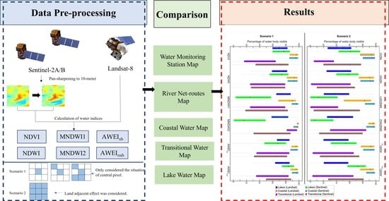
2. Study Area and Methodology

2.1. Study Area

In this study, we focus on the Republic of Ireland, which is in the northwest of Europe (Figure 1). The Republic of Ireland covers five-sixths of Ireland’s surface, with a total area of 70,273 km2, and the remainder is Northern Ireland [52]. The Republic of Ireland has over 12,200 lakes; however, only 812 have been designated as lake water bodies by the WFD [53]. These lake water bodies are predominately small (66% < 1 ha) and mostly in Western Ireland. Furthermore, Ireland has more than 74,000 km of river channels [54], where first- and second-order streams account for 95.8% of the total (https://gis.epa.ie/, accessed on 22 July 2023).
Water quality is monitored in the Republic of Ireland by the Irish Environmental Agency (EPA) [55] to ensure that it adheres to European legislation such as the WFD and directives pertaining to nitrates, habitats, groundwater, drinking water and bathing water [56]. The Republic of Ireland is currently in the third cycle (2022–2027) of the WFD directive [57]. However, at the end of the second WFD cycle, the EPA reported that while almost half of Ireland’s rivers and lakes (50% and 69%, respectively) meet or exceed the mandatory ‘good ecological status’, 64% of estuaries failed to meet the WFD’s mandatory ‘good ecological status’ standard (https://www.epa.ie/publications/monitoring--assessment/freshwater--marine/).
Under the third WFD cycle, the EPA has broken down the Republic of Ireland into 46 catchments and 583 sub-catchment units for reporting purposes. There are a total of 4842 water bodies, with 3–15 water bodies in each sub-catchment [58]. The total area of transitional, coastal and lake water bodies monitored in this cycle are 842.37 km2, 13,642.07 km2 and 1200.31 km2, respectively. The total number of monitoring points is 14,097, with 13,706 of them monitoring surface water bodies. The physical, chemical and biological changes in each water body are monitored with the sampling frequency depending on parameter and water types. For example, chemical oxygen demand (COD) is sampled an average of 80 times per month nationally, while the sampling time for nitrogen is 229 times per month nationally.

2.2. Earth Observation Platforms

Two satellites missions with publicly available data—Sentinel-2A/B multi-spectral instrument (MSI) and Landsat-8 Operational Land Imager (OLI)—were used in this study. Sentinel-2A/B are two identical Earth Observation satellites launched in June 2015 and March 2017 by the European Space Agency as part of the Copernicus Project (GMES). These satellites have spectral bands that span from the visible (VIS) to the short wave infrared (SWIR) (458–2280 nm) at high spatial resolution (10 m to 60 m), with a revisit time of 5 days at the equator [59].
Landsat-8 was launched by the U.S. Geological Survey (USGS) in February 2013 and carries a two-sensor payload (Operational Land Imager (OLI) and the Thermal Infrared Sensor (TIRS)) with a revisit time of 16 days [60]. Landsat-8 OLI was used, and it has a spectral range of Landsat-8 OLI (435–2294 nm) with a spatial resolution of 30 m. Detailed band information of each platform is listed in Table 1.

2.3. Methodology

The method used in this research is depicted in Figure 2. In the following sections, the different stages of the research will be explained as follows: (a) two datasets have been pre-processed in the Google Earth Engine (GEE); the pre-process includes image selection, band selection and the creation of image catalogs; (b) to fit different resolutions of Sentinel-2, pan-sharpening was used in upscaling the 20-m band of Sentinel-2 to 10-m; (c) the calculation of the water indices: NDVI, NDWI, MNDWI and AWEI; and (d) the comparison of the maps from satellites with EPA datasets.

2.3.1. Pre-Processing

Sentinel-2A/B MSI and Landsat-8 OLI, from January 2018 to December 2019, were initially processed on the Google Earth Engine (GEE) platform (https://code.earthengine.google.com/). GEE is a cloud-based geospatial analysis platform used for geographical computing and analysis, which allows academic users free access to the process and to analyze large amounts of data as they need [61], and the time period was chosen to ensure that a cloud free mosaic was able to be produce across the entire Republic of Ireland.
The Sentinel-2A/B level 2A and Landsat-8 Tier 1 datasets were used in this study. Level 2A is bottom-of-atmosphere (BOA) dataset, which are produced from level-1C data (top of atmosphere) via Sen2Cor [62], while Landsat-8 Collection 2 Tier 1 is the highest quality radiometric and positional data available.
The first step in pre-processing was to select images with cloud coverage less than 20%; then, cloud pixels were removed from Sentinel-2A/B and Landsat-8 imagery using the QA60 band and CFMask, respectively. The QA60 band is a bitmask band which contains cloud mask information, while CFMask is the C implementation of function of Mask, initially created by Zhu [63]. It is currently utilized by USGS to identify clouds, cloud shadows, cirrus, snow and ice during OLI data processing [64]. Its accuracy has been tested and compared with the other cloud detection algorithms (See5, Automated Cloud Cover Assessment (ACCA), Artificial Thermal-Automated Cloud Cover Algorithm (AT-ACCA), Fixed Temperature-Automated Cloud Cover Algorithm (FT-ACCA)) [65]. Results showed that CFMask outperforms other methods, producing the highest accuracy for cloud shadow results and working without geographic restrictions. While CFMask is a spectral characteristic-based multi-pass algorithm which used decision trees to produce two potential cloud masks, cloud mask was produced by combining these two potential cloud masks together [63].

2.3.2. Panchromatic Sharpening

An additional processing step was required for Sentinel-2 data to ensure that the spatial resolution of all bands in generating water masks are identical. Sentinel’s SWIR1 and SWIR2 (Table 1) bands have a spatial resolution of 20 m, while Bands 2, 3, 4 and 8 are all at 10 m. Therefore, to obtain more explicit spatial information from Sentinel-2, panchromatic sharpening or pan-sharpening was necessary to upscale SWIR1 and SWIR2, and the overview of the process is shown in Figure 3.
Band 11 and Band 12 have first been resampled to 10 m via nearest neighbor interpolation because nearest neighbor interpolation reserves the properties of the original dataset and is highly efficient compared to other resampling techniques over large areas. Additionally, previous research has shown that the selection of different resampling methods will not have a significant effect on the final visual appearance of fused images. Pan-sharpening is a technique that combines high-resolution detail from a panchromatic band with the lower-resolution color information of coarse bands, and it can help obtain a higher resolution map, which is crucial in some studies [66]. First, the lower resolution bands were needed to resample to obtain the same resolution with high-resolution band [67]. Many pan-sharpening approaches have been used and compared in extracting water masks [68,69]. One of the most common methods is the High Pass Filter (HPF) [70]. The HPF uses a filter to add information from the high-resolution image to the low-resolution image. This filter has a specified weight, and there are many kinds of soothing filters, including the Box (used in this study), Gaussian, and Laplacian. Du et al. [47] tested different image pan-sharpening approaches to generate the water masks at the Venice coastland, Italy, and showed that HPF was the most accurate method.

2.3.3. Water Mask Creation

The water indices from Landsat-8 were created directly on GEE, while Matlab2022a was used for Sentinel-2 to overcome the computation limit of GEE and the need for pan-sharpening Sentinel-2 images prior to water mask creation. For both Landsat-8 and Sentinel-2, water masks were created for four different indices: NDVI, NDWI, MNDWI and AWEI ((1)–(6)).
NDVI = NIR     Red NIR   +   Red
NDWI = Green     NIR Green   +   NIR
MNDWI 1 = Green     SWIR 1 Green   +   SWIR 1
MNDWI 2 = Green     SWIR 1 Green   +   SWIR 2  
AWEI sh = Blue + 2.5 × Green 1.5 × ( NIR + SWIR 1 ) 0.25 × SWIR 2
AWEI nsh = 4 × ( Green SWIR 1 ) ( 0.25 × NIR + 2.75 × SWIR 2 ) .
For each of these indices’, binary maps, where 1 is water and 0 is land, were produced using the Bottom Valley threshold approach. This approach locates the lowest point between the two peaks, which is deemed the threshold for separating water and land pixels. The Otsu threshold approach [71] was also tested; however, this method resulted in the incorrect classification of pixels as land or water. Previous studies have noted this same issue with Ostu when the amplitudes of the bimodal are largely different, which causes the Ostu threshold to become biased [69,72]. Figure 4 shows the different thresholds calculated using the Otsu and the Bottom Valley approaches and shows the bias in the Ostu threshold.

2.3.4. Comparison of Binary Water Masks

Two sets of binary maps were created for two different scenarios. Scenario 1 ignores many potential sources of errors, including boundary effects such as land contamination at the edge of water pixels [73], and assumes that if a pixel is classified as water, it is water. However, Scenario 2 aims to account for these boundary effects by only classifying a pixel as water if it classified as a water pixel itself and is also surrounded by other classified water pixels. This approach was previously applied to remove the boundary effect on ICESat [74].
Scenario 1 and Scenario 2 for the detection of water were compared with datasets available from the Irish EPA to investigate the spatial coverage of water bodies by the two remote sensing platforms and the impact of using different indices in distinguishing water land pixels. Comparison datasets include national water monitoring stations, shapefile of river net-routes, lake, coastal and transitional water bodies, and all were downloaded from the EPA website (https://gis.epa.ie/EPAMaps/). These datasets are for third-cycle WFD and are shown in Figure 2 gray frame.
The national water monitoring station map includes all 9736 rivers, 2883 lakes, 603 transitional, 484 coastal and 391 groundwater monitoring stations (although the groundwater stations were not applicable to this study). These monitoring stations are used for the WFD to periodically monitor water quality (e.g., concentration of chlorophyll-a and phosphorus). Therefore, it is important that remote sensing imagery is able to map these locations so that relationships between in situ measurements and remotely sensed optical properties can be developed. The river shapefile comprises over 100,000 polylines with the stream order information. The lakes, transitional and coastal maps comprise 810, 108 and 194 polygons, respectively. Since this study focused on the Republic of Ireland, the water bodies which lie entirely in Northern Ireland have been removed manually.
The binary maps for each scenario and for every index used for each platform were compared with the EPA data, and the following percentages were calculated:
  • Percentage of water cells which overlay water monitoring stations;
  • The percentage of lakes mapped and their areas;
  • The percentage of rivers mapped and their stream order;
  • Percentage of coastal and transitional areas mapped.

3. Results

3.1. Water Masks

Two regions in the Republic of Ireland were chosen to show the detailed results of the impact of using the different platforms and indices (Figure 5). The first region, as shown in Figure 5b, is Lough Derg. Lough Derg is the third-largest lake in the Republic of Ireland and is in the Lower Shannon River basin. This area is predominately rural. The second region is centered around Dublin City and Bay (Figure 5c). Dublin is the capital city of the Republic of Ireland, is heavily urbanized and is located on the east coast of Ireland.
The water masks of Lough Derg and Dublin Bay mapped via Landsat-8 are depicted in Figure 6, corresponding to Scenario 1 and Scenario 2, while Figure 7 depicts those derived from Sentinel-2. The shape of Lough Derg was clearly mapped by all indices and platforms and for both scenarios, as was the river meander just south of Lough Derg, except for MNDWI2 via Sentinel-2. Although Sentinel-2 did map more details due to its higher spatial resolution, as expected, more of the river network was mapped in the Sentinel-2 water masks compared with those derived from Landsat. However, all indices did not perform equally across the platforms. By comparing Figure 6 and Figure 7, it is clear that for Landsat, MNDWI1 was able to map more of the river network compared with the other indices, while for Sentinel-2, AWEIsh outperformed the other indices. The results for Dublin Bay region showed that both transitional and coastal areas were obvious and similar for all scenarios and indices, indicating that coastal and transitional waters were easily mapped by all cases. Unlike Lough Derg, NDVI and NDWI can map most of the river network (compared with other methods). However, there was significant noise from these methods where pixels were incorrectly identified as water when they corresponded to the built environment. This noise was minimal for MNDWI and AWEI, which was expected, as these methods were designed to reduce this type of noise and misclassification. For Sentinel-2 and the Dublin Bay region, AWEInsh was the best for both scenarios, 0outperforming Landsat water masks.

3.2. Comparison with In Situ Monitoring Points

Figure 8 shows the mapped water monitoring stations under different indices and different satellites, with Table 2 stating the percentage of water monitoring stations visible via the different platforms. Figure 8b shows the full extent of the surface water monitoring stations operated under Cycle 3 of the WFD across the Republic of Ireland, with over half (9736 out of 13,706) of the stations located on rivers; stations located on lakes account for over 20% (2883); while coastal and transitional water bodies account for only 10% of the total number of stations. Figure 8a,c shows the mapped stations calculated from MNDWI1 via Landsat-8 and AWEInsh via Sentinel-2, respectively. These were the best performing indices for their corresponding platform. Figure 8 shows that a far greater percentage of costal and transitional stations were mapped with remote sensing than other water bodies, with river stations being the water bodies which were harder to see via remote sensing. This visual finding is supported by Table 2.
Table 2 shows the percentage of monitoring stations mapped by Landsat-8 and Sentinel-2 for all six indices and for Scenario 1 and Scenario 2. Overall, Sentinel-2 and AWEInsh performed best at capturing the most monitoring stations, with 24.78% of station mapped under the Scenario 1, and this dropped to 17.8% under Scenario 2. For Landsat-8, MNDWI1 was the best performing index, mapping 20.59% under the Scenario 1, and this dropped to 12.81% for Scenario 2.
As expected, coastal stations and their monitoring stations were the easiest to map via remote sensing, with an average rate of 80% across all platforms and indices. This dropped to ~57% of transitional water bodies and dropped again to ~43% for lakes. River water bodies were the hardest to map, with an overall average of 1.63%. However, for Scenario 1, Sentinel-2 and AWEInsh were able to map 6.19%, while Landsat-8 and MNDWI1 were only able to map 2.43% of monitoring stations on river water bodies.

3.3. River Network

In the shapefile of river net-routes available from the Irish EPA, a total of 108,180 segments are fully contained inside the Republic of Ireland. The stream order for each segment is available, and they were used in this study to explore how the size of a river (stream order) impacts the visibility of that river via remote sensing. The majority of river segments corresponded to smaller stream orders, with ~51% corresponding to order 1 stream and ~25% corresponding to order 2 stream. These percentages continued to reduce by approximately half for each increase in stream order, with only ~1.5% of segments corresponding to stream order 6 and 7.
Table 3 illustrates how many river segments were mapped under the different scenarios and by different approaches with respect to their river order. Except for the indices MNDWI1 and MNDWI2, the overall performance of Sentinel-2 was better than that of Landsat-8 for river segments under both scenarios.
As river orders increased, the percentage of segments that were mapped also increased. This was because as the stream order became higher, the width of the river also increased, making it easier for satellites to detect water. Normally, 80% of the areas of order 7 rivers were mapped by most indices via both platforms. MNDWI1 was the higher performing index for Landsat-8, detecteding over 85% of order 7 river segments, while AWEInsh performed best with Sentinel-2, with 88.87% of the order 7 area mapped. One surprising result was that MNDWI1 and Landsat-8 outperformed AWEInsh and Sentinel-2 for stream orders 3 or lower for Scenario 1, and the reverse was true for Scenario 2.

3.4. Lake Segments

There are 810 lakes identified under Cycle 3 WFD in the Republic of Ireland, with the majority of these being smaller than 1 km2 in area (see Figure 9 and Figure 10). To account for this uneven distribution in lake areas and to make visualization easier, each lake was ranked based on its surface area, with 1 denoting the smallest and 810 denoting the largest lake. From Figure 9 and Figure 10, there was a logarithmic trend for most indices and platforms, with larger lakes being more likely to be mapped than the smaller ones; over 70% of lakes greater than 1 km2 were mapped, irrespective of platform or indices used. Similar to the analysis for the river network, MNDWI1 and AWEInsh were the best preforming indices for Landsat-8 and Sentinel-2, respectively, and again, MNDWI and Sentinel-2 produced the worst performing combination.
Figure 11 shows that MNDWI1 and AWEInsh were the best performing indices for Landsat-8 and Sentinel-2, respectively. No matter which indices were used, on average, over 70% of lake areas were mapped via Landsat-8 under Scenario 1, and this percentage dropped to 40% when potential land contamination was considered (Scenario 2). However, all indices produced similar results. For Sentinel-2, there was more variation across indices, with the MNDWI index only capturing less than 25% on average, while AWEInsh captured over 80% of the lake areas for Scenario 1. For Scenario 2, the variation was larger, with MNDWI1 and MNDWI2 capturing, on average, less than 12% of lake areas. This contrasts with the other indices, which mapped over 55% for lake areas.

3.5. Coastal and Transitional Water

3.5.1. Coastal Water

Figure 11 depicts the percentage of coastal areas mapped with the different platforms and indices. Coastal areas had a higher percentage area mapped than the other water types. For all scenarios, on average, over 80% of all coastal water bodies were mapped for both Landsat and Sentinel. MNDWI2 with Landsat-8 was the best performing combination of all platforms and indices, with the smallest variations in area mapped and the highest percentage mapped. One surprising result was the performance of the MNDWI index combined with Sentinel-2: for all other water bodies, it was among the poorest performers; but for Coastal bodies, it was among the best performers.

3.5.2. Transitional Water

There are 194 transitional waters monitored under the third WFD cycle. Figure 11 shows that Sentinel-2 outperformed Landsat-8, with the exception for MNDWI2 and Landsat-8, which outperformed all other combinations. On average, over 90% of transitional waters were mapped to MNDWI2 and Landsat-8 for Scenario 1, and this dropped to over 70% for the Scenario 2. Similar to previous water bodies, AWEInsh was the best index for Sentinel-2 images, with just below 80% of the transitional water body areas mapped in Scenario 1 and just over 65% for Scenario 2.

4. Discussion

The results showed how well the different indices and satellite platforms map the existing in situ monitoring stations for WFD water quality monitoring and the shapefiles of the four main water body types (river, lakes, transitional and coastal) assessed in this study. The results showed that Sentinel-2 outperforms Landsat-8 in mapping water bodies. Comparing just the water masks (Figure 6 and Figure 7), the benefit of the higher resolution of Sentinel-2, with its 10 m pixel size compared with Landsat-8’s 30 m resolution, is shown. In these two figures, overall, Sentinel-2 can map more details than Landsat-8. This is also supported by the other results, and the benefit of using the highest spatial resolution possible are shown in Table 2. This table shows the percentage of in situ water quality monitoring stations that can be mapped by the different platforms, and the benefit of using Sentinel-2 are shown. While there is very little difference between the best indices for Landsat-8 and Sentinel-2 for Coastal water bodies, Sentinel-2 outperforms Landsat-8 for transition and lake water bodies and especially for river. For river water bodies alone, Sentinel-2 mapped nearly 4% more of the river monitoring stations, or a ~155% increase over Landsat-8. This increase for river monitoring stations can be explained by the higher resolution of Sentinel-2; it is able to map more river bodies, especially the smaller rivers, as shown in Table 3.
The choice of indices used had a major impact on the results. Six different indices were investigated in this study: NDVI, NDVI, two forms of MNDWI and AWEI. Our results showed that Sentinel-2 and AWEInsh was the best combination across all measures explored in this study, and MNDWI was the best index for Landsat-8. This result supports the findings of Liu et al. [46] and Du et al. [47], but conflicts with the findings of Acharya, Subedi and Lee [43], who found that NDVI and NDWI outperformed MNDWI and AWEI. However, Acharya, Subedi and Lee [43] only looked at Landsat-8, while we investigated both Landsat-8 and Sentinel-2. Our results do show the both versions of MNDWI performed significantly worse for Sentinel-2 compared to Landsat-8. For all water bodies, the combination of MNDWI and Sentinel-2 was outperformed by all other combinations of index and platform. MNDWI was designed for use with Landsat [75]; however, so was AWEI, and that was shown to the best index to use with Sentinel-2.
Two different scenarios were also tested to explore the potential impact of a conservative approach for dealing with the potential of land contamination. The first scenario (Scenario 1) classified a pixel as water if, after applying the Bottom Valley threshold approach, it was deemed water, while the second scenario (Scenario 2) required that a pixel was classified as water and for the surrounding nine pixels to also be classified as water. The results showed that there is a measurable difference in performance between the two scenarios, for Landsat-8 there was, on average across all indices, a 6.4% drop in the number of in situ monitoring stations mapped, while there was only a 4% drop for Sentinel-2. This again highlights the benefit of using the highest possible spatial resolution.

5. Conclusions

The overall objective of this study was to assess the value of remote sensing optical imagery for water quality monitoring across a range of water body types in the Republic of Ireland. To assess the value, it was first necessary to know how well the various satellite platforms map water bodies and monitoring points across the Republic of Ireland. To quantify this, this study aimed to address the following objectives:
  • What percentages of water bodies are mapped from the different remote sensing platforms? What is the difference between using Landsat-8 or Sentinel-2?
  • Which is the best water index for detecting water pixels across Ireland? Does this vary by water body type?
  • How well does remote sensing map the existing in situ monitoring points? This is critical for the calibration of water quality estimates from remote sensing.
Water masks were created using six different indices for both Sentinel-2 and Landsat-8 and for two different scenarios. The water masks were then compared with the existing monitoring station for water quality and shapefiles describing the river network, lakes and transitional and coastal water bodies.
The results showed that optical remote sensing has potential for water quality monitoring across a range of water body types in the Republic of Ireland. As expected, rivers were the most difficult for both Sentinel-2 and Landsat-8 to map, followed by transitional water bodies, and then lakes with coastal water bodies.
The results also showed that Sentinel-2 was better able to map the different water bodies than Landsat-8, except for coastal water bodies. This is mainly due to the higher spatial resolution of Sentinel-2 compared with Landsat-8. Comparing the different water masks to in situ monitoring stations, Sentinel-2 was able to map ~25% of all stations compared with ~21% for Landsat-8. These percentages were heavily impacted by the large number of river monitoring stations that neither Sentinel-2 nor Landsat-8 could map, with Sentinel-2 mapping ~6.2% compared with ~2.4% for Landsat-8. This highlights the importance of spatial resolution in monitoring water bodies in Ireland, and that Sentinel-2 with its 10 m resolution, outperformed Landsat-8 and its 30 m-resolution imagery.
The choice of indices in identifying water and land pixel was also a critical aspect to consider. We investigated six commonly used indices. Our results showed that the best performing index for Landsat-8 was MNDWI2—excluding for rivers where, MNDWI1 produced slightly better results. For Sentinel-2, AWEInsh was the best index across all water bodies.
Overall, Sentinel-2 and AWEInsh were the best-performing combination across all water bodies and, on average, were able to map ~80% of the total area of transitional water bodies; >95% of coastal waters; and >85% of total lake areas. All combinations of platform and index found it difficult to see Irish rivers due to their small size, but AWEInsh and Sentinel-2 were able to map more than 25% of rivers with a stream order of 5, which increased to >56% for stream orders equal to 6 and ~90% for larger stream orders. This study showed that optical remote sensing has potential in water quality monitoring in the Republic of Ireland, especially for larger rivers, lakes and transitional and coastal water bodies, which are easier to map.

Author Contributions

Conceptualization, methodology, software, formal analysis, writing, review and editing: M.Z. and F.O.; Supervision: F.O. All authors have read and agreed to the published version of the manuscript.

Funding

This research was funded by the joint scholarship between University College Dublin and the Chinese Scholarship Council. The grant number is ‘201908300017’.

Data Availability Statement

The water maps (water monitoring station map, river, lake, coastal and transitional shapefile) which we used for comparison are provided by Irish EPA (https://gis.epa.ie/EPAMaps/).

Acknowledgments

We would like to thank our anonymous reviewers for their time and effort in reviewing our manuscript.

Conflicts of Interest

The authors declare no conflict of interest.

References

  1. Ali, I. New Generation Adsorbents for Water Treatment. Chem. Rev. 2012, 112, 5073–5091. [Google Scholar] [CrossRef] [PubMed]
  2. Weerasekara, P. The United Nations World Water Development Report 2017-Wastewater: The Untapped Resource. Future Food J. Food Agric. Soc. 2017, 5, 80–81. [Google Scholar]
  3. Tebbutt, T.H.Y. Principles of Water Quality Control; Elsevier: Amsterdam, The Netherlands, 1997. [Google Scholar]
  4. Todo, K.; Sato, K. Directive 2000/60/EC of the European Parliament and of the Council of 23 October 2000 Establishing a Framework for Community Action in the Field of Water Policy. Environ. Res. Q. 2000, 327, 1–73. [Google Scholar]
  5. Antwi, S.H.; Rolston, A.; Linnane, S.; Getty, D. Communicating Water Availability to Improve Awareness and Implementation of Water Conservation: A Study of the 2018 and 2020 Drought Events in the Republic of Ireland. Sci. Total Environ. 2022, 807, 150865. [Google Scholar] [CrossRef]
  6. O’Boyle, S.; Trodd, W.; Bradley, C.; Tierney, D.; Wilkes, R.; Longphuirt, S.N.; Smith, J.; Stephens, A.; Barry, J.; Maher, P. Water Quality in Ireland 2013–2018; Environmental Protection Agency: Wexford, Ireland, 2019. [Google Scholar]
  7. Yang, H.; Kong, J.; Hu, H.; Du, Y.; Gao, M.; Chen, F. A Review of Remote Sensing for Water Quality Retrieval: Progress and Challenges. Remote Sens. 2022, 14, 1770. [Google Scholar] [CrossRef]
  8. Gholizadeh, M.H.; Melesse, A.M.; Reddi, L. A Comprehensive Review on Water Quality Parameters Estimation Using Remote Sensing Techniques. Sensors 2016, 16, 1298. [Google Scholar] [CrossRef] [Green Version]
  9. Ritchie, J.C.; Zimba, P.V.; Everitt, J.H. Remote Sensing Techniques to Assess Water Quality. Photogramm. Eng. Remote Sens. 2003, 69, 695–704. [Google Scholar] [CrossRef] [Green Version]
  10. Ritchie, J.C.; McHenry, J.R.; Schiebe, F.R.; Wilson, R.B. Relationship of Reflected Solar Radiation and the Concentration of Sediment in the Surface Water of Reservoirs. Remote Sens. Earth Resour. 1975, 3, 57–71. [Google Scholar]
  11. Schultz, G.A.; Engman, E.T. Remote Sensing in Hydrology and Water Management; Springer Science & Business Media: Berlin/Heidelberg, Germany, 2012; ISBN 978-3-642-59583-7. [Google Scholar]
  12. Agarwal, A.; Taveneau, A.; Olbert, I.A. Remote Sensing of Surface Waters in Ireland. In Proceedings of the 2018 CERI, University College Dublin, Dublin, Ireland, 29–30 August 2018; p. 7. [Google Scholar]
  13. Karki, S.; Bermejo, R.; Wilkes, R.; Monagail, M.M.; Daly, E.; Healy, M.; Hanafin, J.; McKinstry, A.; Mellander, P.-E.; Fenton, O.; et al. Mapping Spatial Distribution and Biomass of Intertidal Ulva Blooms Using Machine Learning and Earth Observation. Front. Mar. Sci. 2021, 8, 1–20. [Google Scholar] [CrossRef]
  14. McCullough, I.M.; Loftin, C.S.; Sader, S.A. High-Frequency Remote Monitoring of Large Lakes with MODIS 500 m Imagery. Remote Sens. Environ. 2012, 124, 234–241. [Google Scholar] [CrossRef]
  15. Klein, I.; Mayr, S.; Gessner, U.; Hirner, A.; Kuenzer, C. Water and Hydropower Reservoirs: High Temporal Resolution Time Series Derived from MODIS Data to Characterize Seasonality and Variability. Remote Sens. Environ. 2021, 253, 112207. [Google Scholar] [CrossRef]
  16. Han, W.; Huang, C.; Gu, J.; Hou, J.; Zhang, Y. Spatial-Temporal Distribution of the Freeze–Thaw Cycle of the Largest Lake (Qinghai Lake) in China Based on Machine Learning and MODIS from 2000 to 2020. Remote Sens. 2021, 13, 1695. [Google Scholar] [CrossRef]
  17. Rao, P.; Jiang, W.; Hou, Y.; Chen, Z.; Jia, K. Dynamic Change Analysis of Surface Water in the Yangtze River Basin Based on MODIS Products. Remote Sens. 2018, 10, 1025. [Google Scholar] [CrossRef] [Green Version]
  18. Sidle, R.C.; Ziegler, A.D.; Vogler, J.B. Contemporary Changes in Open Water Surface Area of Lake Inle, Myanmar. Sustain. Sci. 2007, 2, 55–65. [Google Scholar] [CrossRef]
  19. Sawaya, K.E.; Olmanson, L.G.; Heinert, N.J.; Brezonik, P.L.; Bauer, M.E. Extending Satellite Remote Sensing to Local Scales: Land and Water Resource Monitoring Using High-Resolution Imagery. Remote Sens. Environ. 2003, 88, 144–156. [Google Scholar] [CrossRef]
  20. Cannistra, A.F.; Shean, D.E.; Cristea, N.C. High-Resolution CubeSat Imagery and Machine Learning for Detailed Snow-Covered Area. Remote Sens. Environ. 2021, 258, 112399. [Google Scholar] [CrossRef]
  21. Cooley, S.W.; Smith, L.C.; Ryan, J.C.; Pitcher, L.H.; Pavelsky, T.M. Arctic-Boreal Lake Dynamics Revealed Using CubeSat Imagery. Geophys. Res. Lett. 2019, 46, 2111–2120. [Google Scholar] [CrossRef]
  22. Cooley, S.W.; Smith, L.C.; Stepan, L.; Mascaro, J. Tracking Dynamic Northern Surface Water Changes with High-Frequency Planet CubeSat Imagery. Remote Sens. 2017, 9, 1306. [Google Scholar] [CrossRef] [Green Version]
  23. Junqueira, A.M.; Mao, F.; Mendes, T.S.G.; Simões, S.J.C.; Balestieri, J.A.P.; Hannah, D.M. Estimation of River Flow Using CubeSats Remote Sensing. Sci. Total Environ. 2021, 788, 147762. [Google Scholar] [CrossRef]
  24. Dash, J.; Ogutu, B.O. Recent Advances in Space-Borne Optical Remote Sensing Systems for Monitoring Global Terrestrial Ecosystems. Prog. Phys. Geogr. Earth Environ. 2016, 40, 322–351. [Google Scholar] [CrossRef]
  25. Wulder, M.A.; Loveland, T.R.; Roy, D.P.; Crawford, C.J.; Masek, J.G.; Woodcock, C.E.; Allen, R.G.; Anderson, M.C.; Belward, A.S.; Cohen, W.B.; et al. Current Status of Landsat Program, Science, and Applications. Remote Sens. Environ. 2019, 225, 127–147. [Google Scholar] [CrossRef]
  26. Pahlevan, N.; Sarkar, S.; Franz, B.A.; Balasubramanian, S.V.; He, J. Sentinel-2 MultiSpectral Instrument (MSI) Data Processing for Aquatic Science Applications: Demonstrations and Validations. Remote Sens. Environ. 2017, 201, 47–56. [Google Scholar] [CrossRef]
  27. Allen, G.H.; Pavelsky, T.M. Global Extent of Rivers and Streams. Science 2018, 361, 585–588. [Google Scholar] [CrossRef] [PubMed] [Green Version]
  28. Yamazaki, D.; Trigg, M.A.; Ikeshima, D. Development of a Global ~90 m Water Body Map Using Multi-Temporal Landsat Images. Remote Sens. Environ. 2015, 171, 337–351. [Google Scholar] [CrossRef]
  29. O’Loughlin, F.; Trigg, M.A.; Schumann, G.J.-P.; Bates, P.D. Hydraulic Characterization of the Middle Reach of the Congo River. Water Resour. Res. 2013, 49, 5059–5070. [Google Scholar] [CrossRef]
  30. Allen, G.H.; Pavelsky, T.M. Patterns of River Width and Surface Area Revealed by the Satellite-Derived North American River Width Data Set. Geophys. Res. Lett. 2015, 42, 395–402. [Google Scholar] [CrossRef]
  31. Bergsma, E.W.J.; Almar, R. Coastal Coverage of ESA’ Sentinel 2 Mission. Adv. Space Res. 2020, 65, 2636–2644. [Google Scholar] [CrossRef]
  32. Yang, X.; Qin, Q.; Yésou, H.; Ledauphin, T.; Koehl, M.; Grussenmeyer, P.; Zhu, Z. Monthly Estimation of the Surface Water Extent in France at a 10-m Resolution Using Sentinel-2 Data. Remote Sens. Environ. 2020, 244, 111803. [Google Scholar] [CrossRef]
  33. Chang, M.; Li, P.; Li, Z.; Wang, H. Mapping Tidal Flats of the Bohai and Yellow Seas Using Time Series Sentinel-2 Images and Google Earth Engine. Remote Sens. 2022, 14, 1789. [Google Scholar] [CrossRef]
  34. Pardo-Pascual, J.E.; Sánchez-García, E.; Almonacid-Caballer, J.; Palomar-Vázquez, J.M.; Priego de los Santos, E.; Fernández-Sarría, A.; Balaguer-Beser, Á. Assessing the Accuracy of Automatically Extracted Shorelines on Microtidal Beaches from Landsat 7, Landsat 8 and Sentinel-2 Imagery. Remote Sens. 2018, 10, 326. [Google Scholar] [CrossRef] [Green Version]
  35. Wang, Y.; Li, Z.; Zeng, C.; Xia, G.-S.; Shen, H. An Urban Water Extraction Method Combining Deep Learning and Google Earth Engine. IEEE J. Sel. Top. Appl. Earth Obs. Remote Sens. 2020, 13, 769–782. [Google Scholar] [CrossRef]
  36. Huang, C.; Chen, Y.; Zhang, S.; Wu, J. Detecting, Extracting, and Monitoring Surface Water from Space Using Optical Sensors: A Review. Rev. Geophys. 2018, 56, 333–360. [Google Scholar] [CrossRef]
  37. Feyisa, G.L.; Meilby, H.; Fensholt, R.; Proud, S.R. Automated Water Extraction Index: A New Technique for Surface Water Mapping Using Landsat Imagery. Remote Sens. Environ. 2014, 140, 23–35. [Google Scholar] [CrossRef]
  38. Fisher, A.; Flood, N.; Danaher, T. Comparing Landsat Water Index Methods for Automated Water Classification in Eastern Australia. Remote Sens. Environ. 2016, 175, 167–182. [Google Scholar] [CrossRef]
  39. Wang, S.; Baig, M.H.A.; Zhang, L.; Jiang, H.; Ji, Y.; Zhao, H.; Tian, J. A Simple Enhanced Water Index (EWI) for Percent Surface Water Estimation Using Landsat Data. IEEE J. Sel. Top. Appl. Earth Obs. Remote Sens. 2015, 8, 90–97. [Google Scholar] [CrossRef]
  40. Shen, L.; Li, C. Water Body Extraction from Landsat ETM+ Imagery Using Adaboost Algorithm. In Proceedings of the 2010 18th International Conference on Geoinformatics, Beijing, China, 18–20 June 2010; pp. 1–4. [Google Scholar]
  41. Yao, F.; Wang, C.; Dong, D.; Luo, J.; Shen, Z.; Yang, K. High-Resolution Mapping of Urban Surface Water Using ZY-3 Multi-Spectral Imagery. Remote Sens. 2015, 7, 12336–12355. [Google Scholar] [CrossRef] [Green Version]
  42. Li, L.; Su, H.; Du, Q.; Wu, T. A Novel Surface Water Index Using Local Background Information for Long Term and Large-Scale Landsat Images. ISPRS J. Photogramm. Remote Sens. 2021, 172, 59–78. [Google Scholar] [CrossRef]
  43. Acharya, T.; Subedi, A.; Lee, D. Evaluation of Water Indices for Surface Water Extraction in a Landsat 8 Scene of Nepal. Sensors 2018, 18, 2580. [Google Scholar] [CrossRef] [Green Version]
  44. Buma, W.G.; Lee, S.-I.; Seo, J.Y. Recent Surface Water Extent of Lake Chad from Multispectral Sensors and GRACE. Sensors 2018, 18, 2082. [Google Scholar] [CrossRef] [Green Version]
  45. Memon, A.A.; Muhammad, S.; Rahman, S.; Haq, M. Flood Monitoring and Damage Assessment Using Water Indices: A Case Study of Pakistan Flood-2012. Egypt. J. Remote Sens. Space Sci. 2015, 18, 99–106. [Google Scholar] [CrossRef] [Green Version]
  46. Liu, H.; Hu, H.; Liu, X.; Jiang, H.; Liu, W.; Yin, X. A Comparison of Different Water Indices and Band Downscaling Methods for Water Bodies Mapping from Sentinel-2 Imagery at 10-M Resolution. Water 2022, 14, 2696. [Google Scholar] [CrossRef]
  47. Du, Y.; Zhang, Y.; Ling, F.; Wang, Q.; Li, W.; Li, X. Water Bodies’ Mapping from Sentinel-2 Imagery with Modified Normalized Difference Water Index at 10-m Spatial Resolution Produced by Sharpening the SWIR Band. Remote Sens. 2016, 8, 354. [Google Scholar] [CrossRef] [Green Version]
  48. Sivanpillai, R.; Jacobs, K.M.; Mattilio, C.M.; Piskorski, E.V. Rapid Flood Inundation Mapping by Differencing Water Indices from Pre- and Post-Flood Landsat Images. Front. Earth Sci. 2021, 15, 1–11. [Google Scholar] [CrossRef]
  49. Acharya, T.D.; Subedi, A.; Lee, D.H. Evaluation of Machine Learning Algorithms for Surface Water Extraction in a Landsat 8 Scene of Nepal. Sensors 2019, 19, 2769. [Google Scholar] [CrossRef] [Green Version]
  50. Li, A.; Fan, M.; Qin, G. Comparative Analysis of Machine Learning Algorithms in Water Extraction. J. Phys. Conf. Ser. 2021, 2076, 012045. [Google Scholar] [CrossRef]
  51. Li, A.; Fan, M.; Qin, G.; Xu, Y.; Wang, H. Comparative Analysis of Machine Learning Algorithms in Automatic Identification and Extraction of Water Boundaries. Appl. Sci. 2021, 11, 10062. [Google Scholar] [CrossRef]
  52. Peter, K. Surface Water Quality Monitoring; European Environment Agency: Copenhagen, Denmark, 1996; pp. 123–126. [Google Scholar]
  53. McGarrigle, M. Assessment of Small Water Bodies in Ireland. Biol. Environ. Proc. R. Ir. Acad. JSTOR 2014, 114, 119–128. [Google Scholar] [CrossRef]
  54. Feeley, H.; Bruen, M.; Bullock, C.; Christie, M.; Kelly, F.; Kelly-Quinn, M. ESManage Project: Irish Freshwater Resources and Assessment of Ecosystems Services Provision. Available online: https://www.epa.ie/publications/research/water/EPA-RR-207-final-web-2.pdf. (accessed on 22 July 2022).
  55. Hartnett, M.; Wilson, J.G.; Nash, S. Irish Estuaries: Water Quality Status and Monitoring Implications under the Water Framework Directive. Mar. Policy 2011, 35, 810–818. [Google Scholar] [CrossRef] [Green Version]
  56. Connaughton, B. The Implementation of Environmental Policy in Ireland: Lessons from Translating EU Directives into Action; Manchester University Press: Manchester, UK, 2019; ISBN 978-1-5261-2756-3. [Google Scholar]
  57. Antwi, S.H.; Linnane, S.; Getty, D.; Rolston, A. River Basin Management Planning in the Republic of Ireland: Past, Present and the Future. Water 2021, 13, 2074. [Google Scholar] [CrossRef]
  58. O’Brien, D. Public Consultation on the Draft River Basin Management Plan for Ireland 2022–2027. Available online: https://www.gov.ie/en/consultation/2bda0-public-consultation-on-the-draft-river-basin-management-plan-for-ireland-2022-2027/ (accessed on 22 July 2022).
  59. Spoto, F.; Sy, O.; Laberinti, P.; Martimort, P.; Fernandez, V.; Colin, O.; Hoersch, B.; Meygret, A. Overview of Sentinel-2. In Proceedings of the 2012 IEEE International Geoscience and Remote Sensing Symposium, Munich, Germany, 22–27 July 2012; pp. 1707–1710. [Google Scholar]
  60. Roy, D.P.; Wulder, M.A.; Loveland, T.R.; Woodcock, C.E.; Allen, R.G.; Anderson, M.C.; Helder, D.; Irons, J.R.; Johnson, D.M.; Kennedy, R.; et al. Landsat-8: Science and Product Vision for Terrestrial Global Change Research. Remote Sens. Environ. 2014, 145, 154–172. [Google Scholar] [CrossRef] [Green Version]
  61. Mutanga, O.; Kumar, L. Google Earth Engine Applications. Remote Sens. 2019, 11, 591. [Google Scholar] [CrossRef] [Green Version]
  62. Main-Knorn, M.; Pflug, B.; Louis, J.; Debaecker, V.; Müller-Wilm, U.; Gascon, F. Sen2Cor for Sentinel-2. In Proceedings of the Image and Signal Processing for Remote Sensing XXIII, SPIE, Warsaw, Poland, 4 October 2017; Volume 10427, pp. 37–48. [Google Scholar]
  63. Zhu, Z.; Woodcock, C.E. Object-Based Cloud and Cloud Shadow Detection in Landsat Imagery. Remote Sens. Environ. 2012, 118, 83–94. [Google Scholar] [CrossRef]
  64. Liu, L.; Xiao, X.; Qin, Y.; Wang, J.; Xu, X.; Hu, Y.; Qiao, Z. Mapping Cropping Intensity in China Using Time Series Landsat and Sentinel-2 Images and Google Earth Engine. Remote Sens. Environ. 2020, 239, 111624. [Google Scholar] [CrossRef]
  65. Foga, S.; Scaramuzza, P.L.; Guo, S.; Zhu, Z.; Dilley, R.D.; Beckmann, T.; Schmidt, G.L.; Dwyer, J.L.; Joseph Hughes, M.; Laue, B. Cloud Detection Algorithm Comparison and Validation for Operational Landsat Data Products. Remote Sens. Environ. 2017, 194, 379–390. [Google Scholar] [CrossRef] [Green Version]
  66. Kaplan, G. Sentinel-2 Pan Sharpening—Comparative Analysis. Proceedings 2018, 2, 345. [Google Scholar] [CrossRef]
  67. Pohl, C.; van Genderen, J. Remote Sensing Image Fusion: A Practical Guide; CRC Press: Boca Raton, FL, USA, 2016; ISBN 978-1-4987-3003-7. [Google Scholar]
  68. Wang, Q.; Shi, W.; Li, Z.; Atkinson, P.M. Fusion of Sentinel-2 Images. Remote Sens. Environ. 2016, 187, 241–252. [Google Scholar] [CrossRef] [Green Version]
  69. Yang, X.; Zhao, S.; Qin, X.; Zhao, N.; Liang, L. Mapping of Urban Surface Water Bodies from Sentinel-2 MSI Imagery at 10 m Resolution via NDWI-Based Image Sharpening. Remote Sens. 2017, 9, 596. [Google Scholar] [CrossRef] [Green Version]
  70. Schowengerdt, R.A. Reconstruction of Multispatial, Multispectral Image Data Using Spatial Frequency Content. Photogramm. Eng. Remote Sens. 1980, 46, 1325–1334. [Google Scholar]
  71. Otsu, N. A Threshold Selection Method from Gray-Level Histograms. IEEE Trans. Syst. Man Cybern. 1979, 9, 62–66. [Google Scholar] [CrossRef] [Green Version]
  72. Yuan, X.; Wu, L.; Peng, Q. An Improved Otsu Method Using the Weighted Object Variance for Defect Detection. Appl. Surf. Sci. 2015, 349, 472–484. [Google Scholar] [CrossRef] [Green Version]
  73. Hou, X.; Feng, L.; Duan, H.; Chen, X.; Sun, D.; Shi, K. Fifteen-Year Monitoring of the Turbidity Dynamics in Large Lakes and Reservoirs in the Middle and Lower Basin of the Yangtze River, China. Remote Sens. Environ. 2017, 190, 107–121. [Google Scholar] [CrossRef]
  74. O’Loughlin, F.E.; Neal, J.; Yamazaki, D.; Bates, P.D. ICESat-Derived Inland Water Surface Spot Heights. Water Resour. Res. 2016, 52, 3276–3284. [Google Scholar] [CrossRef] [Green Version]
  75. Xu, H. Modification of Normalised Difference Water Index (NDWI) to Enhance Open Water Features in Remotely Sensed Imagery. Int. J. Remote Sens. 2006, 27, 3025–3033. [Google Scholar] [CrossRef]
Figure 1. Location map showing the Republic of Ireland and its river, lakes and coastal and transitional water bodies.
Remotesensing 15 03677 g001
Figure 2. Methodology flowchart. Input data are indicated by cylinders, while output data and processing steps are shown in orange and green, respectively. Maps used in comparison are shown in the gray frame. Remotely sensed imagery from January 2018 to December 2019 was used.
Remotesensing 15 03677 g002
Figure 3. Pan-sharpening flowchart for Sentinel-2 data.
Remotesensing 15 03677 g003
Figure 4. Comparison of Ostu and Bottom Valley approaches for land–water thresholding (Landsat-8 and NDWI used).
Remotesensing 15 03677 g004
Figure 5. Location of the regions used in detailed analysis. Central panel (a) shows the locations of the two regions: Dublin Bay (right-up panel (b)) and Lough Derg (right-down panel (c)).
Remotesensing 15 03677 g005
Figure 6. Landsat-8-derived water masks of Lough Derg (top 12 panels) and Dublin Bay (bottom 12 panels) for Scenario 1 and Scenario 2.
Remotesensing 15 03677 g006
Figure 7. Sentinel-2-derived water masks of Lough Derg (top 12 panels) and Dublin Bay (bottom 12 panels) for Scenario 1 and Scenario 2.
Remotesensing 15 03677 g007
Figure 8. Monitoring stations mapped using the best indices for each platform: (a) Landsat-8 and MNDWI1; (b) all monitoring stations; (c) Sentinel-2 and AWEIsh.
Remotesensing 15 03677 g008
Figure 9. The percentage of mapped areas for each lake segment with respect to their area for Landsat-8 for Scenario 1. Three different ranges of lake area are highlighted: ① Lake area < 0.1 km2; ② 0.1 km2 < Lake area < 1 km2; and ③ Lake area > 1 km2.
Remotesensing 15 03677 g009
Figure 10. The percentage of mapped areas for each lake segment with regards to their area for Sentinel-2 for Scenario 1. Three different ranges of lake area are highlighted: ① Lake area < 0.1 km2; ② 0.1 km2 < Lake area < 1 km2; and ③ Lake area > 1 km2.
Remotesensing 15 03677 g010
Figure 11. Boxplots showing percentage area of water body mapped by Landsat-8 and Sentinel-2 under Scenario 1 and Scenario 2.
Remotesensing 15 03677 g011
Table 1. Sentinel-2A/B MSI and Landsat-8 OLI band characteristics.
Sentinel-2A/B MSILandsat-8 OLI
BandWavelength Range (nm)Resolution (m)BandWavelength Range (nm)Resolution (m)
Band 1: Coastal aerosol442.2–442.760Band 1: Coastal/Aerosol435–45130
Band 2: Blue492.1–492.410Band 2: Blue452–512
Band 3: Green559.0–559.810Band 3: Green533–590
Band 4: Red664.6–664.910Band 4: Red636–673
Band 5—Vegetation red edge703.8–704.120Band 5: Near Infrared Red (NIR)851–879
Band 6—Vegetation red edge739.1–740.520Band 6: Shortwave Infrared 1 (SWIR1)1566–1651
Band 7—Vegetation red edge779.7–782.820Band 7: Shortwave Infrared 2 (SWIR2)2107–2294
Band 8: Near Infrared Red (NIR)832.8–832.910Band 8: Panchromatic500–68015
Band 8A—Narrow Near Infrared Red864.0–864.720Band 9: Cirrus1360–139030
Band 9—Water vapor943.2–945.160
Band 10—SWIR—Cirrus1373.5–1376.960
Band 11: Shortwave Infrared (SWIR1)1613.7–1610.420
Band 12: Shortwave Infrared (SWIR2)2185.7–2202.420
Table 2. Percentage (%) of mapped water monitoring stations from Landsat-8 and Sentinel-2 for both Scenario 1 and Scenario 2. Scenario 2 percentages are within brackets.
PlatformIndicesTotalCoastalLakeRiverTransition
Landsat-8NDWI17.783.6850.991.8361.86
(12.02)(73.76)(32.64)(0.7)(46.6)
NDVI17.6884.7149.292.0764.68
(12.22)(75.62)(32.74)(0.68)(49.59)
MNDWI120.5985.1261.952.4364.18
(12.81)(75.21)(35.62)(0.73)(48.76)
MNDWI218.183.4753.91.6460.2
(12.12)(73.97)(33.54)(0.62)(45.77)
AWEIsh19.2686.5756.642.0664.18
(12.54)(75.83)(33.96)(0.76)(49.59)
AWEInsh19.3685.9558.061.9362.35
(12.46)(75.41)(34.41)(0.67)(47.43)
Sentinel-2NDWI17.177.6949.122.1157.55
(13.73)(74.59)(37.25)(1.45)(50.75)
NDVI18.1480.9950.472.6163.85
(14.29)(77.48)(37.32)(1.67)(57.21)
MNDWI112.8883.2632.740.6558.87
(10.45)(77.27)(24.63)(0.26)(53.57)
MNDWI214.9186.1637.981.4664.51
(10.9)(78.72)(25.42)(0.44)(55.89)
AWEIsh17.6682.4450.781.9960.36
(14.13)(76.86)(38.61)(1.28)(54.06)
AWEInsh24.7885.3367.746.1970.98
(17.8)(80.17)(48.21)(2.92)(62.52)
Table 3. Percentage (%) of river net-routes which were mapped from Landsat-8 and Sentinel-2 with respect to the river order for both scenarios. Scenario 2 percentages are within brackets.
PlatformRiver OrderNDVINDWIMNDWI1MNDWI2AWEIshAWEInsh
Landsat-812.172.054.512.292.372.56
(1.5)(1.43)(2.42)(1.55)(1.64)(1.69)
23.693.555.263.733.873.96
(2.78)(2.7)(3.38)(2.81)(2.95)(2.97)
35.175.016.425.115.355.38
(4.06)(3.95)(4.5)(4.0)(4.23)(4.21)
48.428.179.178.238.538.5
(7.17)(6.92)(7.42)(7.01)(7.32)(7.26)
517.6717.6320.4218.1218.6518.93
(14.68)(14.48)(15.08)(14.57)(15.07)(15)
637.3637.8643.2538.8239.5840.49
(28.13)(28.02)(30.04)(27.98)(29.17)(29.05)
782.0182.7687.3783.8184.685.32
(71.52)(72.12)(76.08)(73.34)(74.05)(74.48)
Sentinel-212.22.021.422.462.092.65
(1.87)(1.75)(1.17)(1.51)(1.77)(2.23)
23.73.422.573.353.534.23
(3.32)(3.1)(2.21)(2.41)(3.14)(3.74)
35.224.883.744.465.025.9
(4.72)(4.44)(3.21)(3.41)(4.51)(5.29)
48.567.976.837.368.119.7
(7.91)(7.37)(6.14)(6.12)(7.58)(8.57)
518.9318.4614.615.618.7725.07
(16.94)(16.24)(13.2)(13.09)(16.45)(19.21)
638.2837.8328.8231.6242.0156.66
(34.63)(33.28)(25.49)(26.39)(35.66)(42.06)
782.1484.767.7565.6885.7789.75
(79.06)(80.39)(65.38)(61.47)(81.55)(85.31)
Disclaimer/Publisher’s Note: The statements, opinions and data contained in all publications are solely those of the individual author(s) and contributor(s) and not of MDPI and/or the editor(s). MDPI and/or the editor(s) disclaim responsibility for any injury to people or property resulting from any ideas, methods, instructions or products referred to in the content.

