Article

Fast and Accurate Refocusing for Moving Ships in SAR Imagery Based on FrFT

1
College of Electronic Science and Technology, National University of Defense Technology, Changsha 410073, China
2
First Institute of Oceanography, Ministry of Natural Resources, Qingdao 266061, China
*
Author to whom correspondence should be addressed.
Remote Sens. 2023, 15(14), 3656; https://doi.org/10.3390/rs15143656
Submission received: 16 June 2023 / Revised: 18 July 2023 / Accepted: 20 July 2023 / Published: 21 July 2023
(This article belongs to the Special Issue Spaceborne High-Resolution SAR Imaging)

Abstract

:
Synthetic aperture radar (SAR) is capable of monitoring the ocean all day, regardless of weather conditions. However, moving ships exhibit azimuth defocus in SAR images, which severely hampers ship recognition performance. Ships typically move in a linear motion at sea. For refocusing linear moving ships, existing SAR autofocus algorithms cannot accurately extract defocus information and require multiple iterations. To overcome the poor focusing quality and high computational complexity of existing refocusing algorithms, this paper proposes a fast and accurate refocusing scheme for moving ships in SAR imagery based on Fractional Fourier Transform (FrFT). Firstly, the azimuth line with the strongest energy in the SAR image is selected as the best azimuth line representing its motion property. Then, according to the entropy variation law of the azimuth line after FrFT, the azimuth line’s optimal rotation order is determined by the proposed minimum entropy search method, which can accurately and quickly obtain defocus information. In the final refocusing module, the scheme provides two ways, i.e., fast or fine refocusing approaches, to generate well-focused images. The fast refocusing approach performs FrFT on each azimuth line at the optimal rotation order of the best azimuth line. The fine refocusing approach takes the optimal rotation order of the best azimuth line as the initial value and further searches for the optimal rotation order of other azimuth lines. In order to verify the effectiveness of the proposed scheme, experiments are carried out on a number of Gaofen-3 SAR images in different acquisition modes. The experimental results show that the proposed fast refocusing approach can achieve the fastest speed, which is 2.1% of the traditional FrFT-based method’s processing time. Moreover, the proposed fine refocusing approach has the best focusing performance, achieving the lowest image entropy among existing methods.

Graphical Abstract

1. Introduction

Compared to passive sensors, such as optics, synthetic aperture radar (SAR) [1,2,3,4] is of great value in terrain mapping [5], disaster monitoring [6], and agricultural surveillance [7], especially in maritime surveillance [8], with its all-day, all-weather imaging capability. Ships play an essential role in human maritime activities, and the detection and recognition of vessels from SAR images has significant military and economic value [9,10,11,12]. For SAR image ship detection, researchers have proposed many algorithms [13,14,15,16,17,18,19,20] that have achieved excellent results. However, it is difficult to recognize the ship due to the special SAR imaging mechanism that ships moving at sea will be blurred on the SAR image [21,22,23]. Therefore, refocusing moving ships in SAR images is the most critical step in recognizing ships at sea.
The SAR imaging characteristics of moving targets have been intensively studied by researchers. Rany et al. [24] first analyzed the impact of target motion on SAR imaging, where velocity in the range direction produces a first-order phase error that causes the target to be shifted along the azimuth. In addition, azimuthal velocity and range acceleration of the target introduce second-order phase errors that cause the target defocus. Subsequent researchers [25,26,27,28,29] have identified that both azimuthal acceleration and radial accelerated acceleration of the target can result in third-order phase errors, ultimately leading to asymmetrical distortion in azimuth. For SAR imaging characteristics of moving ships, Liu et al. [30] conducted a quantitative investigation of SAR image distortion caused by linear and rotational motion of ships through numerical simulations. Zhou et al. [31] analyzed the effect of the ship’s six-degrees-of-freedom motion on SAR imaging and indicated that the ship’s nonlinear motion will cause severe degradation of SAR image quality. Ships move in different ways depending on sea conditions [32,33,34]. In most cases, ships move mainly in linear motion caused by their own power. When the ship is in linear motion, the phase error caused by the unknown distance change between the radar sensor and the target makes the azimuth matched filter mismatch, which results in the moving ship having the residual linear frequency modulated (LFM) signal in the azimuth of the SAR image. This paper mainly investigates the refocusing algorithm for linear moving ships in the low sea state.
In order to refocus a linear moving ship, defocus information must be extracted from its SAR image. Refocusing algorithms can be classified into three classes according to the different ways of extracting defocus information. The first two classes are from SAR autofocus algorithms [35,36]. SAR autofocus algorithms derive the phase error from the defocused SAR image and then compensate for it in the range-Doppler domain to obtain a focused image. These algorithms assume that each scattering point has the same phase error. The first class is to solve phase error directly from the scattering point in the SAR image, such as the dominant scatter processing (DSP) method [37], Doppler centroid tracking (DCT) method [38,39], and phase gradient autofocus (PGA) algorithm [40,41]. The DSP method assumes that there is a high-quality scattering point in the SAR image and uses the information from the high-quality scattering point to compensate for phase errors. The DCT method compensates for phase errors based on the overall target information. Based on these two algorithms, the PGA algorithm first cyclically shifts and adds windows to strong scattering points in the SAR image. The phase gradient of multiple range cell is then estimated to correct for phase errors, with better robustness. However, the PGA method is sensitive to the choice of strong scattering points, window size, and iteration times. The second category is based on SAR image quality optimization. This type of algorithm derives phase error by minimizing image entropy or maximizing image contrast [42,43,44]. Martorelaa et al. [45] estimated the radial velocity and radial acceleration of the ship by the maximum image contrast method to refocus its image. However, this method is computationally intensive due to the need to perform a two-dimensional (2D) search. The Fast Minimum Entropy Phase Compensation (FMEPC) algorithm derives a display expression between the phase error and the SAR image entropy [46], avoiding a 2D search and improving computational efficiency. However, this method requires numerous iterations and the processing time is still long. In general, scatter-based algorithms have limited focusing quality because phase error information cannot be accurately extracted, and image quality optimization methods have a higher focusing quality but a much longer processing time due to the need of hundreds of iterations. The last class uses Fractional Fourier Transform (FrFT) to extract defocus information from the moving ship. FrFT can process LFM signals extremely well [47,48,49,50,51]. When FrFT is performed on the LFM signal at the optimal rotation order corresponding to its modulation frequency, the LFM signal will become an impulse signal. Due to the efficient focusing capability of the FrFT on the LFM signal, Pelich et al. [52] performed FrFT on each azimuth line of the SAR image at their respective optimal rotation order to obtain a well-focused SAR image of the moving ship. However, this approach requires considerable computational effort, given the requirement to determine the optimal rotation order for each azimuth line in the SAR image using the 2D peak search method. In addition, Pelich only verified the effectiveness of FrFT for refocusing moving ships on SAR stripmap images.
As synthetic aperture time increases, the defocus of moving ships in high-resolution SAR images is more severe. It is a very challenging problem to quickly and accurately refocus moving ships in high-resolution space-borne SAR images. In order to solve this problem, this paper proposes a fast and accurate refocusing scheme for linear moving ships in SAR images based on FrFT. This scheme improves the method for calculating the optimal rotation order of each azimuth line, and then performs FrFT on each azimuth line on the single look complex (SLC) SAR image at its optimal rotation order for fast and accurate refocusing. The contribution of this paper mainly includes the following aspects:
  • To avoid the computationally expensive problem caused by 2D peak search, this paper proposes to calculate the azimuth line’s optimal rotation order by searching for the minimum entropy using the advance and retreat method according to the variation law of the signal entropy with the rotation order in FrFT domain.
  • In order to accelerate the calculation of the optimal rotation order for each azimuth line in the SAR image, this scheme proposes a fast refocusing approach and a fine refocusing approach according to the optimal rotation order distribution of each azimuth line on a linear moving ship. The fast refocusing approach only requires calculating the optimal rotation order of the best azimuth line in the SAR image. The fine refocusing approach further refines the optimal rotation order for other azimuth lines based on the optimal rotation order of the best azimuth line.
  • Extensive experiments have been carried out on Gaofen-3 SAR images in different modes. In particular, the effectiveness on high resolution SAR images is verified. The experimental results validate that the proposed fast refocusing approach can achieve the fastest speed, while the proposed fine refocusing approach can achieve the best focusing performance compared to existing refocusing algorithms.
The rest of this paper is organized as follows. Section 2 establishes the SAR imaging signal model for a linear moving ship. Section 3 introduces the proposed scheme in this paper. Section 4 validates the performance of the proposed method using Gaofen-3 SAR images.

2. Review of the Signal Model and FrFT

The geometric relationship between the moving ship and the SAR platform is shown in Figure 1. The SAR platform flies along the Y-axis with velocity v s a r at an altitude of H . The position of a scattering point P on the ship is ( x 0 , 0 , 0 ) . The shortest distance between the flight track of the radar platform and point P is R 0 = H 2 + x 0 2 . The velocity and acceleration of point P can be decomposed along the range and azimuth directions, where the velocity in the range direction is v r , the acceleration in the range direction is a r , the velocity in the azimuth direction is v a and the acceleration in the azimuth direction is a a . When the azimuth time is η , the distance between the point P and the radar sensor can be expressed as:
R ( η ) 2 = H 2 + ( x 0 + v r η + 1 2 a r η 2 ) 2 + ( v s a r η v a η 1 2 a a η 2 ) 2
The Taylor expansion for the distance, R ( η ) , ignoring higher-order terms, can be expressed as:
R ( η ) R 0 + x 0 v r R 0 η + 1 2 R 0 [ ( v s a r v a ) 2 + x 0 a r ] η 2
The radar continuously transmits LFM signals to the ground in the direction vertical to the flight path, and the signals return to be received by radar after acting with the scattering point. Through orthogonal demodulation, the return signals can be expressed as:
s 0 ( τ , η ) = A 0 r e c t ( τ 2 R ( η ) / c T r ) ω a η η a exp j π K r ( τ 2 R ( η ) / c ) 2 exp j 4 π f 0 R ( η ) / c
where K r is the modulation frequency of the LFM signal, τ is the fast time in range, T r is the pulse duration, A 0 is the complex constant of the point target reflection coefficient, η a is the beam center deviation time, ω a is the azimuthal envelope, and f 0 is the radar center frequency.
The first exponential term in the above equation is the signal in range direction and the second exponential term is the signal in azimuth direction. SAR imaging algorithm is a matched filter for these two LFM signals to generate a two-dimensional image. As the range direction is fast time and the target motion is less influential, the analysis focuses on the azimuthal signal of the SAR echo. The phase of azimuthal signal is expressed as:
φ ( η ) = 4 π f 0 R ( η ) / c
The Doppler frequency f d ( η ) of the echo signal is obtained by deriving the azimuthal phase signal φ ( η ) :
f d ( η ) = 2 x 0 v r λ R 0 + 2 [ a r x 0 ( v s a r v a ) 2 ] λ R 0 η
where the Doppler center frequency f d c and Doppler modulation frequency K a can be expressed as:
f d c = 2 x 0 v r λ R 0
K a = 2 [ a r x 0 ( v s a r v a ) 2 ] λ R 0
Since the SAR imaging algorithm is for stationary targets, the modulation frequency K s a r of the azimuthal matching filter h a z ( η ) is based on the velocity of the SAR platform and the velocity of moving targets is not considered:
K s a r = 2 v s a r 2 λ R 0
h a z ( η ) = exp ( j π K s a r η 2 )
The SAR echo signal after azimuthal matched filtering is as follows:
s a c ( η ) = s r c ( η ) h a z ( η ) = s a c s t a t i c ( η ) e j π ( K s a r 2 K a K s a r + K s a r ) η 2 = s a c s t a t i c ( η ) e j π Δ K η 2
As can be seen from the above equation, the modulation frequency of the azimuth matching filter is not consistent with the modulation frequency of the moving target, making the SAR image with residual LFM signal. The residual LFM signal causes the target energy to spread along the azimuth, which is known as defocus.
FrFT is a generalized form of Fourier transform, which maps the signal into the space of orthogonal basis functions composed of LFM functions. The FrFT exhibits many properties not available in the traditional Fourier transform and has a wide range of applications. The FrFT of the signal x ( t ) is defined as follows:
X a ( u ) = + x ( t ) K a ( t , u ) d t
where K a is the kernel function expressed as:
K a ( t , u ) = 1 j cot a 2 π e j ( 1 2 t 2 cot a u t csc a + 1 2 u 2 cot a ) , a n π δ ( t + u ) , a = 2 n π δ ( t u ) , a = ( 2 n + 1 ) π
where n is an integer, a = p π / 2 is the rotation angle, and p is the rotation order of FrFT. The azimuth line on the SAR image of the moving ship can be expressed by FrFT as:
X a ( u ) = + s a c s t a t i c ( η ) e j π [ u 2 cot a 2 u η csc a + ( cot a + Δ K ) η 2 ] d η
The modulation frequency of the LFM basis function varies with the rotation order in FrFT. Therefore, selecting a suitable rotation order when performing FrFT on the LFM signal would result in energy aggregation of the transformed signal. When the rotation order matches the modulation frequency of the residual LFM signal, i.e., a o p t = arccot ( Δ K ) , the residual LFM signal would form energy aggregation after FrFT, which is equivalent to refocusing the residual LFM signal. To obtain the optimal rotation order, it is necessary to calculate the FrFT of the signal at different rotation order so that the signal energy forms a two-dimensional (2D) distribution in the FrFT domain. The optimal rotation order of the signal is determined by searching for peak points in the 2D plane, which can be expressed as follows:
( a o p t , u o p t ) = arg max a , u | X a ( u ) | 2

3. Proposed Scheme

In order to better refocus moving ships on SAR images, a new scheme based on FrFT is proposed in this paper, as shown in Figure 2. This scheme, firstly, removes the background part of the sea surface from the SAR image. Secondly, the best azimuth line where the strong scattering point is located is found. Then, the optimal rotation order is calculated based on the entropy value of the azimuth line after FrFT. In the final refocusing module, the scheme contains two ways to obtain a well-focused SAR image of the moving ship, including fast refocusing and fine refocusing.

3.1. Removing Sea Backgrounds

SAR usually obtains large-area images of the sea, and in order to refocus SAR moving ships, it is first necessary to obtain a subimage of the ship through ship detection algorithms. However, there are still sea surface backgrounds in the subimage, which need to be further removed to obtain the azimuth line set of the ship target. Only the signals in the azimuth line set need to be processed, which can effectively reduce the computational load. Ships are typically made of metal, and their backscattering coefficients are strong, so ship’s azimuth lines can be selected based on the energy difference between the ship target and the sea surface background.
For a SAR ship image g ( m , n ) with a size of M × N , the energy of the azimuth line at the n’th range cell E ( n ) and its mean energy of all azimuth lines E ¯ can be defined as:
E ( n ) = m = 1 M | g ( m , n ) | 2
E ¯ = 1 N m = 1 M n = 1 N | g ( m , n ) | 2
where M represents the number of azimuth cells, N represents the number of range cells, and g ( m , n ) is a two-dimensional complex matrix representing a SLC SAR image.
As the energy of ship’s azimuth lines of the SAR image is much greater than the energy of the azimuth lines in the sea surface, the azimuth lines with energy greater than the average energy E ¯ are selected as ship’s azimuth line set S :
S = [ g ( : , n 1 ) , g ( : , n 2 ) , , g ( : , n k ) ]
where n k denotes the azimuth line g ( : , n k ) at the n k th range cell in the SAR image.

3.2. Finding the Best Azimuth Line

The traditional algorithm using FrFT needs to calculate the optimal rotation order of each azimuth line when refocusing the SAR moving ship image using FrFT, which is computationally expensive. When ocean conditions are favorable, the ship’s navigation can be considered linear motion, and the motion state of each scattering point on the ship is the same. This means that the residual LFM signal at each range cell of the SAR image should be the same. Therefore, it is theoretically not necessary to calculate the optimal rotation order of the azimuth line at each range cell on the SAR image, and it is only necessary to calculate the optimal rotation order of one azimuth line on the SAR image. However, there are hundreds of azimuth lines on the SAR image, and not every azimuth line’s optimal rotation order is suitable due to noise and clutter.
There are strong scattering points with high signal-noise-ratio (SNR) on SAR ship images, and strong scattering points can reflect the defocusing property of the moving ship more accurately. Therefore, according to the redundancy of the defocus information on each azimuth line, the optimal rotation order of the azimuth line where the strong scattering point is located can be used to fit the optimal rotation order of other azimuth lines on the SAR image, which can significantly reduce the computational load. Although the moving ship will be defocused, the energy of each azimuth line of the SAR image is constant. Therefore, when choosing the azimuth line of the strong scattering point, this paper determines by the energy magnitude of the azimuth line. The azimuth line with the highest energy in the SAR image is defined as the best azimuth line.

3.3. Calculating the Optimal Rotation Order

After finding the best azimuth line, the optimal rotation order of the azimuth line in the FrFT needs to be calculated. Traditional algorithm is to find the peak point of the signal in the FrFT time–frequency plane by the 2D peak search method, and the optimal rotation order is obtained based on the coordinates of the peak point. This method requires to calculate the FrFT of the azimuth line at different rotation orders. In the actual calculation, the approximate location of the peak is first determined by a coarse search with a large step. Then, the exact location of the peak is determined by a fine search with a small step around that location. When higher accuracy is required, the search step needs to be smaller, which increases the computational load exponentially.
The energy distribution of the LFM signal after FrFT varies with rotation orders. In addition, the peak of the LFM signal exhibits symmetry and unilateral monotonicity in the FrFT domain. However, the signal peak after FrFT is vulnerable to interference from noise and clutter in practice. Entropy in information theory is a measure of information uncertainty proposed by Shannon, and a higher entropy value indicates more chaotic and disorderly information. The distribution of the signal after FrFT at different rotation orders also shows uncertainty. At the optimal rotation order, the signal distribution in the FrFT becomes the most concentrated, resulting in the smallest entropy value. In contrast, when the rotation order deviates from the optimal rotation order, the signal distribution in the FrFT becomes more diffuse, resulting in a high entropy value. The entropy E of the signal x ( t ) after FrFT is defined as:
E = u | X ( u ) | 2 S ln S | X ( u ) | 2
where X ( u ) denotes the FrFT of the signal x ( t ) at the rotation order α and S denotes the energy of X ( u ) :
X ( u ) = F r F T ( x ( t ) , α )
S = u | X ( u ) | 2
The normalized peak and entropy of one azimuth line after FrFT at different rotation orders are shown in Figure 3. It can be seen that as the rotation order changes, the peak will have a maximum point and the entropy will have a minimum point, and the rotation order corresponding to these two points is the optimal rotation order. Moreover, the signal peak curve is fluctuating and has multiple extreme value points. The curve of signal entropy is a convex function whose minimum point is the extreme value point.
Based on this property, this paper searches for the minimum entropy using the advance and retreat method to calculate the optimal rotation order. First, the initial order a 0 and step h are given, and then the entropy values E 0 and E 1 of the azimuth line L after FrFT are calculated at rotation order a 0 and rotation order a 1 = a 0 + h :
E 0 = E n t r o p y ( F r F T ( a 0 , L ) )
E 1 = E n t r o p y ( F r F T ( a 1 , L ) )
If E 1 < E 0 , indicating that the forward direction is the down direction, then make a 0 = a 1 , a 1 = a 1 + h , calculate the entropy value E 0 , E 1 , and repeat this step until E 1 > E 0 , with the optimal rotation order a o p t = a 0 .
If E 1 > E 0 , it means that the forward direction is the up direction, the search direction has to be changed h = h , then make a 0 = a 1 , a 1 = a 1 + h , calculate the entropy value E 0 , E 1 , and repeat this step until E 1 > E 0 , with the optimal order a o p t = a 0 .
To further reduce computational effort, the search process can be divided into two parts. First, a large step is used to search for the coarse value of the optimal rotation order, and then a small step is used to obtain the exact value of the optimal rotation order.

3.4. Refocusing Module

After obtaining the optimal rotation order of the best azimuth line, the refocusing module includes fast refocusing and fine refocusing according to the different calculation methods of the optimal rotation order of other azimuth lines on the SAR ship image.
The fast refocusing approach replaces the optimal rotation order of other azimuth lines with the optimal rotation order of the best azimuth line and Algorithm 1 illustrates the specific implementation. FrFT is performed on all the azimuth lines of the SAR image at the optimal rotation order of the best azimuth line, and then the original azimuth lines on the SAR image are replaced by the focused azimuth lines to obtain the refocused ship image. The computational effort of this approach is greatly reduced because only the optimal rotation order of the best azimuth line needs to be calculated.
Algorithm 1: Fast refocusing approach
   Input: Best azimuth line’s optimal rotation order a b e s t _ o p t , azimuth line set S .
   Output: Refoucsed SAR image S r e f o c u s e d
   for  g ( : , n k )  in  S
      g ( : , n k ) r e f o c u s e d = F r F T ( g ( : , n k ) , a b e s t _ o p t )
   end for
    S r e f o c u s e d = [ g ( : , n 1 ) r e f o c u s e d , g ( : , n 2 ) r e f o c u s e d , , g ( : , n k ) r e f o c u s e d ]
However, even in the low sea state, ships are subject to sea winds and waves, which make the motion of each scattering point on the ship slightly different. Therefore, the optimal rotation order of each azimuth line is not consistent, and the focusing quality of the fast refocusing approach is somewhat different from the traditional FrFT-based method. Based on the property that the optimal rotation order of other azimuth lines is close to the optimal rotation order of the best azimuth line, the fine refocusing approach is proposed and Algorithm 2 illustrates the specific implementation. This method uses the optimal rotation order of the best azimuth line as the initial value for other azimuth lines, and then the exact value of the optimal rotation order of other azimuth lines is obtained by the above minimum entropy search method. This approach offers two benefits. Firstly, it eliminates the need for a coarse search when determining the optimal rotation order of other azimuth lines. Secondly, the optimal rotation order for the best azimuth line closely approximates that of other azimuth lines, requiring only a small number of searches to obtain their optimal rotation order. The focusing quality of fine refocusing is the same as the traditional algorithm, but the processing time is significantly reduced compared to the traditional algorithm.
Algorithm 2: Fine refocusing approach
   Input: Best azimuth line’s optimal rotation order a b e s t _ o p t , azimuth line set S .
   Output: Refoucsed SAR image S r e f o c u s e d
   for  g ( : , n k )  in  S
      α o p t = M i n i m u m E n t r o p y S e a r c h ( g ( : , n k ) , a b e s t _ o p t )
       g ( : , n k ) r e f o c u s e d = F r F T ( g ( : , n k ) , a o p t )
   end for
    S r e f o c u s e d = [ g ( : , n 1 ) r e f o c u s e d , g ( : , n 2 ) r e f o c u s e d , , g ( : , n k ) r e f o c u s e d ]

3.5. Numerical Analysis of Computional Burden

The computational complexity for performing one FrFT on an azimuth line of size N is O ( N log 2 N ) . Suppose that the numbers of range cells and azimuth cells of the SAR moving ship image is are M and N , respectively.
If the coarse search step is a 1 and the fine search step is a 2 , then the computational effort required to determine the optimal rotation order of an azimuth line using the 2D peak search method is C 1 , and the computational effort required to refocus the SAR ship image is C 2 :
C 1 = ( 2 a 1 + 2 a 1 a 2 ) O ( N log 2 N )
C 2 = M ( 2 a 1 + 2 a 1 a 2 + 1 ) O ( N log 2 N )
It can be seen that this method requires a traversal search of the entire interval. When the search step is small, it requires more computation and lacks real-time performance.
The computational effort required to calculate the optimal rotation order of an azimuthal line by the method proposed in this paper is C 3 :
C 3 = ( b 1 + b 2 ) O ( N log 2 N )
As traversal search is not required, it can be inferred that b 1 is less than 2 a 1 and b 2 is less than 2 a 1 a 2 . Therefore, the computational effort of the proposed algorithm in calculating the optimal rotation order is much less than that of the 2D peak search method.
The computational effort of the fast refocusing approach is C 4 :
C 4 = ( b 1 + b 2 + M ) O ( N log 2 N )
It is evident that the fast refocusing approach requires much less computation than traditional FrFT-based method, because it only needs to calculate the optimal rotation order of the best azimuth line.
The computational effort of the fine refocusing approach is C 5 :
C 5 = ( b 1 + M b 2 + M ) O ( N log 2 N )
Although the proposed fine refocusing approach needs to calculate the optimal rotation order of each azimuth line, it is less computationally intensive than the traditional method using FrFT because it is a fine search based on the optimal rotation order of the best azimuth line.

4. Experiments

The experiments detailed in this paper consist of three distinct parts. Section 4.1 describes refocusing experiments on a simulated point target. Moving on to Section 4.2, experiments are performed using real SAR data collected from Gaofen-3 Ultra Fine Strip (UFS) mode. The final set of experiments is performed in Section 4.3 using real SAR images in Gaofen-3 Sliding Spotlight (SL) mode.

4.1. Refocusing Experiments on Simulated Moving Point Target

In order to analyze the focusing ability of FrFT on the moving target, SAR imaging experiments are carried out on the point target with different motion states in this paper. The simulation parameters of the SAR system are shown in Table 1.
The imaging results of a point target with an azimuth velocity of 20 m/s, range acceleration of 10 m/s2, and azimuth acceleration of 15 m/s2 are shown in Figure 4, respectively. It can be observed that the target azimuth velocity and range acceleration will cause the SAR imaging results to broaden in the azimuth direction, and the target azimuth acceleration will cause the SAR imaging results to be asymmetrically distorted in the azimuth direction.
The time–frequency representation after using the short-time Fourier transform (STFT) for these three types of motion is shown in Figure 5. It is obvious that the signal is an LFM signal when the target is moving uniformly along the azimuth or accelerating along the range. However, the signal is a non-LFM signal when the target accelerates along the azimuth. This is because azimuth acceleration of the target introduces a third-order phase error in SAR imaging.
The energy distributions of the above signals in the FrFT domain are shown in Figure 6. Since the signal of the target moving uniformly along the azimuth or accelerating along the range is LFM signals, the signals in these two motion states exhibit a clear energy aggregation point in the FrFT domain. In contrast, the signal of the target accelerating along the azimuth has no clear energy aggregation point.
The results of performing FrFT on these three signals at their respective optimal rotation orders are shown in Figure 7. It can be seen that the defocus signals of the target moving uniformly along the azimuth or accelerating along the range become focused signals. In contrast, the focusing effect of the signal accelerating along the azimuth is not obvious after FrFT. This shows that the FrFT can compensate for the second-order phase error well and has a certain ability to compensate for the higher-order phase error. Although FrFT has limited capacity to compensate for high-order phase errors, it is sufficient to refocus the moving ship in good sea conditions, which should be in uniform motion most of the time and mainly bring about second-order phase errors.
The numbers of FrFT required to calculate the optimal rotation order of the above two defocused signals using the proposed algorithm and the 2D peak search method are shown in Table 2. The coarse search step is 0.1 and the fine search step is 0.005. The numbers of FrFT in the proposed algorithm are much smaller than that of the 2D peak search method, which will greatly improve the efficiency of the algorithm.

4.2. Refocusing Experiments on Moving Ships of Gaofen-3 UFS SAR Images

To verify the effectiveness of the proposed scheme for spaceborne SAR stripmap images. Experiments are first performed on SAR ship images in Gaofen-3 UFS mode. The SAR image resolution in Gaofen-3 UFS mode is 3 m, and its system parameters are shown in Table 3. There are two ships named Ship1 and Ship2 in Figure 8. It can be seen that these two ships exhibit defocus due to sailing, resulting in no clear structure.
The results of performing STFT on the best azimuth line of these two ships are shown in Figure 9. It can be seen that both azimuth lines are the LFM signal.
The distributions of these two azimuth lines in the FrFT domain are shown in Figure 10. A clear energy aggregation point appears in both figures, and the rotation order corresponding to the energy aggregation point is the optimal rotation order of the best azimuth line.
It is shown in Figure 11 that entropy value and peak value of the best azimuth line in Ship1 and Ship2 after FrFT at different rotation orders. Theoretically, the peak of the LFM signal after FrFT is approximately symmetrical around the optimal rotation order and single-sided monotonic. However, in reality, the peak of azimuth line on SAR ship images is not strictly monotonic in FrFT due to noise and clutter. From the figure, it is clear that the peak curve of the azimuth line after FrFT has lots of extreme points. Thus, if the optimal rotation order is calculated based on the peak, it needs a traversal search, which requires a large amount of computation. Fortunately, the entropy value of the azimuth line after FrFT has promising noise immunity, and therefore, a better symmetry and monotonicity. For this reason, searching for the minimum entropy using the advance and retreat method can quickly calculate the optimal rotation order in this paper. The results after performing FrFT for these two best azimuth lines at the optimal rotation order are shown in Figure 12. Compared to the original azimuth line, the azimuth line after FrFT becomes effectively focused.
The relationship between the optimal rotation orders of other azimuth lines on the ship and the optimal rotation order of its best azimuth line is shown in Figure 13. The blue dots in the figure are the optimal rotation order for each range cell, and the red line is the optimal rotation order for the best azimuth line. It can be seen that the optimal rotation order of each azimuth line is concentrated near the optimal rotation order of the best azimuth line. This is because the ship mainly relies on its own power to produce linear motion at sea, and the phase error of each point should be the same. Thus, in theory, the optimal rotation order of the best azimuth line can represent the optimal rotation order of other azimuth lines on the ship. There are also some range cells in the figure that are far from the optimal rotation order of the best azimuth line. The signals of these range cells are mainly caused by clutter and are not the dominant scatterer of the ship. The distribution of the 236th range cell on Ship1 and the 224th range cell on Ship2 in the FrFT domain is shown in Figure 14. There are many stray lines that can be seen, with no obvious points of energy concentration.
The image entropy of refocused ships obtained after performing FrFT on all azimuth lines of the ship using the optimal rotation order of each azimuth line separately is shown in Figure 15. The red line in the figure shows the image entropy value at the optimal rotation order of the best azimuth line. The image entropy corresponding to the best azimuth line is close to or equal to the minimum entropy in the graph. This means that choosing the azimuth line with the strongest energy can get a better focusing effect compared with choosing other azimuth lines.
The optimal rotation orders of each range cell in Ship1 and Ship2 obtained using the proposed fine refocusing approach and the 2D peak search method are shown in Figure 16. The optimal rotation order for each range cell obtained by the proposed fine refocusing approach is basically the same as the 2D peak search method. However, the variance of the optimal rotation order obtained by the proposed algorithm is smaller because the proposed algorithm searches around the optimal rotation order of the best azimuth line. Meanwhile, the optimal rotation order obtained by the proposed algorithm in some range cells is not consistent with the 2D peak search method. The relationship between the peak and entropy of the signal at the 214th range cell of Ship1 and 198th range cell of Ship2 after FrFT and the rotation order is shown in Figure 17. The entropy corresponding to the maximum position of the peak in the figure is not the minimum, and the proposed fine refocusing approach is able to obtain the optimal rotation order at the minimum entropy.
When calculating the optimal rotation order for azimuth lines, the smaller the search step, the more accurate the optimal rotation order is, but the more time it takes. In Figure 18, the refocused image entropy versus processing time obtained by the proposed fast refocusing approach, fine refocusing approach, and the traditional FrFT-based method at different fine search steps are shown. It can be clearly seen that the proposed fast refocusing has the least time at different search step, which is close to real-time processing. The image entropy and time of the proposed fine refocusing are smaller than the traditional algorithm. Meanwhile, in the beginning phase, as the search interval decreases, image entropy decreases exponentially and processing time remains nearly constant. As the search interval continues to decrease, the image entropy remains essentially constant, while the processing time of the algorithm increases exponentially. Therefore, there is a critical point in the graph where the processing time and focusing quality of the algorithm are balanced at the search step corresponding to this critical point. In this paper, the fine search step of 0.005 is used for comparison experiments. In Figure 19 and Figure 20, the refocused images obtained using PGA, FMEPC, the traditional method, the proposed fast refocusing approach, and the proposed fine refocusing approach are shown. The image entropy obtained by each algorithm is shown in Table 4. In Table 4, the image entropy obtained by the proposed fast refocusing is similar to that obtained by the PGA, PMEPC, and traditional FrFT-based methods, while the image entropy obtained by the proposed fine refocusing method is minimized. The processing time of each algorithm is shown in Table 5. It can be seen in Table 5 that PGA and FMEPC take a long time due to the need for multiple iterations. Moreover, the traditional FrFT-based method also takes much time because it requires calculating the optimal rotational order for each azimuth line using the 2D peak search method. The proposed fast refocusing has the shortest time and the proposed fine refocusing has the second shortest processing time.

4.3. Refocusing Experiments on Moving Ships of Gaofen-3 SL SAR Images

Compared to UFS mode, Gaofen-3 has a longer synthetic aperture time in SL mode, resulting in higher resolution SAR images. Therefore, in this subsection, the effectiveness of the proposed method will be verified using Gaofen-3 SAR images in SL mode. The SAR system parameters for Gaofen-3 SL mode are shown in Table 6. In previous studies [52], FrFT has not been used to refocus moving ships on high-resolution space-borne SAR images. In this paper, refocusing experiments are performed on six moving ships in Gaofen-3 SL mode. These six moving ships are shown in Figure 21. As can be seen from Figure 21, moving ships in Gaofen-3 SL mode exhibit more severe defocus than in UFS mode.
In Figure 22, the time–frequency distribution of each ship’s best azimuth line after STFT is shown. As can be seen from the figure, these azimuth lines can be approximated as an LFM signal. The distribution of each best azimuth line in the FrFT domain is shown in Figure 23 and a clear energy aggregation point appears in each figure. The results after performing FrFT on each ship’s best azimuth line at its optimal rotation order are shown in Figure 24. As seen in the figure, each best azimuth line becomes an impulse signal. The focusing effect is more evident compared to the moving ship in Gaofen-3 UFS mode.
The blue circle in Figure 25 is the optimal rotation order of each azimuth line on the ship. The red line in this figure is the optimal rotation order of the best azimuth line. The optimal rotation order of the other azimuth lines is concentrated around the best azimuth line. There are also some range cells far from the red line in the figure, and these azimuth lines are mostly clutter signals. Distributions of azimuth lines in the FrFT domain for the 585th range cell of Ship1, the 331th range cell of Ship2, and the 403th range cell of Ship3 are shown in Figure 26. It can be seen that these azimuth lines have no obvious energy aggregation points.
The entropy of the refocused image obtained after performing FrFT on all azimuth lines of the ship at different range cell’s optimal rotation order is shown in Figure 27. As can be seen from the figure, there is a significant difference in focusing quality at different azimuth lines’ optimal rotation order. The red line in the figure shows the entropy of the refocused image obtained at the optimal rotation order of the best azimuth line. It can be seen that the image entropy obtained at the optimal rotation order of the best azimuth line is much smaller than at other azimuth lines.
The red ‘+’ in Figure 28 is the optimal rotation order of each range cell of the ship obtained by the proposed fine refocusing, and the blue circle is the optimal rotation order obtained by the 2D peak search method. As can be seen, the optimal rotation order is basically the same for both algorithms. However, the proposed fine refocusing avoids traversal search with less processing time and smaller image entropy due to the use of the advance and retreat method to search for the minimum entropy near the optimal rotation order of the best azimuth line.
The image entropy versus processing time of the refocused ship image obtained by the proposed two algorithms and the traditional algorithm at different fine search steps is shown in Figure 29. As can be seen from the figure, there are significant differences in the image entropy and processing time of these three algorithms. The proposed fast refocusing has almost zero processing time, while the traditional method takes the longest. The proposed fine refocusing approach’s processing time falls in between, with the smallest image entropy.
As the same as the experiments in the previous section, the comparison experiments are conducted at a fine search step of 0.005. The refocused images obtained using PGA, FMEPC, Pelich’s method, proposed fast refocusing, and proposed fine refocusing are shown in Figure 30. As can be seen from the refocused images, Ship1–Ship4 are all well focused by the above five algorithms, and exhibit clear structural features. However, the stern part of Ship5 is not well focused by PGA and FMEPC, while it is well focused by the three FrFT-based algorithms. The bow part of Ship6 has a slight spatial-variant defocus. Since PGA, FMEPC, and the proposed fast refocusing are based on the assumption that the phase error of each range cell is the same, the bow part is not well focused by these three algorithms. The Pelich’s method using FrFT and the proposed fine refocusing can overcome the slight spatial-variant defocus because the optimal rotation order of each azimuth line is obtained. It can be clearly seen that these two algorithms refocus the bow part significantly better than the other three methods.
The image entropy obtained by each method is shown in Table 7. Although PGA, FMEPC, and the proposed fast refocusing all assume the same phase error at each scattering point, the image entropy of the proposed fast refocusing is smaller than that of PGA and FMEPC. This indicates that the ship’s defocus information can be obtained more accurately by using FrFT, which results in a better focusing quality. Meanwhile, the PGA and FMEPC can theoretically compensate for the high order phase error, which indicates that the ship’s defocus is mainly caused by the second-order phase error. Since the Pelich’s method and the proposed fine refocusing can overcome slight spatial-variant defocusing, it can be seen that the image entropy of these two algorithms is much smaller than the above three methods. In addition, the proposed fine refocusing has smaller image entropy and better focusing quality compared with the Pelich’s method due to the search for the optimal rotation order corresponding to the minimum entropy. The processing time of each algorithm is shown in Table 8. It can be seen that the proposed fast refocusing approach takes the least amount of time, with an average time of 0.13 s, which is 7.5% of the PGA, 1.7% of the FMEPC, 2.1% of the Pelich’s method, and 20% of the proposed fine refocusing approach, and processes almost in real time. The average time for the proposed fine refocusing approach is 0.64 s, which is only more than the proposed fast refocusing approach, achieving a great balance between focusing quality and processing time.

5. Conclusions

In this paper, a fast and accurate refocusing scheme for linear moving ships in SAR imagery is proposed based on FrFT. The scheme contains a fast refocusing approach and a fine refocusing approach to obtain well focused SAR moving ship images. Experiments on a large number of space-borne SAR moving ship images, especially Gaofen-3 SL SAR images, have shown that the proposed fast refocusing approach can achieve real-time processing and the focusing quality of this method exceeds that of SAR autofocus algorithms such as PGA and FMEPC. Moreover, the proposed fine refocusing approach has the best focusing quality among current methods, and the processing time is significantly reduced compared to the traditional FrFT-based method. It is worth noting that this paper is mainly on ships that experience linear motion in the low sea state. However, when the ship is faced with adverse sea conditions, the complex movement of the ship makes defocusing more complex, which requires a new refocusing algorithm [53].

Author Contributions

Conceptualization, J.W.; methodology, J.W.; validation, J.W. and X.L.; formal analysis, J.W. and X.L.; investigation, J.W. and X.L.; resources, X.L.; data curation, X.L., Z.S. and K.J.; writing—original draft preparation, J.W. and X.L.; writing—review and editing, Z.S., X.L., K.J. and X.Z.; visualization, X.L.; supervision, K.J.; project administration, X.Z.; funding acquisition, X.L. All authors have read and agreed to the published version of the manuscript.

Funding

This work was jointly supported by the National Natural Science Foundation of China (62001480, 61971455), Hunan Provincial Natural Science Foundation of China (2021JJ40684), and Independent Research Fund of Key Laboratory of Satellite Information Intelligent Processing and Application Technology (2022-ZZKY-JJ-10-02).

Data Availability Statement

Not applicable.

Acknowledgments

The authors would like to thank the pioneer researchers in SAR moving ship refocusing and other related fields.

Conflicts of Interest

The authors declare no conflict of interest.

References

  1. Curlander, J.C.; McDonough, R.N. Synthetic Aperture Radar; Wiley: New York, NY, USA, 1991; Volume 11. [Google Scholar]
  2. Cumming, I.G.; Wong, F.H. Digital Processing of Synthetic Aperture Radar Data; Artech House: Boston, MA, USA, 2005; pp. 108–110. [Google Scholar]
  3. Kuang, G.; Gao, G.; Jiang, Y.; Lu, J.; Jia, C. Theory, Algorithm and Application for Target Detection in Synthetic Aperture Radar; Press of National University of Defense Technology: Changsha, China, 2007. [Google Scholar]
  4. Ouchi, K. Recent trend and advance of synthetic aperture radar with selected topics. Remote Sens. 2013, 5, 716–807. [Google Scholar] [CrossRef] [Green Version]
  5. Zhu, X.X.; Wang, Y.; Montazeri, S.; Ge, N. A review of ten-year advances of multi-baseline SAR interferometry using TerraSAR-X data. Remote Sens. 2018, 10, 1374. [Google Scholar] [CrossRef] [Green Version]
  6. Yamaguchi, Y. Disaster monitoring by fully polarimetric SAR data acquired with ALOS-PALSAR. Proc. IEEE 2012, 100, 2851–2860. [Google Scholar] [CrossRef]
  7. Lopez-Sanchez, J.M.; Ballester-Berman, J.D. Potentials of polarimetric SAR interferometry for agriculture monitoring. Radio Sci. 2009, 44, 1–20. [Google Scholar] [CrossRef] [Green Version]
  8. Pelich, R.; Longépé, N.; Mercier, G.; Hajduch, G.; Garello, R. AIS-based evaluation of target detectors and SAR sensors characteristics for maritime surveillance. IEEE J. Sel. Top. Appl. Earth Obs. Remote Sens. 2014, 8, 3892–3901. [Google Scholar] [CrossRef] [Green Version]
  9. Leng, X.; Ji, K.; Kuang, G. Ship Detection from Raw SAR Echo Data. IEEE Trans. Geosci. Remote Sens. 2023, 61, 5207811. [Google Scholar] [CrossRef]
  10. Zhan, R.; Cui, Z. Ship Recognition for SAR Scene Images under Imbalance Data. Remote Sens. 2022, 14, 6294. [Google Scholar] [CrossRef]
  11. Zhang, L.; Leng, X.; Feng, S.; Ma, X.; Ji, K.; Kuang, G.; Liu, L. Azimuth-Aware Discriminative Representation Learning for Semi-Supervised Few-Shot SAR Vehicle Recognition. Remote Sens. 2023, 15, 331. [Google Scholar] [CrossRef]
  12. Shao, Z.; Zhang, T.; Ke, X. A Dual-Polarization Information-Guided Network for SAR Ship Classification. Remote Sens. 2023, 15, 2138. [Google Scholar] [CrossRef]
  13. Kang, M.; Leng, X.; Lin, Z.; Ji, K. A modified faster R-CNN based on CFAR algorithm for SAR ship detection. In Proceedings of the 2017 International Workshop on Remote Sensing with Intelligent Processing (RSIP), Shanghai, China, 18–21 May 2017; pp. 1–4. [Google Scholar]
  14. Lin, Z.; Ji, K.; Leng, X.; Kuang, G. Squeeze and excitation rank faster R-CNN for ship detection in SAR images. IEEE Geosci. Remote Sens. Lett. 2018, 16, 751–755. [Google Scholar] [CrossRef]
  15. Sun, Z.; Dai, M.; Leng, X.; Lei, Y.; Xiong, B.; Ji, K.; Kuang, G. An Anchor-Free Detection Method for Ship Targets in High-Resolution SAR Images. IEEE J. Sel. Top. Appl. Earth Obs. Remote Sens. 2021, 14, 7788–7816. [Google Scholar] [CrossRef]
  16. Sun, Z.; Leng, X.; Lei, Y.; Xiong, B.; Ji, K.; Kuang, G. BiFA-YOLO: A novel YOLO-based method for arbitrary-oriented ship detection in high-resolution SAR images. Remote Sens. 2021, 13, 4209. [Google Scholar] [CrossRef]
  17. Leng, X.; Ji, K.; Xiong, B.; Kuang, G. Complex Signal Kurtosis—Indicator of Ship Target Signature in SAR Images. IEEE Trans. Geosci. Remote Sens. 2022, 13, 4209. [Google Scholar] [CrossRef]
  18. Xiong, B.; Sun, Z.; Wang, J.; Leng, X.; Ji, K. A Lightweight Model for Ship Detection and Recognition in Complex-Scene SAR Images. Remote Sens. 2022, 14, 6053. [Google Scholar] [CrossRef]
  19. Zhang, T.; Quan, S.; Yang, Z.; Guo, W.; Zhang, Z.; Gan, H. A two-stage method for ship detection using PolSAR image. IEEE Trans. Geosci. Remote Sens. 2022, 60, 5236918. [Google Scholar] [CrossRef]
  20. Zhang, Y.; Lu, D.; Qiu, X.; Li, F. Scattering-Point-Guided RPN for Oriented Ship Detection in SAR Images. Remote Sens. 2023, 15, 1411. [Google Scholar] [CrossRef]
  21. Yang, Q.; Li, Z.; Li, J.; An, H.; Wu, J.; Pi, Y.; Yang, J. A Novel Bistatic SAR Maritime Ship Target Imaging Algorithm Based on Cubic Phase Time-Scaled Transformation. Remote Sens. 2023, 15, 1330. [Google Scholar] [CrossRef]
  22. Chen, V.C.; Li, F.; Ho, S.S.; Wechsler, H. Micro-Doppler effect in radar: Phenomenon, model, and simulation study. IEEE Trans. Aerosp. Electron. Syst. 2006, 42, 2–21. [Google Scholar] [CrossRef]
  23. Li, X.; Deng, B.; Qin, Y.; Wang, H.; Li, Y. The influence of target micromotion on SAR and GMTI. IEEE Trans. Geosci. Remote Sens. 2011, 49, 2738–2751. [Google Scholar] [CrossRef]
  24. Raney, R.K. Synthetic Aperture Imaging Radar and Moving Targets. IEEE Trans. Aerosp. Electron. Syst. 1971, 7, 499–505. [Google Scholar] [CrossRef]
  25. Sharma, J.J.; Gierull, C.H.; Collins, M.J. Compensating the effects of target acceleration in dual-channel SAR–GMTI. IEE Proc.-Radar Sonar Navig. 2006, 153, 53–62. [Google Scholar] [CrossRef]
  26. Ruegg, M.; Meier, E.; Nuesch, D. Capabilities of dual-frequency millimeter wave SAR with monopulse processing for ground moving target indication. IEEE Trans. Geosci. Remote Sens. 2007, 45, 539–553. [Google Scholar] [CrossRef]
  27. Bethke, K.H.; Baumgartner, S.; Gabele, M.; Hounam, D.; Kemptner, E.; Klement, D.; Krieger, G.; Erxleben, R. Air and spaceborne monitoring of road traffic using SAR moving target indica-tion—Project TRAMRAD. ISPRS J. Photogramm. Remote Sens. 2006, 61, 243–259. [Google Scholar] [CrossRef]
  28. Baumgartner, S.; Gabele, M.; Krieger, G.; Bethke, K.-H. Traffic monitoring with SAR: Implications of target acceleration. In Proceedings of the European Conference on Synthetic Aperture Radar (EUSAR), Dresden, Germany, 16–18 May 2006; VDE Verlag GmbH: Berlin, Germany, 2006; pp. 1–4. [Google Scholar]
  29. Djurović, I.; Ioana, C.; Thayaparan, T.; Stanković, L.; Wang, P.; Popović, V.; Simeunović, M. Cubic-phase function evaluation for multicomponent signals with application to SAR imaging. IET Signal Process. 2010, 4, 371–381. [Google Scholar] [CrossRef] [Green Version]
  30. Liu, P.; Jin, Y.Q. A study of ship rotation effects on SAR image. IEEE Trans. Geosci. Remote Sens. 2017, 55, 3132–3144. [Google Scholar] [CrossRef]
  31. Zhou, B.; Qi, X.; Zhang, J.; Zhang, H. Effect of 6-DOF Oscillation of Ship Target on SAR Imaging. Remote Sens. 2021, 13, 1821. [Google Scholar] [CrossRef]
  32. Huang, L.M.; Duan, W.Y.; Han, Y.; Chen, Y.S. A review of short-term prediction techniques for ship motions in seaway. J. Ship Mech. 2014, 18, 1534–1542. [Google Scholar]
  33. Doerry, A.W. Ship Dynamics for Maritime ISAR Imaging; Sandia National Laboratories (SNL): Albuquerque, NM, USA; Livermore, CA, USA, 2008. [Google Scholar]
  34. Chen, X.L.; Dong, Y.L.; Li, X.Y.; Guan, J. Modeling of Micromotion and A-nalysis of Properties of Rigid Marine Targets. J. Radars 2015, 4, 630–638. [Google Scholar] [CrossRef]
  35. Chen, J.; Xing, M.; Yu, H.; Liang, B.; Peng, J.; Sun, G.-C. Motion compensation/autofocus in airborne synthetic aperture radar: A review. IEEE Geosci. Remote Sens. Mag. 2021, 10, 185–206. [Google Scholar] [CrossRef]
  36. Chen, J.; Yu, H. Wide-beam SAR autofocus based on blind resampling. Sci. China Inf. Sci. 2023, 66, 140304. [Google Scholar] [CrossRef]
  37. Bao, Z.; Ye, W. Improvements of Autofocusing Technique for ISAR Motion Compensation. Acta Electron. Sin. 1996, 24, 74–79. [Google Scholar]
  38. Itoh, T.; Sueda, H.; Watanabe, Y. Motion compensation for ISAR via centroid tracking. IEEE Trans. Aerosp. Electron. Syst. 1996, 32, 1191–1197. [Google Scholar] [CrossRef]
  39. Zhu, Z.; Qiu, X.; She, Z. ISAR motion compensation using modified Doppler centroid tracking method. In Proceedings of the IEEE 1996 National Aerospace and Electronics Conference NAECON 1996, Dayton, OH, USA, 20–22 May 1996; Volume 1, pp. 359–363. [Google Scholar]
  40. Wahl, D.E.; Eichel, P.H.; Ghiglia, D.C.; Jakowatz, C. Phase gradient autofocus—A robust tool for high resolution SAR phase correction. IEEE Trans. Aerosp. Electron. Syst. 1994, 30, 827–835. [Google Scholar] [CrossRef] [Green Version]
  41. Zhu, D.; Jiang, R.; Mao, X.; Zhu, Z. Multi-subaperture PGA for SAR autofocusing. IEEE Trans. Aerosp. Electron. Syst. 2013, 49, 468–488. [Google Scholar] [CrossRef]
  42. Morrison, R.L.; Do, M.N.; Munson, D.C. SAR image autofocus by sharpness optimization: A theoretical study. IEEE Trans. Image Process. 2007, 16, 2309–2321. [Google Scholar] [CrossRef] [Green Version]
  43. Zeng, T.; Wang, R.; Li, F. SAR image autofocus utilizing minimum-entropy criterion. IEEE Geosci. Remote Sens. Lett. 2013, 10, 1552–1556. [Google Scholar] [CrossRef]
  44. Schulz, T.J. Optimal sharpness function for SAR autofocus. IEEE Signal Process. Lett. 2006, 14, 27–30. [Google Scholar] [CrossRef]
  45. Martorella, M.; Berizzi, F.; Haywood, B. Contrast maximisation based technique for 2-D ISAR autofocusing. IEE Proc.-Radar Sonar Navig. 2005, 152, 253–262. [Google Scholar] [CrossRef] [Green Version]
  46. Huang, X.; Ji, K.; Leng, X.; Dong, G.; Xing, X. Refocusing moving ship targets in SAR images based on fast minimum entropy phase compensation. Sensors 2019, 19, 1154. [Google Scholar] [CrossRef] [Green Version]
  47. Ozaktas, H.M.; Arikan, O.; Kutay, M.A.; Bozdagt, G. Digital computation of the fractional Fourier transform. IEEE Trans. Signal Process. 1996, 44, 2141–2150. [Google Scholar] [CrossRef] [Green Version]
  48. Sejdić, E.; Djurović, I.; Stanković, L.J. Fractional Fourier transform as a signal processing tool: An overview of recent developments. Signal Process. 2011, 91, 1351–1369. [Google Scholar] [CrossRef] [Green Version]
  49. Sun, H.B.; Liu, G.S.; Gu, H.; Su, W.-M. Application of the fractional Fourier transform to moving target detection in airborne SAR. IEEE Trans. Aerosp. Electron. Syst. 2002, 38, 1416–1424. [Google Scholar]
  50. Amein, A.S.; Soraghan, J.J. The fractional Fourier transform and its application to high resolution SAR imaging. In Proceedings of the 2007 IEEE International Geoscience and Remote Sensing Symposium, Barcelona, Spain, 23–28 July 2007; pp. 5174–5177. [Google Scholar]
  51. Li, Z.; Zhang, X.; Yang, Q.; Xiao, Y.; An, H.; Yang, H.; Wu, J.; Ya, J. Hybrid SAR-ISAR image formation via joint FrFT-WVD processing for BFSAR ship target high-resolution imaging. IEEE Trans. Geosci. Remote Sens. 2021, 60, 5215713. [Google Scholar] [CrossRef]
  52. Pelich, R.; Longépé, N.; Mercier, G.; Hajduch, G.; Garello, R. Vessel refocusing and velocity estimation on SAR imagery using the fractional Fourier transform. IEEE Trans. Geosci. Remote Sens. 2015, 54, 1670–1684. [Google Scholar] [CrossRef]
  53. Wang, J.; Leng, X.; Sun, Z.; Zhang, X.; Ji, K. Refocusing Swing Ships in SAR Imagery Based on Spatial-Variant Defocusing Property. Remote Sens. 2023, 15, 3159. [Google Scholar] [CrossRef]
Figure 1. Geometric relationship diagram between the linear moving ship and SAR platform.
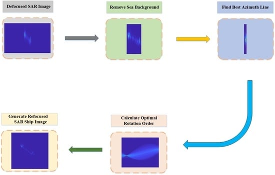
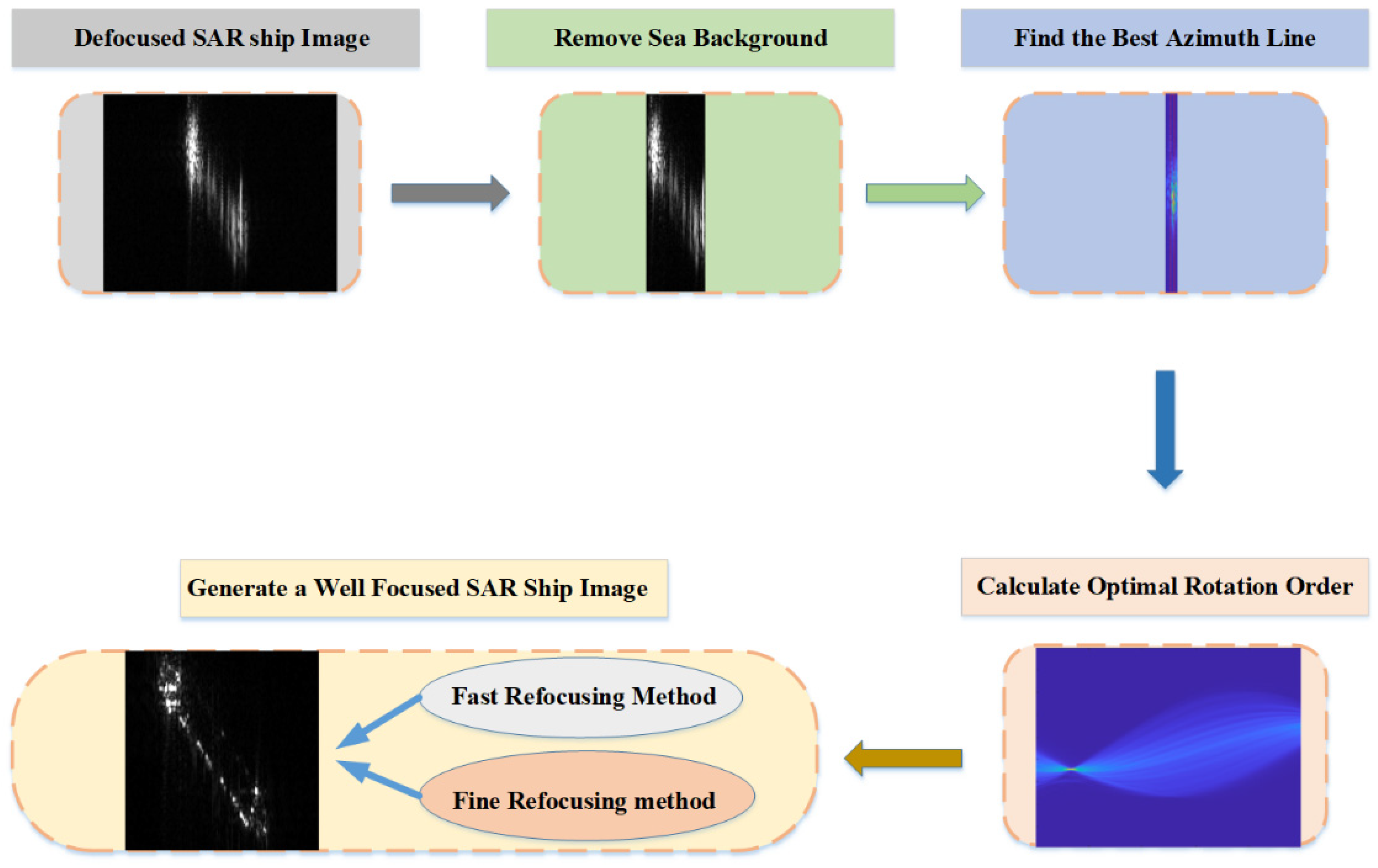
Remotesensing 15 03656 g001
Figure 2. The flowchart of the proposed scheme.
Remotesensing 15 03656 g002
Figure 3. The normalized peak and entropy of one azimuth line after FrFT.
Remotesensing 15 03656 g003
Figure 4. Azimuth profiles of SAR imaging results for different moving states of a point target. (a) Azimuth velocity of 20 m/s. (b) Range acceleration of 10 m/s2. (c) Azimuth acceleration of 15 m/s2.
Remotesensing 15 03656 g004
Figure 5. Time–frequency distribution of signals in different motion states. (a) Azimuth velocity of 20 m/s. (b) Range acceleration of 10 m/s2. (c) Azimuth acceleration of 15 m/s2.
Remotesensing 15 03656 g005
Figure 6. Distribution of signals with different motion states in the FrFT domain. (a) Azimuth velocity of 20 m/s. (b) Range acceleration of 10 m/s2. (c) Azimuth acceleration of 15 m/s2.
Remotesensing 15 03656 g006
Figure 7. The results of the defocused signals with different motion states after FrFT at optimal rotation order. (a) Azimuth velocity of 20 m/s. (b) Range acceleration of 10 m/s2. (c) Azimuth acceleration of 15 m/s2.
Remotesensing 15 03656 g007
Figure 8. The SAR image in Gaofen-3 UFS mode.
Remotesensing 15 03656 g008
Figure 9. Time–frequency distribution of the ship’s best azimuth line. (a) ship1 (b) ship2.
Remotesensing 15 03656 g009
Figure 10. Distribution of the best azimuth line in the FrFT domain. (a) Ship1 (b) Ship2.
Remotesensing 15 03656 g010
Figure 11. Variation of entropy values and peak values with rotation order. (a) Ship1 (b) Ship2.
Remotesensing 15 03656 g011
Figure 12. The result of signal after FrFT at the optimal rotation order. (a) Ship1 (b) Ship2.
Remotesensing 15 03656 g012
Figure 13. Distribution of optimal rotation order for ship’s each azimuth line. (a) Ship1 (b) Ship2.
Remotesensing 15 03656 g013
Figure 14. Distribution in FrFT domain of non-dominant scattering point range cells. (a) Ship1 (b) Ship2.
Remotesensing 15 03656 g014
Figure 15. Image entropy at different range cell’s optimal rotation order. (a) Ship1 (b) Ship2.
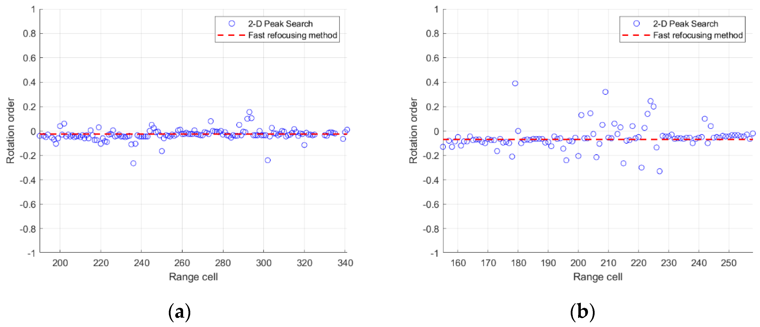
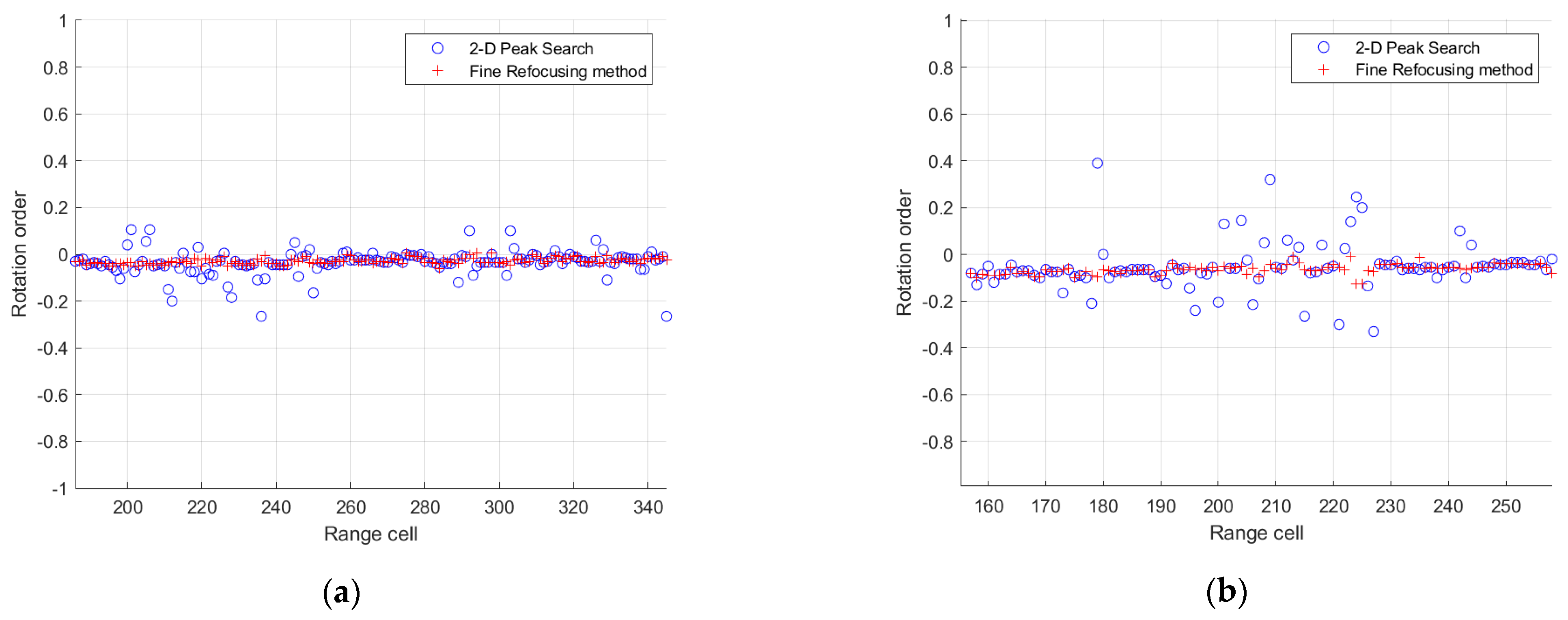
Remotesensing 15 03656 g015
Figure 16. The optimal rotation order of each range cell on the ship obtained by different methods. (a) Ship1. (b) Ship2.
Remotesensing 15 03656 g016
Figure 17. The relationship between the peak and entropy of the signal after FrFT and the rotation order. (a) Ship1. (b) Ship2.
Remotesensing 15 03656 g017
Figure 18. Relationship between the image entropy and the processing time. (a) Ship1. (b) Ship2.
Remotesensing 15 03656 g018
Figure 19. The refocused image of ship1 by different methods. (a) Origin image. (b) PGA. (c) FMEPC. (d) Pelich’s method. (e) Proposed fast refocusing approach. (f) Proposed fine refocusing approach.
Remotesensing 15 03656 g019
Figure 20. The refocused image of ship2 by different methods. (a) Origin image. (b) PGA. (c) FMEPC. (d) Pelich’s method. (e) Proposed fast refocusing approach. (f) Proposed fine refocusing approach.
Remotesensing 15 03656 g020
Figure 21. Six moving ships in Gaofen-3 SL mode.
Remotesensing 15 03656 g021
Figure 22. Time–frequency distribution of each ship’s best azimuth line after STFT. (a) Ship1. (b) Ship2. (c) Ship3. (d) Ship4. (e) Ship5. (f) Ship6.
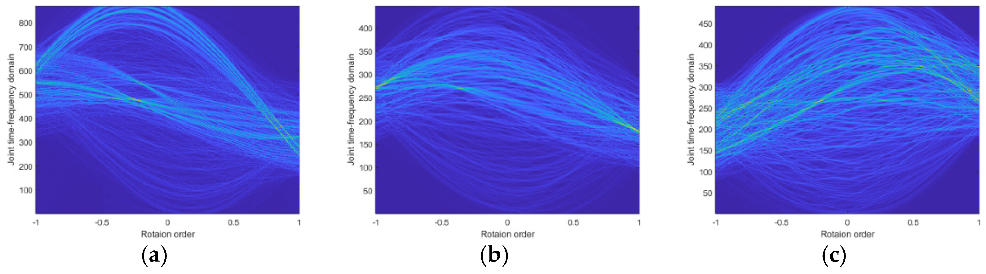
Remotesensing 15 03656 g022
Figure 23. Distribution of each ship’s best azimuth line in the FrFT domain. (a) Ship1. (b) Ship2. (c) Ship3. (d) Ship4. (e) Ship5. (f) Ship6.
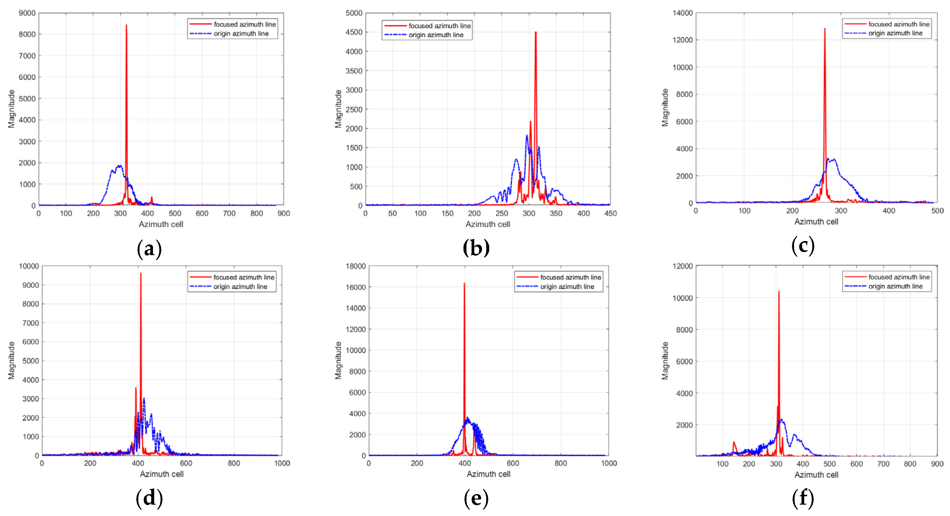
Remotesensing 15 03656 g023
Figure 24. The result of each best azimuth line after FrFT at the optimal rotation order. (a) Ship1. (b) Ship2. (c) Ship3. (d) Ship4. (e) Ship5. (f) Ship6.
Remotesensing 15 03656 g024
Figure 25. Distribution of the optimal rotation order for each range cell. (a) Ship1. (b) Ship2. (c) Ship3. (d) Ship4. (e) Ship5. (f) Ship6.
Remotesensing 15 03656 g025
Figure 26. Distributions of non-dominant scattering point range cells in FrFT domain. (a) Ship1. (b) Ship2. (c) Ship3.
Remotesensing 15 03656 g026
Figure 27. Image entropy at different range cell’s optimal rotation order. (a) Ship1. (b) Ship2. (c) Ship3. (d) Ship4. (e) Ship5. (f) Ship6.
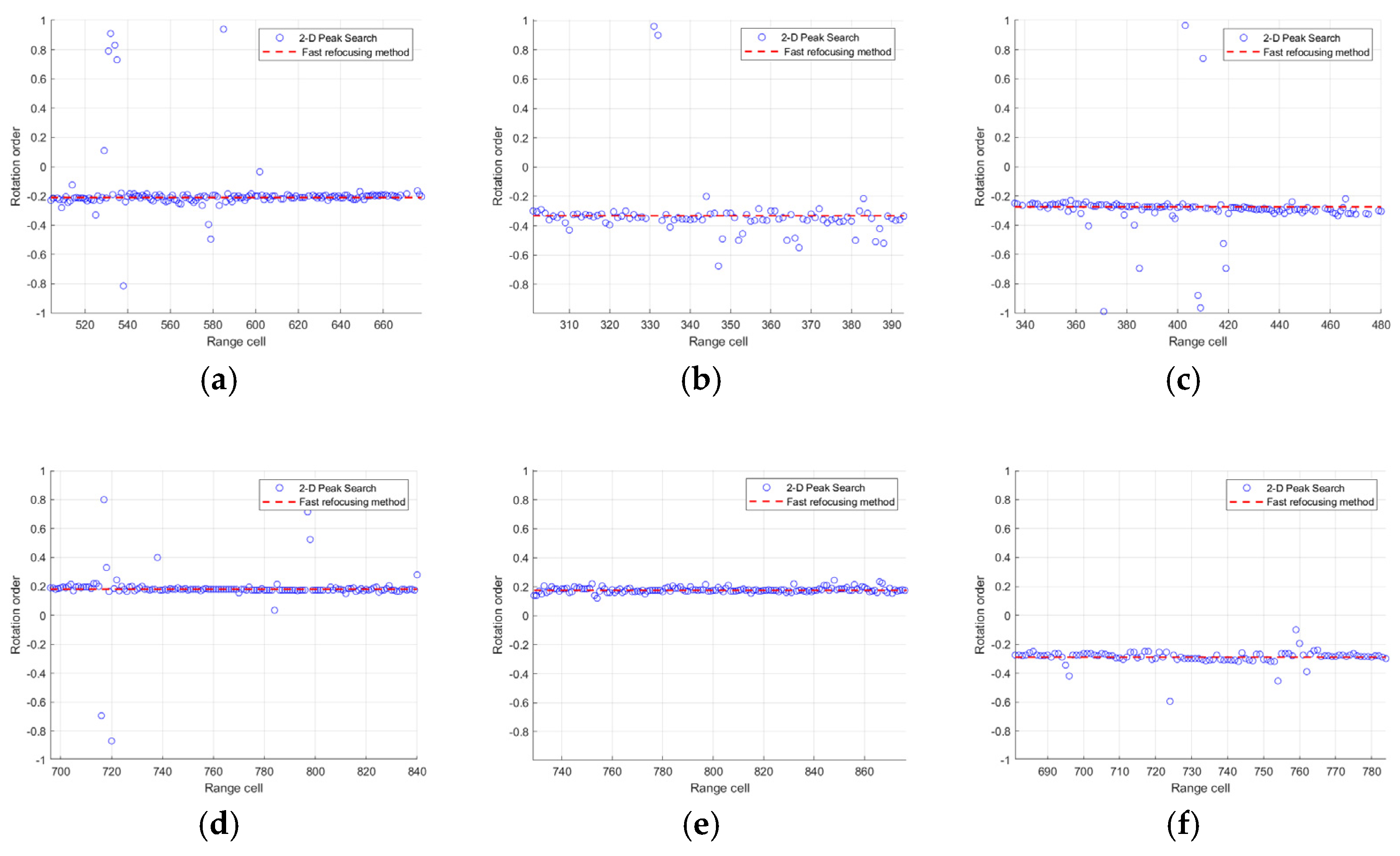
Remotesensing 15 03656 g027
Figure 28. The optimal rotation order of each range cell on the ship obtained by different methods. (a) Ship1. (b) Ship2. (c) Ship3. (d) Ship4. (e) Ship5. (f) Ship6.
Remotesensing 15 03656 g028
Figure 29. Relationship between the entropy and the processing time. (a) Ship1. (b) Ship2. (c) Ship3. (d) Ship4. (e) Ship5. (f) Ship6.
Remotesensing 15 03656 g029
Figure 30. The refocused image of Ship1–Ship6 obtained by different methods which are shown from the first row to the sixth row, respectively. (a) Origin image. (b) Refocused by PGA. (c) Refocused by FMEPC. (d) Refocused by Pelich’s method using FrFT. (e) Refocused by the proposed fast refocusing approach. (f) Refocused by the proposed fine refocusing approach.
Remotesensing 15 03656 g030
Table 1. The SAR system parameters of the simulation experiment.
ParameterValue
Carrier Frequency3 GHZ
Pulse Repetition Frequency188 HZ
Band Width150 MHZ
Platform Height3000 m
Antenna Length2 m
Platform Velocity150 m/s
Pulse Width1.5 μs
Table 2. The numbers of FrFT required for different algorithms.
Proposed Algorithm2D Peak Search Method
Uniform motion in azimuth1260
Acceleration in range1560
Table 3. The SAR system parameters of the Gaofen-3 UFS mode.
ParameterValue
Carrier frequency (GHZ)5.4
Platform velocity (m/s)7568
Band width (MHZ)80
Pulse Width (μs)55
Pulse repetition frequency (Hz)2179
Table 4. The image entropy obtained by different methods.
OriginalPGAFMEPCPelich’s MethodFast RefocusingFine Refocusing
Ship17.917.617.617.67.667.54
Ship25.885.095.085.055.15
Table 5. The processing time of different methods.
PGAFMEPCPelich’s MethodFast RefocusingFine Refocusing
Ship10.53 s3.14 s4.06 s0.085 s0.43 s
Ship20.48 s1.16 s1.2 s0.03 s0.15 s
Table 6. The SAR system parameters of Gaofen-3 SL mode.
ParameterValue
Carrier frequency (GHZ)5.4
Platform velocity (m/s)7567
Band width (MHZ)240
Pulse Width (μs)45
Pulse repetition frequency (Hz)3738
Table 7. The image entropy of different algorithms.
Sub-ImageShip1Ship2Ship3Ship4Ship5Ship6Mean
Original Image9.167.928.359.988.549.558.92
PGA7.516.726.78.587.158.17.46
FMEPC7.56.646.668.577.128.077.43
Pelich’s method using FrFT7.346.566.58.516.587.717.20
Proposed fast refocusing approach7.466.566.628.566.627.967.30
Proposedfine refocusing approach7.356.516.498.526.577.677.18
Table 8. The processing time of different algorithms (in seconds).
Sub-ImageShip1Ship2Ship3Ship4Ship5Ship6Mean
PGA2.050.750.671.623.012.251.73
FMEPC4.461.231.491610.1811.657.50
Pelich’s method using FrFT8.72.63.789.087.054.856.01
Proposed fast refocusing approach0.170.060.110.20.150.10.13
Proposedfine refocusing approach0.90.390.480.850.630.570.64
Disclaimer/Publisher’s Note: The statements, opinions and data contained in all publications are solely those of the individual author(s) and contributor(s) and not of MDPI and/or the editor(s). MDPI and/or the editor(s) disclaim responsibility for any injury to people or property resulting from any ideas, methods, instructions or products referred to in the content.

