
Simulation and Design of an Underwater Lidar System Using Non-Coaxial Optics and Multiple Detection Channels
Abstract
:1. Introduction
2. Principle and Methods
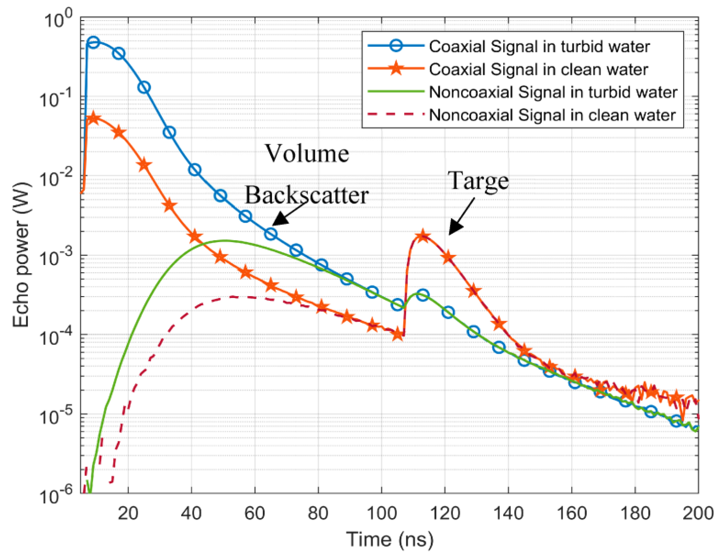
2.1. Principle of the Underwater Lidar
2.2. Simulation Model
2.2.1. Lidar Geometric Model
2.2.2. Multiple Channels Detection Model
3. Description of Underwater Lidar System
4. Simulation and Experimental Results
4.1. Detection Noise Analysis
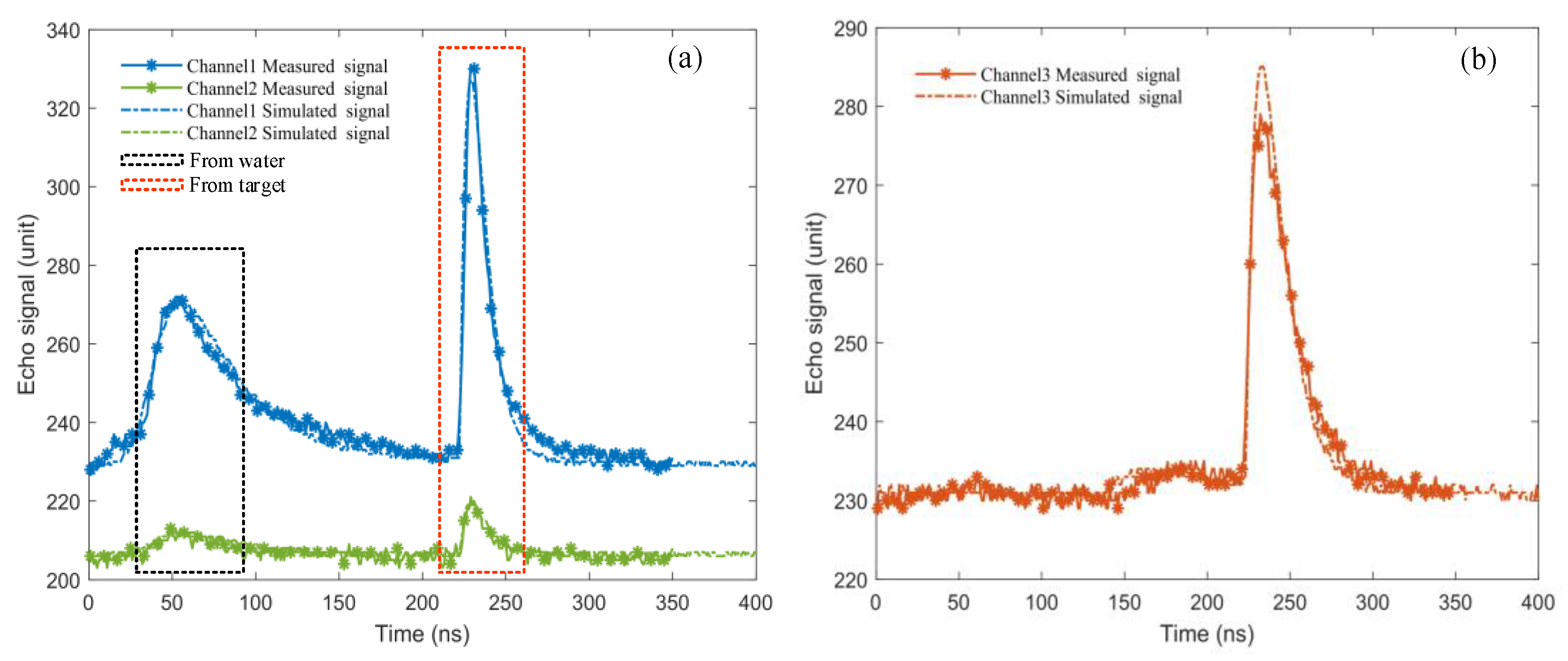
4.2. Anechoic Pond Verification Experiment
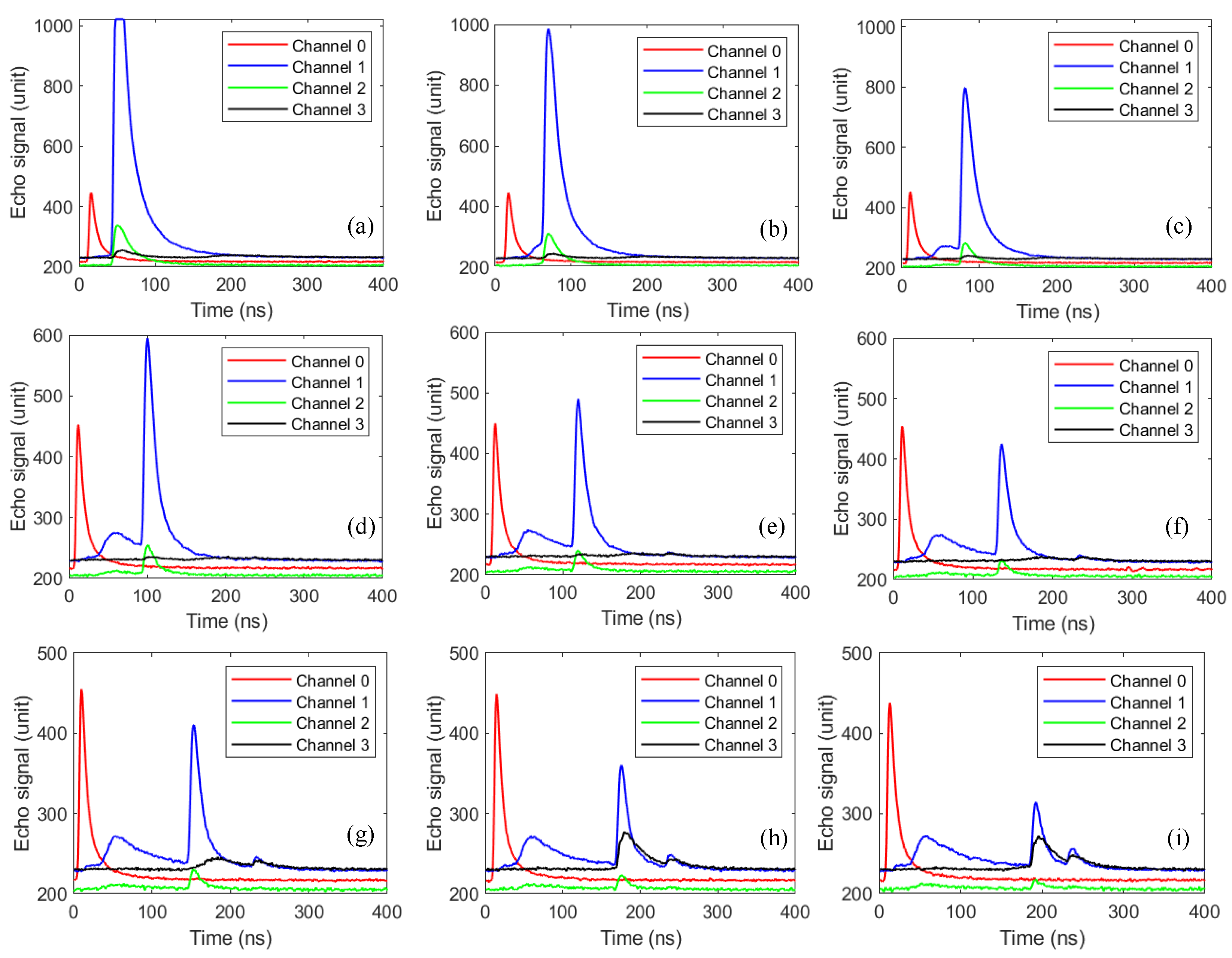
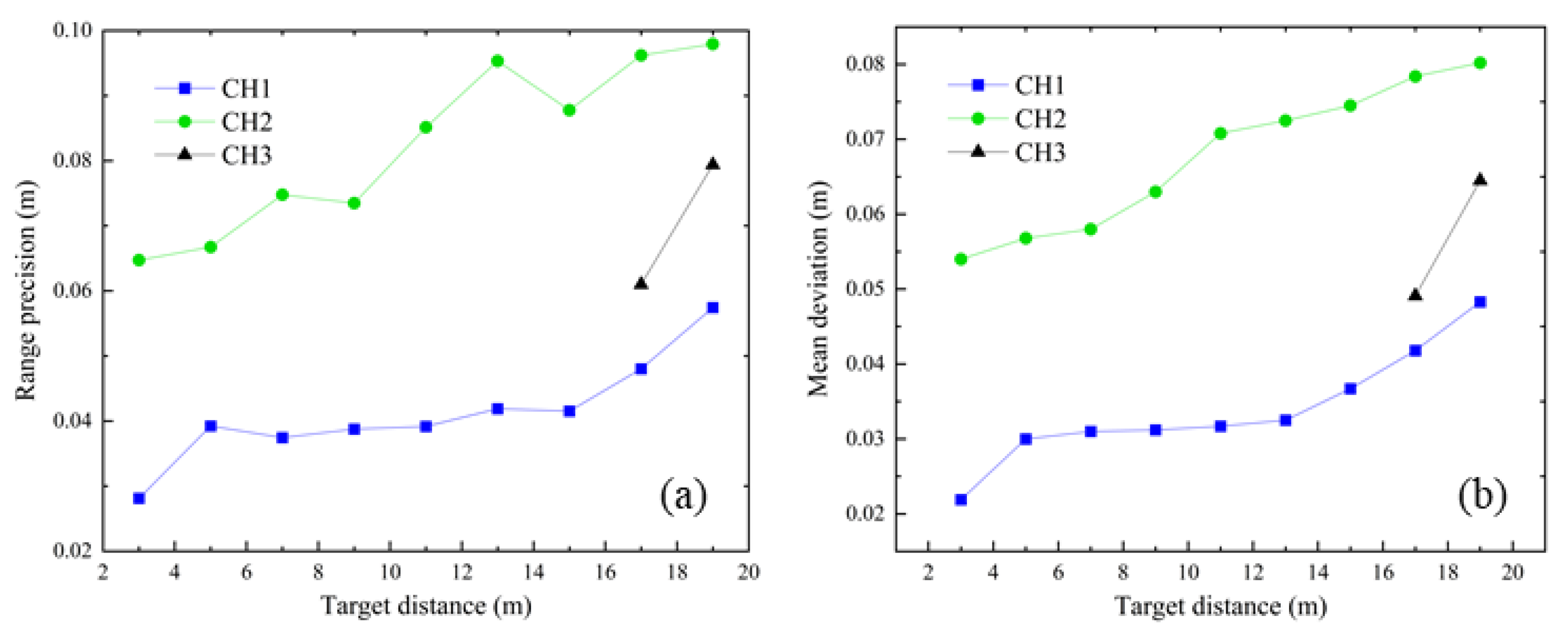
4.3. Swimming Pool Verification Experiment
5. Discussion
6. Conclusions
Author Contributions
Funding
Data Availability Statement
Acknowledgments
Conflicts of Interest
References
- Sun, K.; Cui, W.C.; Chen, C. Review of Underwater Sensing Technologies and Applications. Sensors 2021, 21, 7849. [Google Scholar] [CrossRef]
- Shen, Y.; Zhao, C.A.J.; Liu, Y.; Wang, S.; Huang, F. Underwater Optical Imaging: Key Technologies and Applications Review. IEEE Access 2021, 9, 85500–85514. [Google Scholar] [CrossRef]
- Liu, F.H.; He, Y.; Chen, W.B.; Luo, Y.; Yu, J.Y.; Chen, Y.Q.; Jiao, C.M.; Liu, M.Z. Simulation and Design of Circular Scanning Airborne Geiger Mode Lidar for High-Resolution Topographic Mapping. Sensors 2022, 22, 3656. [Google Scholar] [CrossRef]
- Guo, K.; Li, Q.Q.; Wang, C.S.; Mao, Q.Z.; Liu, Y.X.; Zhu, J.S.; Wu, A.L. Development of a single-wavelength airborne bathymetric LiDAR: System design and data processing. ISPRS J. Photogramm. 2022, 185, 62–84. [Google Scholar] [CrossRef]
- Zhu, Y.D.; Liu, J.Q.; Chen, X.; Zhu, X.P.; Bi, D.C.; Chen, W.B. Sensitivity analysis and correction algorithms for atmospheric CO2 measurements with 1.57-mu m airborne double-pulse IPDA LIDAR. Opt. Express 2019, 27, 32679–32699. [Google Scholar] [CrossRef]
- Wulder, M.A.; Bater, C.W.; Coops, N.C.; Hilker, T.; White, J.C. The role of LiDAR in sustainable forest management. For. Chron. 2008, 84, 807–826. [Google Scholar] [CrossRef] [Green Version]
- Filisetti, A.; Marouchos, A.; Martini, A.; Martin, T.; Collings, S. Developments and applications of underwater LiDAR systems in support of marine science. In Proceedings of the Oceans 2018 Mts/IEEE Charleston, Charleston, SC, USA, 22–25 October 2018. [Google Scholar]
- Zhou, G.; Zhou, X.; Li, W.; Zhao, D.; Song, B.; Xu, C.; Zhang, H.; Liu, Z.; Xu, J.; Lin, G.; et al. Development of a Lightweight Single-Band Bathymetric LiDAR. Remote Sens. 2022, 14, 5880. [Google Scholar] [CrossRef]
- Wang, D.D.; Xing, S.; He, Y.; Yu, J.Y.; Xu, Q.; Li, P.C. Evaluation of a New Lightweight UAV-Borne Topo-Bathymetric LiDAR for Shallow Water Bathymetry and Object Detection. Sensors 2022, 22, 1379. [Google Scholar] [CrossRef]
- Shimada, S.; Takeyama, Y.; Kogaki, T.; Ohsawa, T.; Nakamura, S. Investigation of the Fetch Effect Using Onshore and Offshore Vertical LiDAR Devices. Remote Sens. 2018, 10, 1408. [Google Scholar] [CrossRef] [Green Version]
- Collings, S.; Martin, T.J.; Hernandez, E.; Edwards, S.; Filisetti, A.; Catt, G.; Marouchos, A.; Boyd, M.; Embry, C. Findings from a Combined Subsea LiDAR and Multibeam Survey at Kingston Reef, Western Australia. Remote Sens. 2020, 12, 2443. [Google Scholar] [CrossRef]
- Tulldahl, H.M.; Pettersson, M. Lidar for shallow underwater target detection. Proc. Spie 2007, 6739, 673906. [Google Scholar] [CrossRef]
- McLeod, D.; Jacobson, J.; Hardy, M.; Embry, C. Autonomous Inspection using an Underwater 3D LiDAR. In Proceedings of the 2013 OCEANS, San Diego, CA, USA, 23–27 September 2013. [Google Scholar]
- Liu, Q.; Liu, D.; Zhu, X.L.; Zhou, Y.D.; Le, C.F.; Mao, Z.H.; Bai, J.; Bi, D.C.; Chen, P.; Chen, W.B.; et al. Optimum wavelength of spaceborne oceanic lidar in penetration depth. J. Quant. Spectrosc. 2020, 256, 107310. [Google Scholar] [CrossRef]
- Maccarone, A.; McCarthy, A.; Ren, X.M.; Warburton, R.E.; Wallace, A.M.; Moffat, J.; Petillot, Y.; Buller, G.S. Underwater depth imaging using time-correlated single-photon counting. Opt. Express 2015, 23, 33911–33926. [Google Scholar] [CrossRef]
- Guo, S.C.; He, Y.; Chen, Y.Q.; Chen, W.B.; Chen, Q.; Huang, Y.F. Monte Carlo Simulation with Experimental Research about Underwater Transmission and Imaging of Laser. Appl. Sci. 2022, 12, 8959. [Google Scholar] [CrossRef]
- Churnside, J.H. Review of profiling oceanographic lidar. Opt. Eng. 2013, 53, 051405. [Google Scholar] [CrossRef] [Green Version]
- Churnside, J.H.; Wilson, J.J. Airborne lidar for fisheries applications. Opt. Eng. 2001, 40, 406–414. [Google Scholar] [CrossRef]
- Kokhanenko, G.P.; Penner, I.E.; Shamanaev, V.S. Expanding the dynamic range of a lidar receiver by the method of dynode-signal collection. Appl. Opt. 2002, 41, 5073–5077. [Google Scholar] [CrossRef]
- Imaki, M.; Ochimizu, H.; Tsuji, H.; Kameyama, S.; Saito, T.; Ishibashi, S.; Yoshida, H. Underwater three-dimensional imaging laser sensor with 120-deg wide-scanning angle using the combination of a dome lens and coaxial optics. Opt. Eng. 2017, 56, 031212. [Google Scholar] [CrossRef] [Green Version]
- Sweet, M.H. A Logarithmic Photo-Multiplier Tube Photo-Meter. J. Opt. Soc. Am. 1947, 37, 432–433. [Google Scholar] [CrossRef]
- Churnside, J.H.; Wilson, J.J.; Tatarskii, V.V. Lidar profiles of fish schools. Appl. Opt. 1997, 36, 6011–6020. [Google Scholar] [CrossRef]
- Ooi, J.B.H.; Wong, C.J.; Loh, W.M.E.; Teo, C.K. Numerical Assessment of Horizontal Scanning LIDAR Performance Via Comparative Study Method. Opt. Laser Eng. 2023, 160, 107267. [Google Scholar] [CrossRef]
- Abdallah, H.; Baghdadi, N.; Bailly, J.S.; Pastol, Y.; Fabre, F. Wa-LiD: A New LiDAR Simulator for Waters. IEEE Geosci. Remote Sens. Lett. 2012, 9, 744–748. [Google Scholar] [CrossRef] [Green Version]
- Chen, P.; Jamet, C.; Mao, Z.H.; Pan, D.L. OLE: A Novel Oceanic Lidar Emulator. IEEE Trans. Geosci. Remote 2021, 59, 9730–9744. [Google Scholar] [CrossRef]
- Kim, M.; Kopilevich, Y.; Feygels, V.; Park, J.Y.; Wozencraft, J. Modeling of Airborne Bathymetric Lidar Waveforms. J. Coast. Res. 2016, 76, 18–30. [Google Scholar] [CrossRef]
- Liu, D.; Xu, P.T.; Zhou, Y.D.; Chen, W.B.; Han, B.; Zhu, X.L.; He, Y.; Mao, Z.H.; Le, C.F.; Chen, P.; et al. Lidar Remote Sensing of Seawater Optical Properties: Experiment and Monte Carlo Simulation. IEEE Trans. Geosci. Remote Sens. 2019, 57, 9489–9498. [Google Scholar] [CrossRef]
- Liu, Q.; Cui, X.Y.; Jamet, C.; Zhu, X.L.; Mao, Z.H.; Chen, P.; Bai, J.; Liu, D. A Semianalytic Monte Carlo Simulator for Spaceborne Oceanic Lidar: Framework and Preliminary Results. Remote Sens. 2020, 12, 2820. [Google Scholar] [CrossRef]
- Zhang, Z.H.; Chen, P.; Mao, Z.H. SOLS: An Open-Source Spaceborne Oceanic Lidar Simulator. Remote Sens. 2022, 14, 1849. [Google Scholar] [CrossRef]
- Zhou, G.Q.; Li, C.Y.; Zhang, D.J.; Liu, D.Q.; Zhou, X.; Zhan, J. Overview of Underwater Transmission Characteristics of Oceanic LiDAR. IEEE J. Sel. Top. Appl. Earth Obs. Remote Sens. 2021, 14, 8144–8159. [Google Scholar] [CrossRef]
- Zhou, Y.D.; Chen, W.B.; Cui, X.Y.; Malinka, A.; Liu, Q.; Han, B.; Wang, X.J.; Zhuo, W.Q.; Che, H.C.; Song, Q.J.; et al. Validation of the Analytical Model of Oceanic Lidar Returns: Comparisons with Monte Carlo Simulations and Experimental Results. Remote Sens. 2019, 11, 1870. [Google Scholar] [CrossRef] [Green Version]
- Abdallah, H.; Bailly, J.S.; Baghdadi, N.N.; Saint-Geours, N.; Fabre, F. Potential of Space-Borne LiDAR Sensors for Global Bathymetry in Coastal and Inland Waters. IEEE J. Sel. Top. Appl. Earth Obs. Remote Sens. 2013, 6, 202–216. [Google Scholar] [CrossRef] [Green Version]
- Chen, G.; Tang, J.; Zhao, C.; Wu, S.; Yu, F.; Ma, C.; Xu, Y.; Chen, W.; Zhang, Y.; Liu, J.; et al. Concept Design of the “Guanlan” Science Mission: China’s Novel Contribution to Space Oceanography. Front. Mar. Sci. 2019, 6, 194. [Google Scholar] [CrossRef] [Green Version]
- Shen, X.; Liu, Z.P.; Zhou, Y.D.; Liu, Q.; Xu, P.T.; Mao, Z.H.; Liu, C.; Tang, L.H.; Ying, N.; Hu, M.; et al. Instrument response effects on the retrieval of oceanic lidar. Appl. Opt. 2020, 59, C21–C30. [Google Scholar] [CrossRef]
- Gronwall, C.; Steinvall, O.; Gustafsson, F.; Chevalier, T. Influence of laser radar sensor parameters on range-measurement and shape-fitting uncertainties. Opt. Eng. 2007, 46, 106201. [Google Scholar] [CrossRef] [Green Version]
- Hua, K.J.; Liu, B.; Fang, L.; Wang, H.C.; Chen, Z.; Yu, Y. Detection efficiency for underwater coaxial photon-counting lidar. Appl. Opt. 2020, 59, 2797–2809. [Google Scholar] [CrossRef]
- Zhang, W.H.; Xu, N.; Ma, Y.; Yang, B.S.; Zhang, Z.Y.; Wang, X.H.; Li, S. A maximum bathymetric depth model to simulate satellite photon-counting lidar performance. ISPRS J. Photogramm. 2021, 174, 182–197. [Google Scholar] [CrossRef]
- Henyey, L.G.; Greenstein, J.L. Diffuse radiation in the galaxy. Astrophys. J. 1941, 93, 70–83. [Google Scholar] [CrossRef]
- Guenther, G.; Thomas, R. System Design And Performance Factors For Airborne Laser Hydrography. In Proceedings of the Proceedings OCEANS’83, San Francisco, CA, USA, 29 August–1 September 1983; pp. 425–430. [Google Scholar]
- Chen, Q.; Yam, J.W.; Chua, S.Y.; Guo, N.Q.; Wang, X. Characterizing the performance impacts of target surface on underwater pulse laser ranging system. J. Quant. Spectrosc. 2020, 255, 107267. [Google Scholar] [CrossRef]
- Li, K.P.; He, Y.; Ma, J.; Jiang, Z.Y.; Hou, C.H.; Chen, W.B.; Zhu, X.L.; Chen, P.; Tang, J.W.; Wu, S.H.; et al. A Dual-Wavelength Ocean Lidar for Vertical Profiling of Oceanic Backscatter and Attenuation. Remote Sens. 2020, 12, 2844. [Google Scholar] [CrossRef]
- Zha, B.T.; Yuan, H.L.; Tan, Y.Y. Ranging precision for underwater laser proximity pulsed laser target detection. Opt. Commun. 2019, 431, 81–87. [Google Scholar] [CrossRef]
- Wang, X.Z.; Zhang, M.L.; Zhou, H.Y.; Ren, X.M. Performance Analysis and Design Considerations of the Shallow Underwater Optical Wireless Communication System with Solar Noises Utilizing a Photon Tracing-Based Simulation Platform. Electronics 2021, 10, 632. [Google Scholar] [CrossRef]
- Ehret, G.; Kiemle, C.; Wirth, M.; Amediek, A.; Fix, A.; Houweling, S. Space-borne remote sensing of CO2, CH4, and N2O by integrated path differential absorption lidar: A sensitivity analysis. Appl. Phys. B Laser Opt. 2008, 90, 593–608. [Google Scholar] [CrossRef] [Green Version]
- Eren, F.; Pe’eri, S.; Rzhanov, Y.; Ward, L. Bottom characterization by using airborne lidar bathymetry (ALB) waveform features obtained from bottom return residual analysis. Remote Sens. Environ. 2018, 206, 260–274. [Google Scholar] [CrossRef]
- Solonenko, M.G.; Mobley, C.D. Inherent optical properties of Jerlov water types. Appl. Opt. 2015, 54, 5392–5401. [Google Scholar] [CrossRef]
- Castillon, M.; Palomer, A.; Forest, J.; Ridao, P. State of the Art of Underwater Active Optical 3D Scanners. Sensors 2019, 19, 5161. [Google Scholar] [CrossRef] [Green Version]


| Transmitter | Wavelength λ Pulse energy Et Pulse width Δt Laser repetition rate Beam divergence θt Beam diameter dt | 532 nm 500 μJ 10 ns 5 kHz 2 mrad 10 mm |
| Receiver | Receiver area Ar Geometric offset d Field of view θr Filter bandwidth Δλ Optical efficiency ηo Beam splitter ratio ξi Output signal ratio ξv | 4.4 × 10⁻³ m2 130 mm 50 mrad 1 nm @532 nm 60% 2:98 1:9 |
| Detector | PMT1/PMT2 Detector sensitivity Sk1/Sk2 Max. average anode current Effective area | Non-gated/Gated mode 77/77 mA/W 100/100 μA ∅8/∅8 mm |
| Analog Digital Converter | Bandwidth Sampling rate Resolution Bit Channels | 200 MHz 1 GS/s 10 bits 4 |
| Others | Dimensions Weight Supply voltage | ∅260 mm × 650 mm 30 kg 380 V |
| Target Distance /m | Range Precision/m | Mean Deviation/m | ||||
|---|---|---|---|---|---|---|
| CH1 | CH2 | CH3 | CH1 | CH2 | CH3 | |
| 8.5 | 0.0473 | 0.0664 | 0.0369 | 0.0417 | 0.053 | 0.0279 |
| 10.0 | 0.0674 | 0.0879 | 0.0447 | 0.0557 | 0.0736 | 0.0332 |
| 11.5 | 0.0896 | 0.1085 | 0.0733 | 0.0732 | 0.0931 | 0.0577 |
| Seawater Type | Single-Channel Method (m) | Multiple Channels Strategy | Improvement (Times) | ||
|---|---|---|---|---|---|
| Near-Field (m) | Far-Field (m) | Total (m) | |||
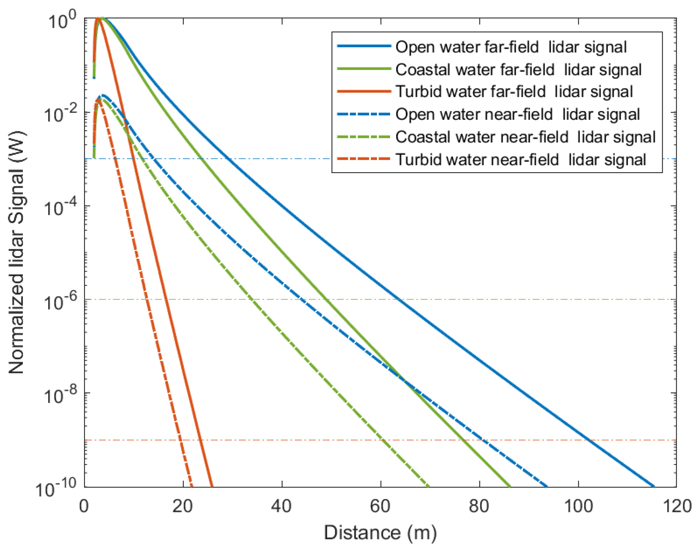
| Clean ocean | 30 | 44 | 44–102 | 102 | 3.4 |
| Coastal ocean | 24 | 34 | 34–76 | 60 | 2.5 |
| Turbid harbor | 10 | 12 | 12–23 | 23 | 2.3 |
Disclaimer/Publisher’s Note: The statements, opinions and data contained in all publications are solely those of the individual author(s) and contributor(s) and not of MDPI and/or the editor(s). MDPI and/or the editor(s) disclaim responsibility for any injury to people or property resulting from any ideas, methods, instructions or products referred to in the content. |
© 2023 by the authors. Licensee MDPI, Basel, Switzerland. This article is an open access article distributed under the terms and conditions of the Creative Commons Attribution (CC BY) license (https://creativecommons.org/licenses/by/4.0/).
Share and Cite
Chen, Y.; Guo, S.; He, Y.; Luo, Y.; Chen, W.; Hu, S.; Huang, Y.; Hou, C.; Su, S. Simulation and Design of an Underwater Lidar System Using Non-Coaxial Optics and Multiple Detection Channels. Remote Sens. 2023, 15, 3618. https://doi.org/10.3390/rs15143618
Chen Y, Guo S, He Y, Luo Y, Chen W, Hu S, Huang Y, Hou C, Su S. Simulation and Design of an Underwater Lidar System Using Non-Coaxial Optics and Multiple Detection Channels. Remote Sensing. 2023; 15(14):3618. https://doi.org/10.3390/rs15143618
Chicago/Turabian StyleChen, Yongqiang, Shouchuan Guo, Yan He, Yuan Luo, Weibiao Chen, Shanjiang Hu, Yifan Huang, Chunhe Hou, and Sheng Su. 2023. "Simulation and Design of an Underwater Lidar System Using Non-Coaxial Optics and Multiple Detection Channels" Remote Sensing 15, no. 14: 3618. https://doi.org/10.3390/rs15143618