Article

A Novel Deep Multi-Image Object Detection Approach for Detecting Alien Barleys in Oat Fields Using RGB UAV Images

1
Finnish Geospatial Research Institute (FGI), National Land-Survey of Finland (NLS), 02150 Espoo, Finland
2
Myyrmäki Campus, School of Smart and Clean Solutions, Metropolia University of Applied Sciences, 01600 Vantaa, Finland
3
Natural Resources Institute Finland (Luke), 00790 Helsinki, Finland
*
Author to whom correspondence should be addressed.
Remote Sens. 2023, 15(14), 3582; https://doi.org/10.3390/rs15143582
Submission received: 30 May 2023 / Revised: 11 July 2023 / Accepted: 15 July 2023 / Published: 17 July 2023
(This article belongs to the Special Issue Novel Applications of UAV Imagery for Forest Science)

Abstract

:
Oat products are significant parts of a healthy diet. Pure oat is gluten-free, which makes it an excellent choice for people with celiac disease. Elimination of alien cereals is important not only in gluten-free oat production but also in seed production. Detecting gluten-rich crops such as wheat, rye, and barley in an oat production field is an important initial processing step in gluten-free food industries; however, this particular step can be extremely time consuming. This article demonstrates the potential of emerging drone techniques for identifying alien barleys in an oat stand. The primary aim of this study was to develop and assess a novel machine-learning approach that automatically detects and localizes barley plants by employing drone images. An Unbiased Teacher v2 semi-supervised object-detection deep convolutional neural network (CNN) was employed to detect barley ears in drone images with a 1.5 mm ground sample distance. The outputs of the object detector were transformed into ground coordinates by employing a photogrammetric technique. The ground coordinates were analyzed with the kernel density estimate (KDE) clustering approach to form a probabilistic map of the ground locations of barley plants. The detector was trained using a dataset from a reference data production site (located in Ilmajoki, Finland) and tested using a 10% independent test data sample from the same site and a completely unseen dataset from a commercial gluten-free oats production field in Seinäjoki, Finland. In the reference data production dataset, 82.9% of the alien barley plants were successfully detected; in the independent farm test dataset, 60.5% of the ground-truth barley plants were correctly recognized. Our results establish the usefulness and importance of the proposed drone-based ultra-high-resolution red–green–blue (RGB) imaging approach for modern grain production industries.

1. Introduction

Oats (Avena sativa), a cereal crop used both by humans as nutrition and as feed for livestock, are primarily cultivated in regions with cold and humid climates in the Northern Hemisphere. They have a wealth of healthy elements, including lipids, proteins, minerals, fiber, and vitamins. Compared to other edible grains, they possess distinctive qualities and a rich nutritional profile [1]. Numerous interventional studies have shown that including oats in a person’s regular diet lowers their chance of developing type 2 diabetes, obesity, hypertension, and all-cause mortality [2]. These studies emphasize the importance of including oats in humans’ everyday diet.
After wheat, maize, rice, barley, and sorghum, oats are the 6th most produced grain worldwide [3]. Global oat production totals 22.7 million metric tons per year [4]. With 7.6 million metric tons produced, the European Union (EU) is the largest oat producer. In the EU countries, Finland ranks among the EU’s top producers with an annual production of 1,100,000 tons, accounting for 11.92% of the bloc’s overall oat production [5].
The absence of gluten, a protein that causes autoimmune reactions in patients with celiac disease, is a significant advantage of pure oats. Food products created from pure oats, such as breakfast cereals, biscuits, and breads, are ideal choices for gluten-intolerant people. The acceptable level of gluten in a gluten-free product is 20 mg/kg [6]. Consuming non-pure oat products, which are contaminated with gluten-rich grains (rye, barley, and wheat), may expose people with celiac disease to the gastrointestinal problems associated with gluten [7]. Worldwide, between 0.5–1.0 percent of all people are gluten intolerant [8]; however, in many nations, including the United States, as many as 6 percent of all people might be gluten intolerant [9]. Contamination of oats with gluten-rich grains can happen during cultivation and harvesting, transportation, and processing [10]. On a typical Finnish contract farm producing gluten-free oats, the cultivation of gluten-rich grains on the same farm is avoided. In crop rotation, the risk of growing gluten-rich crops on the same field parcel is also avoided; however, contamination by alien cereals through the seed material for sowing, seed transportation by birds and animals, and flooding can possibly take place. Gluten-rich species seem very similar to oats during their first stages of growth; however, the differences between them become more obvious at heading when ears emerge in wheat and barley and panicles emerge in oats. Therefore, to implement a uniform oat farming that secures the purity of oat production, a common initial practice is to manually eradicate alien (gluten-rich) species, which typically entails considerable manual labor costs.
Precise detection of alien species plays a critical role in ensuring the consistency of grain products, which is essential for various industries. Gluten-free products are good examples of products that require very strict quality control throughout the entire production process. Usually, a considerable labor cost will be incurred by a farmer to meticulously localize and eradicate alien species two to four times in the course of a growing season. This task involves hours of costly manual labor, which affects the profitability of production. Therefore, manual alien species eradication is a pitfall that affects the competitiveness of gluten-free oat production. This situation could be significantly improved by employing emerging automation technologies in different ways, e.g., new technologies could be employed to accurately localize and eradicate alien species to improve the initial treatment costs for farms. Low-cost capturing platforms such as small unmanned aerial vehicles (UAVs) with red–green–blue (RGB) cameras can play a substantial role in this task, since the small flyers are relatively easy to employ in imaging tasks that can potentially cover a whole farm in a relatively short period of time.
Drones are gradually becoming the de facto data capturing platform for many practical applications. They contain many rapidly developing technologies that are believed to bring new sustainable solutions to outdoor agriculture. Using aerial images to detect trees or plants is a well-known problem in agricultural technology. For example, Wang et al. [11] used an unsupervised classifier to detect single-plant-level cotton from images captured by a drone. They reported that 95.4% of the underlying plants were correctly detected. In their research, sick plants infected by cotton root rot (CRR) were accurately classified at the sub-pixel level. A summarized report of recent studies concerning feature selection methods and resultant waveband selections for hyperspectral sensors for the task of vegetation classification can be found in Hennessy et al. [12]. Rodrigo et al. [13] used the random forest method on hyperspectral data captured by a drone to classify plant communities on a river. Jurišić et al. [14] discussed the potential applications of remote-sensing methods employing drones in crop management. Rosle et al. [6] reviewed UAV-based methods to detect weeds. An open database of 47 plant species that was manually labeled was proposed by Madsen et al. [15]. Zhao et al. [16] used the improved YoloV5 network to detect wheat ears by UAV with an average accuracy of 94.1%.
There exist different approaches for utilizing photogrammetric image blocks in environmental analysis. An image block is formed by collecting overlapping images, and typically composed of several flightlines, with images having overlaps within flightlines as well as between flightlines [17]. Two major approaches for collecting image blocks are nadir views (or integrating nadir) and oblique views [18]. The nadir blocks typically have within- and between-flightlines overlaps of 70–90%, providing 10–30 views covering each object point [19]. The oblique image blocks are often collected in three-dimensional (3D) environments such as cities. The nadir blocks are often processed into orthorectified image mosaics where the most nadir parts of images are used to provide a top view of the object. The oblique datasets are suited for providing realistic 3D views of objects, such as textured 3D models [20]. When investigating plant detection through the utilization of drone data and machine-learning techniques to generate detection maps in real-world coordinates, previous studies have predominantly relied on training classifiers directly using orthomosaic imagery instead of single images (De Castro et al., [21]; Sa et al., [22]). While the effectiveness of this approach has been demonstrated in specific scenarios such as row crops without overlapping plants, it is not well suited for our particular application of detecting barley within an oat field. This discrepancy arises from the distinctive characteristics of the crop and the requirement for a non-nadir view to accurately identify and distinguish the target plants.
Most of the existing classification approaches are unable to feasibly address the complex situation of single plant detection at the ground level, since they mainly concentrate on image level without considering the connectivity of viewing the same object from different angles. In this article, we developed a new semi-supervised approach for detecting barley ears in oat crops to address those gaps. Our method is based on Unbiased Teacher v2 [23] for object detection from a set of multiview images and an image—“Digital Surface Model (DSM)” intersection method for 3D estimation of barley locations. We employed the kernel density estimate (KDE) approach [24] to filter out outliers and create robust 3D estimations from multiple detected coordinates. The main novel points of this article are:
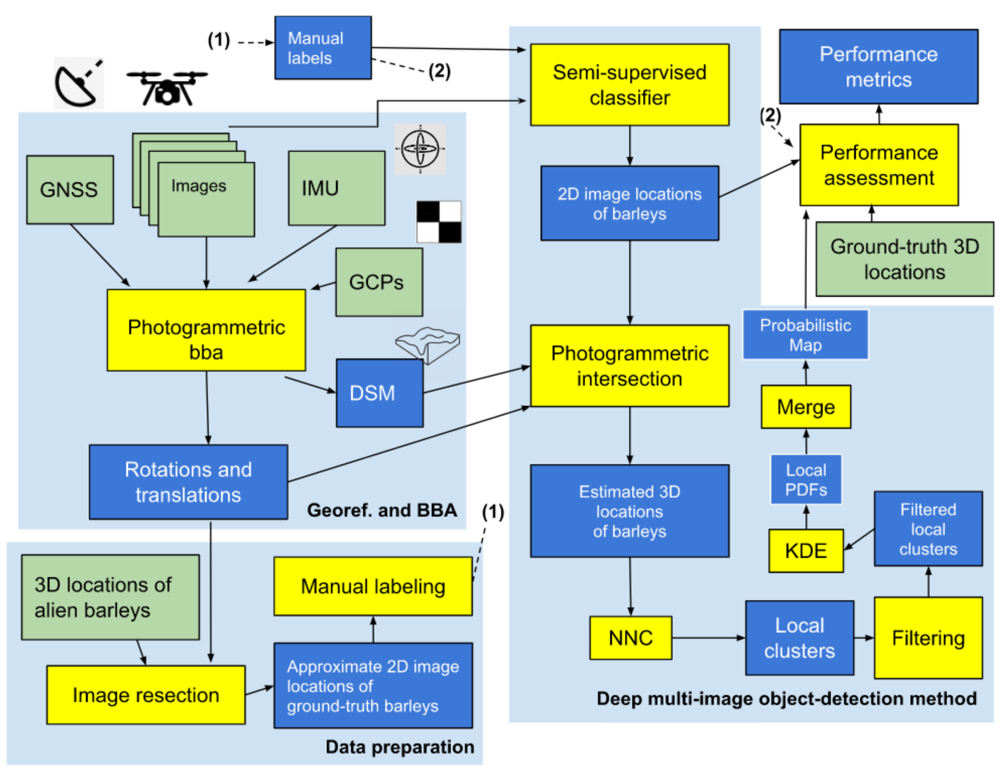
  • Proposing a complete pipeline for detecting the 3D positions of alien barley ears in an oat stand as a probabilistic map;
  • Demonstrating the efficiency of the proposed semi-supervised classifier in detecting barley ears at the image and ground levels;
  • Coupling the image-level estimates with a clustering approach to form a probability density function (PDF) of barley plants as a reliable and robust estimate;
  • Demonstrating the effectiveness of the complete pipeline proposed by applying it to a completely unseen dataset.

2. Deep Multi-Image Object Detection Method

The three primary stages of the proposed multi-view object detection approach are deep multi-image object detection, image annotation, and georeferencing of imagery (Figure 1). The following section is a detailed description of the phases shown in Figure 1.

2.1. Georeferencing

The first step of the proposed method is the georeferencing [25] of images in the photogrammetric block. In this step, a bundle block adjustment (BBA) software is employed to calculate accurate locations and rotations of each image as well as the calibration parameters of the camera. All necessary and optional inputs such as global navigation satellite system (GNSS) and inertial measurement unit (IMU) observations, as well as initial sensor estimations and locations of a few ground control points (GCPs), are fed into the BBA software to estimate an accurate set of positions and orientations for the given sets of images, as well as to gain accurate calibrated sensorial information as the main outputs [17]. The expected output of this part of the pipeline includes a DSM, estimated positions and orientations of images, and calibrated sensor information.

2.2. Annotation

The second phase is image annotation, i.e., detecting and marking the objects of interest with rectangles. The objects are identified in ground inspection and their 3D ground coordinates are measured using an accurate real-time kinematic (RTK) GNSS method. These coordinates are transferred into accurate two-dimensional (2D) image locations of the awns of barley ears by employing collinearity equations. This transformation involves considering a hypothetical cube around each barley ear to eliminate the effect of noise and errors. The outputs of the BBA (accurate positions and orientations of images) are used to project back eight corners of each 3D cube into their corresponding 2D image coordinates by employing the collinearity equation. A rectangular 2D image boundary is then calculated for each barley. The list of rectangular boundaries is visually corrected by a human operator such that only the tail parts of the target barleys remain.

2.3. Deep Multi-Image Object Detection

The third step of the proposed method concerns the foundation of the algorithm. Three important tasks are performed in this section: object detection (Section 2.3.1), ground point estimation (Section 2.3.2), and clustering (Section 2.3.3). In object detection, a semi-supervised object detector is trained to locate barley plants in individual images. The semi-supervised object detector uses annotated training and an unlabeled test dataset to train itself, improve its classification scores, and to self-calibrate (second classification paradigm in Figure 2). The trained classifier is then used to locate barley plants in the test set. In ground point estimation, pixel coordinates of detected barley plants are transformed into 3D ground coordinates by employing a computed photogrammetric DSM. In the clustering phase, the close-by ground points are labeled and converted into individual groups of 3D points. For each cluster, a probabilistic map is produced. Finally, all clusters are combined to form a prediction map.

2.3.1. Semi-Supervised Method: Unbiased Teacher v2

Unbiased Teacher v2 [23] is a framework for semi-supervised object detection. It supports two network architectures: FCOS [26] and Faster R-CNN [27]. We chose to use Faster R-CNN, as it achieved better results in [28]. The advantage of the semi-supervised method over a supervised approach is that additional unlabeled data could potentially be used in the training phase to improve the performance metrics.
The core idea of Unbiased Teacher v2 is training two networks simultaneously, the Student and the Teacher. Initially, in the burn-in stage, a network is trained with the labeled samples only. The weights of the network are copied to the Student and Teacher networks, and the mutual learning stage begins. In every iteration of the mutual learning stage, the Teacher network predicts bounding boxes on unlabeled images, and predictions with a confidence higher than a certain threshold are selected as pseudo-labels that are subsequently employed to train the Student network. The Teacher’s weights are updated as an exponential moving average of the Student’s weights.
Region-based convolutional neural networks (R-CNNs) are a family of object detectors that consist of two stages: region proposal and detection [29]. The region proposal stage extracts potentially interesting regions from an image, and the detection stage classifies each proposed region.
R-CNNs were originally computationally expensive, as each region was treated separately. Fast R-CNN introduced sharing convolutions between proposals, significantly reducing computational cost. Faster R-CNN moves the task of generating proposals to a region proposal network (RPN), a deep convolutional network that shares convolutional layers with the detection network, further improving speed.

2.3.2. Automatic Labeling and 3D-Position Estimation of Unlabeled Barley Plants

The results of the image classification, as a list of image coordinates of barley plants, are fed into a photogrammetric unit for further processing. Here, the aim is to use the outputs of image classification to produce reliable ground estimations of alien barley plants; therefore, image detections are reliably merged into unique ground entities. A valuable tool in the labeling process is the epipolar geometry that helps to accurately eradicate false detections. Moreover, a predefined range for acceptable y-parallaxes is employed to make the object detections ever more robust. Two main approaches can be used: 3D ray intersection and monoplotting [30]; we elected to use the monoplotting option.
3D Localization by DSM Intersection: DSM-based localization is founded upon intersecting spatial rays and the DSM. This model is summarized as,
  • Constituting a linear relationship between an image point and its corresponding focal points of the underlying images;
  • Estimating 3D positions of alien barley plants based on spatial intersection between lines and the DSM. Iterative approach (Figure 3):
    • Considering an approximate plane with a height equal to the average height of the DSM.
    • Finding the intersection between the plane and the line passing by the image point.
    • Projecting back the estimated point on the DSM and estimating a new height.
    • Repeating until the difference between the estimation and the projection becomes small.
  • Intersecting 3D positions on all images to find all possible correspondences for each alien barley plant;
  • Clustering nearby detected positions of each alien barley plant in all images;
  • Filtering out weak clusters based on a criterion such as the number of intersected rays, or acceptable image residuals. The inner part of the mentioned algorithm is depicted in Figure 3.
Compared to the image-based method, this method needs single rays to estimate barley locations. This property leads to a higher number of ground estimates, since multi-ray intersections are usually based on a high number of spatial intersections with low image residuals. The downsides of this approach are a relatively lower reliability and a higher signal-to-noise ratio that needs to be addressed before further analysis.

2.3.3. Clustering Approaches

It is essential to form ground-estimation clusters of the same objects before approximating a PDF for each alien barley plant. Possible locations of alien barleys are estimated by employing the individual ground points calculated by the monoplotting approach (stated in Section 2.3.2). Different approaches could be employed to enable this analysis, e.g., a clustering method such as k-means clustering [31] or self-organizing map (SOM) [32] could be used to join ground points to form separate clusters; alternatively, Gaussian mixture model (GMM) [33], or N-nearest neighbor [34] could be used.
An efficient way to form clusters is by employing the L2 norm in N2 nearest neighbor clustering (NNC). It is therefore a single-parameter approach (one threshold parameter) that could efficiently join close-by 3D estimates. Each initial cluster is formed by considering a local member; gradually, the initial clusters update and merge when unchecked members are considered as potential members based on their closeness to a candidate cluster. The initial clusters are gradually updated to form a list of final clusters.
The final output of the NNC highly depends on the choice of distance measure (Euclidean distance, Manhattan distance, or other similarity metrics), and the threshold parameter that determines the relative closeness of a nominate point to a candidate cluster. The best clustering results are achieved when most of the points are distributed around cluster centroids with sufficient distinctiveness. The clustering result will be noisy and mixed if a considerable amount of salt-and-pepper noise exists, or if traits of mislocated points connect distinctive clusters. Those problems should be addressed, at least to an acceptable extent, by either applying an outlier filtering approach on the noisy data prior to the clustering, or employing a heuristic method to count the number of clusters and estimate cluster centroids.

2.3.4. Kernel Density Estimation (KDE)

The unknown distribution of local clusters is determined by a suitable approach such as KDE [24], where a kernel function such as a Gaussian bell is considered along with a smoothing parameter called bandwidth. The joint PDF of the observed data is finally formed by calculating the cumulative contribution of all the members of a cluster. The resultant PDF is consequently employed to localize the regions where the probability of existence of an alien barley plant is higher. This approach is considered to be non-parametric if the bandwidth is automatically selected, and it could be applied on a finite set of observations. One important property of KDE approach is that it is more suitable to be used to draw inferences about a population, and less suitable for interpolation. Usually, choosing a kernel is not as important as choosing a bandwidth.
A narrow bandwidth could potentially result in a spiky distribution with a higher signal-to-noise ratio (SNR). As the value of bandwidth increases, a higher regularization is applied on the final distribution. Therefore, the bandwidth should be wisely chosen to smooth the output to a desirable extent. The PDF of KDE is stated as
f ^ x = 1 N h i = 1 N K x x i h ,
where N is the number of samples, h is the band width, and summation applies on a local neighborhood.
The input of KDE is a set of distinctive points as a local cluster, and the output is the PDF of the cluster. It is important to emphasize that the list of all 3D points should be clustered before applying KDE. The resultant PDF could be finally normalized according to a criterion such as the number of supporting members. This modification could lower the weights of clusters that have a weakly distributed supporting member.

3. Materials and Method

3.1. Study Area and Reference Data

To facilitate effective reference data capture, a special reference data production trial was established. The oat cultivar ‘Meeri’ was sown at a normal sowing rate of 500 seeds/m2 but we added seeds of the barley cultivar ‘Alvari’ at a rate of 1 and 0.5 seeds/m2 into the seed mixture. The oat stand was established using commercial sowing machinery with 2.5 m working width. A plot border of 30 cm was left unsown between the 70 m long sowing strips to facilitate accurate visual observation and georeferencing of the alien barley plants in the oat stand. The reference data production trial was 0.40 ha which was established on 29 May 2021 in Ilmajoki, Finland. The nitrogen fertilizer application rate was slightly lowered to 80 kg N ha−1 from the suggested rate of around 110 kg N ha−1 to reduce risk of lodging. ‘Meeri’ (Boreal Plant Breeding Ltd., Jokioinen, Finland) and ‘Alvari’ (Boreal Plant Breeding Ltd., Jokioinen, Finland) are cultivars commonly used in Finland of the same earliness level, having 93- and 91-day growing times, respectively. The height of stand at maturity is 94 cm for ‘Meeri’ and 82 cm for ‘Alvari’ [35].
The second field was a commercial gluten-free-oat production field at a farm with an area of 60 m × 165 m (~1 hectare) in Seinäjoki, Finland, that was labeled as the validation field (Figure 4b). This field was sown on the 5 of May 2021 at a sowing rate of 530 seeds/m2 with the ‘Avenue’ (Saadzucht Bauer) cultivar, which is one of the most common cultivars for gluten-free oat production in Finland. The fertilizer application rate was 130 kg nitrogen ha−1. ‘Avenue’ is a late cultivar with an estimated growing time of 101 days and a height of 94 cm.
In the test parcels, a careful survey was carried out to detect all barley plants in the oat stands. The survey was done during the same day as the image capture was carried out. As the barley cultivars head earlier than oat cultivars, the optimum time for image capture and for weeding is a two-week time period after barley heading (when the awns become visible) and before the oat panicles emerge. As the oat cultivars grow taller than the barley cultivars, many of the barley plants disappear into the oat stand later in the season and cannot be easily recognized by either human eyes inside a field or drone images.
In the reference data production trial, a total number of 524 barleys were detected during the field survey and their locations were measured using the Topcon Hiper HR RTK GNSS receiver. A total number of 50 alien barley plants were detected and localized in the validation field. In general, the horizontal positional accuracy of barley plants was ~2 cm in both fields. The approximated height of barley plants was considered as 30 cm. More specifically, the position where the stem comes out of the ground (site at which the plant is rooted) was located, which does not give an accurate position of the ear as the stem is typically tilted and the ear part bent. In practice, these uncertainties were tackled in the annotation phase by interactively annotating the precise positions of the ears. In total, 21 GCPs were observed in the reference field and 4 GCPs were observed in the validation field. The reference data production trial was harvested on 7 September 2021. Five 1-row meter samples of the oat stand produced an estimate that the oat stand had on average 387 oat plants and 433 oat panicles m2. Yield estimation calculated by harvesting a sample plot of 15 m2 was 4024 kg ha−1 (at 86% dry matter), which was higher than the average oat yield for the region (3100 kg ha−1) stated in the national yield statistics [36].

3.2. Drone Data

A Matrice M300RTK drone (manufactured by DJI) was employed to capture aerial photos of the farms. The drone was equipped with a Zenmuse P1 RGB camera (8192 px by 5460 px), a dual-frequency GNSS receiver, and an IMU sensor (Figure 5). The average flying height of the drone was 12 m above ground level. The flight was carried out in the “Smart oblique Capture” mode, which acquires oblique images to the left, right, back, and front directions using 66 degrees of tilt angle, in addition to nadir images. The data collection of the reference dataset in Ilmajoki took place on 9 July 2021 at 14:00 local time (UTC +2:00). The whole experimental field was captured in 56 min. The ground sampling distance was 1.5 mm at the center of the image at nadir direction. The sky was sunny, and the solar zenith angle was 42 degrees. Similar settings were used to collect data on the validation farm on 29 June 2021 at 10:00 local time (UTC +2:00) with a clear sky and a solar zenith angle of 53 degrees.
In total, 2495 images were captured by the RGB camera in the training field. From the whole dataset, 2304 images were processed in the BBA. A dense point cloud was generated using the estimated camera positions and the dense image matching technique. A DSM with a ground sample distance (GSD) of 1 cm was computed from the dense point cloud. From the processed dataset, a total of 1495 images were selected based on visibility of the ground-truth barley observations. The images were divided into eight subsets, seven (0th–6th) of which contained 200 sub-images, and one (7th) which contained 95 sub-images. This dataset of eight subsets was called the reference dataset. Three parts of the reference dataset (parts 0th, 6th, and 7th) were manually labeled. Figure 6 shows examples of two alien barley plants. The awns of the barley plants are localized in this figure. Overall, 495 of the 1495 images were manually labeled using Labelme software [27]. The rest of the dataset (1st–5th) was used for testing (1000 images).

3.3. Labeling and Classification

All the rectangular image sections of the reference dataset were manually corrected in 495 images using the Labelme software [27], such that the tail part was meticulously targeted. The original large images (8192 × 5460 pixels) were divided into 72 smaller patches (~910 × 682 pixels).
The data pool of the reference dataset consisted of
-
3463 labeled patches;
-
72,000 unlabeled patches;
-
274 labeled patches reserved as a test set.
The reference dataset was split into a training set and a test set. Approximately 90% of the reference dataset was considered as the training set, and the remaining 10% was considered as an independent test set (Figure 7). The training and test samples were uniformly selected by a randomized process on image level. The validation dataset was kept completely separated from the training process to demonstrate the usefulness of the trained classifier on a greater scale. Consequently, the method was assessed by employing two separate test datasets.

3.4. Implementation Details

In the geo-referencing and BBA section, Agisoft Metashape software (version 2.0.2) [37] was employed to process the image data. The output of Metashape was processed by a Python 3.9 script to create appropriate input for Labelme as json text files. The boundaries were converted into rectangular shapes and saved as json text files. The results of Labelme were processed by a Python 3.9 script for the semi-supervised classifier.
The semi-supervised method, Unbiased Teacher v2, was trained on ITC Center for Science Ltd. (CSC, Bengaluru, India) Mahti cluster [38]. All modifications made to Unbiased Teacher v2′s code, along with the scripts for running it on Mahti, are available at [23]. Mahti uses the Slurm workload manager [39], meaning that a resource reservation and running time estimate must be provided when launching a job. Unbiased Teacher v2 was trained on a single node with four Nvidia A100 GPUs. Training took 18 h with a batch size of 32. A total number of 20,000 iterations were executed, of which the first 5000 iterations constituted the fully supervised burn-in stage. All details are available in the GitHub repository of our fork of Unbiased Teacher v2 [23].
The estimated 3D coordinates of the alien barley plants were clustered by the NNC method described in (Section 2.3.3) using a MATLAB R2022b script. Each local cluster was fed into the KDE module to approximate local PDFs. The KDE approach was implemented in MATLAB as local and global estimators. Several more MATLAB R2022b scripts were implemented for DSM intersections and clustering. All PDFs were merged to form a global probabilistic map that was used to estimate the performance metrics of Section 3.5. For georeferencing, a few GCPs were employed to estimate an Affine transformation. The GDAL 3.6.2 library [40] was employed inside Python 3.9 to save the georeferencing parameters of the estimated Affine transformation. QGIS 3.24.2 was employed for map visualization and plotting. The results were assessed and plotted inside MATLAB R2022b and Python 3.9.

3.5. Performance Metrics

To demonstrate the effectiveness of our proposed method, two sets of performance metrics were considered. The first set concerned the object-level detections, including true positive rate ( T P R ) and overall accuracy. Those metrics were employed to demonstrate the efficiency of the PDF estimator to localize alien barley plants on the farms [41]. T P R is calculated as
T P R = T P T P + F N
where T P is the number of true positives, and F N is the number of false negatives. T P R is also called recall. Overall accuracy is calculated as
A c c u r a c y = T P + T N n P + n N
where T N is the number of true negatives, n P is the number of positives, and n N is the number of negatives. P r e c i s i o n is calculated as
P r e c i s i o n = T P T P + F P
where F P is the number of false positives.
The second set consisted of average precision ( A P ) [42] and average recall ( A R ), which assessed the performance of the object detectors at the image level. Average precision is calculated as
A P X = i = 1 N P r e c i s i o n i X N
where N is the number of images, and P r e c i s i o n i X is the precision of the i t h image at the intersection over union ( I o U ) of X . Average recall ( A R ) is calculated as
A R X = i = 1 N R e c a l l i X N
where R e c a l l i X is the recall of the i t h image at the I o U of X . Both A P and A R were reported at an I o U of 50% as A P 50 and A R 50 .

4. Results

4.1. Image-Level Detection

The semi-supervised object detector was successfully trained by a stochastic gradient-based approach. Two examples of successfully detected barleys are shown from different views in Figure 8 and Figure 9. It is visible in these figures that the barley ears look different from each viewpoint. Therefore, a sufficient amount of training cases seemed to be necessary to train a qualified object detector.
The patches containing barley ears were relatively difficult to localize manually inside the images. The ears of barley were visible only when there was a considerable difference between the background and a barley ear, as depicted in Figure 8. In this figure, the same barley is shown from eight different views. It is obvious from Figure 8 that the ear of the plant is distinguishable with both geometric and radiometric differences from its neighboring matured oats. The color of the barley has a yellow component that makes it different from the “forest green” of matured oats. The shape of the ear is spiky and it can be differentiated from the oats if it is viewed from the correct angle from an appropriate distance. The size of barley ears was significantly different in images, since oblique imaging geometry was used, and consequently the GSD was not uniform over the whole image. The human operator was able to localize most of the desired barley ears; however, detecting a significant portion of them was assumed to be very difficult due to the problems that were caused by parameters such as similarity in texture information between barleys and oats, occlusion, or large distance to the cameras. A false positive case is shown in Figure 10. The image residual of this case was low; therefore, it was classified as a barley, but it is a false detection based on the appearance of the weed. A case with high confidence (>90%) is shown in Figure 9. It is possible to visually recognize the ear of the plant in this figure. As the confidence number increases, the visual appearance of the detected plants slightly improves.
The performance metrics of the trained object detectors for the training and test sets are presented in Table 1. All the following metrics were reported at IoU = 50%. For the semi-supervised method, the AP50 of the classifier was 97.7% on the Ilmajoki training set and 95.2% on the Ilmajoki test set. The output of the image classifier contained the location of detected barleys along with a confidence number. Overall, the performance of the trained classifier was considered acceptable for the project; however, there was a considerable amount of false image detections. Verifying the correctness of automatically detected barley plants was difficult for a human operator since, even if some of the detected patches were located on correct positions, no simple visual mark existed to confirm the detection. Most of the false image detections were removed when a high confidence threshold of 90% was used to filter out image detections with lower confidence. For each image detection, the center of the detected rectangle was projected back to the ground.
Inference speed for the original (8192 × 5460) images was 3.9 s per image after cutting them into smaller tiles, which took 1.2 s/img, totalling 5.1 s/img.

4.2. Object-Level Detection at Trial Site

Figure 11 shows the 3D object points (alien barleys) in a local neighborhood obtained by the image–DSM intersection algorithm (Section 2.3.2). The manually obtained positions of alien barley plants are plotted as pink points. All manually obtained points with a corresponding cluster of image-based approximation are surrounded by yellow rectangles. Clusters of estimations that did not correspond to a manually measured 3D point are surrounded by red rectangles. Figure 11 reveals that the set of 3D manual measurements does not contain all actual alien barley plants in the field, showing that many alien barley plants failed to be found by the human operator. This is due to the difficult measurement conditions on the farm. The figure highlights the importance of using the proposed method to complete the manual measurement.
Figure 12 shows the effect of employing different confidence thresholds on reducing the number of outliers from image detection tasks. Local clusters are formed in the figure by employing NNC with norm L2, and they can be seen plotted as red circles. From left to right, the acceptance threshold level is gradually increased from 20% to 60%. The rightmost figure has an acceptance threshold level of 80%. It is obvious from this figure that the confidence number of the image classifier is correlated to the possibility of points being outliers.
Results of the NNC method using the L2 norm (Section 2.3.3) are plotted in Figure 13. The input 3D points were filtered out before the clustering step by considering a relatively high threshold of 90% for the confidence score of the image detections. Therefore, local clusters are relatively clear for the clustering method. Each cluster is painted with a random color in the figure. It is obvious from Figure 13 that the barley plants were well separated. Clusters with a small number of members could be immediately assigned as outliers and filtered out. Clusters with a sufficient number of members (>5) were fed into the KDE algorithm. The result of KDE as a PDF of the alien barley plants is plotted in Figure 14. On the left side of Figure 14, the PDF is overlaid with supporting point estimates (as red points) and manually measured barleys (as yellow points). The right side demonstrates a magnification of a small local neighborhood of the PDF. Figure 15 shows the final PDF as the probabilistic estimate that is overlaid on the DSM. The search region for detecting alien barleys could be seen to be significantly limited. Approximately <3% of the pixel values are marked as alien barley plants. It is possible that a region contains more than one barley plant as a result. Overall, 82.9% of the ground-truth alien barley plants were correctly detected. Figure 16 demonstrates a magnification of a small region in the field. The shape of the local neighborhoods is according to the selection of the kernel, as can be seen in this figure. The output of KDE was binarized by considering different thresholds (20–80%). For each threshold, a TPR value was calculated. The TPR values with respect to the acceptance threshold for the reference dataset are plotted in Figure 17. According to this figure, 90.48% TPR was achieved for the threshold 20%.

4.3. Object-Level Detection at the Test Site

The classifier trained using the Ilmajoki training dataset was employed to determine locations of barley plants in the test dataset. Figure 18 shows a successfully detected barley plant from 10 different views in this dataset. On the right side of this figure, the corresponding local cluster and the PDF are plotted. The left side of Figure 19 shows a local neighborhood with five correctly detected barleys. On the right side of this figure, two undetected barleys are shown. Overall, 60.5% of all manually measured barleys were localized by the trained classifier.

5. Discussion

Automatic recognition of alien barley plants in an oat stand was demonstrated as a complex vision task that requires employing state-of-the-art image classification methods as well as photogrammetric techniques. The underlying classification problem was addressed by combining the results of a semi-supervised classification method with a clustering approach. The success of the proposed algorithm was demonstrated by detecting the majority of the target objects at ground level in two real oat production fields. The concept of employing a semi-supervised classifier was demonstrated as an appropriate sub-solution for the specific situation of the underlying problem. The results of the semi-supervised classifier were aligned with previous studies such as [43,44]. A desirable property of the Unbiased Teacher V2 semi-supervised object detector in localizing target patterns within image boundaries enabled us to localize alien barley plants precisely inside images; therefore, precise ground-level localization became achievable. The photogrammetric ray–DSM intersection led to accurate ground-level results; however, a considerable amount of noise was observed. Ground estimates of the manually measured barley plants were also scattered to a noticeable extent; therefore, employing the KDE clustering method was essential to unify the estimates and remove the weakly detected barleys and outliers.
The performance of our proposed method was astonishingly acceptable on the reference dataset. The state-of-the-art object detection algorithm was able to correctly recognize alien barley plants in an image even when it seemed very difficult or impossible for a human operator. This was due to the complex structure of the classification problem. In many cases, the target patch was very similar to the background.
An acceptable performance of the complete barley-detection module was successfully demonstrated in a separate validation dataset that had a slightly different capturing situation. In this case, the oat cultivar ‘Avenue’ was used, while in the reference dataset ‘Meeri’ was used. Similarly, the image capture took place 55 days after sowing for the validation data, while in the reference dataset the difference was 41 days from sowing. Although ‘Avenue’ is a later cultivar than ‘Meeri’, the development of the oat stand was more advanced in the validation dataset. In addition, the added alien barley plants were of one cultivar in the training and the first validation set, but the alien plants in the Seinäjoki validation set were of an unknown cultivar, although they were barley plants. A drop in classification accuracy was observed for the validation dataset. The difference between the classification accuracy of the test part of the reference dataset and that of the validation dataset was expected, since the condition of the two fields was slightly different. One reason for why the detection might have been more difficult in the real farm dataset was that some alien barleys were lower in comparison to the oats, so they might not have been clearly visible, especially from oblique images. This was likely due to the more advanced development of the oat stand. Despite the difference, the proposed method was proven to be helpful even in that case.
The novel method already showed very good operational performance in the test farm. To further improve the performance, more datasets collected in different conditions are needed, including, e.g., different illumination conditions, different relative sizes of the main and alien crops, and different spectral crop characteristics. Considering the computational efficiency in terms of computing times and required GPU/CPU, improvements are still needed. The dataset was huge, as the image ground resolution was 1.6 mm and multiple images per object points were used. Training and inference were computationally intensive. The subsequent monoplotting and clustering procedures, on the other hand, were computationally efficient. However, in practical applications, inference would preferably be carried out during flying; thus, efficient algorithms should be implemented to carry out detection using onboard computers; examples of efficient implementations are the recent YOLO architectures [45].

6. Conclusions

The proposed method solved the limitations of the current image classification methods by combining photogrammetric and clustering methods. The final product as a probabilistic map of the densities of barleys is valuable in terms of prediction power. In conclusion, coupling the image-based barley detector with the KDE method through the photogrammetric intersection of space rays and DSM was proven to be a successful tool in recognizing barleys and filtering the outliers. Our work highlights the potential and usefulness of state-of-the-art deep-learning-based object detectors in the automation task of localizing plants on a modern farm. In addition to gluten-free oat production, the method can also be applied to the seed production of cereals in which the number of seeds of other cereal species is restricted, as well as in malting barley production.

Author Contributions

Conceptualization, E.K. and E.H.; methodology, E.K., S.R., A.P. and E.H.; software, E.K., S.R. and A.P.; validation, E.K., S.R., R.N., R.A.O. and E.H.; investigation, E.K., R.N. and S.R.; resources, E.H., R.N., O.N. and M.N; writing—original draft preparation, E.K.; writing—review and editing, E.K., R.N., S.R., R.A.O., O.N., M.N. and E.H.; visualization, E.K. and R.A.O.; supervision, E.H.; project administration, E.H.; funding acquisition, O.N. and E.H. All authors have read and agreed to the published version of the manuscript.

Funding

This research was financially supported by the Identification of unwanted cultivated species in seed multiplication and in gluten free oat cultivation “DrooniLuuppina” project number 144989 funded by the European Agricultural Fund for Rural Development (EAFRD), and the Academy of Finland ICT 2023 Smart-HSI—“Smart hyperspectral imaging solutions for new era in Earth and planetary observations” (Decision no. 335612). This research was carried out in affiliation with the Academy of Finland Flagship “Forest-Human-Machine Interplay—Building Resilience, Redefining Value Networks and Enabling Meaningful Experiences (UNITE)” (Decision no. 337127) ecosystem.

Acknowledgments

We would like to thank all of the farmers who allowed us to carry out measurements in their fields. Arja Nykänen from SeAMK is thanked for her co-operation at the Ilmajoki trial site. Additionally, we would like to thank Juho Kotala from ProAgria, and Niko Koivumäki, Helmi Takala, and Teemu Hakala from the National Land Survey of Finland, for their support during the project.

Conflicts of Interest

The authors declare no conflict of interest. The funders had no role in the design of the study; in the collection, analyses, or interpretation of data; in the writing of the manuscript; or in the decision to publish the results.

References

  1. Butt, M.S.; Tahir-Nadeem, M.; Khan, M.K.I.; Shabir, R.; Butt, M.S. Oat: Unique among the Cereals. Eur. J. Nutr. 2008, 47, 68–79. [Google Scholar] [CrossRef]
  2. Varma, P.; Bhankharia, H.; Bhatia, S. Oats: A Multi-Functional Grain. J. Clin. Prev. Cardiol. 2016, 5, 9. [Google Scholar] [CrossRef]
  3. Stevens, E.J.; Armstrong, K.W.; Bezar, H.J.; Griffin, W.B.; Hampton, J.G. Fodder Oats an Overview. Fodd. Oats World Overv. 2004, 33, 11–18. [Google Scholar]
  4. Production of Oats Worldwide 2022/2023. Available online: https://www.statista.com/statistics/1073536/production-of-oats-worldwide/ (accessed on 11 May 2023).
  5. Leading Oats Producers Worldwide 2022 | Statista. Available online: https://www.statista.com/statistics/1073550/global-leading-oats-producers/ (accessed on 11 May 2023).
  6. Rosle, R.; Che’Ya, N.N.; Ang, Y.; Rahmat, F.; Wayayok, A.; Berahim, Z.; Fazlil Ilahi, W.F.; Ismail, M.R.; Omar, M.H. Weed Detection in Rice Fields Using Remote Sensing Technique: A Review. Appl. Sci. 2021, 11, 10701. [Google Scholar] [CrossRef]
  7. Green, P.H.; Cellier, C. Celiac Disease. N. Engl. J. Med. 2007, 357, 1731–1743. [Google Scholar] [CrossRef] [PubMed]
  8. Fasano, A.; Araya, M.; Bhatnagar, S.; Cameron, D.; Catassi, C.; Dirks, M.; Mearin, M.L.; Ortigosa, L.; Phillips, A. Federation of International Societies of Pediatric Gastroenterology, Hepatology, and Nutrition Consensus Report on Celiac Disease. J. Pediatr. Gastroenterol. Nutr. 2008, 47, 214–219. [Google Scholar] [CrossRef] [PubMed] [Green Version]
  9. Akter, S. Formulation of Gluten-Free Cake for Gluten Intolerant Individuals and Evaluation of Nutritional Quality. PhD Thesis, Chattogram Veterinary and Animal Sciences University, Chattogram, Bangladesh, 2020. [Google Scholar]
  10. Erkinbaev, C.; Henderson, K.; Paliwal, J. Discrimination of Gluten-Free Oats from Contaminants Using near Infrared Hyperspectral Imaging Technique. Food Control 2017, 80, 197–203. [Google Scholar] [CrossRef]
  11. Wang, T.; Thomasson, J.A.; Isakeit, T.; Yang, C.; Nichols, R.L. A Plant-by-Plant Method to Identify and Treat Cotton Root Rot Based on UAV Remote Sensing. Remote Sens. 2020, 12, 2453. [Google Scholar] [CrossRef]
  12. Hennessy, A.; Clarke, K.; Lewis, M. Hyperspectral Classification of Plants: A Review of Waveband Selection Generalisability. Remote Sens. 2020, 12, 113. [Google Scholar] [CrossRef] [Green Version]
  13. da Silva, A.R.; Demarchi, L.; Sikorska, D.; Sikorski, P.; Archiciński, P.; Jóźwiak, J.; Chormański, J. Multi-Source Remote Sensing Recognition of Plant Communities at the Reach Scale of the Vistula River, Poland. Ecol. Indic. 2022, 142, 109160. [Google Scholar] [CrossRef]
  14. Jurišić, M.; Radočaj, D.; Šiljeg, A.; Antonić, O.; Živić, T. Current Status and Perspective of Remote Sensing Application in Crop Management. J. Cent. Eur. Agric. 2021, 22, 156–166. [Google Scholar] [CrossRef]
  15. Leminen Madsen, S.; Mathiassen, S.K.; Dyrmann, M.; Laursen, M.S.; Paz, L.-C.; Jørgensen, R.N. Open Plant Phenotype Database of Common Weeds in Denmark. Remote Sens. 2020, 12, 1246. [Google Scholar] [CrossRef] [Green Version]
  16. Zhao, J.; Zhang, X.; Yan, J.; Qiu, X.; Yao, X.; Tian, Y.; Zhu, Y.; Cao, W. A Wheat Spike Detection Method in UAV Images Based on Improved YOLOv5. Remote Sens. 2021, 13, 3095. [Google Scholar] [CrossRef]
  17. Gerke, M.; Przybilla, H.-J. Accuracy Analysis of Photogrammetric UAV Image Blocks: Influence of Onboard RTK-GNSS and Cross Flight Patterns. Photogramm. Fernerkund. Geoinf. PFG 2016, 1, 17–30. [Google Scholar] [CrossRef] [Green Version]
  18. Rossi, P.; Mancini, F.; Dubbini, M.; Mazzone, F.; Capra, A. Combining Nadir and Oblique UAV Imagery to Reconstruct Quarry Topography: Methodology and Feasibility Analysis. Eur. J. Remote Sens. 2017, 50, 211–221. [Google Scholar] [CrossRef] [Green Version]
  19. Nesbit, P.R.; Hugenholtz, C.H. Enhancing UAV–SFM 3D Model Accuracy in High-Relief Landscapes by Incorporating Oblique Images. Remote Sens. 2019, 11, 239. [Google Scholar] [CrossRef] [Green Version]
  20. Aicardi, I.; Chiabrando, F.; Grasso, N.; Lingua, A.M.; Noardo, F.; Spanò, A. Uav Photogrammetry with Oblique Images: First Analysis on Data Acquisition and Processing. Int. Arch. Photogramm. Remote Sens. Spat. Inf. Sci. 2016, 41, 835–842. [Google Scholar] [CrossRef] [Green Version]
  21. De Castro, A.I.; Torres-Sánchez, J.; Peña, J.M.; Jiménez-Brenes, F.M.; Csillik, O.; López-Granados, F. An Automatic Random Forest-OBIA Algorithm for Early Weed Mapping between and within Crop Rows Using UAV Imagery. Remote Sens. 2018, 10, 285. [Google Scholar] [CrossRef] [Green Version]
  22. Sa, I.; Popović, M.; Khanna, R.; Chen, Z.; Lottes, P.; Liebisch, F.; Nieto, J.; Stachniss, C.; Walter, A.; Siegwart, R. WeedMap: A Large-Scale Semantic Weed Mapping Framework Using Aerial Multispectral Imaging and Deep Neural Network for Precision Farming. Remote Sens. 2018, 10, 1423. [Google Scholar] [CrossRef] [Green Version]
  23. Liu, Y.-C.; Ma, C.-Y.; Kira, Z. Unbiased Teacher v2: Semi-Supervised Object Detection for Anchor-Free and Anchor-Based Detectors. In Proceedings of the IEEE/CVF Conference on Computer Vision and Pattern Recognition, New Orleans, LA, USA, 18–24 June 2022; pp. 9819–9828. [Google Scholar]
  24. Silverman, B.W. Using Kernel Density Estimates to Investigate Multimodality. J. R. Stat. Soc. Ser. B Methodol. 1981, 43, 97–99. [Google Scholar] [CrossRef]
  25. Štroner, M.; Urban, R.; Reindl, T.; Seidl, J.; Brouček, J. Evaluation of the Georeferencing Accuracy of a Photogrammetric Model Using a Quadrocopter with Onboard GNSS RTK. Sensors 2020, 20, 2318. [Google Scholar] [CrossRef] [PubMed] [Green Version]
  26. Tian, Z.; Shen, C.; Chen, H.; He, T. Fcos: Fully Convolutional One-Stage Object Detection. In Proceedings of the IEEE/CVF International Conference On Computer Vision, Seoul, Republic of Korea, 27 October–2 November 2019; pp. 9627–9636. [Google Scholar]
  27. Ren, S.; He, K.; Girshick, R.; Sun, J. Faster R-Cnn: Towards Real-Time Object Detection with Region Proposal Networks. Adv. Neural Inf. Process. Syst. 2015, 28. [Google Scholar] [CrossRef] [Green Version]
  28. Bochkovskiy, A.; Wang, C.-Y.; Liao, H.-Y.M. Yolov4: Optimal Speed and Accuracy of Object Detection. arXiv 2020, arXiv:2004.10934. [Google Scholar]
  29. Girshick, R.; Donahue, J.; Darrell, T.; Malik, J. Region-Based Convolutional Networks for Accurate Object Detection and Segmentation. IEEE Trans. Pattern Anal. Mach. Intell. 2015, 38, 142–158. [Google Scholar] [CrossRef] [PubMed]
  30. Karras, G.E.; Patias, P.; Petsa, E. Digital Monoplotting and Photo-Unwrapping of Developable Surfaces in Architectural Photogrammetry. Int. Arch. Photogramm. Remote Sens. 1996, 31, 290–294. [Google Scholar]
  31. Likas, A.; Vlassis, N.; Verbeek, J.J. The Global K-Means Clustering Algorithm. Pattern Recognit. 2003, 36, 451–461. [Google Scholar] [CrossRef] [Green Version]
  32. Kohonen, T. The Self-Organizing Map. Proc. IEEE 1990, 78, 1464–1480. [Google Scholar] [CrossRef]
  33. Reynolds, D.A. Gaussian Mixture Models. Encycl. Biom. 2009, 741, 659–663. [Google Scholar]
  34. Fu, A.W.; Chan, P.M.; Cheung, Y.-L.; Moon, Y.S. Dynamic Vp-Tree Indexing for n-Nearest Neighbor Search given Pair-Wise Distances. VLDB J. 2000, 9, 154–173. [Google Scholar] [CrossRef]
  35. Results of Official Variety Trials 2015–2022. Available online: https://px.luke.fi:443/PxWebPxWeb/pxweb/en/maatalous/maatalous__lajikekokeet__julkaisuvuosi_2022__sato__kaura/150100sato_kaura.px/ (accessed on 30 May 2023).
  36. Viljelykasvien Sato Muuttujina Vuosi, ELY-Keskus, Tieto, Tuotantotapa Ja Kasvilaji. Available online: https://statdb.luke.fi/PxWeb/pxweb/fi/LUKE/LUKE__02%20Maatalous__04%20Tuotanto__14%20Satotilasto/01_Viljelykasvien_sato.px/ (accessed on 30 May 2023).
  37. Cutugno, M.; Robustelli, U.; Pugliano, G. Structure-from-Motion 3d Reconstruction of the Historical Overpass Ponte Della Cerra: A Comparison between Micmac® Open Source Software and Metashape®. Drones 2022, 6, 242. [Google Scholar] [CrossRef]
  38. Markomanolis, G.S.; Alpay, A.; Young, J.; Klemm, M.; Malaya, N.; Esposito, A.; Heikonen, J.; Bastrakov, S.; Debus, A.; Kluge, T. Evaluating GPU Programming Models for the LUMI Supercomputer. In Proceedings of the Supercomputing Frontiers: 7th Asian Conference, SCFA 2022, Singapore, 1–3 March 2022; Springer International Publishing: Cham, Switzerland, 2022; pp. 79–101. [Google Scholar]
  39. Iserte, S.; Prades, J.; Reaño, C.; Silla, F. Increasing the Performance of Data Centers by Combining Remote GPU Virtualization with Slurm. In Proceedings of the 2016 16th IEEE/ACM International Symposium on Cluster, Cloud and Grid Computing (CCGrid), Cartagena, Colombia, 16–19 May 2016; pp. 98–101. [Google Scholar]
  40. Warmerdam, F. The Geospatial Data Abstraction Library. In Open Source Approaches in Spatial Data Handling; Spinger: Berlin/Heidelberg, Germany, 2008; pp. 87–104. [Google Scholar]
  41. Grandini, M.; Bagli, E.; Visani, G. Metrics for Multi-Class Classification: An Overview. arXiv 2020, arXiv:200805756. [Google Scholar]
  42. Henderson, P.; Ferrari, V. End-to-End Training of Object Class Detectors for Mean Average Precision. In Proceedings of the Computer Vision–ACCV 2016: 13th Asian Conference on Computer Vision, Taipei, Taiwan, 20–24 November 2016, Revised Selected Papers, Part V 13; Springer: Berlin/Heidelberg, Germany, 2017; pp. 198–213. [Google Scholar]
  43. Zhang, C.; Cheng, J.; Tian, Q. Unsupervised and Semi-Supervised Image Classification with Weak Semantic Consistency. IEEE Trans. Multimed. 2019, 21, 2482–2491. [Google Scholar] [CrossRef]
  44. Liu, B.; Yu, X.; Zhang, P.; Tan, X.; Yu, A.; Xue, Z. A Semi-Supervised Convolutional Neural Network for Hyperspectral Image Classification. Remote Sens. Lett. 2017, 8, 839–848. [Google Scholar] [CrossRef]
  45. GitHub—Ultralytics/Ultralytics: NEW—YOLOv8 🚀 in PyTorch > ONNX > CoreML > TFLite. Available online: https://github.com/ultralytics/ultralytics (accessed on 30 May 2023).
Figure 1. Overview of the proposed method. Measurements, modules, and outputs are plotted in green, yellow, and blue boxes, respectively. The photogrammetric core is grouped on the left side. Dashed lines with numbers show long-distance connections. (GNSS = Global Navigation Satellite System, IMU = Inertial Measurement Unit, GCPs = Ground Control Points, DSM = Digital Surface Model, BBA = Bundle Block Adjustment, NNC = Nearest Neighbor Clustering, KDE = Kernel Density Estimation, PDF= Probability Density Function).
Remotesensing 15 03582 g001
Figure 2. Two training and classification paradigms. On the top is the classic classification paradigm; on the bottom is the concurrent training, classification, and calibration paradigm.
Remotesensing 15 03582 g002
Figure 3. Iteratively estimating the intersection of an image ray and digital surface model (DSM) by employing accurate orientation and position of images.
Remotesensing 15 03582 g003
Figure 4. (a) The reference (Ilmajoki) dataset. (b) The validation (Seinäjoki) dataset. The green points represent the locations of the manually measured alien barley plants. Brown rectangles in (a) are image projection of the training images.
Remotesensing 15 03582 g004
Figure 5. DJI Matrice M300RTK UAV.
Remotesensing 15 03582 g005
Figure 6. Examples of two alien barley plants in a sample image. The awns of the barley ears make them recognizable. X and Y axes are pixel coordinates.
Remotesensing 15 03582 g006
Figure 7. The training and the test sets of the reference (Ilmajoki) dataset. The boundaries of training images are plotted in red color. The green part in the middle is the test set. The test ground-truth barleys are plotted in yellow.
Remotesensing 15 03582 g007
Figure 8. A successful case of an automatically labeled barley (no. 5) from 8 supporting views. Blue texts plotted at the center are pixel coordinates of corresponding blue crosses.
Remotesensing 15 03582 g008
Figure 9. A high-confidence case (confidence > 0.9) of an automatically labeled barley (no. 177) from 9 supporting views. Blue texts plotted at the center are pixel coordinates of corresponding blue crosses.
Remotesensing 15 03582 g009
Figure 10. Cases of outliers of automatic image-based detection. Blue texts plotted at the center are pixel coordinates of corresponding blue crosses.
Remotesensing 15 03582 g010
Figure 11. Intersecting image locations of estimated alien barleys with DSM (confidence > 90%). Yellow rectangles are ground-truth barleys. Red rectangles are possible locations of newly detected barleys.
Remotesensing 15 03582 g011
Figure 12. Effect of confidence number on reducing the number of outliers. From left to right, points with 20%, 60%, and 80% confidence are plotted. Local clusters are plotted as red points. Green points are single detections. White points are ground truth.
Remotesensing 15 03582 g012
Figure 13. Individual clusters of supporting points.
Remotesensing 15 03582 g013
Figure 14. Geographic probability density function (PDF) of alien barleys overlaid with 3D object points (red points) and manual measurements (yellow points) in black and white [0–1] probability. The right side is a magnification of a small portion of the PDF. Threshold was 20%.
Remotesensing 15 03582 g014
Figure 15. Probability distribution of detected alien barleys (prediction map) based on kernel density estimate (KDE).
Remotesensing 15 03582 g015
Figure 16. Probability distribution of detected alien barleys (prediction map) for a small local neighborhood.
Remotesensing 15 03582 g016
Figure 17. True positive ratio (TPR) curve with respect to varying confidence threshold values for the reference dataset.
Remotesensing 15 03582 g017
Figure 18. A positive case on the validation dataset (Seinäjoki). Blue texts plotted at the center are pixel coordinates of corresponding blue crosses.
Remotesensing 15 03582 g018
Figure 19. Results of clustering on the validation dataset. The kernel density estimate (KDE) clusters are plotted in red, estimated ground positions of barleys are in yellow, and manually measured barleys are in green.
Remotesensing 15 03582 g019
Table 1. Average precision of the object detector on the Ilmajoki dataset, at IoU = 50%.
DatasetUnlabeled DataAP50AR50
TrainNo95.2%99.6%
TrainYes97.7%100.0%
TestNo94.5%98.0%
TestYes95.8%98.3%
Disclaimer/Publisher’s Note: The statements, opinions and data contained in all publications are solely those of the individual author(s) and contributor(s) and not of MDPI and/or the editor(s). MDPI and/or the editor(s) disclaim responsibility for any injury to people or property resulting from any ideas, methods, instructions or products referred to in the content.

