Article

UAV-Based Terrain Modeling in Low-Vegetation Areas: A Framework Based on Multiscale Elevation Variation Coefficients

1
School of Remote Sensing & Geomatics Engineering, Nanjing University of Information Science & Technology, Nanjing 211800, China
2
School of Geographical Sciences, Nanjing University of Information Science & Technology, Nanjing 211800, China
3
Institute of Earth Surface Dynamics (IDYST), University of Lausanne, 1015 Lausanne, Switzerland
4
Changwang School of Honors, Nanjing University of Information Science & Technology, Nanjing 211800, China
*
Author to whom correspondence should be addressed.
Remote Sens. 2023, 15(14), 3569; https://doi.org/10.3390/rs15143569
Submission received: 29 May 2023 / Revised: 10 July 2023 / Accepted: 14 July 2023 / Published: 16 July 2023

Abstract

:
The removal of low vegetation is still challenging in UAV photogrammetry. According to the different topographic features expressed by point-cloud data at different scales, a vegetation-filtering method based on multiscale elevation-variation coefficients is proposed for terrain modeling. First, virtual grids are constructed at different scales, and the average elevation values of the corresponding point clouds are obtained. Second, the amount of elevation change at any two scales in each virtual grid is calculated to obtain the difference in surface characteristics (degree of elevation change) at the corresponding two scales. Third, the elevation variation coefficient of the virtual grid that corresponds to the largest elevation variation degree is calculated, and threshold segmentation is performed based on the relation that the elevation variation coefficients of vegetated regions are much larger than those of terrain regions. Finally, the optimal calculation neighborhood radius of the elevation variation coefficients is analyzed, and the optimal segmentation threshold is discussed. The experimental results show that the multiscale coefficients of elevation variation method can accurately remove vegetation points and reserve ground points in low- and densely vegetated areas. The type I error, type II error, and total error in the study areas range from 1.93 to 9.20%, 5.83 to 5.84%, and 2.28 to 7.68%, respectively. The total error of the proposed method is 2.43–2.54% lower than that of the CSF, TIN, and PMF algorithms in the study areas. This study provides a foundation for the rapid establishment of high-precision DEMs based on UAV photogrammetry.

1. Introduction

Unmanned aerial vehicles (UAVs) play an important role in digital terrain modeling [1,2,3,4]. They support fast and accurate terrain modeling in small areas, thus reducing the typical cost and workload. However, UVA photogrammetry can only provide digital surface models (DSMs). A digital elevation model (DEM) constructed with terrain modeling requires the removal of surface features, such as vegetation [5]. The quality and accuracy of a DEM are determined by the accuracy of surface-feature removal or by the precision of ground-point selection. In nature, most surface features are vegetation. Thus, the accuracy of terrain modeling is influenced by the accuracy of vegetation removal. Especially in areas with complex topography, the continuity and inconsistency of topographic undulations and the inconsistency of the density and height of vegetation, particularly the presence of low vegetation, increase the complexity of terrain modeling. Rapid and accurate removal of vegetation areas is a key issue in DEM construction [6].
Many point-cloud filtering algorithms have been used for identifying ground points and nonground points (such as vegetation). These point-cloud filtering algorithms can be mainly classified as the morphological method [7,8], triangulated irregular network-based (TIN-based) algorithms [9], machine-learning-based algorithms [10], and mathematical morphology-based algorithms [11,12].
The morphological method filters off-ground points according to the morphological characteristics of terrain surface, such as terrain slope [7], curvature [7], and simulation of a virtual surface [8]. For example, cloth simulation filtering (CSF) filters off-ground points by simulating a cloth overlaid on terrains [13]. CSF works effectively in flat areas, but the results are not satisfactory in areas with complex terrain, such as both flat and steep slopes [14]. The morphological method is generally simple and efficient but does not perform well in areas with complex terrain, especially in areas with rugged terrain and low vegetation cover [15]. The TIN-based method gradually approximates the ground surface by iteratively selecting ground points from seed points and densifies a sparse TIN. Whether a ground point is selected is determined by its angle and distance from the seed point. This method yields a better filtering effect in urban areas than other methods do and can adapt to areas with topographic discontinuity, but the method is ineffective in mountainous areas with more vegetation cover [16]. The machine-learning-based approach simplifies the filtering process to a point-cloud binary classification problem. First, a point-cloud classification model is established, and the model is used to complete the labeling of sample ground points and nonground points. Although these methods can achieve good accuracy, the pretraining samples are labor-intensive to label and train, and the generalization performance is inadequate [13,17]. Mathematical morphology-based algorithms apply open and closed operations to images [12]. The filtering process is completed based on changes in image characteristics. The most important aspect of this method is the choice of the filtering window scale. Large objects cannot be effectively removed when the window scale is small, and terrain detail is easily missed when it is large.
Different point-cloud filtering algorithms have distinct advantages and disadvantages for different terrain features and areas [18]. However, these methods are mainly based on the morphological characteristics of terrain surfaces at a unique scale [19,20]. The characteristics of the ground and nonground points at different spatial scales are distinctly different [21,22,23]. Only considering the morphological characteristics of terrain surfaces at a unique scale makes it difficult to achieve high accuracy. In recent years, researchers have proposed various improved filtering methods to address this inadequacy [24]. A parameter-free progressive TIN densification algorithm was developed to make the selection of thresholds in progressive TIN densification more flexible and adaptive to fit complex terrain features [8]. Additionally, an improved simple morphological filter was established using a linearly increasing window and simple slope thresholding to address morphological filter inadequacies at a single scale [25,26]. However, these improved multiscale filtering methods generally extract morphological characteristics at different scales and then combine them to identify ground points [27]. The differences in surface features at different scales are not directly considered.
If point-cloud data are integrated at different scales through a virtual grid (VG), the elevation values produced will be associated with a range of variations. This degree of variation reflects the surface characteristics (e.g., vegetation and topography) that are reflected in the point cloud at different scales. If the degree of elevation variation in point-cloud data at different scales can be quantified, a new approach to terrain modeling could be developed. The elevation variation coefficient (EVC) is an important topographic factor in digital terrain analysis [28,29]. Notably, it can be used to quantify the degree of elevation variation within neighborhood units. Therefore, this paper aims to develop a terrain modeling framework based on multiscale elevation-variation coefficients in low-vegetation areas.

2. Materials and Methods
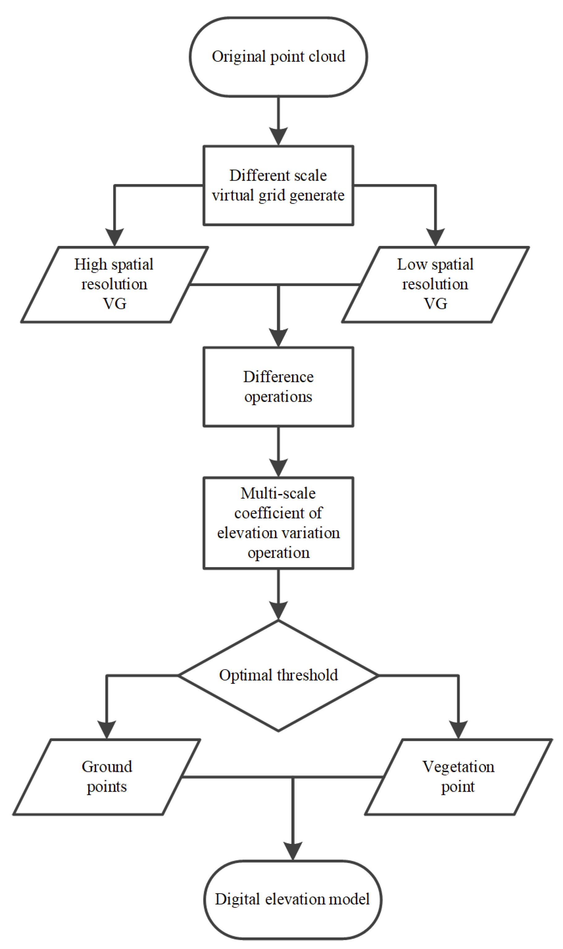
2.1. Overview

The terrain features in point-cloud data at different scales vary significantly. For example, point-cloud data with a high spatial resolution (average sampling interval) can not only accurately express the terrain, but can also encompass other features, such as low vegetation, while low-spatial-resolution point-cloud data can only represent large-scale topographic relief. If the original high-precision point-cloud data are used to generate virtual grids (VGs) at different scales, a series of changes (variations) will occur in the elevation values of the VGs, especially in vegetated areas, with elevation variations that may be inaccurate. However, ground points and vegetation points can potentially be differentiated by quantifying the degree of elevation variation at different scales. The methodological flowchart of the approach proposed in this study is shown in Figure 1. First, a multiscale VG was established. The average elevation value of all points in the VG was calculated to assign an elevation attribute value to the VG. Second, the elevation changes of VGs were obtained based on difference operations. Then, the window shape and focal information were used to calculate the standard deviation and mean, the ratio of which was the elevation variation coefficient (EVC) of each grid. Finally, a threshold was selected to discriminate between ground points and vegetation points.

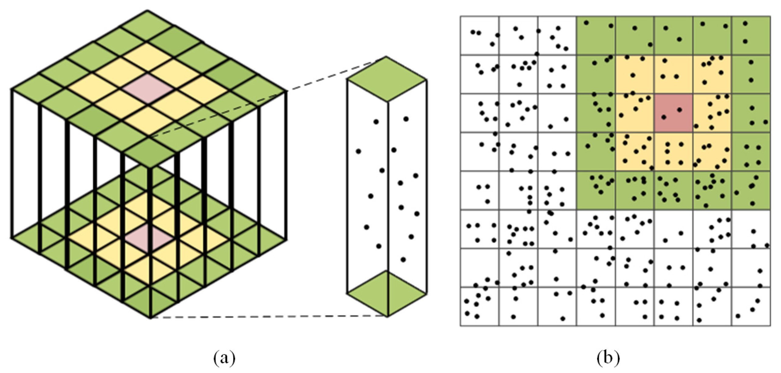
2.2. Multiscale Virtual Grid Generation

To improve the accuracy of ground-point selection, multiscale VGs are introduced in this paper. Regular VGs are composed of multiple cubes of equal length and width (Figure 2). First, three-dimensional regular VGs were generated, and the point clouds were included in the corresponding cube according to their coordinates (Figure 2a). Then, the point clouds were segmented with a grid approach, and each grid contained several elevation points. The different scales of the VGs were represented by different colors (Figure 2b). The elevation of each VG was determined according to the average of the points’ elevation. The large-scale VGs played a role in smoothing the terrain and obtaining elevation values. The elevation values obtained by the small-scale VGs were similar to the actual elevation of the ground surface.

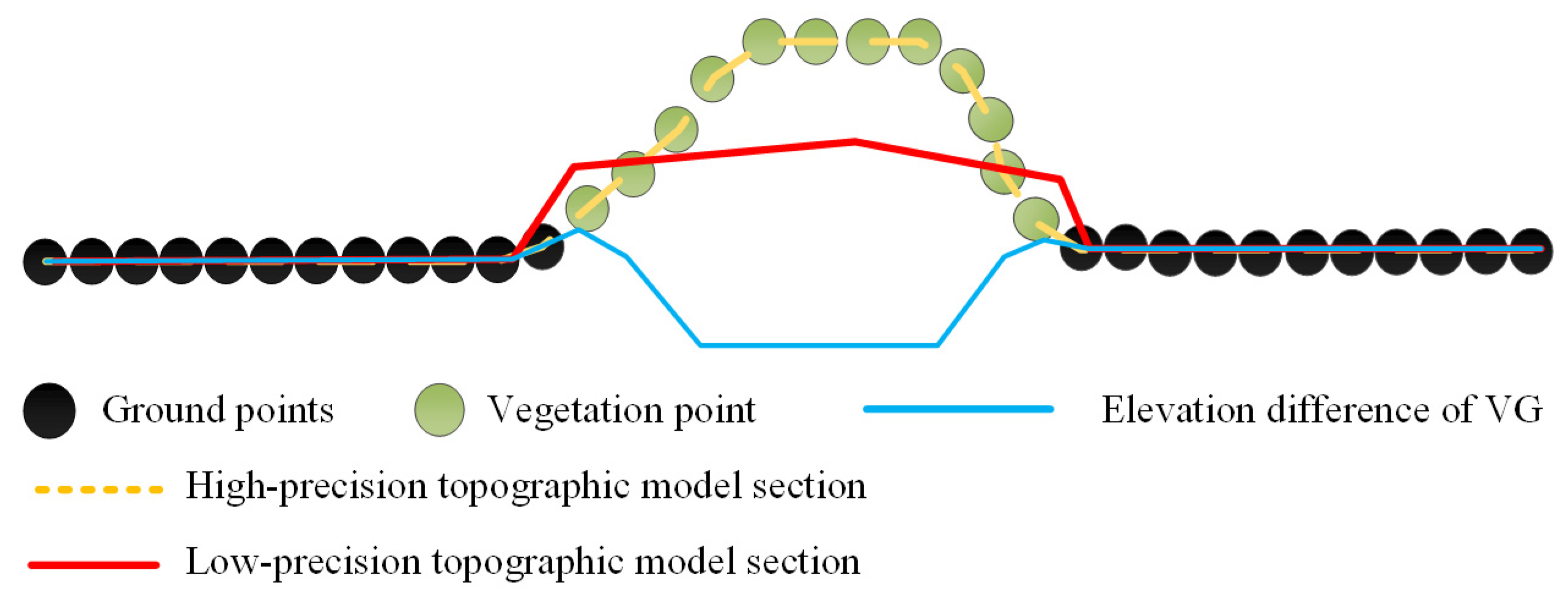
2.3. Elevation Differences

The spatial scale of a VG directly impacts the corresponding data volume and representation accuracy, as well as the calculation of topographic factors such as the elevation variation coefficient, slope, and slope direction. Different spatial scales of VGs encompass different topographic and geomorphological features. As the spatial scale of a VG increases, the accuracy of the description of surface details is gradually smoothed, and the features are gradually integrated. In contrast, as the spatial scale of the VG becomes finer, the description of surface details gradually increases, and the smaller the spatial scale is, the more accurately and realistically the detailed features of the surface within the region are reflected. Therefore, calculating the elevation differences of VGs at different spatial scales can reflect discrepancies in the surface features contained in VGs at different scales (e.g., vegetation). As shown in Figure 3, the black points represent the ground points, and the green points represent the vegetation points. A high-precision topographic model generated from a small-scale VG provides high precision for describing surface details. A low-precision topographic model generated with a large-scale VG provides a rough representation of surface details, and surface features tend to be flat. The elevation difference among VGs at different spatial scales can be calculated, and significant fluctuations often appear at the edges of vegetation points. Because of the different sizes of VGs, an output standard is required when calculating the differences between two VGs. We chose a small VG as the output standard. To obtain the optimal parameters, VG thresholds ranging from 0.1 to 3.2 m were considered.

2.4. Multiscale Coefficients of Elevation Variation

The elevation variation coefficient (EVC) is an important terrain factor in digital terrain analysis. As a variable that reflects the dispersion degree of the average elevation, it is the ratio of the standard deviation and average of the elevations at different points, which can reflect differences in terrain characteristics. The corresponding calculation is shown in Formula (1). The EVC can directly represent the variations in elevation in different-scale VGs and minimize the effect of noise.
E V C = H s t d / H m e a n
where EVC is the elevation variation coefficient of a VG in the analysis area, which objectively reflects differences in elevation in the analysis area. Hstd is the standard deviation of elevation in the VG statistical window, and Hmean is the mean elevation in the VG statistical window.
To calculate the standard deviation and mean of elevation in each VG statistical window, elevation differences are determined in neighborhoods, and the result for a neighborhood grid is used as the new value of the central grid. The multiscale VG statistical windows are shown in Figure 4. To obtain the optimal parameters, thresholds of 1–6 grid were considered.

2.5. Accuracy Assessment

We manually classified the ground and vegetation points as reference data. The results of the proposed method were then compared with the reference data. To evaluate the accuracy of terrain modeling, we used the method recommended by the International Society for Photogrammetry and Remote Sensing (ISPRS) for quantitative analysis [30]. The method proposed by the ISPRS in 2003 is shown in Table 1. The precision of the vegetation removal results was quantified and evaluated based on type I error, type II error, and total error.
In Table 1, a represents the number of ground points correctly classified as ground points. b represents the number of ground points incorrectly classified as vegetation points (affecting type I error). c represents the number of vegetation points incorrectly classified as ground points (affecting type II error). d represents the number of vegetation points correctly classified as vegetation points. Additionally, e represents the number of ground points in the reference dataset used for visual interpretation classification. f represents the number of vegetation points in the reference dataset used for visual interpretation classification. g represents the number of ground points used in terrain modeling. h represents the number of feature points used in terrain modeling. n represents the total number of point clouds.
Three indices were calculated for accuracy assessment. Type I error represents the proportion of ground points that were incorrectly classified as vegetation points, also known as truth-rejection errors. Type II error represents the proportion of vegetation points that were incorrectly classified as ground points, also known as false-tolerance errors. Total error represents the overall error proportion, which reflects the inconsistency between terrain modeling results and actual values. The corresponding formulas are as follows.
Type   I   error = b e × 100 %
Type   II   error = c f × 100 %
Total   error = b + c n × 100 %

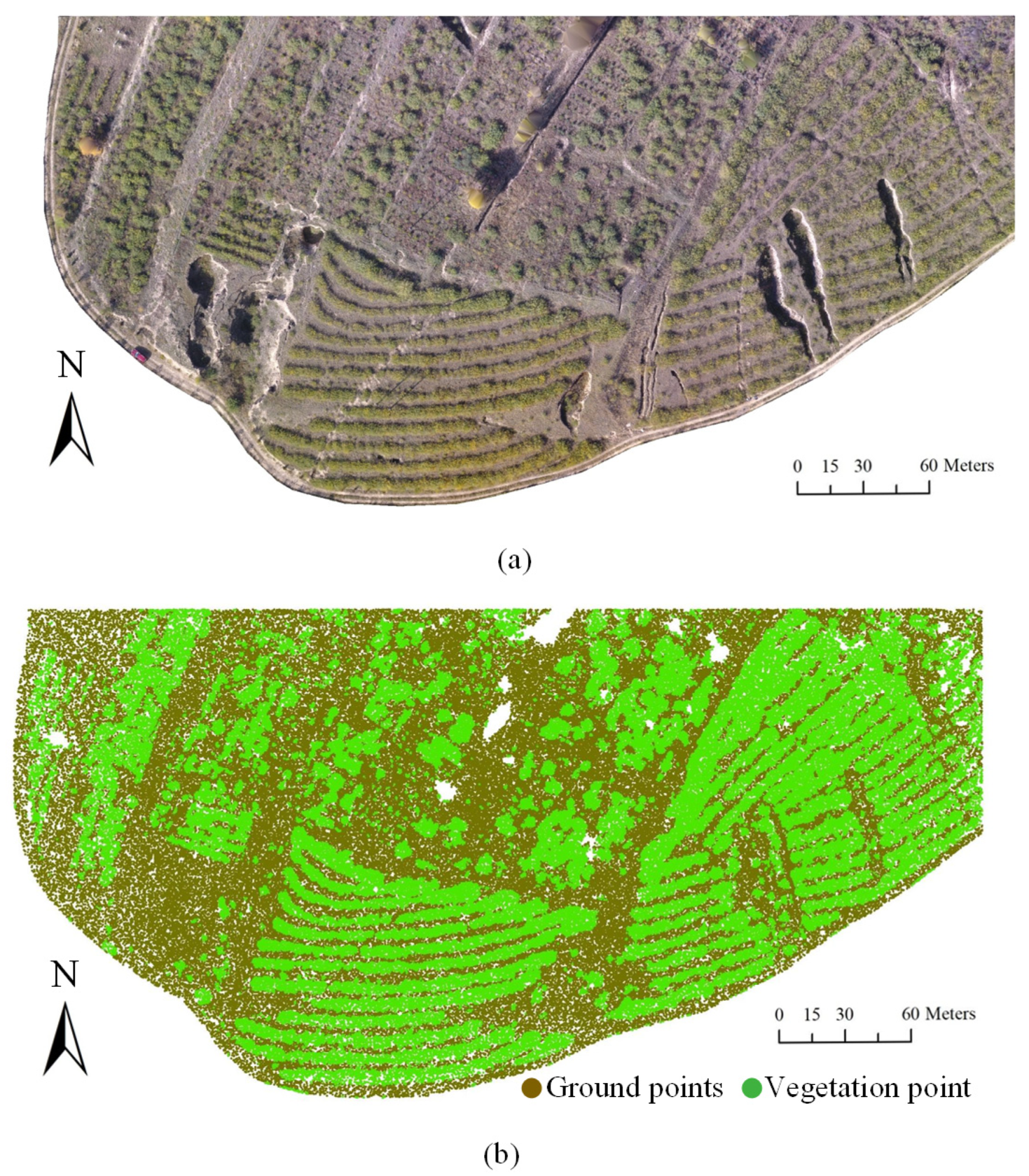
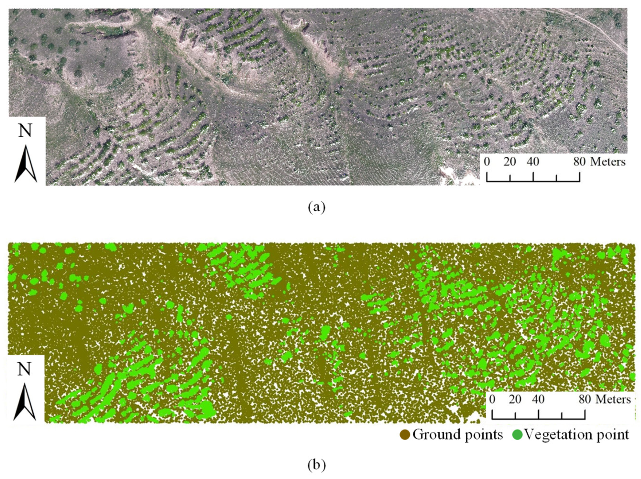
2.6. Study Areas and Data
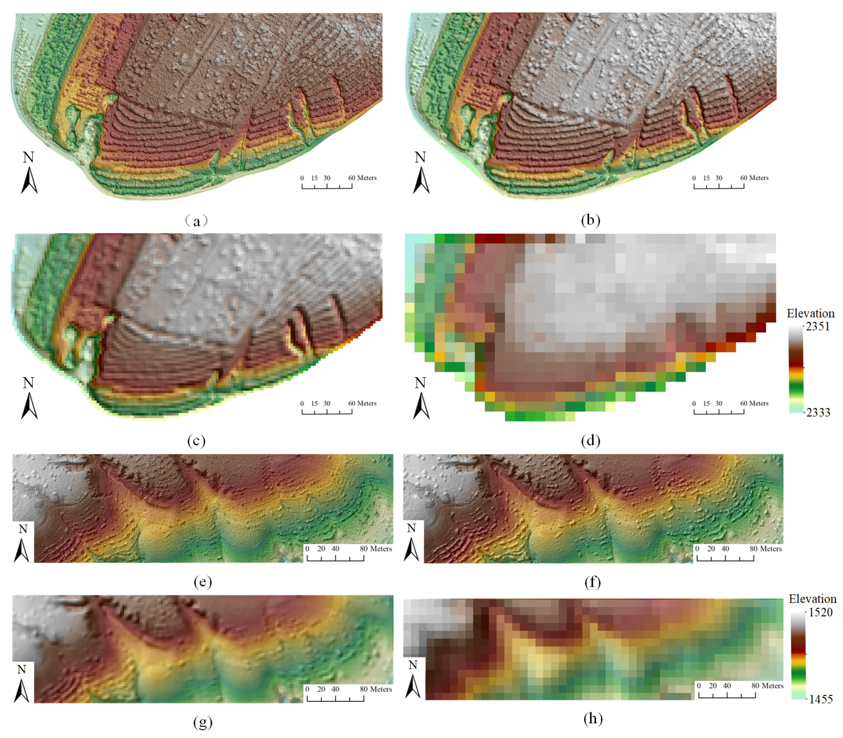
Two study areas (T1 and T2) were used to validate the proposed method. The T1 area was located in Xining city, Qinghai Province, China. A Da-Jiang Inspire1 UAV equipped with a 20 mm fixed-focus lens and PIX4Dmapper 4.7.5 software were used to perform image matching, aerial triangulation, and dense point-cloud matching. The study area was flanked by steep cliffs to the south, and the quality of the point cloud was poor in this area. Therefore, the study area was cropped using the main southern road as the boundary. The study area covered 23,439.46 square meters. The point density was 189 points/m2. In addition to ground points, the study area contained a large amount of vegetation and a small number of man-made ground objects. The vegetation mainly included two types of dense low vegetation, which were connected in strips in some areas and isolated in others. The orthophoto image and reference cloud points for T1 are shown in Figure 5. The T2 area was located in Yulin city, Shaanxi Province, China. UAVs were used to collect data and produce aerial images of Madigou. The study area covered 28,881.2 square meters. The point density was 27 points/m2. This area contained a large amount of vegetation. The vegetation was mainly isolated as single points, with a small amount of densely aggregated vegetation. The orthophoto image and reference cloud points for T2 are shown in Figure 6. Field research and expert visual interpretation were used to select the reference data.

3. Results

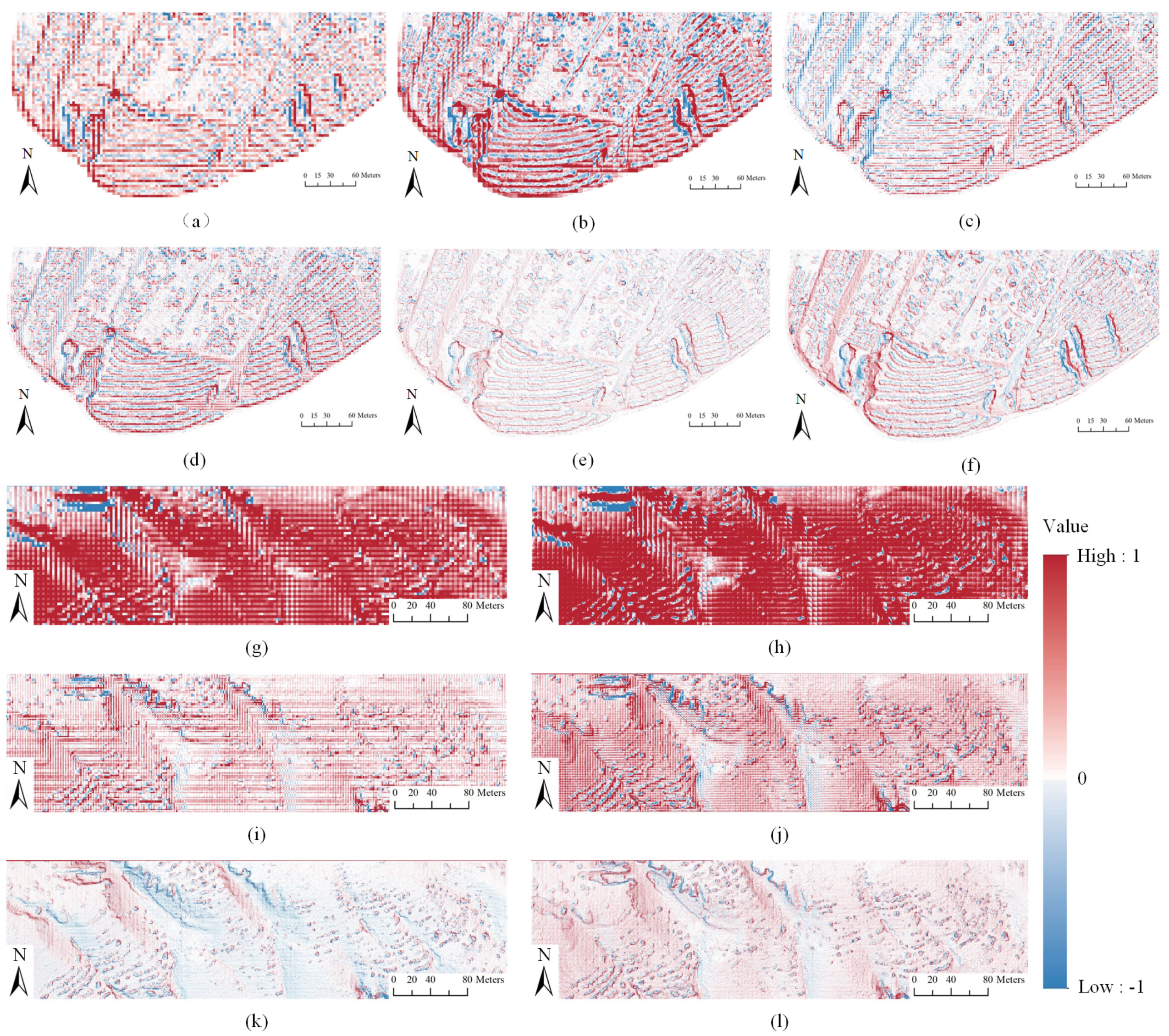
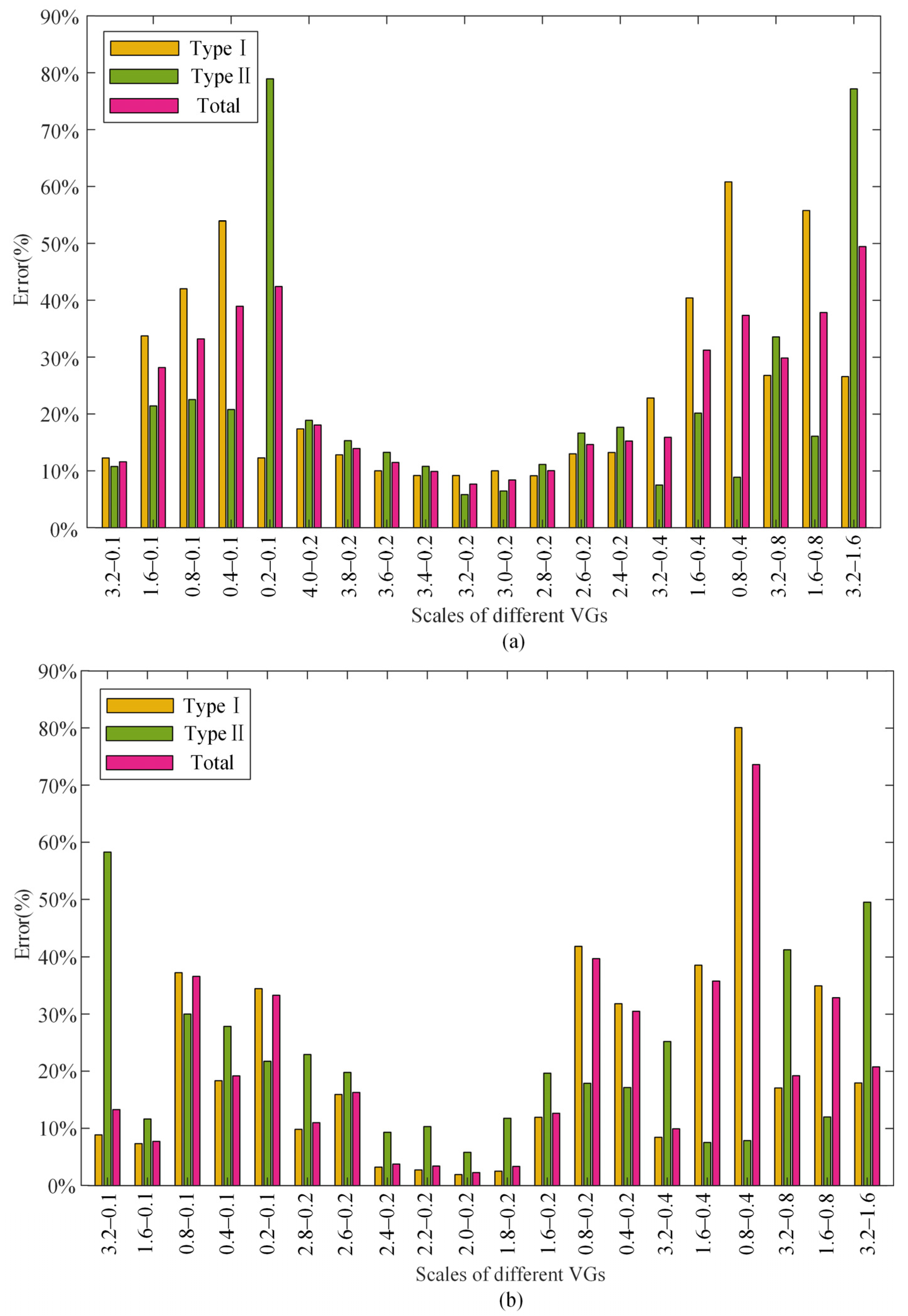
3.1. Optimal Scale of the Virtual Grid

Figure 7 shows the digital surface model generated for the study area at different VG scales. The surface features vary at different scales. In the small-scale VG, the surface details are obvious, and low vegetation can be clearly expressed. In the 6.4 m VG, only abrupt surface features such as gullies and steep slopes can be observed, and the surface vegetation features are basically smoothed. In VGs with a scale greater than 6.4 m, small-scale surface features can no longer be observed.
Figure 8 shows the results of the elevation variations in VGs at different scales in the study area. The scale of the output result is equal to that of the small-scale grid when calculating the elevation change. The VGs can no longer express the surface features with scales larger than 6.4 m, so scales larger than 6.4 m were not considered when selecting the VG scale.
The elevation variations between pairs of VG scales highlight the areas with abrupt changes in the surface in the sample area. To obtain the best VG scale, quantitative comparisons and analyses were performed based on the terrain modeling error results for the different elevation variations shown above. In the process of terrain modeling, the neighborhood radius and segmentation threshold were selected as constants in all cases. The neighborhood radius was selected as a pixel unit, and the segmentation threshold was determined using the natural breakpoint method. The thresholds of point-cloud filtering are shown in Table 2. The ground feature points included the vegetation area and vegetation boundaries. The threshold value of the vegetation area was (−∞,0], the threshold value of vegetation boundaries was (1.5,+∞), and the threshold value of ground points was (0,1.5]. After threshold segmentation, the attributes of ground points and vegetation points were assigned to the point cloud in the corresponding virtual grid to remove the surface vegetation and improve the accuracy of terrain modeling. A comparison of error results is shown in Figure 9.
As shown in Figure 8 and Figure 9, the contrast between ground points and vegetation points is gradually enhanced with increasing grid-scale difference. The larger the scale difference is, the more prominent the vegetation characteristics are. Vegetation tends to be difficult to identify in areas with considerable elevation variation. The smaller the scale difference is, the higher the similarity between the top of vegetation and the ground. The variation trends for the type I error, type II error, and total error were different at different scales. As the VG scale gap increased, the three kinds of errors generally displayed downward trends. The error in the elevation variation results obtained at the 3.2 m and 1.6 m scales was the largest because the output scale at 1.6 m could not express terrain features well, resulting in a large number of errors. The error decreased when 0.2 m was used as the small-scale VG. Figure 9a indicates that type I error was the smallest among the error results for elevation variations between the 3.2 m and 0.2 m scales, followed by that between the 2.8 m and 0.2 m scales. The final terrain modeling result based on the difference between grids at 3.2 m and 0.2 m scales was associated with the smallest type II error, followed by that between the results at the 3.0 m and 0.2 m scales. The total error was lowest based on the difference between the 3.2 m and 0.2 m scales, followed by that between 3.0 m and 0.2 m. Based on the three types of errors, 0.2 m was the VG scale that yielded the smallest error for T1. Figure 9b indicates that type I error was the smallest among the error results for elevation variations between the 1.8 m and 0.2 m scales, followed by that between the 2.2 m and 0.2 m scales. The final terrain modeling result based on the difference between grids at 2.0 m and 0.2 m scales was associated with the smallest type II error, followed by that between the results at the 0.8 m and 0.4 m scales. The total error was lowest based on the difference between the 2.0 m and 0.2 m scales, followed by that between 1.8 m and 0.2 m. Based on the three types of errors, 0.2 m was the VG scale that yielded the smallest error for T2. The results indicate that it is possible to not only avoid misjudgments caused by a low output resolution, but also to avoid the increased noise associated with a high output resolution. Finally, the 3.2 m and 0.2 m scales of VGs of T1 and the 2.0 m and 0.2 m scales of VGs of T2 were selected to continue the multiscale neighborhood calculation of EVCs to determine the best-scaled neighborhoods.

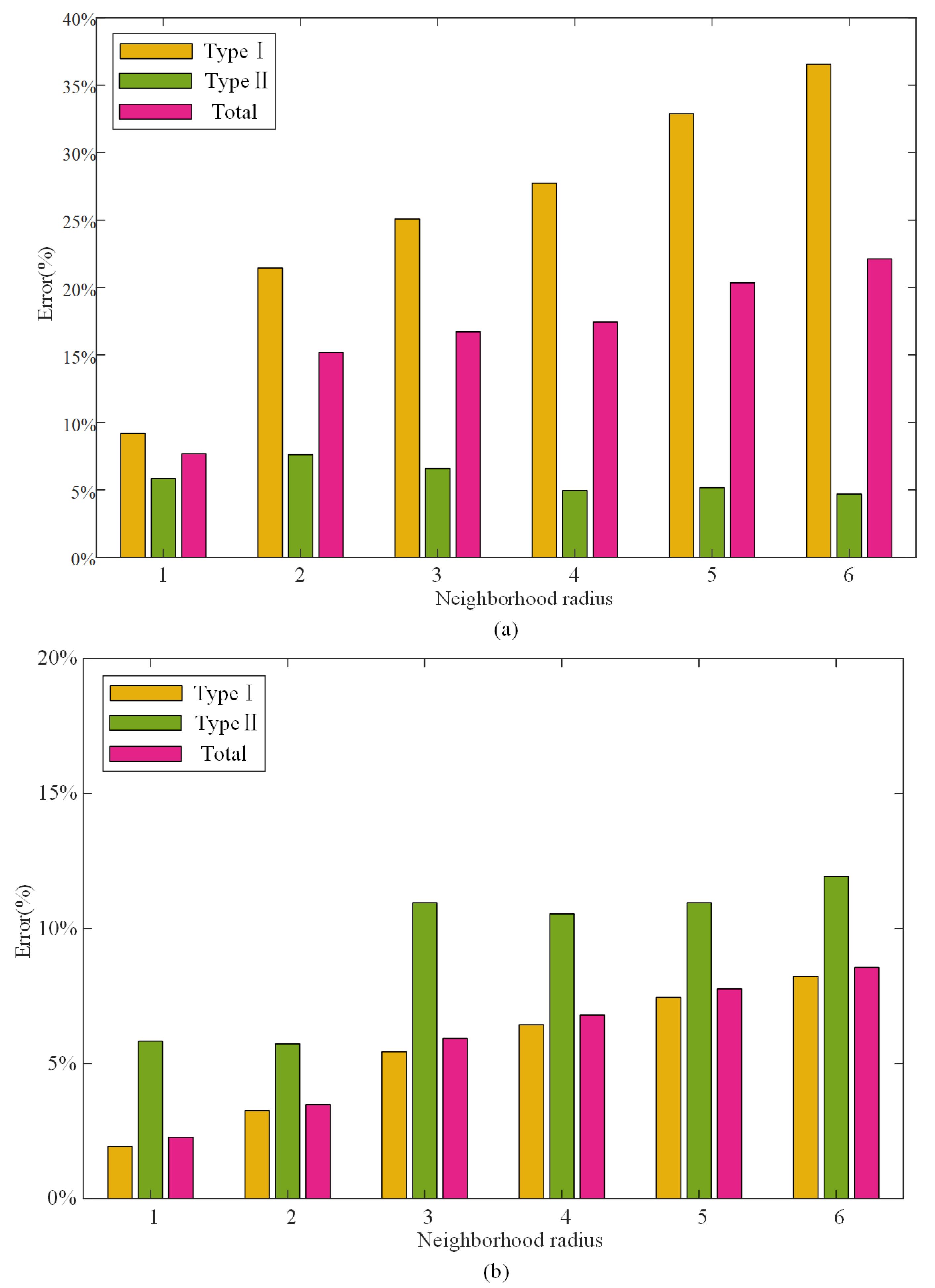
3.2. Optimal Neighborhood Radius

Figure 10 shows the results of EVCs obtained under different neighborhood radii for 3.2 m and 0.2 m elevation variations for T1 and 2.0 m and 0.2 m elevation variations for T2. The ground points displayed obvious false negatives after the neighborhood radius reached 6 VG radius. Therefore, only the EVCs in a neighborhood radius of 1–6 VGs were analyzed.
Figure 10 shows that the areas with negative values correspond to vegetation, and the boundaries around vegetation are highlighted. The vegetation boundaries become more prominent and the contrast between ground and vegetation becomes more prominent with increasing neighborhood radius. However, the vegetation areas display obvious false negatives inside boundaries in some cases, and low and small vegetation areas also correspond to false negatives.
The error results for terrain modeling with different-scale EVCs were quantitatively compared and analyzed. The same threshold was selected for segmentation in the process of terrain modeling. The trends of the type I error and total error are the same in the quantitative error comparison in Figure 11. The error increased with increasing scale. The error decreased with increasing scale for the type II error in T1 in Figure 11a, but the range of change was small. The error increased with increasing scale for the type II error in T1 in Figure 11b. Based on the results in Figure 10 and Figure 11, it can be concluded that the filtering result obtained by calculating the EVC in a one-neighborhood radius was the most accurate.

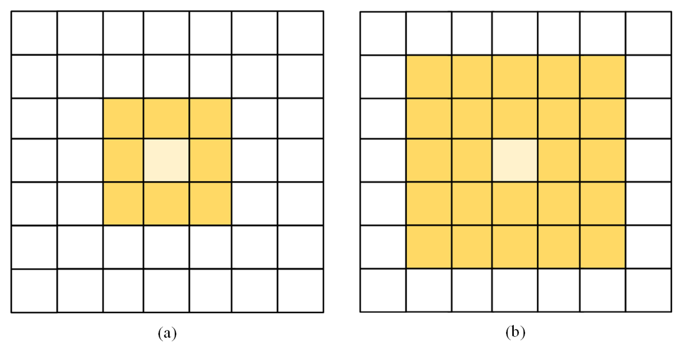
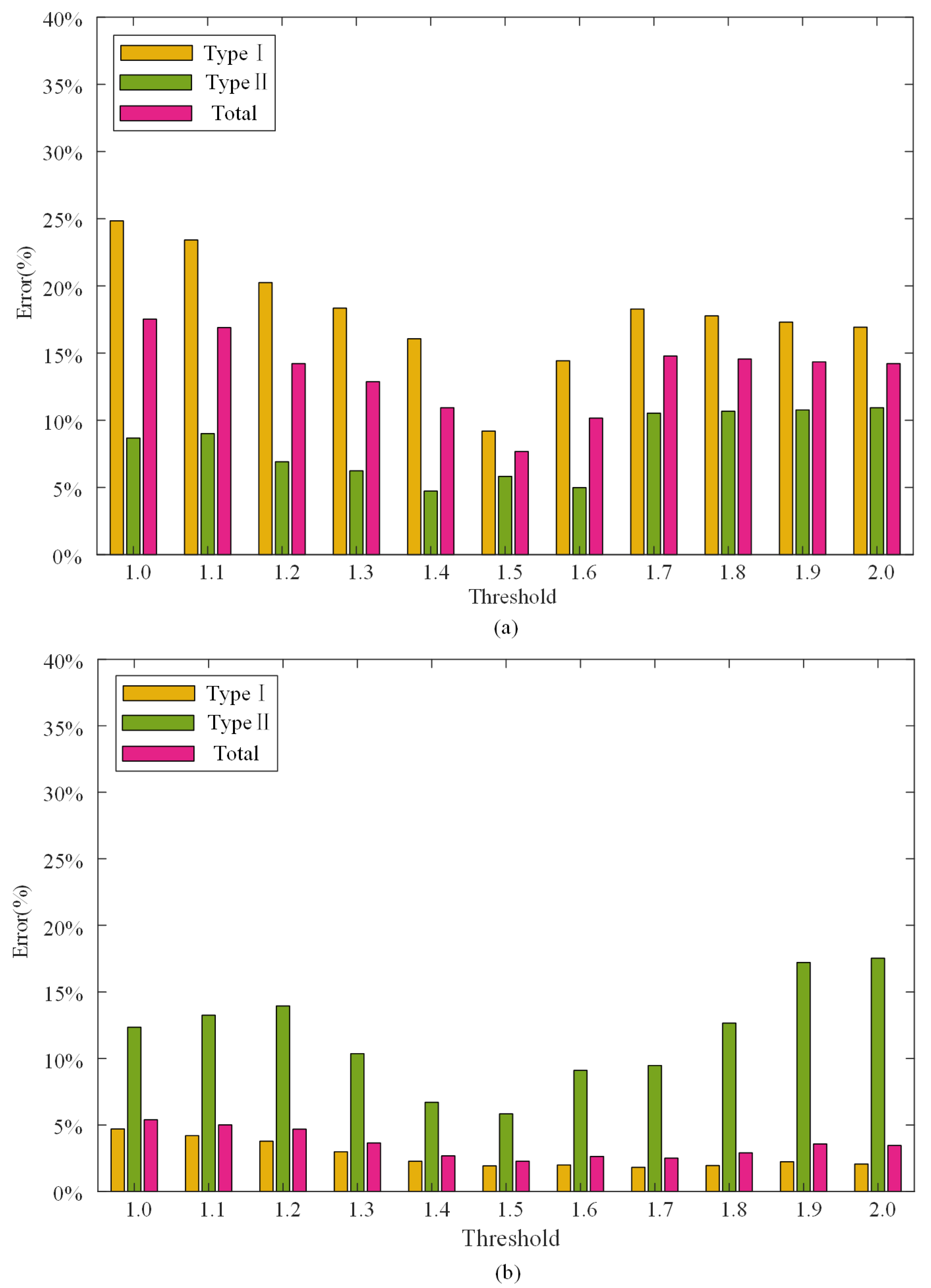
3.3. Optimal Segmentation Threshold

The optimal threshold value was selected based on the results of the optimal scale elevation-variation coefficient. The error at different thresholds was analyzed and quantitatively assessed by comparing the terrain modeling results for the 3.2 m and 0.2 m EVCs in one-pixel neighborhoods. The values in vegetation areas were mostly negative after calculating the elevation variation in the VGs at different scales, and the corresponding EVCs were also negative. The selection of the threshold was mainly affected by vegetation boundaries. A comparison of the filtering error results is shown in Figure 12.
It is obvious from the quantitative error comparison in Figure 12 that the variation in the error was related to the selection of threshold. The trends of the type I error and total error were roughly the same. As the segmentation threshold decreased from 1.0 to 1.5, minimum error was observed at 1.5. Then, as the threshold increased from 1.5 to 2.0, the error continually increased. The overall variation trend was the same for the type II error, with a minimum error at a threshold of 1.4, followed by 1.6 and 1.5. After comprehensive consideration, the terrain modeling accuracy was the highest when the segmentation threshold was 1.5. In the experiment, it was found that the segmentation threshold displayed a certain relationship with the vegetation height in the sample area. The abrupt changes in vegetation edges were the most obvious, and the EVC increased with increasing vegetation height.

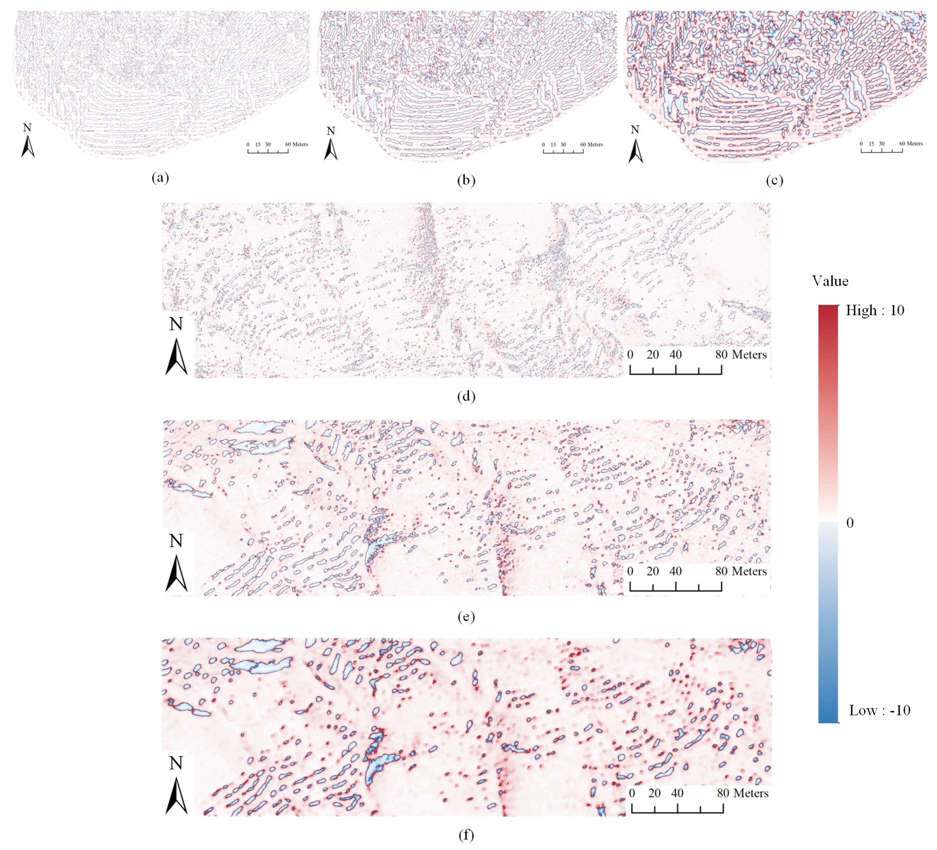
3.4. Accuracy Analysis

The terrain-modeling method based on the EVC was applied in two research areas to evaluate the accuracy of the method. The specific parameter selection scheme was analyzed in detail using the T1 area as an example, and the same approach was used for T2. Table 3 shows the parameters used in the experiment in the two study areas.
The error results based on the test data are shown in Table 4. The type I error, type II error, and total error in the T1 area were 9.20%, 5.83%, and 7.68%, respectively. The type I error, type II error, and total error in the T2 area were 1.93%, 5.84%, and 2.28%, respectively. The type I error was larger than the type II error, which was due to the large amount of vegetation-covered areas in the study area. The purpose of point-cloud filtering is to accurately extract ground points and ensure terrain accuracy. Therefore, type II errors should be controlled first. Some type I errors could be sacrificed to ensure that the filtered data do not contain areas of vegetation.

4. Discussion

The accuracy of terrain modeling based on UAVs is significantly affected by surface vegetation [31]. Therefore, vegetation removal is an important step in terrain modeling. Accurate vegetation removal is the key to ensuring the accuracy of terrain models. The current methods have shortcomings in areas with complex terrain and low vegetation, and they mainly identify and remove vegetation based on specific scales [32]. However, the characteristics of terrain and ground features at different spatial scales are obviously different, and it is difficult to accurately distinguish vegetation by only considering the characteristics of a single scale [33]. Some scholars have improved modeling methods from the perspective of multiscale progression [26,34,35], but individual features are extracted.
In recent years, point-cloud filtering methods based on deep learning have gradually increased in popularity [36,37]. In these methods, the point clouds of training samples are usually labeled with different categories. Not only ground points and vegetation points, but also multiple classes of objects such as trees, roads, and buildings can be detected. These methods represent a new research direction. However, the implementation of these methods requires a large number of samples to be labeled and trained in advance. The characteristics of training samples and the accuracy of labeling have a considerable impact on the final results.
In this approach, a series of variations in elevation values after scale synthesis based on VGs reflect the characteristics of the terrain at different scales. Therefore, a UAV terrain-modeling method based on multiscale EVCs in low-vegetation areas is proposed using elevation variability coefficients to quantify and extract differences in topographic features at different scales.
To measure the final terrain-modeling accuracy of this method, cloth simulation filtering (CSF), triangulated irregular network (TIN) filtering, and progressive morphological filtering (PMF) were used to model the terrain in the two study areas. The parameter settings of the three methods referred to the references [6,8,38] to optimize their filtering results and, thus, the comparison with our method is reasonable. These three methods were implemented in the software packages CloudCompare, Photoscan, and PCL, respectively. The point cloud after vegetation removal with our method is shown in Figure 13a. The parameters of compared methods were set as follows. In the CSF method, the scene was set to steep slope, the cloth resolution was set to 0.3, the maximum number of iterations was set to 500, the classification threshold was set to 0.2, and the slope preprocessing condition was set to off. The point cloud after vegetation removal with the CSF method is shown in Figure 13b. Notably, vegetation removal was most effective in areas of dense vegetation cover, but less effective in gully areas with complex topography. In the TIN method, the max angle was set to 10, the max distance was set to 0.5, and the cell size was set to five. The point cloud after vegetation removal with the TIN method is shown in Figure 13c. Topographic features were preserved in gully areas, but the method performed poorly in areas of dense vegetation cover. In the PMF method, the max window size was set to five, the terrain slope was set to 0.5 f, the initial elevation threshold was set to 0.5 f, and the max elevation threshold was set to 0.5 f. The point cloud after vegetation removal with the PMF method is shown in Figure 13d. The method was effective in filtering and removing vegetation in flat areas, but performed poorly in areas of dense vegetation cover and areas with gullies. The DEM obtained by interpolating the point-cloud data after vegetation removal with our method for the T1 area is shown in Figure 13f.
The point cloud after vegetation removal with our method is shown in Figure 14a. The parameters of the compared methods were set as follows. In the CSF method, the scene was set to steep slope, the cloth resolution was set to 0.3, the maximum number of iterations was set to 500, the classification threshold was set to 0.3, and the slope preprocessing condition was set to on. The point cloud after vegetation removal with the CSF method is shown in Figure 14b. In the TIN method, the max angle was set to 0.3, the max distance was set to 0.5, and the cell size was set to one. The point cloud after vegetation removal with the TIN method is shown in Figure 14c. In the PMF method, the max window size was set to three, the terrain slope was set to 0.5 f, the initial elevation threshold was set to 0.5 f, and the max elevation threshold was set to 0.5 f. The point cloud after vegetation removal with the PMF method is shown in Figure 14d. The DEM obtained by interpolating the point cloud after vegetation removal with our method for the T2 area is shown in Figure 14f.
Figure 13a and Figure 14a show that the proposed filtering algorithm can effectively filter the ground points and effectively remove a large amount of vegetation cover. Compared with the other methods, it can better deal with areas with low vegetation coverage and preserve the details of terrain. A comparison of Figure 13f and Figure 14f with Figure 13e and Figure 14e indicates that compared with the DSM, the DEM retains the topographic features of the region and effectively eliminates vegetation points. A comparison of Figure 13a–d and Figure 14a–d indicates that CSF can be used to remove most of the vegetation, but the effect is poor for low vegetation distributed in patches, and the terrain boundaries are eliminated where the slope changes greatly. The TIN method preserves the boundaries of terrain, but the effect of vegetation removal is poor in areas with large terrain gradients. The PMF method works well in flat-terrain areas, but it does not work well in some areas with large topographic relief, and the algorithm has many parameters that are difficult to set. We quantitatively analyzed the results of the different methods, and an error comparison is shown in Table 5.
The results in Table 5 show that the method based on the multiscale EVC is superior to the CSF, TIN, and PMF methods in terms of the type I error, type II error, and total error based on the terrain-modeling results for the T1 and T2 study areas. In general, the filtering algorithm proposed in this study is more suitable for areas with low and dense vegetation. Notably, low vegetation is filtered, and the ground points are accurately retrained, thus meeting the requirements for generating high-precision DEMs.
The point-cloud densities in the two study areas differ significantly at 189 points/m2 and 27 points/m2, respectively. However, the parameter settings for the two study areas are almost identical, except for the large-scale VG. The point-cloud density may affect the results. If the point cloud is too sparse, the optimal scale may be difficult to determine because the sparse point cloud will not include all the vegetation or terrain relief information. However, in this study, the point-cloud densities were all sufficiently high, so the result varied little with the selected threshold. In addition, although the point-cloud density varied, the vegetation type (low-rise vegetation), and topography in the two plots were similar, and, thus, the threshold values were also similar. This indicates that the effect of vegetation type may be greater than that of the point-cloud density. In addition, the optimal size of the small-scale VG in both study areas was 0.2 m. The size of the small-scale VG determined the size of the output elevation difference. The size of 0.2 m not only ensures the precision of vegetation removal but also avoids misjudgments regarding areas of low topographic relief. The optimal value of the neighborhood radius for both sample areas was one grid. Increasing the neighborhood radius does not have a significant effect on the type II error and mainly causes rapid increases in the type I error and the total error (the proportion of ground points misclassified as vegetation points increases). To ensure accuracy, the optimal solution for the neighborhood radius should be re-explored based on the study area. The vegetation in both study areas was characterized by low-growing vegetation. The optimal solution for the splitting threshold in both study areas was 1.5. This value ensures that the vast majority of low vegetation in both study areas can be identified. The optimal size of the large-scale VG varied in the two study areas. The optimal value for T1 was 3.2 m, but the optimal value for T2 was 2.0 m. The vegetation in T1 was densely distributed, and the vegetation in T2 was characterized by a mostly isolated distribution. Vegetation distribution patterns may be related to the appropriate selection of the size of the large-scale VG. In future work, the applicability of the methods in this paper can be verified in areas with high vegetation coverage or containing artificial features. However, the choice of parameters may not yield the same results. Future improvements to this method in terms of the adaptive selection of parameters should be considered. Furthermore, UVA photogrammetry can obtain optical images of the test areas, and the normalized difference vegetation index (NDVI) can be used to identify vegetated areas. Notably, the NDVI could be introduced in follow-up research to improve the filtering accuracy.

5. Conclusions

This paper addresses the issue of vegetation removal during terrain modeling. According to the different topographic features expressed by point-cloud data at different scales, a terrain-modeling method based on multiscale EVCs was proposed in this paper. The amount of elevation change between any two different scales of VGs was calculated and the EVC of the VG that yielded the largest elevation variation was determined. The optimal parameters were analyzed and discussed. The experimental results show that the multiscale EVC method can accurately remove vegetation points and reserve ground points in low and dense vegetation-covered areas. The error results were better than those of the CSF, TIN, and PMF methods. The type I error, type II error, and total error in the study areas ranged from 1.93 to 9.20%, 5.83 to 5.84%, and 2.28 to 7.68%, respectively. The total error of the proposed method was 2.43–2.54% lower than that of the CSF, TIN, and PMF algorithms in the study areas.
The parameters of the proposed method are easier to set than those of other methods. The parameters minimally changed between the two study areas. The optimal small-scale VG, neighborhood radius, and threshold in the two study areas were the same (0.2 m for the small-scale VG, 1 grid for the optimal neighborhood radius, and 1.5 for the threshold), thus highlighting the robustness of the proposed method. Only the large-scale VG changed in the two study areas. The larger the scale difference is, the more prominent the vegetation characteristics are. The optimal large-scale VG size was 3.2 m in the T1 and 2.0 m at T2, which is only a minor difference. The optimal scale of VGs may differ in different areas, and this scale is related to vegetation distribution patterns. In general, we recommend 2.0–3.0 m as the large-scale VG size. The proposed method provides a foundation for the rapid establishment of high-precision DEMs based on UAV photogrammetry.

Author Contributions

Conceptualization, J.F. and W.D.; methodology, J.F. and W.D.; software, J.F.; validation, J.F., W.D. and B.W.; formal analysis, J.Y.; investigation, K.C.; resources, B.W.; data curation, J.F.; writing—original draft preparation, J.F.; writing—review and editing, W.D.; visualization, J.L.; supervision, W.D.; project administration, B.W.; funding acquisition, J.F and B.W. All authors have read and agreed to the published version of the manuscript.

Funding

We are grateful for the financial support provided by the Natural Science Foundation of the Jiangsu Higher Education Institutions of China (No. 22KJB170016), the National Natural Science Foundation of China (No. 42171402 and 41930102), and the Graduate Practice Innovation Program of the Jiangsu Province of China (No. SJCX23_0418).

Data Availability Statement

Not applicable.

Conflicts of Interest

The authors declare no conflict of interest.

References

  1. Shahbazi, M.; Menard, P.; Sohn, G.; Théau, J. Unmanned aerial image dataset: Ready for 3D reconstruction. Data Brief 2019, 25, 103962. [Google Scholar] [CrossRef] [PubMed]
  2. Berrett, B.E.; Vernon, C.A.; Beckstrand, H.; Pollei, M.; Markert, K.; Franke, K.W.; Hedengren, J.D. Large-scale reality modeling of a university campus using combined UAV and terrestrial photogrammetry for historical preservation and practical use. Drones 2021, 5, 136. [Google Scholar] [CrossRef]
  3. Dai, W.; Qian, W.; Liu, A.; Wang, C.; Yang, X.; Hu, G.; Tang, G. Monitoring and modeling sediment transport in space in small loess catchments using UAV-SfM photogrammetry. CATENA 2022, 214, 106244. [Google Scholar] [CrossRef]
  4. Dai, W.; Tang, G.; Hu, G.; Yang, X.; Xiong, L.; Wang, L. Modelling sediment transport in space in a watershed based on topographic change detection by UAV survey. Prog. Geogr. 2021, 40, 1570–1580. [Google Scholar] [CrossRef]
  5. Meng, X.; Currit, N.; Zhao, K. Ground filtering algorithms for airborne LiDAR data: A review of critical issues. Remote Sens. 2010, 2, 833–860. [Google Scholar] [CrossRef] [Green Version]
  6. Axelsson, P. DEM generation from laser scanner data using adaptive TIN models. Int. Arch. Photogramm. Remote Sens. 2000, 33, 110–117. [Google Scholar]
  7. Yang, Y.B.; Zhang, N.N.; Li, X.L. Adaptive slope filtering for airborne Light Detection and Ranging data in urban areas based on region growing rule. Emp. Surv. Rev. 2016, 49, 139–146. [Google Scholar] [CrossRef]
  8. Zhang, W.; Qi, J.; Wan, P.; Wang, H.; Yan, G. An Easy-to-Use Airborne LiDAR Data Filtering Method Based on Cloth Simulation. Remote Sens. 2016, 8, 501. [Google Scholar] [CrossRef]
  9. Dong, Y.; Cui, X.; Zhang, L.; Ai, H. An Improved Progressive TIN Densification Filtering Method Considering the Density and Standard Variance of Point Clouds. Int. J. Geo-Inf. 2018, 7, 409. [Google Scholar] [CrossRef] [Green Version]
  10. Véga, C.; Durrieu, S.; Morel, J.; Allouis, T. A sequential iterative dual-filter for Lidar terrain modeling optimized for complex forested environments. Comput. Geosci. 2012, 44, 31–41. [Google Scholar] [CrossRef]
  11. Hui, Z.; Jin, S.; Xia, Y.; Nie, Y.; Li, N. A mean shift segmentation morphological filter for airborne LiDAR DTM extraction under forest canopy. Opt. Laser Technol. 2021, 136, 106728. [Google Scholar] [CrossRef]
  12. Chen, Q.; Gong, P.; Baldocchi, D.; Xie, G. Filtering airborne laser scanning data with morphological methods. Photogramm. Eng. Remote Sens. 2007, 73, 175. [Google Scholar] [CrossRef] [Green Version]
  13. Huang, S.; Liu, L.; Dong, J.; Fu, X.; Huang, F. SPGCN: Ground filtering method based on superpoint graph convolution neural network for vehicle LiDAR. J. Appl. Remote Sens. 2022, 16, 016512. [Google Scholar] [CrossRef]
  14. Yilmaz, V. Automated ground filtering of LiDAR and UAS point clouds with metaheuristics. Opt. Laser Technol. 2021, 138, 106890. [Google Scholar] [CrossRef]
  15. Sithole, G. Filtering of Laser Altimetry Data using a Slope Adaptive Filter. Int. Arch. Photogramm. Remote Sens. 2011, 34, 203–210. [Google Scholar]
  16. Chen, C.; Chang, B.; Li, Y.; Shi, B. Filtering airborne LiDAR point clouds based on a scale-irrelevant and terrain-adaptive approach. Measurement 2021, 171, 108756. [Google Scholar] [CrossRef]
  17. Xia, T.; Yang, J.; Chen, L. Automated semantic segmentation of bridge point cloud based on local descriptor and machine learning. Autom. Constr. 2022, 133, 103992. [Google Scholar] [CrossRef]
  18. Chen, C.; Guo, J.; Wu, H.; Li, Y.; Shi, B. Performance comparison of filtering algorithms for high-density airborne Lidar point clouds over complex landscapes. Remote Sens. 2021, 13, 2663. [Google Scholar] [CrossRef]
  19. Kláptě, P.; Fogl, M.; Barták, V.; Gdulová, K.; Urban, R.; Moudr, V. Sensitivity analysis of parameters and contrasting performance of ground filtering algorithms with UAV photogrammetry-based and LiDAR point clouds. Int. J. Digit. Earth 2020, 13, 23. [Google Scholar] [CrossRef]
  20. Li, H.; Ye, W.; Liu, J.; Tan, W.; Pirasteh, S.; Fatholahi, S.N.; Li, J. High-resolution terrain modeling using airborne lidar data with transfer learning. Remote Sens. 2021, 13, 3448. [Google Scholar] [CrossRef]
  21. Dai, W.; Yang, X.; Na, J.; Li, J.; Brus, D.; Xiong, L.; Tang, G.; Huang, X. Effects of DEM resolution on the accuracy of gully maps in loess hilly areas. CATENA 2019, 177, 114–125. [Google Scholar] [CrossRef]
  22. Li, S.; Dai, W.; Xiong, L.; Tang, G. Uncertainty of the morphological feature expression of loess erosional gully affected by DEM resolution. J. Geo-Inf. Sci. 2020, 22, 338–350. [Google Scholar]
  23. Xiong, L.; Li, S.; Tang, G.; Strobl, J. Geomorphometry and terrain analysis: Data, methods, platforms and applications. Earth-Sci. Rev. 2022, 233, 104191. [Google Scholar] [CrossRef]
  24. Cai, S.; Liang, X.; Yu, S. A Progressive Plane Detection Filtering Method for Airborne LiDAR Data in Forested Landscapes. Forests 2023, 14, 498. [Google Scholar] [CrossRef]
  25. Song, D. A Filtering Method for LiDAR Point Cloud Based on Multi-Scale CNN with Attention Mechanism. Remote Sens. 2022, 14, 6170. [Google Scholar]
  26. Hui, Z.; Hu, Y.; Yevenyo, Y.Z.; Yu, X. An Improved Morphological Algorithm for Filtering Airborne LiDAR Point Cloud Based on Multi-Level Kriging Interpolation. Remote Sens. 2016, 8, 35. [Google Scholar] [CrossRef] [Green Version]
  27. Bailey, G.; Li, Y.; McKinney, N.; Yoder, D.; Wright, W.; Herrero, H. Comparison of Ground Point Filtering Algorithms for High-Density Point Clouds Collected by Terrestrial LiDAR. Remote Sens. 2022, 14, 4776. [Google Scholar] [CrossRef]
  28. Hiep, N.H.; Luong, N.D.; Ni, C.F.; Hieu, B.T.; Huong, N.L.; Duong, B.D. Factors influencing the spatial and temporal variations of surface runoff coefficient in the Red River basin of Vietnam. Environ. Earth Sci. 2023, 82, 56. [Google Scholar] [CrossRef]
  29. Huang, F.; Yang, J.; Zhang, B.; Li, Y.; Huang, J.; Chen, N. Regional Terrain Complexity Assessment Based on Principal Component Analysis and Geographic Information System: A Case of Jiangxi Province, China. Int. J. Geo-Inf. 2020, 9, 539. [Google Scholar] [CrossRef]
  30. Sithole, G.; Vosselman, G. Report: ISPRS Comparison Of Filters; ISPRS Commission III, Working Group: Enschede, The Netherlands, 2003. [Google Scholar]
  31. Wang, Y.; Koo, K.-Y. Vegetation Removal on 3D Point Cloud Reconstruction of Cut-Slopes Using U-Net. Appl. Sci. 2021, 12, 395. [Google Scholar] [CrossRef]
  32. Ma, H.; Zhou, W.; Zhang, L. DEM refinement by low vegetation removal based on the combination of full waveform data and progressive TIN densification. ISPRS J. Photogramm. Remote Sens. 2018, 146, 260–271. [Google Scholar] [CrossRef]
  33. Ren, Y.; Li, T.; Xu, J.; Hong, W.; Zheng, Y.; Fu, B. Overall filtering algorithm for multiscale noise removal from point cloud data. IEEE Access 2021, 9, 110723–110734. [Google Scholar] [CrossRef]
  34. Wang, X.; Ma, X.; Yang, F.; Su, D.; Qi, C.; Xia, S. Improved progressive triangular irregular network densification filtering algorithm for airborne LiDAR data based on a multiscale cylindrical neighborhood. Appl. Opt. 2020, 59, 6540–6550. [Google Scholar] [CrossRef] [PubMed]
  35. Yang, B.; Huang, R.; Dong, Z.; Zang, Y.; Li, J. Two-step adaptive extraction method for ground points and breaklines from lidar point clouds. ISPRS J. Photogramm. Remote Sens. 2016, 119, 373–389. [Google Scholar] [CrossRef]
  36. Liu, W.; Sun, J.; Li, W.; Hu, T.; Wang, P. Deep Learning on Point Clouds and Its Application: A Survey. Sensors 2019, 19, 4188. [Google Scholar] [CrossRef] [Green Version]
  37. Hu, X.; Yuan, Y. Deep-Learning-Based Classification for DTM Extraction from ALS Point Cloud. Remote Sens. 2016, 8, 730. [Google Scholar] [CrossRef] [Green Version]
  38. Zhang, K.; Chen, S.-C.; Whitman, D.; Shyu, M.-L.; Yan, J.; Zhang, C. A progressive morphological filter for removing nonground measurements from airborne LIDAR data. IEEE Trans. Geosci. Remote Sens. 2003, 41, 872–882. [Google Scholar] [CrossRef] [Green Version]
Figure 1. Workflow of the multiscale elevation-variation coefficient algorithm.
Remotesensing 15 03569 g001
Figure 2. Schematic diagram of the virtual grid: (a) three-dimensional representation of regular VGs; (b) horizontal projection of a multiscale virtual grid.
Remotesensing 15 03569 g002
Figure 3. Schematic diagram of topographic models.
Remotesensing 15 03569 g003
Figure 4. Schematic diagram of the neighborhood radius: (a) VG statistical window of 1-grid neighborhood radius; (b) VG statistical window of 2-grid neighborhood radius.
Remotesensing 15 03569 g004
Figure 5. Orthophoto and reference cloud points for T1: (a) orthophoto of T1 from the UAVs; (b) reference cloud points for T1 from the UAVs.
Remotesensing 15 03569 g005
Figure 6. Orthophoto and reference cloud points for T2: (a) orthophoto of T2 from the UAVs; (b) reference cloud points for T2 from the UAVs.
Remotesensing 15 03569 g006
Figure 7. Schematic diagram of the VG at different scales: (a) diagram of the VG at the 0.1 m scale for T1; (b) diagram of the VG at the 0.4 m scale for T1; (c) diagram of the VG at the 1.6 m scale for T1; (d) diagram of the VG at the 6.4 m scale for T1; (e) diagram of the VG at the 0.1 m scale for T2; (f) diagram of the VG at the 0.4 m scale for T2; (g) diagram of the VG at the 1.6 m scale for T2; (h) diagram of the VG at the 6.4 m scale for T2.
Remotesensing 15 03569 g007
Figure 8. Results of elevation variation for VGs at different scales: (a) elevation variation for a 3.2–1.6 m VG of T1; (b) elevation variation for a 3.2–0.2 m VG of T1; (c) elevation variation for a 1.6–0.8 m VG of T1; (d) elevation variation for a 1.6–0.2 m VG of T1; (e) elevation variation for a 0.8–0.4 m VG of T1; (f) elevation variation for a 0.8–0.2 m VG of T1; (g) elevation variation for a 3.2–1.6 m VG of T2; (h) elevation variation for a 3.2–0.2 m VG of T2; (i) elevation variation for a 1.6–0.8 m VG of T2; (j) elevation variation for a 1.6–0.2 m VG of T2; (k) elevation variation for a 0.8–0.4 m VG of T2; (l) elevation variation for a 0.8–0.2 m VG of T2.
Remotesensing 15 03569 g008
Figure 9. Filtering error comparison at different scales: (a) error comparison for T1; (b) error comparison for T2.
Remotesensing 15 03569 g009
Figure 10. Multiscale EVC results. (a) EVC for a 1-VG neighborhood radius of T1; (b) EVC for a 3-VG neighborhood radius of T1; (c) EVC for a 6-VG neighborhood radius of T1; (d) EVC for a 1-VG neighborhood radius of T2; (e) EVC for a 3-VG neighborhood radius of T2; (f) EVC for a 6-VG neighborhood radius of T2.
Remotesensing 15 03569 g010
Figure 11. Filtering error comparison at different radii: (a) error comparison for T1; (b) error comparison for T2.
Remotesensing 15 03569 g011
Figure 12. Filtering error comparison at different thresholds: (a) error comparison for T1; (b) error comparison for T2.
Remotesensing 15 03569 g012
Figure 13. Results for T1: (a) the point cloud after vegetation removal with our method for T1; (b) the point cloud after vegetation removal with the CSF method for T1; (c) the point cloud after vegetation removal with the TIN method for T1; (d) the point cloud after vegetation removal with the PMF method for T1; (e) the DSM of T1; (f) the DEM obtained by interpolating the point-cloud data after vegetation removal with our method for T1.
Remotesensing 15 03569 g013
Figure 14. Results for T2. (a) The point cloud after vegetation removal with our method for T2; (b) the point cloud after vegetation removal with the CSF method for T2; (c) the point cloud after vegetation removal with the TIN method for T2; (d) the point cloud after vegetation removal with the PMF method for T2; (e) the DSM for T2; (f) the DEM obtained by interpolating the point-cloud data after vegetation removal with our method for T2.
Remotesensing 15 03569 g014
Table 1. Table method.
ReferenceResultSum
Ground PointsVegetation Points
Ground pointsabe = a + b
Vegetation pointscdf = c + d
Sumg = a + ch = b + dn = a + b + c + d
Table 2. Thresholds of point-cloud filtering.
Ground PointsVegetation Points
Threshold( 0,1.5 ] Vegetation areaVegetation boundary
( , 0 ] ( 1.5 , + )
Table 3. Parameters of our method in the study areas.
Study AreasT1T2
Large-scale VG3.2 m2.0 m
Small-scale VG0.2 m0.2 m
Neighborhood radius1 grid1 grid
Threshold1.51.5
Table 4. Error results based on the test data.
ReferenceResultSumError (%)
Ground PointsVegetation Points
T1Ground points2,215,181224,4422,439,623Type I: 9.20
Vegetation points117,4201,896,0712,013,491Type II: 5.83
Sum2,332,6012,120,5134,453,114Total: 7.68
T2Ground points705,63613,893719,529Type I: 1.93
Vegetation points413066,60170,731Type II: 5.84
Sum709,76680,494790,260Total: 2.28
Table 5. Filtering error comparison for the three methods.
SampleErrorOur MethodCSFTINPMF
XiningType I (%)9.208.6622.321.64
Type II (%)5.8317.417.7212.70
Total (%)7.6812.6215.726.64
YulinType I (%)1.933.012.462.57
Type II (%)5.8410.4527.6227.73
Total (%)2.285.974.714.82
Disclaimer/Publisher’s Note: The statements, opinions and data contained in all publications are solely those of the individual author(s) and contributor(s) and not of MDPI and/or the editor(s). MDPI and/or the editor(s) disclaim responsibility for any injury to people or property resulting from any ideas, methods, instructions or products referred to in the content.

