An Improved Doppler-Aided Smoothing Code Algorithm for BeiDou-2/BeiDou-3 un-Geostationary Earth Orbit Satellites in Consideration of Satellite Code Bias

Abstract

The extensive use of carrier-aided smoothing code (CSC) filters has led to a reduction in the noise level of raw code measurements in GNSS positioning and navigation applications. However, the existing CSC technique is sensitive to the changes in the integer ambiguity, and then the smoothing procedure needs to be restarted in the presence of cycle slips. As the Doppler shift is instantaneously observed and immune to cycle slips, the Doppler-aided smoothing code (DSC) algorithm would be more promising in a challenged environment. Based on the Hatch filter, an optimal DSC approach is proposed with the principle of minimum variance. Meanwhile, to inhibit the effect of the integral cumulative error of the Doppler, a balance factor is adopted to adjust the contributions of raw code and DSC. The noise level of code observable is not only affected by thermal noise, but also limited by systematic bias. Satellite code bias (SCB) was identified in the raw code observable on each frequency for each BDS-2 satellite. By minimizing the sum of the absolute value of residuals, the polynomial segment fitting algorithm as a function of elevation angles is applied to establish the SCB correction model based on epoch-differenced multipath (MP) deviations. Finally, different types of experiments demonstrate the validity and efficiency of the refined DSC filter with SCB corrections on each available frequency for BDS un-GEO satellites.

1. Introduction

Currently, single-point positioning (SPP) and the differential Global Navigation Satellite System (DGNSS) are widely used for navigation and positioning applications at the meter and sub-meter levels [1,2]. Code measurement is preferred over the carrier phase in these cases due to it being free of integer ambiguity [3]. However, the presence of random and systematic noise in code observation result in defective solutions, restricting its reliability. To suppress thermal noise, various carrier-aided smoothing methods have been proposed, including the Hatch filter, which is essentially a low-pass filter that attenuates high-frequency noise [4], and its improved versions with smoothing-weight factors (SWF) [5,6]. More details of improved CSC methods can be found in the literature [7,8,9]. Nevertheless, these methods assume that the integer ambiguity is invariant, which is not valid in situations, especially in a challenged environment [10,11]. In such cases, the cycle slip is inevitable, and then the filtering process needs to be restarted, leading to an undesirable performance in navigation and positioning applications.

Typically, smoothed code measurement is obtained through the weighted mean of the actual code observable and the predicted value, which consists of the smoothed code at the previous epoch and delta range [12,13,14]. Theoretically, the delta range can be computed from the differencing phase observations in successive epochs or from Doppler measurement, which is immune to cycle slips. Therefore, the Doppler-aided smoothing code filter in the range domain may be more advantageous than the CSC method in challenging environments due to its higher accuracy and availability.

Although Doppler measurement has previously been utilized for velocity and acceleration determination [15,16,17,18], few studies have explored its potential in range domain smoothing filters. Bahrami and Ziebart [19] suggested that the Doppler could be employed to smooth the code measurement similarly to CSC; however, the accuracy of DSC differs from CSC as it is dependent on both the noise level of the Doppler and the sampling interval. To address this, Zhou and Li [20] utilized the minimum variance principle to develop an optimal DSC filter, while Zhang et al. [21] proposed an optimized kinematic positioning method with DSC and a constant acceleration model, leading to improved positioning accuracy (by nearly 85%) compared to chipset original solutions. Zhou et al. [22] investigated the optimal smoothing window of DSC for low-cost GNSS receivers, and the results show that DSC can improve positioning accuracy by up to 29.9% and 26.9%, respectively. Although most of the above Doppler-aided filters are established for GNSS, few DSC algorithms are validated by BeiDou navigation satellite system (BDS) measurements. Considering the different satellite orbits (i.e., Geostationary Earth Orbit (GEO), Inclined Geo-Synchronous Orbit (IGSO), and Medium Earth Orbit (MEO)) and unique development strategy (i.e., BDS-1, BDS-2, and BDS-3) [23,24], it is questionable whether these methods are applicable to BDS.

The CSC or DSC filter can be used to improve the code precision by assuming that the measurement noise can be accurately modeled as a zero-mean Gaussian random variable, which means that the systematic bias should be removed from the raw code observation. Unfortunately, previous studies indicate that a systematic bias is observed in raw BDS code observables, which would result in a code-phase divergence of more than 1.0 m [25]. After numerous research studies, it has been identified that this new type of code bias originates from the spacecraft’s internal multipath [26,27], so it can be termed satellite code bias (SCB). Due to the mismatch between the antenna element and power divider network of the space satellite, for the BDS user end, the SCB is dependent on elevation-angle and frequency rather than receiver type or location. Based on large datasets (almost 24 months), Guo et al. [28] refined the SCB correction model in consideration of the stochastic information, and the experiments show that the refined SCB model is more suitable for BDS-2 satellites. Afterward, Lou et al. [29] presented an assessment of SCB in BDS triple-frequency ambiguity resolutions, and the results suggest that the success rate of the wide-lane ambiguity resolution can be evidently improved with corrected code observations.

In view of the cognition that the SCB is orbit-dependent, the above SCB correction models are established as different groups regarding the orbit types; thus, the differences in the bias among various satellites are ignored. To deal with this problem, Zou et al. [30] developed an individual correction model for each IGSO and MEO satellite by differencing MP combinations between epochs, and the performances show that, compared to the above orbit-dependent correction models, the proposed correction models can achieve a significant improvement (approximately 20%). To describe more details in the SCB variations, Pan et al. [31] proposed an improved SCB piecewise correction model for each BDS satellite and each frequency as a function of elevation, and the elevation node separation is shrunk down to 1° to improve the precision of the model. A few studies have also been conducted to further improve the SCB correction models, and similar conclusions have been obtained [32]. However, for the majority of the above SCB correction models, a simple numerical average method is used to obtain MP estimators, with which it may be difficult to acquire optimal values of MP variations; so, a more efficient assessment method needs further research.

Our study briefly reviews the principle and basic model of CSC. Subsequently, the impacts of systematic bias and measurement noise are analyzed with the final-value theorem of the Laplace transform. Then, an improved SCB model is proposed to reduce this systematic bias. A balance factor is introduced, followed by an optimal DSC strategy based on minimum variance principles. The rigorous analysis informs the proposed improved SCB piecewise correction model for each BDS un-GEO satellite and each available frequency. Finally, we analyze the experimental results and draw meaningful conclusions.

2. Methods

In this section, the principle of pure CSC strategy is expressed, and then an improved SCB correction model is presented. With the discussion of features and stability of DSC, the refinement of DSC with a balance factor is developed according to the principle of minimum variance.

2.1. Basic Model of Carrier Smoothed Code

The code pseudorange and carrier phase at epoch $k$ can be modeled as follows [1]:

$$\{\begin{array}{c}{P}_k={\rho }_k+I_k+M_k+{\epsilon }_{P,k}\\ {\varphi }_k={\rho }_k+\lambda N_k-I_k+m_k+{\epsilon }_{\varphi ,k}\end{array}$$

(1)

where the subscript is the epoch index; $P$ and $\varphi$ denote code and carrier phase in meters; $\rho$ is the equivalent distance which includes the geometric distance between the satellite and receiver antenna, tropospheric delay, and receiver and satellite clock errors; $\lambda$ is the wavelength of carrier phase; $N$ is the integer ambiguity; $I$ is the ionospheric path delay; $M$ and $m$ denote multipath effects in code and phase observables, respectively; and ${\epsilon }_p$ and ${\epsilon }_{\varphi }$ are code and phase measurement errors, respectively.

The model of phase is similar to that of code, with the exception that the ionospheric delay changes signs and the phase ambiguity were added. Since the carrier-phase noise, at the order of 1 mm or below, can be modeled as a zero-mean Gaussian random variable, Hatch first proposed a classical filter to improve the code, as in Figure 1.

In Figure 1, $Pc$ and $\overline{Pc}$ denote the code-minus-carrier (CMC) signal and the filtered signal, and $\widehat{P}$ is CSC signal. F is the transfer function in frequency domain, as follows:

$$F\left(s\right)={\left(\tau s+1\right)}^{-1}$$

(2)

where $\tau$ is the smoothing time of Hatch filter; $s$ is Laplacian Operator.

For single-frequency receivers, the CMC signal can be calculated by

$$Pc=P-\varphi =P-\lambda \phi =2I-\lambda N+\left(M-m+{\epsilon }_p-{\epsilon }_{\varphi }\right)$$

(3)

After the adoption of low-pass filter, more accurate code can be obtained by

$$\overline{Pc}=F·Pc=2F·I-\lambda N+F·\left(M-m+{\epsilon }_p-{\epsilon }_{\varphi }\right)$$

(4)

Then, the CSC can be defined as

$$\begin{array}{c}\widehat{P}=\overline{Pc}+\varphi =\rho +\overline{I}+\overline{M}+\overline{N}\\ \overline{I}=\left[\left(2F-1\right)·I\right]\\ \begin{array}{c}\overline{M}=\left[F·M+\left(1-F\right)·m\right]\\ \overline{N}=\left[F·{\epsilon }_P+\left(1-F\right)·{\epsilon }_{\varphi }\right]\end{array}\end{array}$$

(5)

It is evident that the precision of CSC is determined by the ionospheric delay, multipath effect, and measurement errors.

2.2. Error Analysis of Carrier Smoothed Code

Assuming that the measurement noises between different epochs are not relevant, the standard error ($\sigma$) of CSC can be approximately described as

$$\sigma \cong {\epsilon }_P\sqrt{T_s/\tau }$$

(6)

where $T_s$ is output period of receiver. Since the smoothing time is normally much greater than output period ($\tau \gg T_s$), the precision of CSC is better than raw code.

Inspired by [33], the ionospheric delay in the time domain can be modeled by

$$I\left(t\right)=I_c+I_v·t$$

(7)

where $I_c$ and $I_v$ denote the constant and rate of ionospheric delay.

Using the Laplace transform, the ionospheric delay in frequency domain can be written as

$$I\left(s\right)=\frac{I_c}{s}+\frac{I_v}{s^2}$$

(8)

where $s$ is complex variable ($s=\sigma +j\omega , \sigma \in ℝ, \omega \in ℝ$).

Then, the difference ($dI$) between the original ionospheric delay and the filtered one can be solved by

$$dI=I-\overline{I}=2\left(1-F\right)I=\frac{2\tau s}{\tau s+1}I$$

(9)

Using the final-value theorem of Laplace transform, the steady-state error of $dI$ ($d{I}_{ss}$) can be computed as

$$d{I}_{ss}=\underset{s\to 0}{\lim }s·\left[\frac{2\tau s}{\tau s+1}\left(\frac{I_c}{s}+\frac{I_v}{s^2}\right)\right]=2\tau ·I_v$$

(10)

If the ionospheric delay is stable, the rate of the delay is approaching zero, leading to non-effect on CSC signal.

Similarly, the multipath effect in the time domain can also be modeled by

$$M\left(t\right)=M_c+M_v·t+\frac{1}{2}{M}_a·t^2$$

(11)

where $M_c$, $M_v$, and $M_a$ denote the constant, rate, and acceleration of multipath.

Then, the multipath in the frequency domain can be expressed by using Laplace transform as follows:

$$M\left(s\right)=\frac{M_c}{s}+\frac{M_v}{s^2}+\frac{M_a}{s^3}$$

(12)

Neglecting multipath in phase observable due to the small magnitude compared with the one of code, the formula for calculating the change in multipath effect ($dM$) after low-pass filtering can be obtained by

$$dM=M-\overline{M}=\left(1-F\right)M=\frac{\tau s}{\tau s+1}M$$

(13)

The steady-state error of $dM$ ($d{M}_{ss}$) can be determined by using the final-value theorem of Laplace transform:

$$d{M}_{ss}=\underset{s\to 0}{\lim }s·\left[\frac{\tau s}{\tau s+1}\left(\frac{M_c}{s}+\frac{M_v}{s^2}+\frac{M_a}{s^3}\right)\right]=\tau ·M_v+\frac{\tau }{\tau s^2+s}{M}_a$$

(14)

Concerning the multipath being time-variant, the steady-state error in CSC includes both constant and linear errors, which are positively correlated with the smoothing time. As such, increasing the smoothing time and active multipath effect leads to a significant increase in steady-state error. Consequently, it is crucial to reduce the multipath effect to optimize CSC performance. The GNSS multipath effect arises from both user-end and satellite-end sources. The former can be controlled or eradicated by choosing an open environment or using a choke ring, while the latter (mainly referring to SCB) is challenging to deal with, except through an empirical correction model.

2.3. Empirical Correction of Multipath Effect in the Satellite-End

The multipath combination, a special linear combination of single-frequency code and dual-frequency phase measurements, has been widely used to analyze the SCB [25,26,28], and its formula can be written as

$$M{P}_i=P_i+\left({\beta }_{ijk}-1\right)·{\varphi }_j-{\beta }_{ijk}·{\varphi }_k={\tilde{N}}_{ijk}+B_i$$

(15)

with

$$\{\begin{array}{c}{\beta }_{ijk}=\left({\lambda }_i^2+{\lambda }_j^2\right)/\left({\lambda }_j^2-{\lambda }_k^2\right)\\ {\tilde{N}}_{ijk}=\left({\beta }_{ijk}-1\right)N_j-{\beta }_{ijk}{N}_k\\ B_i=M_i+{\epsilon }_i+\left({\beta }_{ijk}-1\right)\left(m_j+{\delta }_j\right)-{\beta }_{ijk}\left(\left(m_i+{\delta }_i\right)\right)\end{array}$$

(16)

where $i,j,k$ denote the carrier frequencies; $\beta$ denotes the linear factor; $MP$ is the MP combination; $\tilde{N}$ refers to the ambiguity of carrier phase that involves constant satellite- and receiver-dependent hardware delays; and $B$ is in respect to the sum of multipath and measurement noise.

Since the MP combination is a geometry-free (GF) combination, the geometric terms in Equation (1) (i.e., geometric distance, receiver, satellite clock offsets, and tropospheric delay) can be removed sufficiently. Meanwhile, due to the linear factor (refers to $\beta$), the first-order ionospheric delay can also be eliminated with efficiency. Then, the $\tilde{N}$, determined as a constant over the whole tracking arc, can also be subtracted from the MP time series by using a difference algorithm. It should be noted that the phase-multipath is ignored because of its small magnitude compared with the code multipath. Therefore, the MP combination is applicable to analyze the characters of SCB and establish a correction model [29,34].

The traditional SCB correction models are usually built based on the assumption that the $\tilde{N}$ in Equation (15) remains stable during satellite tracking. However, if the tracking arc becomes longer (e.g., 6 h), this assumption would be difficult to satisfy. To address this problem, an improved SCB approach is proposed in this paper. Firstly, the epoch-difference (ED) method is applied to remove the stable terms (mainly referring here to phase ambiguity and hardware delays). The ED-SCB modeling on the $i$th frequency between consecutive epochs can be described as follows:

$$\Delta S_i{\left(E{l}_k\right)}_d^a=M{P}_i{\left(E{l}_k\right)}_d^a-M{P}_i{\left(E{l}_{k-1}\right)}_d^a$$

(17)

where $a$ denotes space satellite; $d$ denotes day of year (doy); $E{l}_k$ is the satellite elevation at epoch $k$; and $\Delta S$ refers to the ED-SCB.

In order to correct the SCB efficiently and precisely, the node separation of elevation should be determined appropriately. If the node is oversized, plenty of details of MP series would be ignored, thereby decreasing the precision of SCB modeling. Therefore, the node separation of this article is 1° rather than 5° or larger. In addition, the difference between $E{l}_k$ in Equation (17), and the required elevation angle should not exceed one-tenth of node separation.

As there would be numerous $\Delta S$ at the required $El$ for all measurement days on the same frequency of the same satellite, the mean method is used to achieve an optimal estimation of ED-SCB as follows:

$${\overline{\Delta S}}_i{\left(El\right)}^a={\sum }_{j=1}^n\Delta S_i{\left(El\right)}_j^a/n$$

(18)

where $n$ is the total number of ED-SCB estimators for satellite $a$ at the required elevation $El$.

For satellite $a$ on ith frequency, assuming the ED-SCB at medium elevation ($E_{med}$) of epoch ($k_0$) is $\theta$, the absolute SCB at required elevation-angle $El$ can be calculated as follows:

$$\{\begin{array}{cc}{S}_i{\left(El\right)}^a={\theta }_i^a+\sum _{t=k_0}^{k-1}{\overline{\Delta S}}_i{\left(El\right)}^s,\hfill & El>E_{med}\hfill \\ S_i{\left(El\right)}^a={\theta }_i^a,\hfill & El=E_{med} \hfill \\ S_i{\left(El\right)}^a={\theta }_i^a-\sum _{t=k}^{k_0-1}{\overline{\Delta S}}_i{\left(El\right)}^s,\hfill & El<E_{med}\hfill \end{array}$$

(19)

To fix the absolute level of SCB estimators, inspired by [31], a zero-mean restriction was also introduced in this improved modeling as follows:

$${\sum }_{l=1}^m{S}_i{\left(El\right)}_l^a=0$$

(20)

where $l$ is the total number of SCB estimators for satellites $a$. Due to the above constraint, the remaining unknown parameter in Equation (20) can be solved, and then SCB estimators over the tracking arc can be obtained.

The ED method is instrumental in removing the unchanged biases in Equation (15), whilst the noise level of code measurements would be enlarged via error-propagation law. To deal with this problem, a polynomial segment fitting algorithm by minimizing the sum of the absolute value of residuals is adopted to establish the SCB correction model:

$$\left\{\begin{array}{cc}{{\widehat{S}}_i\left(El\right)}^a={\gamma }_4{·\left[{S_i\left(El\right)}^a\right]}^4+{\gamma }_3{·\left[{S_i\left(El\right)}^a\right]}^3{+\gamma }_2{·\left[{S_i\left(El\right)}^a\right]}^2+{\gamma }_1{·\left[{S_i\left(El\right)}^a\right]}^1+{\gamma }_0,\hfill & El>{El}_{med}\hfill \\ {{\widehat{S}}_i\left(El\right)}^a={\theta }_i^a,\hfill & El={El}_{med}\hfill \\ {{\widehat{S}}_i\left(El\right)}^a={\delta }_4{·\left[{S_i\left(El\right)}^a\right]}^4+{\delta }_3{·\left[{S_i\left(El\right)}^a\right]}^3{+\delta }_2{·\left[{S_i\left(El\right)}^a\right]}^2+{\delta }_1{·\left[{S_i\left(El\right)}^a\right]}^1+{\delta }_0,\hfill & El<{El}_{med}\hfill \end{array}\right.$$

(21)

where ${\gamma }_i,{\delta }_i,\left(i=0,1,2,3,4\right)$ represent the coefficients of the above quartic polynomials. It should be noted that the SCB correction model and SCB estimators are opposite in sign.

2.4. Basic Model of Doppler Smoothed Code

After subtracting the SCB, the performance of CSC would be desirable. Unfortunately, rather small effects (i.e., unexpectedly high user dynamics, short signal blocking, high noise) may disturb the tracking loop design (PLL), and phase lock can ultimately be lost, easily resulting in the occurrence of cycle slip. Therefore, the efficiency of the above CSC filter is mainly restrained by cycle slip, which is unavoidable and unpredictable, especially in urban areas. Once cycle slip occurs, the smoothing processor needs to be rebooted, leading to a sudden change in position dilution and pollution of positioning accuracy. Hence, the Doppler observable, immune to cycle slip, can be an alternative to smooth raw code observation.

Similar to CSC, the basic DSC model can be expressed as follows:

$${\overline{P}}_k={\alpha }_k{P}_k+\left(1-{\alpha }_k\right)\left[{\overline{P}}_{k-1}+d{R}_k\right]$$

(22)

where the subscript is the epoch index; $\alpha$ is the smoothing-weight factor; $d{R}_k$ is the delta range of receiver-to-satellite between consecutive epochs; and $P$ and $\overline{P}$ denote the raw code and smoothed code measurement in meters, respectively.

Assuming the ionospheric delay keeps stable, and the multipath is reduced, $d{R}_k$ can be described by Doppler observables as

$$d{R}_k={\varphi }_k-{\varphi }_{k-1}=\lambda {{\displaystyle \int }}_{t_{k-1}}^{t_k}D\left(t\right)dt\approx \frac{1}{2}\lambda T\left(D_k+D_{k-1}\right)$$

(23)

with $T=t_k-t_{k-1}$. Obviously, if the noise level of Doppler measurement is stable, the precision of $d{R}_k$ mainly depends on the sampling interval ($T$).

With ${\alpha }_k=1/k$, inserting Equation (23) into (22) yields

$${\overline{P}}_k=\frac{1}{k}{\sum }_{i=1}^k{P}_i+\frac{\lambda T}{4}\left(k-1\right)D_k+\frac{\lambda T}{2k}{\sum }_{i=1}^{k-1}\left(n-i\right)D_i$$

(24)

Assuming that there is no time correlation existing in Doppler measurements, we can define a function to describe the variance of DSC based on the error-propagation law as follows:

$$F_1\left(k\right)={\sigma }_{{\overline{P}}_k}^2=\frac{{\sigma }_p^2}{k}+{\left(\frac{\lambda T}{4}\right)}^2{(k-1)}^2{\sigma }_D^2+{\left(\frac{\lambda T}{2k}\right)}^2\frac{k(k-1)\left(2k-1\right)}{6}{\sigma }_D^2=\frac{{\sigma }_p^2}{k}+{\left(\lambda T{\sigma }_D\right)}^2\left(\frac{k^2}{16}-\frac{k}{24}-\frac{1}{16}+\frac{1}{24\mathrm{k}}\right)$$

(25)

where ${\sigma }_{{\overline{P}}_k}^2$ is the variance of DSC, and ${\sigma }_p$ and ${\sigma }_D$ denote the noise level of the code and the Doppler observable, respectively.

It is clear that the variance of DSC is positively correlated with the size of SWF. However, unlike the CSC, where SWF only serves as the denominator, in the case of DSC, SWF serves as both the numerator and the denominator. Therefore, as the variance of DSC does not monotonically decrease with increasing SWF, the size of the smoothing window for DSC should be limited (further details can be observed in Figure 2).

To obtain the optimal SW for DSC, setting the derivative of $F_1\left(k\right)$ regarding $k$ equal to zero yields, as follows:

$$\frac{d{F}_1\left(k\right)}{k}=-\frac{{\sigma }_p^2}{k^2}+{\left(\lambda T\right)}^2{\sigma }_D^2\left(\frac{\mathrm{k}}{8}-\frac{1}{24}-\frac{1}{24k^2}\right)=0$$

(26)

with $\beta ={\sigma }_p^2/{\left(\lambda {\sigma }_D\right)}^2$, Equation (26) can be further simplified as

$$k^3-\frac{k^2}{3}-\left(\frac{24\beta +T^2}{3T^2}\right)=0$$

(27)

As Equation (27) is a cubic equation and the coefficient of the quadratic term is 0, the discriminant of roots of Shengjin’s formulas is

$$\mathsf{\Delta }=\frac{9{\left(24\beta +T^2\right)}^2}{4T^4}+\frac{96\beta +4T^2}{27T^2}>0$$

(28)

Therefore, there are three different solutions for $k$, among which only one solution is real, and the others are conjugate complex. Theoretically, $k$ should be a positive integer, so the real solution is required, and the optimal SW can be obtained by

$$\widehat{k}=ceil\left[k\right]$$

(29)

where $ceil[\ast ]$ is the round-up operator.

In the case of ${\sigma }_p$ = 0.3 m and ${\sigma }_D$ = 0.1 Hz, the relationship between the sampling interval and SW can be shown in Figure 2 for four different signals, namely B1, B1C, B2a, and B3. The figure demonstrates that the SW decreases dramatically when the sampling interval increases from 1 s to 10 s for all available signals. This is in line with the principle of minimum variance, according to which the variance of the estimated parameters decreases as the number of observations increases. However, when the sampling interval exceeds 10 s, the SW approaches a value of 1.6. This suggests that a longer sampling interval results in less accuracy of smoothed code due to the decrease in correlation between the observables.

It is worth noting that the raw BDS measurements would be split into different sampling intervals to verify the effectiveness of the proposed Doppler-aided smoothing method. To ensure that observations of adjacent epochs can be used in the following study, the SW is determined to be 2. This value can achieve a balance between reducing code measurement noise and maintaining the desired smoothing effect in various intervals.

2.5. Refined Model of Doppler Smoothed Code

Doppler shift can be used to smooth code measurement based on the assumption that the noise level of Doppler is superior to that of raw code. However, when the sampling-interval increases, this assumption may be invalid because of the significant increase of integral cumulative error of Doppler observation [5,20].

To deal with this problem, a balance factor is introduced to refine the DSC, and then the refined DSC (RDSC) can be obtained as follows:

$${\widehat{P}}_k=(1-\mu )P_k+\mu {\overline{P}}_k=(1-\mu )P_k+\frac{\mu }{k}{\displaystyle \sum }_{i=1}^k{P}_i+\frac{\mu \lambda T}{4}\left(k-1\right)D_k+\frac{\mu \lambda T}{2k}\left[{\displaystyle \sum }_{i=1}^{k-1}\left(n-i\right)D_i\right]$$

(30)

where $\mu$ is the balance factor.

Similarly, another function ($F_2$) was derived to describe the variance of RDSC as

$$F_2\left(k\right)={\sigma }_{{\widehat{P}}_k}^2={(1-\mu )}^2{\sigma }_p^2+\frac{{\mu }^2}{k}{\sigma }_p^2+{\left(\frac{\mu \lambda T}{4}{\sigma }_D\right)}^2{(k-1)}^2+{\left(\frac{\mu \lambda T}{2k}{\sigma }_D\right)}^2\frac{k\left(k-1\right)\left(2k-1\right)}{6}$$

(31)

where ${\sigma }_{{\widehat{P}}_k}^2$ is the variance of RDSC.

In terms of the $d{F}_2/d\mu =0$, the minimal ${\sigma }_{{\widehat{P}}_k}^2$ can be obtained at

$$\mu =\frac{48k\beta }{48k\beta +48\beta +\left(3k^3-2k^2-3k+2\right)T^2}$$

(32)

Figure 3 shows the relationships between the sampling interval and balance factor for all tracked signals (B1, B1C, B2a, and B3). We should note that the noise level of raw-code measurement ranges from 0.3 m (upper subgraph) to 1.0 m (bottom subgraph) while the Doppler accuracy keeps stable (0.1 Hz). With the principle of minimal variance, the balance factor becomes significantly smaller with increasing sampling interval, especially when the raw-code accuracy is at a sub-meter level. Although the downward trend of the balance factor slowed down, it is less than 0.5 (${\sigma }_p$ = 0.3 m) for all signals when the sampling interval is 30 s, which is instrumental in suppressing the integral cumulative error of Doppler and reducing the noise level of DSC.

The paper proposes a strategy where the carrier phase is continuously available over c epochs until epoch $j_c$, and is then interrupted by epoch $j_c+1$, after which one switches to RDSC starting at epoch $j_c+1$. To summarize, the paper presents an optimal Doppler smoothing strategy involving five critical parts, as illustrated in the flowchart (refer to Figure 4). These parts include (1) smoothing initialization, which involves setting up the optimal window length $k \left(i=1,2,\cdots ,k\right)$; (2) implementation of SCB correction based on elevation when the code measurement is available; (3) implementation of CSC when the carrier phase is available, and no cycle slip occurred; (4) implementation of RDSC when the Doppler is available; and (5) saving and updating the smoothing window information as the smoothing process moves forward. The CSC filter is generally the preferred method for code smoothing, but in challenged cases, it may not be applicable as a result of frequent occurrences of cycle slips. To validate the effectiveness of the Doppler-aided smoothing code algorithm, the DSC or RDSC filter is directly adopted in the following experiments without any assistance from the CSC method.

3. Results

3.1. Datasets

The datasets were observed at the XIA1 station (outline coordinate: 34°22′N and 109°13′E), which is part of the international GNSS Monitoring and Assessment System (iGMAS) and is situated in Xi’an, Shaanxi Province. The GNSS receiver used at XIA1 is the CETC-54-GMR-4016, which can track all available B1/B3 BDS-2 (2I/6I) and B1/B1C/B2a/B3/BDS-3 (2I/1B/5I/6I) signals, except for the B2 signal. The datasets used in this article span from 7 March to 10 March 2023 and include measurements of code, phase, Doppler, and SNR. The raw data have a sampling interval of 1 s, resulting in a total of 86,400 epochs in theory per day.

3.2. Elevation-Dependent SCB Correction Model for BDS Satellites

This section focuses on the SCB correction models for BDS un-GEO satellites based on the measurements from the XIA1 station. For comparative analysis, the MP deviations and correction models of both IGSO and MEO satellites are provided. Two BDS-2 IGSO satellites (PRN: C07 and C16), launched in 2011 and 2018, respectively, were selected to analyze the characters of the MP time series due to their long observation durations.

Figure 5 illustrates the MP deviations of C07 and C16 as a function of time using raw code observables. The blue and red solid lines represent the MP series and elevation angles, respectively. To better represent the variations of SCB, the Y-axis scales of MP1 and MP3 are adjusted differently. Unlike random noise distribution, the SCB deviations exhibit apparent systematic bias in all instances, with a magnitude that can reach up to 1.0 m. Due to significant code noise, large fluctuations in MP deviations can be observed during satellites’ ascent and descent epochs. The Root-Mean-Square (RMS) error is used to quantify the dispersion of the MP time series, which can be calculated as

$$RMS=\sqrt{\frac{{\sum }_{i=1}^n{S}_i^2}{n}}$$

(33)

where $S_i$ refers to the MP deviation, and $n$ is the total number of the MP series.

The RMS errors of MP deviations for the two selected IGSO satellites on B1 frequency are 0.16 and 0.20 m, respectively. In contrast, the RMS errors for these IGSO satellites on B3 frequency are better than 0.09 and 0.12 m, respectively. Analysis indicates that the SCB magnitude in code observables on both B1 and B3 frequencies for BDS-2 IGSO satellites are sub-meter level, and the code observation on B1 frequency is more sensitive to SCB than B3, resulting in an increase of RMS by approximately 50%.

Similarly, two MEO satellites (PRN: C12 and C24, launched in 2012 and 2018, respectively) were selected due to their longer measurement duration, and their MP time series as a function of time is displayed in Figure 6. In comparison with IGSO satellites, it is evident that the code observables of BDS-2 MEO satellites are more susceptible to SCB. A negative correlation between this systematic bias and elevation angle can be discovered in both the MP1 and MP3 series, particularly in epochs with a high elevation. The RMS errors of MP deviations of C12 are 0.47 and 0.27 m, respectively. Conversely, the RMS errors of C24 on B1 and B3 frequencies are reduced by 49.0% and 51.8% to 0.24 and 0.13 m, respectively. The results indicate that the systematic bias exists in code measurements on both B1 and B3 frequencies of BDS-2 MEO satellites, and the former is more easily affected by SCB than the latter, which happens to coincide with the conclusion of IGSO satellites.

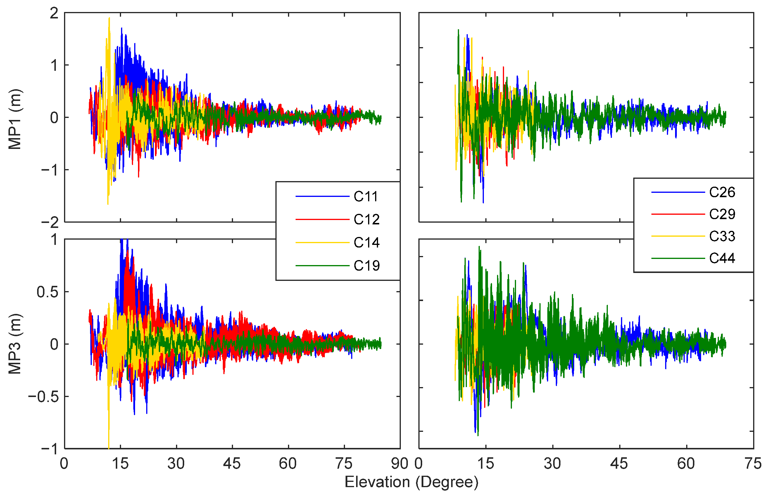
3.3. Reconstruction and Analysis of MP Deviations with Corrected Code Measurements

To verify the effectiveness of the previously established SCB correction model, the MP deviations were recalculated as a function of elevation angles on B1 and B3 frequencies for BDS IGSO satellites using corrected code observations (refer to Figure 7). The subfigure on the left displays the MP series of BDS-2 IGSO satellites (PRN: C06, C07, C09, and C10) launched before 2012, while the subfigure on the right shows the MP deviations of BDS-2/BDS-3 IGSO satellites (PRN: C13, C16, C39, and C40) launched after 2016. Due to the code multipath of surroundings and noise, there is a stochastic fluctuation, rather than a systematic bias, existing in the MP time series for all IGSO satellites on each frequency, especially in the conditions of low elevation. The maximum of MP1 deviations at these epochs can reach 1.0 m, while that of the MP3 series is no more than 0.5 m. Compared to the results from Figure 3, the MP deviations on B1 and B3 frequencies approach zero with increasing elevation, thereby indicating that the corrections of SCB on raw code observables for BDS IGSO satellites are valid and effective. Moreover, the MP series from BDS-2 to BDS-3 IGSO satellites exhibit similar characteristics, as there are no apparent differences between them after subtracting the SCB effect.

Figure 8 displays the MP deviations of BDS MEO satellites using corrected code measurements. The MP series of three BDS-2 MEO satellites (PRN: C11, C12, and C14, launched in 2012) and five BDS-3 MEO satellites (PRN: C19, C26, C29, C33, and C44, launched after 2017) are presented. The RMS of MP combinations on the B1 frequency is significantly larger than that on the B3 frequency, which may be attributed to the B3 frequency’s code rate being five times higher than that of the B1 frequency, despite both using QPSK modulation. Furthermore, even with improved code observables, the maximums of MP1 and MP3 from BDS-2 MEO satellites can reach 2.0 and 1.0 m, respectively, which is much larger than those from BDS-3 MEO satellites. Although there is no systematic bias observed in both MP1 and MP3 series, MP deviations of MEO satellites show significant fluctuations, particularly for BDS-2 MEO satellites, when compared to the results of IGSO satellites.

To further analyze the availability of the corrected code measurements, we list the RMS errors of the MP time series for BDS satellites using raw and corrected code observables in

Table 1. RMS errors of MP time series on B1 and B3 frequencies for BDS available satellites with and without SCB corrections.

BDS-2 PRN	Orbit Type	Launch Date	RMS of Raw Code		RMS of Corrected Code		Improvement
			B1	B3	B1	B3	B1	B3
C06	IGSO	1 August 2010	0.21	0.11	0.14	0.07	33.3%	36.4%
C07	IGSO	18 December 2010	0.16	0.09	0.14	0.06	12.5%	33.3%
C09	IGSO	27 July 2011	0.19	0.12	0.17	0.07	10.5%	41.7%
C10	IGSO	2 December 2011	0.22	0.09	0.16	0.06	27.3%	33.3%
C13	IGSO	30 March 2016	0.21	0.18	0.14	0.06	33.3%	66.7%
C16	IGSO	10 July 2018	0.21	0.13	0.15	0.07	28.6%	46.2%
C39	IGSO	25 June 2019	0.21	0.07	0.19	0.05	9.5%	28.6%
C40	IGSO	5 November 2019	0.13	0.06	0.13	0.06	0	0
C11	MEO	30 April 2012	0.54	0.30	0.16	0.21	70.4%	30.0%
C12	MEO	30 April 2012	0.45	0.25	0.27	0.17	40.0%	32.0%
C14	MEO	19 September 2012	0.35	0.18	0.26	0.14	25.7%	22.2%
C19	MEO	5 November 2017	0.19	0.06	0.19	0.05	0	16.7%
C26	MEO	29 July 2018	0.22	0.11	0.16	0.08	27.3%	27.3%
C29	MEO	30 March 2018	0.29	0.12	0.27	0.11	6.9%	8.3%
C33	MEO	19 September 2018	0.30	0.12	0.26	0.09	13.3%	25.0%
C44	MEO	23 November 2019	0.19	0.13	0.19	0.12	0	7.7%

. For BDS-2 IGSO satellites, the RMS errors of MP1 deviations using raw code measurements range from 0.16 to 0.22 m, whereas those of MP3 series using raw code measurements are much better (ranging from 0.09 to 0.18 m). For BDS-2 MEO satellites, the RMS errors of MP1 deviations range from 0.35 m to 0.54 m, while the RMS errors of MP3 deviations range from 0.18 m to 0.30 m.

After applying the SCB correction model, for BDS-2 IGSO satellites, the maximum improvement in RMS errors of MP1 and MP3 are 33.3% and 66.7%, respectively. For BDS-2 MEO satellites, with the corrected code measurements, the RMS errors of MP1 can be reduced by 70.4%, 40.0%, and 25.7% to 0.21, 0.17, and 0.14 m, respectively, which means that the code observations of BDS-2 MEO satellites are more susceptible to SCB. Compared with MP1, the improvement rates of MP3 only range from 22.2% (PRN: C14) to 32.0% (PRN: C12).

Compared with BDS-2 satellites, a reduction of below 28.6% in the RMS errors of MP deviations on BDS-3 satellites can be noticed, especially for BDS-3 MEO satellites, which reveals that the code observables from BDS-3 satellites are more resistant to the effect of SCB on both B1 and B3 frequencies.

3.4. Statistic and Analysis of Code Measurements with Epoch-Difference Method

Now that the systematic bias in the raw code observations has been corrected through the application of SCB, our attention turns to reducing the measurement noise present in the data. As the ED method has been widely used to remove the effects of stable biases for GNSS signals, the noise level of ED code can validate the effectiveness of the proposed smoothed method, and the formula can be expressed as follows [35]:

$$\{\begin{array}{c}\Delta {\epsilon }_{p_1}=\Delta P_1-\Delta {\varphi }_1-2\Delta I_1\\ \Delta {\epsilon }_{p_j}=\Delta P_j-\Delta {\varphi }_j-2\frac{f_1^2}{f_j^2}\Delta I_1\end{array}$$

(34)

with

$$\Delta I_1=\frac{\Delta {\varphi }_1-\Delta {\varphi }_j}{f_1^2/f_j^2-1}$$

(35)

where the subscript denotes the frequency ($j=2,3,\cdots$), $\Delta P$ is the ED code measurement, and $\Delta \varphi$ represents the time-differenced phase observable in meters.

With 24 h GNSS measurements from the Xia1 station (doy: 066), where the GNSS antenna remains stationary, the RMS errors of raw code, DSC, and RDSC on B1 (upper) and B3 (bottom) frequencies are provided in Figure 9 with the empirical assumptions (e.g., ${\sigma }_p$ = 0.3 m and ${\sigma }_D$ = 0.1 Hz). To show the RMS errors clearly, the intervals of the Y-axis are different. More specifically, the subfigures illustrate the noise level of code observations from BDS-2 IGSO satellites (PRN: C06-C10, C13, and C16) and MEO satellites (PRN: C11, C12, C14, and C24), respectively.

It is clear that the RMS errors of ED code measurements become larger with interval sampling increasing regardless of orbit types, especially when the sampling interval exceeds 5 s. With respect to the noise magnitude of the ED raw code, they are basically at the centimeter level, and the maximum of that is 16.5, 51.2, 94.4, 126.7, and 173.8 mm on B1 frequency, respectively, when the sampling intervals vary from 1 to 30 s. In comparison, the noise level on B3 frequency is better, and the maximum of the RMS errors is 11.1, 22.0, 37.4, 52.8, and 86.2 mm, respectively. After the introduction of Doppler observables, the maximum RMS error of ED-DSC on B1 frequency is 15.1, 47.9, 83.5, 110.3, and 158.8 mm, respectively. By contrast, the maximum RMS error of ED-DSC on B3 frequency is smaller than those on B1 frequency, which can be reduced −3.8, −26.8, −48.6 and −63.8 and −95.8 mm with intervals ranging from 1 to 30 s, respectively. These statistics reveal that the accuracy of ED-DSC is better than that of ED raw code, which can be explained well by the adoption of Doppler measurements. However, it should be noted that as the interval increases, this improvement becomes smaller or even worse, indicating that the integral cumulative error of the Doppler would affect the raw code accuracy with a large sampling interval.

For suppression of the gradually increased Doppler noise, a balance factor is adopted to refine the DSC, and the RMS errors of ED-RDSC are also represented in Figure 9. Compared with the results of DSC, the maximums of the RMS errors on B1 frequency are reduced by 4.8%, 1.2%, 1.8%, 8.3%, and 21.9% to 14.4, 47.3, 82.0, 101.1 and 124.0 mm, respectively. Meanwhile, the maximums of the RMS errors on B3 frequency are reduced by 3.9%, −0.3%, −0.5%, 1.0%, and 3.5%, respectively. Obviously, when the sampling interval is below 10 s, the integral cumulative error of the Doppler is not large enough to affect the code precision, leading to slight differences in RMS errors between DSC and RDSC. However, as the sampling interval gradually increases, the progressively amplified Doppler noise increases rapidly, causing a negative impact on the accuracy of the Doppler-aided smoothing code.

In addition, to verify the effectiveness of the Doppler-aided smoothing method in a high-dynamic scenario, one unmanned aerial vehicle (UAV) was used to obtain the real observables of BDS satellites. The UAV model used was Feima D20, equipped with the UM482 GNSS module produced by Unicore Communications. The GNSS module can only track B1 and B2 signals (2I/7I). The flying zone is located in Yulin City, Shaanxi Province, China. The UAV flew at an altitude of 400 m relative to the highest elevation point in the survey area, with a flying speed of approximately 16 m/s. The flying date was 1 June 2023 (doy: 151). The left subfigure in Figure 10 presents the overall appearance of the D20 drone, while the right one illustrates the corresponding flying track, excluding the takeoff and landing phases of the flight.

As pointed out by Zhou and Li (2017), constructing a reliable dynamic model for kinematic applications can present significant challenges. Therefore, the effectiveness of the proposed method is validated by assessing the accuracy of the ED code itself instead of analyzing SPP solutions that may heavily rely on dynamic models. Figure 11 showcases the RMS errors of ED code measurements for B1 (top) and B2 (bottom) signals from available BDS satellites during the UAV flight. The duration of the flight is just 40 min due to battery capacity constraints, excluding the time taken for takeoff and landing of the UAV. With a sampling interval of 0.05 s, there are theoretically 48,000 epochs. However, as the interval increases to 5 s, the number of epochs decreases to just one percent.

In order to conduct a thorough analysis of the smoothing effect, a total of five BDS satellites were carefully selected for continuous signal tracking. Among these, the raw B1 code exhibits the poorest performance, with RMS errors ranging from 45.2 to 218.7 mm as the interval varies from 0.05 to 5 s. Comparatively, the RMS errors of DSC show better performance than the raw code, particularly when the interval is below 5 s. However, as the Doppler noise gradually increases, the RMS error of DSC reaches 223.9 mm when the interval is set to 5 s. Nevertheless, the integration of a balance factor successfully reduces the RMS error of the RDSC by 5.8% to 210.9 mm. It is important to note that in the given scenario, the RMS errors of raw code measurements are better than those of Doppler-aided code. This suggests that the use of DSC or RDSC may not be suitable due to the larger sampling interval. A similar phenomenon can also be observed regarding the results of the B2 signals, with the only difference being that the RMS errors of C13 show poor performance regardless of the intervals.

It is indeed worth noting that in dynamic situations, the RMS errors of ED code measurements tend to be larger compared to static scenarios due to the increased complexity and challenges in tracking and processing signals. Factors such as satellite dynamics, receiver dynamics, multipath effects, and atmospheric conditions contribute to this increase in errors. However, despite the higher noise level in measurements, based on the aforementioned findings, we can conclude that Doppler measurements have the potential to enhance the accuracy of raw code observations, even with significant limitations in the smooth window. By taking into account the balance factor, the progressively amplified Doppler noise can be suppressed, enabling the successful utilization of RDSC in challenging environments. Additionally, limiting the sampling interval is recommended (e.g., to exceed 20 Hz) in order to ensure the effectiveness of Doppler-aided smoothing code methods, particularly in high-dynamic scenarios.

It is noticed that the SCB correction model is not considered in this section. The main reason is that the SCB model is elevation-dependent and established by a polynomial segment fitting algorithm (see Equation (21)), which means that the SCB corrections between consecutive epochs are basically identical because of the similar elevation angles, and then the SCB corrections would be removed with the ED method.

3.5. Positioning Accuracy of SPP with BDS-2 Code Measurements

In this section, the positioning performance of stand-alone positioning is provided with real measurements from the XIA1 station. In consideration of the weighted least square method, four schemes have been designed to calculate SPP: (1) raw code; (2) CSC; (3) DSC; and (4) RDSC. For a fair comparison, the smoothing window of the above schemes is set at two, and Klobuchar and Saastamoninen models are applied to weaken the atmospheric delays. It should be noted that one GEO satellite (PRN: C05) is excluded because of its unhealthy status, and one IGSO satellite (PRN: C06) is also excluded due to its frequent data loss.

The available satellite numbers (PRN: C01-C04, C07-C14, and C16) and the horizontal and vertical dilutions of precision (HDOP and VDOP) are shown in Figure 12. We noticed that the change in the available satellites results in a variation in the dilution of precision (DOP). For illustrative purposes, the final standard point positioning solution with dual-frequency phase observations is used as a reference, and then the RMS errors for three directions calculated by Equation (36) with changing sampling intervals for the above schemes are presented in Figure 11. The 3D RMS errors can be computed by

$$RMS\left(3D\right)=\sqrt{RMS{\left(E\right)}^2+RMS{\left(N\right)}^2+RMS{\left(U\right)}^2}$$

(36)

The scheme (1) with raw code in Figure 13 usually produces the worst positioning results, and the RMS errors in the east, north, and up directions can reach 1.51, 2.28, and 4.20 m, respectively, which remain almost the same despite the changing sampling intervals. On the contrary, during the increase in sampling intervals, the RMS errors of the scheme (2) with CSC progressively decrease, and they are better than 1.11, 2.26, and 4.07 m, respectively, which can be explained well by the reduction in thermal noise. Similarly, the RMS errors of scheme (3) with DSC become smaller with an increasing sampling interval, especially in situations with small intervals. However, as a result of the integral cumulative error of the Doppler observable, the RMS errors of DSC significantly increase when the sampling interval exceeds 45 s, especially in the north and up directions. When the interval is 90 s, the 3D RMS error of DSC is 5.09 m, which is raised by 3.7% in comparison with that of the raw code. Due to the introduction of the balance factor, the RMS errors of RDSC are better than those of DSC when the sampling interval is more than 15 s, indicating that the balance factor can effectively adjust the contribution of raw code and smoothed code measurements.

For comparative analysis, the SPP performance of SCB with and without SCB correction is listed in

Table 2. RMS statistics of positioning errors in east, north, and up directions for BDS-2 satellites using RDSC with and without SCB correction (unit: m).

Interval (Second)	RMS of RDSC			RMS of RDSC-SCB			3D Improvement Rate (%)
	East	North	Up	East	North	Up
1	1.153	2.269	4.162	1.111	2.312	3.693	0.68/8.46
15	1.133	2.256	4.122	1.186	2.299	3.716	1.57/6.20
30	1.139	2.262	4.159	1.195	2.286	3.752	0.81/5.44
45	1.144	2.266	4.172	1.200	2.289	3.773	0.60/5.13
60	1.144	2.267	4.173	1.203	2.291	3.772	0.45/5.19
75	1.147	2.270	4.186	1.207	2.309	3.781	0.37/5.00
90	1.148	2.268	4.185	1.206	2.303	3.815	0.35/4.58

. The RMS errors of RDSC without SCB correction in the east, north, and up directions are given in columns 2 to 4, while the ones of RDSC with SCB correction (RDSC-SCB) are given in columns 5 to 7. Compared with the positioning statistics of raw code measurements, the improvement rates of RDSC and RDSC-SCB are presented in the last column. Regarding the SPP positioning precision, they are at the meter level for RDSC, the mean RMS errors of which are 1.14, 2.26, and 4.17 m, respectively. Owing to the adjustment of the balance factor, the differences in RMS errors between raw code and RDSC are getting smaller, and the improvement rates are closer to zero with sampling intervals increasing from 1 to 90 s. After the application of SCB correction, the mean RMS errors in the east and north directions increased by 3.75% and 1.46% to 1.187 and 2.298 m, respectively, whereas the mean RMS error in the up direction was reduced by 10.14% to 3.743 m. The main reason may be that the effect of SCB on up direction is larger than that on horizontal directions in the user end, which coincides with the characteristics of the multipath effect by previous research.

4. Discussion

The noise level of raw code observables from BDS satellites is limited by thermal noise and systematic bias. To mitigate the former, the CSC filter has gained widespread usage in GNSS preprocessing processors, assuming that carrier measurements lack cycle slips. However, meeting this assumption becomes challenging in adverse environments. The robustness and immunity of the Doppler measurement to cycle slips make it suitable for smoothing raw code observations resembling CSC. However, as the sampling interval increases, the precision of DSC decreases due to gradually increased Doppler noise. To address this issue, a balance factor is introduced to adjust the contributions of raw code and DSC based on the principle of minimal variance. This adjustment enhances the reliability of SPP, particularly in the up direction. Therefore, in challenging GNSS scenarios, including both static and dynamic cases, the utilization of Doppler-aided smoothing code may hold more promise for enhancing navigation and positioning applications.

The code measurements of BDS satellites suffer from systematic bias (SCB), which has proved to be dependent on elevation angles and carrier frequency. Therefore, in this paper, by minimizing the sum of the absolute value of residuals, a polynomial segment fitting algorithm is adopted to establish SCB correction as a function of elevation angles for available BDS-2 and BDS-3 un-GEO satellites and each frequency. After applying the SCB correction model, the RMS values of the MP series can be significantly reduced. For BDS-2 IGSO satellites, compared with MP1 deviations using raw code, the improvement rate of RMS errors of MP1 deviations can reach up to 66.7%. For BDS-2 MEO satellites, a reduction of 70.4% in the RMS errors of MP1 can be obtained. In addition, by contrast with MP1, the RMS errors of MP3 are obviously smaller than those of MP1, and most of the improvement rates are no more than 32.0%. In the code measurements of BDS-3 satellites, it is still possible to observe strong elevation-dependent SCB variances. However, the level of SCB is just around 0.1m, resulting in insignificant improvement rates except for a 27.3% improvement on both legacy signals for C19. These numerical experiments indicate that code measurements of MEO satellites are more vulnerable to SCB compared to IGSO satellites. Additionally, the code observables on the B3 frequency exhibit greater resistance to SCB compared to the B1 frequency.

The positioning accuracies of the raw code are 1.514, 2.275, and 4.202 m, respectively, while the RMS errors of the CSC are better than 1.111, 2.259, and 4.071 m, respectively. Similarly, SPP with DSC performs well in situations with smaller intervals. However, when the interval increases from 45 to 90 s, the 3D RMS error of DSC becomes the worst (5.094 m). Due to the introduction of the balance factor, the RMS errors of RDSC outperform those of DSC when the sampling interval is more than 15 s. After the application of SCB correction, the mean RMS errors in the east and north directions increased by 3.75% and 1.46% to 1.187 and 2.298 m, respectively, whereas the mean RMS error in the up direction was reduced by 10.14% to 3.743 m. One possible reason is that the SCB correction models are simply established for BDS un-GEO satellites except for GEO satellites, leading to a decrease in the SPP precision.

Due to the unique orbit characteristics of GEO satellites, there has been relatively less focus on developing SCB correction models specifically for these satellites, which will be the focus of our future research. Then, with continuous improvement in the SCB model for each BDS satellite, better navigation and stand-alone positioning performance with code observations would be more promising.

5. Conclusions

As the Doppler measurement is robust and immune to cycle slip, it can be used to smooth raw code observation that resembles CSC. Compared with raw code and CSC, the noise level and positioning accuracy of DSC can be improved, especially in the situation of high sampling frequency. However, when the sampling interval increases, the precision of DSC decreases due to the relatively large Doppler noise. Therefore, a balance factor is introduced to adjust the contributions of raw code and DSC, which can be helpful in enhancing the reliability of SPP. When GNSS receivers are utilized in challenging scenarios, such as in urban environments or under heavy foliage, the integration of Doppler-aided smoothing code techniques has the potential to provide more reliable and accurate navigation and positioning services.

The smoothed filter, such as the CSC and DSC, can significantly enhance the precision of code measurements by assuming that the measurement noise follows a zero-mean Gaussian distribution. However, this assumption can be violated by the SCB effect present in the code measurements of BDS satellites. As a result, extensive research was conducted to investigate the SCB variations of un-GEO satellites, and applying the SCB correction model for each un-GEO satellite and frequency was found to effectively reduce the RMS values of MP series and improve SPP performance.

Despite these efforts, few studies have focused on developing an SCB correction model for GEO satellites, owing to their unique orbit characteristics. Therefore, our future research will aim to address this issue and develop an effective SCB correction model for GEO satellites. With continuous improvements in the SCB model for each BDS satellite, we can expect a significant enhancement in the performance of navigation and stand-alone positioning with code observations.

References

1. Hofmann-Wellenhof, B.; Lichtenegger, H.; Collins, J. Global Positioning System: Theory and Practice, 5th ed.; Springer: New York, NY, USA, 2001; pp. 181–188. [Google Scholar]
2. Xu, G.; Xu, Y. Parameterization and algorithms of GPS data processing. In GPS Theory, Algorithms and Applications, 3rd ed.; Springer: New York, NY, USA, 2016; pp. 291–300. [Google Scholar]
3. Won, J.H.; Pany, T. Signal processing. In Springer Handbook of Global Navigation Satellite Systems, 1st ed.; Teunissen, P.J.G., Montenbruck, O., Eds.; Springer: New York, NY, USA, 2017; pp. 428–434. [Google Scholar]
4. Hatch, R. The synergism of GPS code and carrier measurements. In Proceedings of the 3rd International Geodetic Symposium on Satellite Doppler Positioning, Las Cruces, NM, USA, 8–12 February 1982. [Google Scholar]
5. Hatch, R. Dynamic differential GPS at the centimeter level. In Proceedings of the 4th International Geodetic Symposium on Satellite Positioning, Austin, TX, USA, 28 April–2 May 1986. [Google Scholar]
6. Hwang, P.Y.; McGraw, G.A.; Bader, J.R. Enhanced differential GPS carrier-smoothed code processing using dual-frequency measurements. Navigation 1999, 46, 127–138. [Google Scholar] [CrossRef]
7. Bisnath, S.B.; Langley, R.B. High-precision, kinematic positioning with a single GPS receiver. Navigation 2002, 49, 161–169. [Google Scholar] [CrossRef]
8. Park, B.; Sohn, K.; Kee, C. Optimal Hatch filter with an adaptive smoothing window width. J. Navig. 2008, 61, 435–454. [Google Scholar] [CrossRef]
9. Gunther, C.; Henkel, P. Reduced-noise ionosphere-free carrier smoothed code. IEEE Trans. Aerosp. Electron. Syst. 2010, 46, 323–334. [Google Scholar] [CrossRef]
10. Gao, X.; Yang, Z.; Du, Y.; Yang, B. An improved real-time cycle slip correction algorithm based on Doppler-aided signals for BDS triple-frequency measurements. Adv. Space Res. 2021, 67, 223–233. [Google Scholar] [CrossRef]
11. Geng, J.; Jiang, E.; Li, G.; Xin, S.; Wei, N. An Improved Hatch Filter Algorithm towards SubMeter Positioning Using only Android Raw GNSS Measurements without External Augmentation Corrections. Remote Sens. 2019, 11, 1679. [Google Scholar] [CrossRef] [Green Version]
12. Cheng, P. Remarks on Doppler-aided smoothing of code ranges. J. Geod. 1999, 73, 23–28. [Google Scholar] [CrossRef]
13. Kubo, N. Advantage of velocity measurements on instantaneous RTK positioning. GPS Solut. 2009, 13, 271–280. [Google Scholar] [CrossRef] [Green Version]
14. Chen, C.; Chang, G.; Luo, F.; Zhang, S. Dual-frequency carrier smoothed code filtering with dynamical ionospheric delay modeling. Adv. Space Res. 2019, 63, 857–870. [Google Scholar] [CrossRef]
15. Bruton, A.M.; Glennie, C.L.; Schwarz, K.P. Differentiation for high-precision GPS velocity and. acceleration determination. GPS Solut. 1999, 2, 7–21. [Google Scholar] [CrossRef]
16. Lee, H.; Rizos, C.; Jee, G.I. Position domain filtering and range domain filtering for carrier-smoothed-code DGNSS: An analytical comparison. IEE Proc. Radar Sonar Navig. 2005, 152, 271–276. [Google Scholar] [CrossRef] [Green Version]
17. Zhang, J.; Zhang, K.; Grenfell, R.; Deakin, R. Short note: On the relativistic Doppler effect for precise velocity determination using GPS. J. Geod. 2006, 80, 104–110. [Google Scholar] [CrossRef]
18. Zhang, X.; Guo, B.; Guo, F.; Du, C. Influence of clock jump on the velocity and acceleration estimation with a single GPS receiver based on carrier-phase-derived Doppler. GPS Solut. 2013, 17, 549–559. [Google Scholar] [CrossRef]
19. Bahrami, M.; Ziebart, M. A Kalman filter-based Doppler-smoothing of code pseudoranges in GNSS-challenged environments. In Proceedings of the 24th International Technical Meeting of the Satellite Division of the Institute of Navigation (ION GNSS 2011), Portland, OR, USA, 19–23 September 2011. [Google Scholar]
20. Zhou, Z.; Li, B. Optimal Doppler-aided smoothing strategy for GNSS navigation. GPS Solut. 2017, 21, 197–210. [Google Scholar] [CrossRef]
21. Zhang, K.; Jiao, W.; Wang, L.; Li, Z.; Li, J.; Zhou, K. Smart-RTK: Multi-GNSS kinematic positioning approach on android smart devices with Doppler-smoothed-code filter and constant acceleration model. Adv. Space Res. 2019, 64, 1662–1674. [Google Scholar] [CrossRef]
22. Zhou, H.; Li, Z.; Liu, C.; Xu, J.; Li, S.; Zhou, K. Assessment of the performance of carrier-phase and Doppler smoothing code for low-cost GNSS receiver positioning. Results Phys. 2020, 19, 103574. [Google Scholar] [CrossRef]
23. Li, R.; Zheng, S.; Wang, E.; Chen, J.; Feng, S.; Wang, D.; Dai, L. Advances in BeiDou Navigation Satellite System (BDS) and satellite navigation augmentation technologies. Satell. Navig. 2020, 1, 12. [Google Scholar] [CrossRef]
24. Yang, Y.; Ren, X.; Jia, X.; Sun, B. Development trends of the national secure PNT system based on BDS. Sci. China Earth Sci. 2023, 66, 929–938. [Google Scholar] [CrossRef]
25. Hauschild, A.; Montenbruck, O.; Sleewaegen, J.M.; Huisman, L.; Teunissen, P.J.G. Characterization of COMPASS M-1 signals. GPS Solut. 2012, 16, 117–126. [Google Scholar] [CrossRef]
26. Wanninger, L.; Beer, S. BeiDou satellite-induced code pseudorange variations: Diagnosis and therapy. GPS Solut. 2015, 19, 639–648. [Google Scholar] [CrossRef] [Green Version]
27. Lei, W.; Wu, G.; Tao, X.; Bian, L.; Wang, L. BDS satellite-induced code multipath: Mitigation and assessment in new-generation IOV satellites. Adv. Space Res. 2017, 60, 2672–2679. [Google Scholar] [CrossRef]
28. Guo, F.; Li, X.; Liu, W. Mitigating BeiDou Satellite-Induced Code Bias: Taking into Account the Stochastic Model of Corrections. Sensors 2016, 16, 909. [Google Scholar] [CrossRef] [Green Version]
29. Lou, Y.; Gong, X.; Gu, S.; Zheng, F.; Feng, Y. Assessment of code bias variations of BDS triple-frequency signals and their impacts on ambiguity resolution for long baselines. GPS Solut. 2017, 21, 177–186. [Google Scholar] [CrossRef]
30. Zou, X.; Li, Z.; Li, M.; Tang, W.; Deng, C.; Chen, L.; Wang, C.; Shi, C. Modeling BDS pseudorange variations and models assessment. GPS Solut. 2017, 21, 1661–1668. [Google Scholar] [CrossRef]
31. Pan, L.; Guo, F.; Ma, F. An improved bds satellite-induced code bias correction model considering the consistency of multipath combinations. Remote Sens. 2018, 10, 1189. [Google Scholar] [CrossRef] [Green Version]
32. Zhang, X.; Li, X.; Lu, C.; Wu, M.; Pan, L. A comprehensive analysis of satellite-induced code bias for BDS-3 satellites and signals. Adv. Space Res. 2019, 639, 2822–2835. [Google Scholar] [CrossRef]
33. McGraw, G.A. Generalized divergence-free carrier smoothing with applications to dual frequency differential GPS. Navigation 2009, 56, 115–122. [Google Scholar] [CrossRef]
34. Shu, B.; Liu, H.; Xu, L.; Gong, X.; Qian, C.; Zhang, M.; Zhang, R. Analysis of satellite-induced factors affecting the accuracy of the BDS satellite differential code bias. GPS Solut. 2017, 21, 905–916. [Google Scholar] [CrossRef]
35. Zhou, R.; Hu, Z.; Zhao, Q.; Li, P.; Wang, W.; He, C.; Cai, C.; Pan, Z. Elevation-dependent pseudorange variation characteristics analysis for the new-generation BeiDou satellite navigation system. GPS Solut. 2018, 22, 60. [Google Scholar] [CrossRef]
Figure 1. Traditional Hatch filter algorithm diagram.
Remotesensing 15 03549 g001
Figure 2. Relationship between sampling interval and SW ( σ p = 0.3 m and σ D = 0.1 Hz).
Remotesensing 15 03549 g002
Figure 3. Relationship between the sampling interval and balance factor (Upper: σ p = 0.3 m and σ D = 0.1 Hz; Bottom: σ p = 1.0 m and σ D = 0.1 Hz).
Remotesensing 15 03549 g003
Figure 4. Flowchart of the refined model for Doppler-aided smoothed code.
Remotesensing 15 03549 g004
Figure 5. MP time series (blue) and elevation angles (red) of BDS-2 IGSO satellites as a function of time using raw code measurements (left: C07; right: C16).
Remotesensing 15 03549 g005
Figure 6. MP time series and elevation angles of BDS MEO satellites as a function of time using raw code measurements (left: C12; right: C24).
Remotesensing 15 03549 g006
Figure 7. MP time series of BDS IGSO satellites as a function of elevation angles using improved code measurements corrected by previously established SCB correction model (upper: MP1; bottom: MP3).
Remotesensing 15 03549 g007
Figure 8. MP time series of BDS MEO satellites as a function of elevation angles using improved code measurements corrected by previously established SCB correction model (upper: MP1; bottom: MP3).
Remotesensing 15 03549 g008
Figure 9. RMS errors of ED code measurements for BDS satellites in a static scenario (left: raw code; middle: DSC; and right: RDSC).
Remotesensing 15 03549 g009
Figure 10. UAV model and its corresponding flying track on 1 June 2023.
Remotesensing 15 03549 g010
Figure 11. RMS errors of ED-code measurements for BDS satellites in a high-dynamic scenario (Left: raw code; Middle: DSC; Right: RDSC).
Remotesensing 15 03549 g011
Figure 12. Number of available satellites, HDOP, and VDOP series using dataset collected at XIA1 station on 7 March 2023 (sampling interval: 1 s).
Remotesensing 15 03549 g012
Figure 13. RMS errors of SPP in east, north, and up directions with different sampling intervals using BDS raw code and smoothed code measurements.
Remotesensing 15 03549 g013