Article

Optical and SAR Image Registration Based on Pseudo-SAR Image Generation Strategy

1
College of Information Science and Technology, Beijing University of Chemical Technology, Beijing 100029, China
2
Beijing Advanced Innovation Center for Soft Matter Science and Engineering, Beijing University of Chemical Technology, Beijing 100029, China
*
Author to whom correspondence should be addressed.
Remote Sens. 2023, 15(14), 3528; https://doi.org/10.3390/rs15143528
Submission received: 1 June 2023 / Revised: 28 June 2023 / Accepted: 11 July 2023 / Published: 13 July 2023
(This article belongs to the Special Issue SAR Images Processing and Analysis)

Abstract

:
The registration of optical and SAR images has always been a challenging task due to the different imaging mechanisms of the corresponding sensors. To mitigate this difference, this paper proposes a registration algorithm based on a pseudo-SAR image generation strategy and an improved deep learning-based network. The method consists of two stages: a pseudo-SAR image generation strategy and an image registration network. In the pseudo-SAR image generation section, an improved Restormer network is used to convert optical images into pseudo-SAR images. An L2 loss function is adopted in the network, and the loss function fluctuates less at the optimal point, making it easier for the model to reach the fitting state. In the registration part, the ROEWA operator is used to construct the Harris scale space for pseudo-SAR and real SAR images, respectively, and each extreme point in the scale space is extracted and added to the keypoint set. The image patches around the keypoints are selected and fed into the network to obtain the feature descriptor. The pseudo-SAR and real SAR images are matched according to the descriptors, and outliers are removed by the RANSAC algorithm to obtain the final registration result. The proposed method is tested on a public dataset. The experimental analysis shows that the average value of NCM surpasses similar methods over 30%, and the average value of RMSE is lower than similar methods by more than 0.04. The results demonstrate that the proposed strategy is more robust than other state-of-the-art methods.

Graphical Abstract

1. Introduction

Optical and synthetic aperture radar (SAR) images are two types of products formed by distinct sensors. Optical images result from the passive reception of naturally reflected light, while SAR images are generated by actively transmitting and receiving radar electromagnetic waves. The quality of optical images is heavily affected by cloudy conditions and night variations. In contrast, SAR is capable of observing the earth under various weather conditions and demonstrates strong performance during day and night. Therefore, it is necessary to jointly use the effective information from these two different imaging sensors. Thus, how to match the two kinds of images becomes the top priority. However, SAR images often exhibit unique manifestations, such as shadows, superimposition, and foreshortening, which are caused by special imaging mechanisms. These imaging disparities pose challenges to the registration of optical and SAR images.
In recent years, many researchers have proposed diverse approaches for matching optical and SAR images [1]. Presently, three primary frameworks for the image registration have been established [2]: area-based matching [3], feature-based matching [4], and deep learning-based matching methods [5].
Area-based matching techniques rely on template matching to quantify the similarity of image block templates, employing similarity metrics such as mutual information [6,7,8], normalized cross-correlation coefficient [9,10], and cross-cumulative residual entropy [11].
Although area-based matching methods tend to achieve higher accuracy than feature-based methods in homologous image registration due to their use of the gray-scale information of image regions, they are sensitive to the nonlinear radiometric differences between optical and SAR images. Additionally, the need to traverse the entire reference image in area-based registration methods results in computationally complexity. Consequently, there are some limitations to the registration of optical and SAR images using area-based methods [12].
Feature-based matching is also an important method framework in image registration. This method is mainly divided into four steps: keypoint extraction, feature descriptor construction, feature matching, and affine transformation. Generally, feature-based matching methods have a higher calculation speed than area-based matching methods. The most famous one is the scale-invariant feature transform (SIFT) [13] method. It has good effects on rotation, scaling, translation, and shall be robust to intensity changes and affine distortion. The different imaging mechanisms of optical and SAR images, such as noise characteristics, may cause distortions in the keypoint detection and matching by just using SIFT. In the research on applying the SIFT algorithm to optical and SAR image registration, some scholars have made attempts. Xiang et al. proposed OS-SIFT [14,15,16], which improved the method of extracting keypoints from SAR images and built a new descriptor. Sedaghat et al. established an improved descriptor-based framework called UR-SIFT [17]. Ma et al. [18] adopted a new gradient calculation architecture, which introduced an enhanced feature-matching method based on the position, scale, and orientation of each keypoint. However, the traditional feature-matching strategy mentioned above is challenging to eliminate the offset of matched point pairs caused by feature differences.
With the development of artificial intelligence, deep learning technology has gradually been applied to the registration of remote sensing images from different sources. Compared with traditional methods, deep learning-based descriptor construction methods have stronger robustness and are more conducive to keypoint matching [2]. Han et al. [19] proposed a Siamese network, which uses image blocks to construct feature vector descriptors. It has been widely applied in the registration field. Subsequently, numerous deep learning-based registration methods emerged, such as TFeat [20], L2 Net [21], HardNet [22], MatchosNet [23], etc. Xiang et al. [24] proposed a new registration method based on feature and area combinations. The above deep learning-based methods have made significant progress in the feature-based registration field, but there are also some limitations. When dealing with significant feature differences between optical and SAR images, it will lead to an offset of matched point pairs.
To mitigate the feature differences, several scholars have proposed image transformation-based methods. For instance, Maggiolo et al. [25] employed a conditional GAN-based generation strategy to convert optical images into SAR images and then conducted a template matching between the GAN-generated SAR and real SAR images. Huang et al. [26] utilized a CycleGAN network structure to transform SAR images into pseudo-optical images and registered them with real optical images. Many researchers have also explored the potential of the Transformer model [27], which was introduced by Google in 2017, for SAR image processing. Self-attention mechanisms [28,29,30,31] included by the Transformer network, which are used to replace the conventional convolution operator, have been employed in SAR image [32,33,34] interpretation. The attention mechanism allows the network to extend information beyond the convolution kernel’s range in the surrounding space, resulting in a more robust feature extraction of spatial relations, particularly for high-resolution images [35]. It can further focus on the imaging differences between optical and SAR images, greatly increasing the success probability of transforming optical images into pseudo-SAR images [27]. In the Transformer architecture, self-attention mechanisms are used instead of CNN structures in the encoder and decoder. This paper employs a Transformer model for pseudo-SAR image generation; then, it seeks registration between pseudo-SAR and real SAR images.
To address the registration of homologous SAR images, in the field of traditional methods, Schwind et al. [36] combined the Best-Bin-First algorithm with SIFT for SAR image registration. Delinger et al. proposed the SAR-SIFT [37] method, which replaced the DoG pyramid with the Harris pyramid and utilized the ratio gradient [38,39], achieving good results in SAR image registration. These traditional methods based on SAR image gray-scale variations struggle to detect effective keypoints in SAR images with narrow dynamic ranges, but they could lead to unsatisfied results sometimes. In the field of deep learning, Du et al. [40] introduced FM-CycleGAN to achieve feature-matching consistency. Ye et al. [5] achieved remote sensing image registration by fusing SIFT and CNN feature descriptors. However, as the convolutional layers deepen, detail features in SAR images are gradually lost. Effectively utilizing these detail features has become a research direction in SAR image registration. Yun et al. [23] presented an improved Siamese [19] network, called MatchosNet, to avoid the loss of detail features. In proposed framework, a refined scheme including MatchosNet is constructed in the registration stage between pseudo-SAR and real SAR images.
Inspired from the Transformer and the MatchosNet, this paper presents a novel method for the registration of optical and SAR images, adopting a pseudo-SAR generation strategy and an improved registration network between pseudo-SAR and real SAR images. The overall methodology is illustrated in Figure 1. In the first step, an improved Restormer [41] network is utilized to transform optical images to pseudo-SAR images. This network originated from Transformer and comprises several encoding and decoding blocks, which are each equipped with self-attention mechanisms. These mechanisms effectively capture the feature differences present in the local features of optical and SAR images. To enhance performance, we adopt the L2 loss function, which facilitates better estimating similarity between the pseudo-SAR and real SAR images, aiding the convergence of network weights toward an optimal fitting state. In the second step, the registration is conducted between the pseudo-SAR and real SAR images. Initially, the ROEWA [16] operator is applied to construct a multi-scale Harris scale space for both images. Subsequently, extremal points are selected from each scale space and incorporated into the keypoint sets obtained from the pseudo-SAR and real SAR images. The ROEWA operator effectively extracts informative features from SAR images, while the Harris scale space construction facilitates the extraction of keypoints at multiple scales, thereby enhancing the robustness of the extracted keypoints. For each keypoint in the pseudo-SAR and real SAR image keypoint sets, an image patch surrounding it is extracted and fed into the MatchosNet network. The network employs deep feature extraction, resulting in the generation of robust descriptor vectors. MatchosNet utilizes a twin-branch network with shared weights, enabling the maximum utilization of feature information from both pseudo-SAR and real SAR images, thereby producing optimal descriptor matches. Finally, the RANSAC [42] algorithm is employed to eliminate outlier matching pairs. The contributions of this paper are as follows:
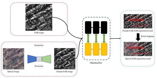
  • In the pseudo-SAR generation strategy, this paper use the improved Restormer network to eliminate the feature differences between optical and SAR images.
  • For the registration part, a refined keypoint extraction method using the ROEWA operator is designed to construct the Harris scale space and used to extract the extreme points in each scale.
The remaining sections of this paper are organized as follows. Section 2 provides a detailed description of the proposed method. The results of registration and the ablation experiment are presented in Section 3. Section 4 shows the experimental results and a discussion of research prospects. Conclusions are given in Section 5.

2. Materials and Methods

As Figure 1 shows, the schematic diagram of our proposed method consists of two main parts. Firstly, this paper adopts an improved Restormer to accomplish our pseudo-SAR generation strategy, transforming optical images into pseudo-SAR images. Secondly, the Harris scale space is constructed for both pseudo-SAR and real SAR images using the ROEWA operator, and we extract extremal points in each scale space. And then, image patches are selected around the keypoints, and we input them into the MatchosNet network to obtain robust descriptors. Based on the feature descriptors, keypoints are matched in pseudo-SAR and real SAR images, and we utilize the RANSAC algorithm to eliminate outliers, resulting in the final matching results.

2.1. Pseudo-SAR Image Generation Strategy

2.1.1. Network Architecture

Inspired by the Restormer network, a deep learning-based transformation method is proposed. Specifically, an encoder network is employed to extract feature information from the optical image and a decoder to decode the feature information. Within the encoder–decoder network, the transposed self-attention mechanism is used to enhance the model’s robustness of the feature differences in optical and SAR images. Finally, a pseudo-SAR image consistent with the feature imaging of real SAR images is obtained. The specific network structure is illustrated in Figure 2.
As shown in Figure 2, the input to the network is an optical image to be transformed, and the output is a pseudo-SAR image. The input image is first processed by convolution to expand the number of channels to obtain a high-dimensional feature matrix. These features are then transformed into deeper feature maps through a symmetric encoder–decoder at each level. There are a total of four levels of corresponding to the encoder and decoder blocks. Each level of encoder and decoder has multiple Transformer blocks. The number of Transformer blocks gradually increases from top to bottom, mainly for deep feature extraction. The attention mechanism establishes a connection between local and global features. The encoder uses downsampling to continuously reduce the spatial size of the input image and increase feature dimension. The decoder employs upsampling to progressively enlarge the image while compressing the feature dimensions. In order to transfer the features extracted from each downsampling layer, skip connections are added after each downsampling layer, and the feature matrix obtained by upsampling are concatenated in the channel dimension and compressed by convolution. Then, the feature matrix is further refined through several Transformer blocks and a convolution layer. To better learn the differences between the optical and SAR image features, the network introduces element-wise operation between the original optical image feature and the high-level feature matrix to help restore the lost texture and semantic details in the image. Finally, the network outputs the generated pseudo-SAR image.
The structure of the Transformer block is shown in Figure 3, which includes two modules, MDTA [41] and GDFN. The MDTA module is Multi-Dconv Head Transposed Attention. The main network structure of this module is a self-attention mechanism. Firstly, normalize the input feature matrix, and then generate Q, K, V projections through 1 × 1 point-wise convolution and 3 × 3 depth-wise convolution, respectively. Here, Q projection is query projection, K projection is keyword projection, and V is value projection. Then, multiply the Q and K matrices to obtain the Transposed Attention Map. The Transposed Attention Map is element-wise multiplied with the V, and the resulting matrix is obtained through 1 × 1 point-wise convolution to generate the output matrix of MDTA. The principle formula is as follows:
X ^ = W p   Attention   ( Q ^ , K ^ , V ^ ) + X Attention ( Q ^ , K ^ , V ^ ) = V ^ Softmax ( K ^ Q ^ )
where X and X ^ are the input and output vector feature maps, respectively, and the Q ^ R H ^ W ^ × C ^ , K ^ R C ^ × H ^ W ^ , and V ^ R H ^ W ^ × C ^ matrices are obtained by transformation from the original matrix R H ^ × W ^ × C ^ .
The GDFN module is Gated Dconv Feedforward Network [41]. As shown in Figure 3, the GDFN structure is divided into two parallel paths. Both paths undergo 1 × 1 convolution and 3 × 3 depth convolution. One of the paths is nonlinear activated by the GELU. Finally, the outputs of the two paths are multiplied element-wise and passed through a 1 × 1 convolution layer. The resulting matrix is then added element-wise to the input matrix to obtain the output matrix. The corresponding formula for this method is as follows:
X ^ = W p 0 Gating ( X ) + X Gating ( X ) = ϕ W d 1 W p 1 ( LN ( X ) ) W d 2 W p 2 ( LN ( X ) )
where represents the multiplication of each element in the vector, and ϕ represents the nonlinear GELU function. LN is a layer normalization operation. W p ( ) is 1 × 1 pixel by pixel convolution, and W d ( ) is 3 × 3 convolution.

2.1.2. Pseudo-SAR Generation Network Loss Function

In the application of Restormer to optical image, an L1 loss function is usually employed. Compared to the L1 loss function, the L2 loss function emphasizes the penalization of erroneous pixels, resulting in smoother fluctuations around the best fit in the model [43,44]. The later experiments will further demonstrate its effectiveness. Therefore, the L2 loss function is used here to calculate the difference between the pseudo-SAR and real SAR image. The formula for the L2 loss function is given below:
Loss ( x , y ) = 1 n m i = 1 n j = 1 m y i j f x i j 2
where y i j is the pixel values of real SAR images at coordinates ( i , j ) , and f x i j is the pixel values of pseudo-SAR image at coordinates ( i , j ) . n and m represent the size parameters of images.

2.1.3. Pseudo-SAR Generation Performance Evaluation

The performance evaluation of the pseudo-SAR generation strategy is conducted using a combination of subjective visual assessment and objective evaluation metrics. The objective quantitative evaluation indicators used for testing are the Average Gradient (AG), Structural Similarity (SSIM), Peak Signal-to-noise Ratio (PSNR), Learned Perceptual Image Patch Similarity (LPIPS) [45], and Mean Absolute Error (MAE) index. The pseudo-SAR image and results of these indicators will also be mentioned in the ablation experiments.
(1)
AG
The Average Gradient index is calculated using the following formula:
A G = 1 m × n i = 1 m j = 1 n Δ I x 2 + Δ I y 2 2
where m and n are the size parameters of the image, and Δ I x and Δ I y are the differences on the horizontal and vertical coordinates, respectively. The AG reflects the difference in gray-scale near the edge of an image and is used to measure the clarity of the image, and a larger value represents a clearer image.
(2)
SSIM
The formula for SSIM is given as follows:
S S I M ( x , y ) = 2 μ x μ y + c 1 2 σ x y + c 2 μ x 2 + μ y 2 + c 1 σ x 2 + σ y 2 + c 2 c 1 = k 1 L 2 c 2 = k 2 L 2
where μ x is the mean of x , μ y is the mean of y , σ x 2 is the variance of x , σ y 2 is the variance of y , σ x y is the covariance of x and y , and c 1 and c 2 are used to maintain stability in the dynamic range of pixel values. Among c 1 and c 2 , L is the dynamic value range of the pixel value, k 1 and k 2 represent the hyperparameters, which are generally 0.01 and 0.03. In this evaluation indicator, a value closer to 1 indicates a higher similarity between the pseudo-SAR and the real SAR image.
(3)
PSNR
Regarding PSNR, the formula is given as follows:
M S E = 1 m n i = 0 m 1 j = 0 n 1 [ I ( i , j ) K ( i , j ) ] 2 P S N R = 20 log 10 ( M A X I M S E )
where M S E refers to the mean square error, m and n represent the dimensions of the image, and i and j represent the positions of the pixels. M A X I represents the maximum pixel value. Generally, a higher PSNR value represents the better similarity of pseudo-SAR and real SAR images.
(4)
LPIPS
In this paper, LPIPS [45] represents the distance between pseudo-SAR and real SAR image features. LPIPS utilizes a CNN network to extract features from images and calculates distances using these features. A smaller value of LPIPS indicates a higher similarity between the two images. The formula is shown as follows:
d x , x 0 = l 1 H l W l h , w w l y ^ h w l y ^ 0 h w l 2 2
where x and x 0 represent the pseudo-SAR and real SAR image, respectively. y ^ h w l and y ^ 0 h w l denote the features extracted from the CNN network at the L -th layer. w l represents the weights of the L -th layer of the CNN network. H and W represent the size parameters of the image.
(5)
MAE
MAE represents the difference value between pseudo-SAR and real SAR images and can be expressed using the following formula:
M A E = 1 m n i = 0 m 1 j = 0 n 1 [ I ( i , j ) K ( i , j ) ]
where i and j represent the coordinates of a pixel, and m and n are the dimension parameters of the image. A smaller MAE value indicates a higher similarity between the pseudo-SAR and real SAR image.

2.1.4. Parameter Analysis

During the model training process, it is necessary to determine the training iteration value, learning rate, and optimizer. The training iteration is set to an empirical value. As for the learning rate and optimizer settings, this paper follows the strategies mentioned in the literature [41]. The specific setting approach is provided in Section 3.1.2.

2.2. Image Registration

A point-matching-based registration framework is adopted in this paper. The framework includes keypoint extraction, feature descriptor construction, feature descriptor matching, and RANSAC to remove outliers. The flow chart of this method is shown in Figure 4.
The overall process of the registration scheme is described below. First of all, extract keypoints from real SAR and pseudo-SAR images. Secondly, image patches are extracted centered around the keypoints and fed into the MatchosNet to extract feature descriptors. Then, the keypoints are matched according to the descriptor. Finally, remove the outliers by RANSAC [42] and obtain the final registration result.

2.2.1. Keypoint Detection

The registration framework proposed by Yun et al. [23], based on MatchosNet, utilizes the Difference of Gaussians (DoG) operator to extract keypoints from optical and SAR images. However, directly applying the DoG operator in SAR images with significant speckle noise will lead to the inability to extract repeatable keypoints, affecting the orientation assignment and descriptor construction, and resulting in registration errors [14]. The ROEWA operator proposed by Fjortoft et al. [16] is commonly used for the edge detection of SAR images with good results. It uses gradient by ratio (GR) instead of a differential gradient, which consists of two orthogonal one-dimensional filters to form a two-dimensional separable filter. In this paper, the ROEWA [16] operator is used to extract images at different scales to help establish the Harris scale space. The comparison between our proposed keypoint extraction method and the DoG operator is given in the following ablation experiment chapter.
The calculation process of constructing the Harris scale space using the ROEWA operator is described by Equations (9)–(13) as shown. A series of scale parameters are constructed, which are denoted as α .
α = α 0 × c i
where i represents the spatial layer of the scale, c is a constant, α denotes the scale space parameter, and α 0 represents the initial value of the scale space parameter.
Hereafter, the ROEWA operators oriented in the horizontal and vertical directions are defined as follows:
R h , α = m = M / 2 M / 2 n = 1 N / 2 I ( x + m , y + n ) e | m | + | n | α m = M / 2 M / 2 n = N / 2 1 I ( x + m , y + n ) e | m | + | n | α
R v , α = m = 1 M / 2 n = N / 2 N / 2 I ( x + m , y + n ) e | m | + | n | α m = M / 2 1 j = N / 2 N / 2 I ( x + m , y + n ) e | m | + | n | α
where M and N are the size of the sliding processing window, I ( x , y ) represents the pixel intensity of the image, x and y represent the coordinates of the center point. R h , α and R v , α denote the horizontal and vertical ROEWA operator, separately.
For the next step, the horizontal and vertical gradients are calculated using R h , α and R v , α , respectively.
G h , α = log R h , α G v , α = log R v , α
where G h , α and G v , α represent the horizontal and vertical gradients, respectively.
Finally, the Harris scale space is constructed by the following formula:
C SH ( h , v , α ) = g 2 α G h , α 2 G h , α G v , α G h , α G v , α G v , α 2 R SH ( h , v , α ) = det C SH ( h , v , α ) d tr C SH ( h , v , α ) 2
where g 2 α represents the Gaussian convolution kernel with scale α , * denotes the convolution operation, d is a hyperparameter, and R SH represents the Harris scale space.
Then, in each scale level of the Harris scale space, a local extrema value is found as a candidate keypoint and added to the keypoint set. The flow chart for extracting keypoints is illustrated as shown in Figure 5.

2.2.2. Feature Descriptor Construction

For the obtained keypoints, the image patches centered on the keypoint coordinates are selected. Then, we input the extracted image patches to the MatchosNet. The network adopts a twin structure and shares weights. The backbone of MatchosNet is CSPDenseNet [46]. The network reduces the computation and enhances the learning ability. The network structure is shown in Figure 6.
There are three DenseBlocks with the same structure in the network. The structure of each DenseBlock is shown in Figure 7.
Each DenseBlock consists of 11 layers, including 3 layers of 3 × 3 depth-wise convolutions, 4 layers of 1 × 1 pixel-wise convolutions, 3 layers of channel-wise feature concatenation, and 1 layer of average pooling. The DenseBlock removes redundant layer connections and retains some important layer connections, resulting in the improvement of the operation efficiency.

2.2.3. Descriptor Matching Loss Function

Figure 8 illustrated the computation process of the loss function. The figure consists of three components: namely, descriptors, distance matrix, and relative tuple. In the descriptors section, there are total of n matched descriptor pairs. The distance matrix section represents the distance matrix formed by calculating the L2 distances between all descriptors [21]. The relative tuple section consists of the four-tuple collection computed from the distance matrix. This collection is used for the final calculation of the loss function, which is shown below:
L H a r d L 2 ( p i , s j , s j m i n , p i m i n ) = 1 n i = 1 n j = 1 n max ( 0 , ( 1 + d ( p i , s j ) min ( d ( p i , s j m i n ) , d ( p i m i n , s j ) ) )
d ( p i , s j ) represents the distance of matching descriptor pairs, where i = 1 . . . n , j = 1 . . . n . d p i m i n ,   s j and d p i ,   s j m i n are the distances of non-matching descriptor pairs closest to d ( p i , s j ) , where i m i n = 1 . . . n and j m i n = 1 . . . n . The descriptors involved in this computation are referred to as a quadruple p i ,   s j ,   s j m i n ,   p i m i n .
After extracting feature descriptors using the network, the RANSAC algorithm is used to remove outliers and obtain the point matching result. Finally, the registration results of the pseudo-SAR and SAR images are mapped back to the optical and SAR images.

2.2.4. Parameter Analysis

For the registration part, it is necessary to determine the Harris scale space constant c , d , and α 0 . In the registration network, the image patch size, number of training iterations, learning rate, optimizer, and RANSAC threshold need to be determined. The specific parameter values for the c , d , α 0 , image patch size, learning rate, and optimizer are set according to the literature [23,37]. As for the training iteration value and the RANSAC threshold, these rely on empirical values. These values are provided in Section 3.1.2.

3. Results

3.1. Experiment Preparation

3.1.1. Dataset Preparation

The QXS-SAROPT [47] and OSDataset [48] datasets are adopted in this experiment. For the QXS-SAROPT dataset, the SAR image part of the dataset is from the Gaofen-3 satellite and the resolution is 1 m × 1 m, and the optical image part is from Google Earth images. These images cover three port cities: Santiago, Shanghai, and Qingdao, and they contain 20,000 pairs of optical and SAR image pairs. The dataset is split into three parts for training, validation, and testing, with a ratio of 8:1:1. In the training process of the pseudo-SAR generation network, the training and validation sets of this dataset are adopted. The test set is used to test the pseudo-SAR generation network and the registration network. The OSDatase contains 10,692 pairs of optical and SAR images, each with a size of 256 × 256 pixels. These SAR images have the same sensor source and resolution as QXS-SAROPT. The dataset collects scenes from several cities around the world, including Beijing, Shanghai, Suzhou, Wuhan, Sanhe, Yuncheng, Dengfeng, Zhongshan, and Zhuhai in China, Rennes in France, Tucson, Omaha, Guam, and Jacksonville in the United States, and Dehradun and Agra in India. The SAR images from this dataset are used to train the registration network.

3.1.2. Parameter Setting

For the pseudo-SAR generation strategy, the total number of iterations for training the original and improved Restormer network is set to 600,000 empirically. Regarding the literature [41], the initial learning rate is set to 3 × 1 0 4 and gradually reduced to 1 × 1 0 6 using the cosine annealing algorithm. The optimizer is set to Adam.
For constructing the Harris scale space, according to the literature [37], the parameters c , d , and α 0 are set as 2 1 / 3 , 0.04, and 2 respectively. On the basis of the literature [23], the training optimizer is Adam, the learning rate is set to 1 × 1 0 4 , and the size of the image patches is specified to be 64 × 64. Based on the empirical values, the training epoch is set to 100, and the RANSAC threshold is set to 1.
In the ablation experiment, to ensure fairness, the CycleGAN model is trained for 600,000 iterations. The optimizer used is Adam with a learning rate of 3 × 1 0 4 . Additionally, the learning rate gradually reduce to 1 × 1 0 6 using the cosine annealing algorithm.

3.1.3. Registration Comparison Method

The comparative experiments used in this paper are as follows.
(1)
PSO-SIFT [49]: According to the existing SIFT method, PSO-SIFT adopts a new gradient definition to eliminate the nonlinear radiation differences between optical and SAR images.
(2)
MatchosNet [23]: MatchosNet proposes a deep convolution Siamese network based on CSPDenseNet to obtain powerful matching descriptors to improve the matching effect.
(3)
CycleGAN + MatchosNet [26]: This method uses CycleGAN [50] to generate pseudo-optical images from SAR images, and it uses SIFT to match the pseudo-optical and optical images to obtain the final registration results. In the ablation experiment, the CycleGAN network and the improved Restormer network are compared in the pseudo-SAR generation strategy. In the registration experiment, we make improvements to this method by converting the optical image into a pseudo-SAR image and replacing the SIFT with MatchosNet to better evaluate the registration method proposed in this paper.

3.1.4. Experimental Platform

The platform and environment used in the experiment are shown in the Table 1.

3.2. Experiment Result

3.2.1. Comparison of Registration Results

(1)
Keypoint matching analysis
To evaluate the proposed registration method, this paper compares its performance with the methods discussed in Section 3.1.3. The results of point matching are analyzed in this section. Figure 9 show the visual results of point matching.
Figure 9(a1–a4) show the visual registration results of four methods in forest and lake scenes. Our method achieves a higher number of matched points compared to PSO-SIFT and CycleGAN + MatchosNet, and there are no noticeable positional errors in the matched points. As shown in Figure 9(a2), the red box highlights the mismatches produced by PSO-SIFT in those areas.
The visual registration results of the rural and road scenes are shown in Figure 9(b1–b4). From the overall comparison of the four methods, it can be observed that our method has a significant advantage in terms of the number of matched points. PSO-SIFT, CycleGAN + MatchosNet, and MatchosNet exhibit fewer matched points.
Figure 9(c1–c4) show the registration results of the four methods in an urban scene. It can be noticed that our proposed method still has a significant number of matched points in areas with strong textures. Both CycleGAN + MatchosNet and MatchosNet show more matched points than PSO-SIFT in the urban scene.
Referring to Figure 9(d1–d4), the registration results of the four methods in a farmland scene are presented. Our proposed method obtains a greater number of matched point pairs in the farmland scene. PSO-SIFT shows fewer matched point pairs compared to the proposed method, CycleGAN + MatchosNet, and MatchosNet methods. The CycleGAN + MatchosNet method exhibits slight errors in matched points, and Figure 9(c3) highlights the incorrectly matched point pair within the red box.
Figure 9(e1–e4) illustrate the registration results of the four methods in the mountain scene. In the PSO-SIFT method, all keypoints are completely mismatched, as indicated by the red box. Among the remaining three methods, the proposed method outperforms CycleGAN + MatchosNet and MatchosNet in terms of the number of matched points, and the keypoints are evenly distributed.
From the visual effect of the above five scenes, deep learning-based registration methods demonstrate superior point-matching performance compared to traditional methods, especially in areas with strong textures. This is because deep learning networks can effectively learn the similarity between features of heterogeneous images. The combination of the Transformer-based pseudo-SAR generation strategy and deep learning registration mitigates the majority of feature differences in the pseudo-SAR generation stage; this strategy significantly enhance the robustness of the registration network.
Table 2 presents the quantitative evaluation of the registration results. Two quantitative metrics are used here—namely, the number of correctly matched points (NCM) and Root Mean Squared Error (RMSE)—to assess the effectiveness of our registration. Among them, a larger NCM and smaller RMSE value indicates a better matching effect. The data in Table 2 indicate that the proposed method outperforms the other three methods in terms of the NCM metric across all scenes. Regarding the RMSE metric, our method is slightly higher than the MatchosNet method only in the rural and highway scenes, but it performs lower than the other methods in the remaining four scenes. However, in the rural and road scenes, the MatchosNet registration method only achieves 4 matched point pairs, while our method achieves 84 matched point pairs.
(2)
Checkerboard image experiment analysis
The visual appearance of the checkerboard pattern is also an essential evaluation criterion for registration results. In order to further prove the effectiveness of the proposed method, the checkerboard image experiments are added based on the point matching results, and the experimental results are shown in Figure 10. In Figure 10(a1–a4), the PSO-SIFT method completely fails to register, while MatchosNet exhibits a matching error in the red-boxed region. As shown in Figure 10(b1–b4), the PSO-SIFT method generates incorrect matches in the red-boxed region. In the urban scene, only our method successfully matched the images; the other three methods exhibit mismatches in the red-boxed region, as depicted in Figure 10(c1–c4). From Figure 10(d1–d4), it can be observed that in the farmland scene, the other three methods also exhibit matching errors in the red-boxed region, while the proposed method still achieves successful registration. According to Figure 10(e1–e4), in the mountain scene, the PSO-SIFT method fails to achieve a complete registration. The proposed method accomplishes the registration successfully. These results indicate that deep learning-based methods have advantages in registration, and the proposed Transformer-based pseudo-SAR generation strategy further improves the registration performance between optical and SAR images.

3.2.2. Ablation Experiment

This section presents a series of ablation experiments, including pseudo-SAR generation strategy validity analysis, the validity analysis of the pseudo-SAR generation strategy for registration, and keypoints extraction strategy validity analysis.
(1)
Pseudo-SAR generation strategy validity analysis
In this experiment, AG is used to evaluate the pseudo-SAR image. SSIM, PSNR, LPIPS, and MAE are calculated between the pseudo-SAR and real SAR images. The objective evaluation indicator values for the generation results are shown in the Table 3. Bold font indicates optimal values.
The experiment results show that the improved Restormer outperforms the original Transformer and CycleGAN in terms of AG, SSIM, and PSNR metrics. The improved Restormer achieves the best performance in most scenes based on the LPIPS and MAE metrics. Therefore, the experimental result indicates that the improved Restormer outperforms the CycleGAN and the original Restormer, and L2 loss function is superior to L1 loss function in the pseudo-SAR generation strategy.
The subjective evaluation indicators for this experiment were based on visual evaluation. Figure 11 presents a comparison of five different scenes: forest and lake, rural and road, urban, farmland, and mountain. Each scene comparison comprises five images, arranged from left to right: a real optical image, a pseudo-SAR image generated by CycleGAN, a pseudo-SAR image generated by original Restormer, a pseudo-SAR image generated by improved Restormer, and a real SAR image.
Based on the comparison of pseudo-SAR generation strategy, in Figure 11(a2–e2), as indicated by the red-box marked, the CycleGAN method only focuses on rendering the style of the SAR image onto the optical image in the rural and rode, urban, farmland, and mountain scenes without fully eliminating the feature difference of the target. The original Restormer and improved Restormer exhibit better visual effects compared to CycleGAN. As shown in Figure 11(a3–e3,a4–e4), Restormer produces pseudo-SAR images that resemble real SAR images more closely. Specifically, improved Restormer provides clearer textures in the generated images compared to the original Restormer, as depicted in Figure 11(b4,d4,e4). The original Restormer generates images with relatively blurred texture details in some areas of the pseudo-SAR images, as shown in the red box marked in Figure 11(b3,d3,e3). In conclusion, in the pseudo-SAR generation strategy, the original Restormer outperforms similar methods, and the improved Restormer further improves the generating effect. The above conclusions also prove that the L2 loss function has advantages in the field of pseudo-SAR image generation.
(2)
The validity analysis of pseudo-SAR generation strategy for registration
Figure 12 illustrates a comparison of the registration results between the proposed method, the original Transformer, CycleGAN + MatchosNet, and MatchosNet. Among them, MatchosNet directly registers optical and SAR images. The proposed method, the original Transformer and CycleGAN + MatchosNet are two-stage registration methods that involve pseudo-SAR generation and registration. From the results in Figure 12, it can be observed that the proposed method exhibits a more even distribution and a higher number of matching points. The registration results based on the Transformer pseudo-SAR generation strategy outperform the direct registration of optical and SAR images. In the registration methods based on CycleGAN, one scene shows a matching error, as indicated by the red box in Figure 12(d3).
Figure 13 displays a quantitative evaluation line chart of the registration results shown in Figure 12. Figure 13a represents the NCM for the four methods; it can be observed that the proposed method achieves the highest NCM value. The original two-stage registration method using Transformer performs well and obtains the second-highest NCM values in most scenes. Figure 13b shows the RMSE for the four methods; it is evident that the proposed method achieves the lowest RMSE in most scenes. These experimental results provide substantial evidence of the proposed pseudo-SAR generation strategy in terms of image registration effectiveness.
(3)
Keypoint extraction strategy validity analysis
Figure 14 presents the comparison of keypoint extraction strategies for pseudo-SAR and real SAR images. It can be observed that the proposed strategy yields a higher number of keypoint matches without any matching errors. However, the DoG and FAST extraction strategies exhibit fewer matching points. Especially in some scenarios there are some erroneous keypoint matches, as indicated by the red boxes in Figure 14(c2,d2,d3).
In Figure 15, a comparison of three keypoint extraction methods is presented. In Figure 15a, the number of keypoints extracted by the three methods is compared. Figure 15b illustrates the NCM for the three methods. It can be observed that proposed keypoint extraction strategy outperforms the other methods in terms of both the number of keypoints selected and the final NCM. FAST operator extracts fewer keypoints than DoG in most cases but more keypoints than DoG in urban areas, which fully shows that there are more corners in urban areas and FAST is easier to extract keypoints than DoG. However, in weak texture areas, the corner feature is not significant, so FAST extracts fewer keypoints. The proposed keypoint extraction strategy gives consideration to both shallow and deep features, it can extract large keypoints in both weak and strong texture regions, and the final matching keypoints are more than FAST and DoG. This provides substantial evidence for the robustness of our keypoint extraction strategy.

4. Discussion

The registration experimental results from Section 3.2 indicate that deep learning-based methods are more robust compared to traditional point matching methods. Comparing the results of the proposed method with CycleGAN + MatchosNet and MatchosNet methods further demonstrates that the registration method based on the Restormer’s pseudo-SAR generation strategy improves the accuracy of deep learning models in the registration process. The registration scheme based on the pseudo-SAR generation strategy can avoid the feature differences between heterogeneous images, making the registration network easier to train.
In the conducted ablation experiments, this paper investigated the effectiveness of Restormer’s pseudo-SAR generation and a Harris scale space keypoint extraction strategy. The experimental results demonstrate that both of these strategies outperform similar methods. Specifically, compared to similar methods, the proposed Restormer pseudo-SAR generation strategy exhibits smaller RMSE and larger NCM. Contrasting with the original method, L2 loss function is used to instead of L1 loss function, and this improvement has achieved better results in experiments. The proposed keypoints extraction strategy shows a higher number of extracted and matched keypoints. Therefore, relative to other deep learning-based methods, the proposed method has more advantages.
However, in some weak texture scenes, generating pseudo-SAR images may be challenging, which could be a direction for future research in the field of optical and SAR image registration based on pseudo-SAR generation strategy. In other fields of research, such as underwater acoustic or sonar [51,52], Transformer-based simulation may be explored for pseudo-SAS (Synthetic Aperture Sonar) imagery generation.

5. Conclusions

This paper proposes a registration method based on a pseudo-SAR generation strategy. In this approach, Restormer is used to transform an optical image to a pseudo-SAR image. During the training of Restormer, the original loss function is replaced with L2 so that the model fluctuates less at the best fit. In the registration process, the DoG operator is replaced with the ROEWA operator, which is used to construct the Harris scale space for pseudo-SAR and real SAR images, this strategy increases both the extracted and matched keypoints. The extreme points are extracted in each layer of the Harris scale space and added to the keypoint set. The image patches around the keypoints are extracted and fed to MatchosNet to obtain feature descriptors for initial matching, and the RANSAC algorithm is used to remove outliers to obtain the final matching results. The feasibility and robustness of this method have been demonstrated by experiments compared to similar methods.

Author Contributions

Conceptualization, X.S. and C.H.; methodology, R.Z.; software, R.Z. and X.L.; resources, D.X.; writing, R.Z. and C.H. All authors have read and agreed to the published version of the manuscript.

Funding

This work was supported in part by the National Natural Science Foundation of China under Grant 62171015, in part by the Fundamental Research Funds for the Central Universities under Grant buctrc202121 and buctrc202218, and in part by the funding provided by the Alexander von Humboldt Foundation.

Conflicts of Interest

The authors declare no conflict of interest.

References

  1. Le Moigne, J.; Netanyahu, N.S.; Eastman, R.D. Image Registration for Remote Sensing; Cambridge University Press: Cambridge, UK, 2011. [Google Scholar]
  2. Zhang, X.; Leng, C.; Hong, Y.; Pei, Z.; Cheng, I.; Basu, A. Multimodal remote sensing image registration methods and advancements: A survey. Remote Sens. 2021, 13, 5128. [Google Scholar] [CrossRef]
  3. Sotiras, A.; Davatzikos, C.; Paragios, N. Deformable medical image registration: A survey. IEEE Trans. Med. Imaging 2013, 32, 1153–1190. [Google Scholar] [CrossRef] [PubMed] [Green Version]
  4. Yu, L.; Zhang, D.; Holden, E.-J. A fast and fully automatic registration approach based on point features for multi-source remote-sensing images. Comput. Geosci. 2008, 34, 838–848. [Google Scholar] [CrossRef]
  5. Ye, F.; Su, Y.; Xiao, H.; Zhao, X.; Min, W. Remote sensing image registration using convolutional neural network features. IEEE Geosci. Remote Sens. Lett. 2018, 15, 232–236. [Google Scholar] [CrossRef]
  6. Lehureau, G.; Tupin, F.; Tison, C.; Oller, G.; Petit, D. Registration of metric resolution SAR and optical images in urban areas. In Proceedings of the 7th European Conference on Synthetic Aperture Radar, Friedrichshafen, Germany, 2–5 June 2008; pp. 1–4. [Google Scholar]
  7. Yang, W.; Han, C.; Sun, H.; Cao, Y. Registration of high resolution SAR and optical images based on multiple features. In Proceedings of the 2005 IEEE International Geoscience and Remote Sensing Symposium, 2005, IGARSS’05, Seoul, Republic of Korea, 29 July 2005; pp. 3542–3544. [Google Scholar]
  8. Chen, H.-M.; Varshney, P.K.; Arora, M.K. Performance of mutual information similarity measure for registration of multitemporal remote sensing images. IEEE Trans. Geosci. Remote Sens. 2003, 41, 2445–2454. [Google Scholar] [CrossRef]
  9. Luo, J.; Konofagou, E.E. A fast normalized cross-correlation calculation method for motion estimation. IEEE Trans. Ultrason. Ferroelectr. Freq. Control. 2010, 57, 1347–1357. [Google Scholar]
  10. Zhao, F.; Huang, Q.; Gao, W. Image matching by normalized cross-correlation. In Proceedings of the 2006 IEEE International Conference on Acoustics Speech and Signal Processing Proceedings, Toulouse, France, 14–19 May 2006; p. II. [Google Scholar]
  11. Wang, F.; Vemuri, B.C. Non-rigid multi-modal image registration using cross-cumulative residual entropy. Int. J. Comput. Vis. 2007, 74, 201. [Google Scholar] [CrossRef] [Green Version]
  12. Heinrich, M.P.; Jenkinson, M.; Bhushan, M.; Matin, T.; Gleeson, F.V.; Brady, M.; Schnabel, J.A. MIND: Modality independent neighbourhood descriptor for multi-modal deformable registration. Med. Image Anal. 2012, 16, 1423–1435. [Google Scholar] [CrossRef]
  13. Lowe, D.G. Distinctive image features from scale-invariant keypoints. Int. J. Comput. Vis. 2004, 60, 91–110. [Google Scholar] [CrossRef]
  14. Xiang, Y.; Wang, F.; You, H. OS-SIFT: A Robust SIFT-Like Algorithm for High-Resolution Optical-to-SAR Image Registration in Suburban Areas. IEEE Trans. Geosci. Remote Sens. 2018, 56, 3078–3090. [Google Scholar] [CrossRef]
  15. Mikolajczyk, K.; Schmid, C. A performance evaluation of local descriptors. IEEE Trans. Pattern Anal. Mach. Intell. 2005, 27, 1615–1630. [Google Scholar] [CrossRef] [PubMed] [Green Version]
  16. Fjortoft, R.; Lopes, A.; Marthon, P. An optimal multiedge detector for SAR image segmentation. IEEE Trans. Geosci. Remote Sens. 1998, 36, 793–802. [Google Scholar] [CrossRef] [Green Version]
  17. Sedaghat, A.; Mokhtarzade, M.; Ebadi, H. Uniform Robust Scale-Invariant Feature Matching for Optical Remote Sensing Images. IEEE Trans. Geosci. Remote Sens. 2011, 49, 4516–4527. [Google Scholar] [CrossRef]
  18. Ma, T.; Ma, J.; Yu, K.; Zhang, J.; Fu, W. Multispectral Remote Sensing Image Matching via Image Transfer by Regularized Conditional Generative Adversarial Networks and Local Feature. IEEE Geosci. Remote Sens. Lett. 2021, 18, 351–355. [Google Scholar] [CrossRef]
  19. Han, X.; Leung, T.; Jia, Y.; Sukthankar, R.; Berg, A.C. MatchNet: Unifying Feature and Metric Learning for Patch-Based Matching. In Proceedings of the IEEE Conference on Computer Vision and Pattern Recognition (CVPR), Boston, MA, USA, 7–12 June 2015; pp. 3279–3286. [Google Scholar]
  20. Balntas, V.; Riba, E.; Ponsa, D.; Mikolajczyk, K. Learning local feature descriptors with triplets and shallow convolutional neural networks. In Proceedings of the 27th British Machine Vision Conference (BMVC), York, UK, 19–22 September 2016; p. 3. [Google Scholar]
  21. Tian, Y.; Fan, B.; Wu, F. L2-Net: Deep Learning of Discriminative Patch Descriptor in Euclidean Space. In Proceedings of the 30th IEEE/CVF Conference on Computer Vision and Pattern Recognition (CVPR), Honolulu, HI, USA, 21–26 July 2017; pp. 6128–6136. [Google Scholar]
  22. Mishchuk, A.; Mishkin, D.; Radenovic, F.; Matas, J. Working hard to know your neighbor’s margins: Local descriptor learning loss. In Proceedings of the 31st Annual Conference on Neural Information Processing Systems (NIPS), Long Beach, CA, USA, 4–9 December 2017. [Google Scholar]
  23. Liao, Y.; Di, Y.; Zhou, H.; Li, A.; Liu, J.; Lu, M.; Duan, Q. Feature Matching and Position Matching Between Optical and SAR With Local Deep Feature Descriptor. IEEE J. Sel. Top. Appl. Earth Obs. Remote Sens. 2022, 15, 448–462. [Google Scholar] [CrossRef]
  24. Xiang, D.; Xie, Y.; Cheng, J.; Xu, Y.; Zhang, H.; Zheng, Y. Optical and SAR Image Registration Based on Feature Decoupling Network. IEEE Trans. Geosci. Remote Sens. 2022, 60, 5235913. [Google Scholar] [CrossRef]
  25. Maggiolo, L.; Solarna, D.; Moser, G.; Serpico, S.B. Registration of Multisensor Images through a Conditional Generative Adversarial Network and a Correlation-Type Similarity Measure. Remote Sens. 2022, 14, 2811. [Google Scholar] [CrossRef]
  26. Huang, X.; Wen, L.; Ding, J. SAR and optical image registration method based on improved CycleGAN. In Proceedings of the 2019 6th Asia-Pacific Conference on Synthetic Aperture Radar (APSAR), Xiamen, China, 26–29 November 2019; pp. 1–6. [Google Scholar]
  27. Fan, Y.; Wang, F.; Wang, H. A Transformer-Based Coarse-to-Fine Wide-Swath SAR Image Registration Method under Weak Texture Conditions. Remote Sens. 2022, 14, 1175. [Google Scholar] [CrossRef]
  28. Zhang, H.; Goodfellow, I.; Metaxas, D.; Odena, A. Self-attention generative adversarial networks. In Proceedings of the International Conference on Machine Learning, Long Beach Convention & Entertainment Center, CA, USA, 9–15 June 2019; pp. 7354–7363. [Google Scholar]
  29. Wang, X.; Girshick, R.; Gupta, A.; He, K. Non-local neural networks. In Proceedings of the IEEE Conference on Computer Vision and Pattern Recognition, Salt Lake City, UT, USA, 18–23 June 2018; pp. 7794–7803. [Google Scholar]
  30. Vaswani, A.; Shazeer, N.; Parmar, N.; Uszkoreit, J.; Jones, L.; Gomez, A.N.; Kaiser, Ł.; Polosukhin, I. Attention is all you need. In Proceedings of the 31st Conference on Neural Information Processing Systems (NIPS 2017), Long Beach, CA, USA, 4–9 December 2017; pp. 1–8. [Google Scholar]
  31. Dosovitskiy, A.; Beyer, L.; Kolesnikov, A.; Weissenborn, D.; Zhai, X.; Unterthiner, T.; Dehghani, M.; Minderer, M.; Heigold, G.; Gelly, S. An image is worth 16x16 words: Transformers for image recognition at scale. arXiv 2020, arXiv:2010.11929. [Google Scholar]
  32. Ma, J.; Li, M.; Tang, X.; Zhang, X.; Liu, F.; Jiao, L. Homo–heterogenous transformer learning framework for RS scene classification. IEEE J. Sel. Top. Appl. Earth Obs. Remote Sens. 2022, 15, 2223–2239. [Google Scholar] [CrossRef]
  33. Hao, S.; Wu, B.; Zhao, K.; Ye, Y.; Wang, W. Two-stream swin transformer with differentiable sobel operator for remote sensing image classification. Remote Sens. 2022, 14, 1507. [Google Scholar] [CrossRef]
  34. Bazi, Y.; Bashmal, L.; Rahhal, M.; Dayil, R.; Ajlan, N. Vision Transformers for Remote Sensing Image Classification. Remote Sens. 2021, 13, 516. [Google Scholar] [CrossRef]
  35. Ma, L.; Liu, Y.; Zhang, X.; Ye, Y.; Yin, G.; Johnson, B.A. Deep learning in remote sensing applications: A meta-analysis and review. ISPRS J. Photogramm. Remote Sens. 2019, 152, 166–177. [Google Scholar] [CrossRef]
  36. Schwind, P.; Suri, S.; Reinartz, P.; Siebert, A. Applicability of the SIFT operator to geometric SAR image registration. Int. J. Remote Sens. 2010, 31, 1959–1980. [Google Scholar] [CrossRef]
  37. Dellinger, F.; Delon, J.; Gousseau, Y.; Michel, J.; Tupin, F. SAR-SIFT: A SIFT-Like Algorithm for SAR Images. IEEE Trans. Geosci. Remote Sens. 2015, 53, 453–466. [Google Scholar] [CrossRef] [Green Version]
  38. Bovik, A.C. On detecting edges in speckle imagery. IEEE Trans. Acoust. Speech Signal Process. 1988, 36, 1618–1627. [Google Scholar] [CrossRef]
  39. Touzi, R.; Lopes, A.; Bousquet, P. A statistical and geometrical edge detector for SAR images. IEEE Trans. Geosci. Remote Sens. 1988, 26, 764–773. [Google Scholar] [CrossRef]
  40. Du, W.-L.; Zhou, Y.; Zhao, J.; Tian, X.; Yang, Z.; Bian, F. Exploring the potential of unsupervised image synthesis for SAR-optical image matching. IEEE Access 2021, 9, 71022–71033. [Google Scholar] [CrossRef]
  41. Zamir, S.W.; Arora, A.; Khan, S.; Hayat, M.; Khan, F.S.; Yang, M.-H. Restormer: Efficient transformer for high-resolution image restoration. In Proceedings of the IEEE/CVF Conference on Computer Vision and Pattern Recognition, New Orleans, LA, USA, 18–24 June 2022; pp. 5728–5739. [Google Scholar]
  42. Fischler, M.A.; Bolles, R.C. Random sample consensus: A paradigm for model fitting with applications to image analysis and automated cartography. Commun. ACM 1981, 24, 381–395. [Google Scholar] [CrossRef]
  43. An, T.; Zhang, X.; Huo, C.; Xue, B.; Wang, L.; Pan, C. TR-MISR: Multiimage super-resolution based on feature fusion with transformers. IEEE J. Sel. Top. Appl. Earth Obs. Remote Sens. 2022, 15, 1373–1388. [Google Scholar] [CrossRef]
  44. Ye, C.; Yan, L.; Zhang, Y.; Zhan, J.; Yang, J.; Wang, J. A Super-resolution Method of Remote Sensing Image Using Transformers. In Proceedings of the 2021 11th IEEE International Conference on Intelligent Data Acquisition and Advanced Computing Systems: Technology and Applications (IDAACS), Cracow, Poland, 22–25 September 2021; pp. 905–910. [Google Scholar]
  45. Zhang, R.; Isola, P.; Efros, A.A.; Shechtman, E.; Wang, O. The unreasonable effectiveness of deep features as a perceptual metric. In Proceedings of the IEEE Conference on Computer Vision and Pattern Recognition, Salt Lake City, UT, USA, 18–23 June 2018; pp. 586–595. [Google Scholar]
  46. Wang, C.-Y.; Liao, H.-Y.M.; Wu, Y.-H.; Chen, P.-Y.; Hsieh, J.-W.; Yeh, I.H.; Ieee Comp, S.O.C. CSPNet: A New Backbone that can Enhance Learning Capability of CNN. In Proceedings of the IEEE/CVF Conference on Computer Vision and Pattern Recognition (CVPR), Electr Network, Seattle, WA, USA, 14–19 June 2020; pp. 1571–1580. [Google Scholar]
  47. Huang, M.; Xu, Y.; Qian, L.; Shi, W.; Zhang, Y.; Bao, W.; Wang, N.; Liu, X.; Xiang, X. The QXS-SAROPT Dataset for Deep Learning in SAR-Optical Data Fusion. arXiv 2021, arXiv:2103.08259. [Google Scholar]
  48. Xiang, Y.; Tao, R.; Wang, F.; You, H.; Han, B. Automatic registration of optical and SAR images via improved phase congruency model. IEEE J. Sel. Top. Appl. Earth Obs. Remote Sens. 2020, 13, 5847–5861. [Google Scholar] [CrossRef]
  49. Ma, W.; Wen, Z.; Wu, Y.; Jiao, L.; Gong, M.; Zheng, Y.; Liu, L. Remote Sensing Image Registration with Modified SIFT and Enhanced Feature Matching. IEEE Geosci. Remote Sens. Lett. 2017, 14, 3–7. [Google Scholar] [CrossRef]
  50. Zhu, J.-Y.; Park, T.; Isola, P.; Efros, A.A. Unpaired image-to-image translation using cycle-consistent adversarial networks. In Proceedings of the IEEE International Conference on Computer Vision, Venice, Italy, 22–29 October 2017; pp. 2223–2232. [Google Scholar]
  51. Choi, H.-M.; Yang, H.-S.; Seong, W.-J. Compressive underwater sonar imaging with synthetic aperture processing. Remote Sens. 2021, 13, 1924. [Google Scholar] [CrossRef]
  52. Zhang, X.; Wu, H.; Sun, H.; Ying, W. Multireceiver SAS imagery based on monostatic conversion. IEEE J. Sel. Top. Appl. Earth Obs. Remote Sens. 2021, 14, 10835–10853. [Google Scholar] [CrossRef]
Figure 1. Overall framework of the method.
Remotesensing 15 03528 g001
Figure 2. Transformation network architecture.
Remotesensing 15 03528 g002
Figure 3. Transformer block detail.
Remotesensing 15 03528 g003
Figure 4. Procedure of registration.
Remotesensing 15 03528 g004
Figure 5. Keypoint detection flowchart.
Remotesensing 15 03528 g005
Figure 6. Descriptor construction network architecture.
Remotesensing 15 03528 g006
Figure 7. DenseBlock architecture.
Remotesensing 15 03528 g007
Figure 8. Computation process of the hard L2 loss function.
Remotesensing 15 03528 g008
Figure 9. Experimental results of registration for different scenes. (a1a4,b1b4,c1c4,d1d4,e1e4) represent the forest and lake, rural and road, urban, farmland, and mountain scenes, respectively. (a1e1,a2e2,a3e3), and (a4e4) are the results of the proposed method, PSO-SIFT, CycleGAN + MatchosNet, and MatchosNet, respectively.
Remotesensing 15 03528 g009
Figure 10. Registration checkerboard results for five scenarios. (a1a4) represent forest and lake scenes, (b1b4) represent rural and road scenes, (c1c4) represent urban scenes, (d1d4) represent farmland scenes, and (e1e4) represent mountain scenes. (a1e1) are the experimental results of the proposed method, (a2e2) are the experimental results of the PSO-SIFT method, (a3e3) are the experimental results of the CycleGAN + MatchosNet method, and (a4e4) are the experimental results of the MatchosNet method.
Remotesensing 15 03528 g010
Figure 11. Comparison of pseudo-SAR generation strategy. (a1a5) represent the forest and lake scenes, (b1b5) represent the rural and road scenes, (c1c5) represent the urban scenes, (d1d5) represent the farmland scenes, and (e1e5) represent the mountain scenes. (a1e1) are the real optical images, (a2e2) are pseudo-SAR images generated by CycleGAN, (a3e3) are pseudo-SAR images generated by original Transformer, (a4e4) are pseudo-SAR images generated by improved Restormer, and (a5e5) are the real SAR images.
Remotesensing 15 03528 g011
Figure 12. The results of pseudo-SAR generation strategies for registration and direct registration. (a1a4) represent the forest and lake scenes, (b1b4) represent the rural and road scenes, (c1c4) represent the urban scenes, (d1d4) represent the farmland scenes, and (e1e4) represent the mountain scenes. (a1e1) are the results of the proposed method, (a2e2) are the results of the original Transformer + MatchosNet method, (a3e3) are the results of CycleGAN + MatchosNet, and (a4e4) are the results of direct MatchosNet. (a1e3) depict the results of the two-stage registration method, showcasing the registration of the pseudo-SAR and real SAR images. (a4e4) illustrate the results of the direct registration method, demonstrating the registration results between the optical and SAR images.
Remotesensing 15 03528 g012
Figure 13. Comparison of different pseudo-SAR generation strategies for registration and direct registration. (a) represents NCM statistics. Among them, there are 4 curves, representing direct registration MatchosNet, CycleGAN + MatchosNet, original Restormer + MatchosNet, and the proposed method. (b) represents the RMSE statistics. Among them, there are 4 curves, representing direct registration MatchosNet, CycleGAN + MatchosNet, original Restormer + MatchosNet, and proposed method.
Remotesensing 15 03528 g013
Figure 14. Results of registration methods with different keypoint extraction strategies. (a1a3) represent the forest and lake scenes, (b1b3) represent the rural and road scenes, (c1c3) represent the urban scenes, (d1d3) represent the farmland scenes, and (e1e3) represent the mountain scenes. (a1e1) are the results of the proposed strategy, (a2e2) are the results of the DoG strategy, and (a3e3) are the results of the FAST strategy.
Remotesensing 15 03528 g014
Figure 15. Comparison of different keypoint extraction strategies. (a) represents keypoints statistics. Among them, there are 3 curves representing the number of keypoints for pseudo-SAR by DoG, FAST, and the proposed strategy. (b) represents matching statistics. Among them, there are 3 curves representing the NCM by DoG + MatchosNet, FAST + MatchosNet, and the proposed keypoint extraction strategy + MatchosNet.
Remotesensing 15 03528 g015
Table 1. Experiment environment.
EnvironmentVersion
PlatformWindows 11, Linux
TorchV 1.9.0
Matlab2021a
CPUInter Core i7-10700
Memory16 G
Video memory6 G
Table 2. Comparison of evaluation indicators for registration result.
MethodSceneNCMRMSE (pix)
PSO-SIFTForest and lake41.15
Rural and road121.57
Urban60.98
Farmland70.90
Mountain150.99
CycleGAN + MatchosNetForest and lake50.89
Rural and road31.30
Urban120.96
Farmland330.88
Mountain110.90
MatchosNetForest and lake130.87
Rural and road40.96
Urban150.79
Farmland290.89
Mountain260.94
Proposed MethodForest and lake150.83
Rural and road840.99
Urban570.76
Farmland340.82
Mountain360.84
Table 3. Quantitative evaluation index of pseudo-SAR generation strategy.
MethodEvaluation MetricsScenes
Forest and LakeRural and RoadUrbanFarmlandMountain
CycleGANAG↑11.3916.1917.5612.0017.05
SSIM↑0.640.800.780.790.72
PSNR↑12.7010.028.6412.1410.02
LPIPS↓0.620.610.620.570.56
MAE↓173.28127.16121.0489.15136.67
Original RestormerAG↑15.8625.0423.0519.9624.86
SSIM↑0.890.910.900.810.97
PSNR↑15.3012.3311.7815.7614.30
LPIPS↓0.560.600.580.540.50
MAE↓143.58113.39115.5795.24123.57
Improved
Restormer
AG↑16.9127.0326.7321.1925.34
SSIM↑0.930.920.920.880.99
PSNR↑16.1712.8012.6916.0014.54
LPIPS↓0.500.530.530.510.54
MAE↓141.02123.16114.4592.89123.12
Disclaimer/Publisher’s Note: The statements, opinions and data contained in all publications are solely those of the individual author(s) and contributor(s) and not of MDPI and/or the editor(s). MDPI and/or the editor(s) disclaim responsibility for any injury to people or property resulting from any ideas, methods, instructions or products referred to in the content.

