Article

Enhancing Remote Sensing Image Super-Resolution with Efficient Hybrid Conditional Diffusion Model

1
Changchun Institute of Optics, Fine Mechanics and Physics, Chinese Academy of Sciences, Changchun 130033, China
2
College of Materials Science and Opto-Electronic Technology, University of Chinese Academy of Sciences, Beijing 100049, China
3
College of Physics and Telecommunication Engineering, Zhoukou Normal University, Zhoukou 466001, China
*
Author to whom correspondence should be addressed.
Remote Sens. 2023, 15(13), 3452; https://doi.org/10.3390/rs15133452
Submission received: 10 June 2023 / Revised: 2 July 2023 / Accepted: 6 July 2023 / Published: 7 July 2023
(This article belongs to the Special Issue Advanced Super-resolution Methods in Remote Sensing)

Abstract

:
Recently, optical remote-sensing images have been widely applied in fields such as environmental monitoring and land cover classification. However, due to limitations in imaging equipment and other factors, low-resolution images that are unfavorable for image analysis are often obtained. Although existing image super-resolution algorithms can enhance image resolution, these algorithms are not specifically designed for the characteristics of remote-sensing images and cannot effectively recover high-resolution images. Therefore, this paper proposes a novel remote-sensing image super-resolution algorithm based on an efficient hybrid conditional diffusion model (EHC-DMSR). The algorithm applies the theory of diffusion models to remote-sensing image super-resolution. Firstly, the comprehensive features of low-resolution images are extracted through a transformer network and CNN to serve as conditions for guiding image generation. Furthermore, to constrain the diffusion model and generate more high-frequency information, a Fourier high-frequency spatial constraint is proposed to emphasize high-frequency spatial loss and optimize the reverse diffusion direction. To address the time-consuming issue of the diffusion model during the reverse diffusion process, a feature-distillation-based method is proposed to reduce the computational load of U-Net, thereby shortening the inference time without affecting the super-resolution performance. Extensive experiments on multiple test datasets demonstrated that our proposed algorithm not only achieves excellent results in quantitative evaluation metrics but also generates sharper super-resolved images with rich detailed information.

1. Introduction

Remote-sensing images are captured using optical remote-sensing imaging technologies, such as aircraft and remote-sensing satellites. These images record radiation information on the Earth’s surface and find applications in various fields, including environmental monitoring, military target recognition, and land resource exploration [1]. Accurate prediction and analysis in remote-sensing applications require high-resolution images with rich detailed information. However, the resolution of remote-sensing images is often limited by imaging equipment, and factors such as blur, downsampling, noise, and compression further reduce image quality. This results in a reduction in the image resolution and the loss of high-frequency information, which is crucial for effective analysis of the images [2]. Improving hardware equipment in remote-sensing imaging systems is an effective way to solve the problem of low resolution, but it also requires significant additional costs. Therefore, it is necessary to develop practical and cost-effective super-resolution algorithms to enhance the resolution of remote-sensing images. Super-resolution (SR) algorithms aim to improve image resolution while providing finer spatial details, thus compensating for the weaknesses of satellite images. By enhancing resolution and preserving high-frequency information in images, SR algorithms reduce the dependence on hardware upgrades, thereby improving efficiency and reducing costs [3,4].
Single-image super-resolution (SISR) is a current research hotspot in the field of computer vision [5], aiming to recover high-resolution (HR) images and rich high-frequency information from low-resolution (LR) images. The study of SISR is of great significance to both industry and academia. However, SISR is an ill-posed problem, and due to the loss of high-frequency information, the image super-resolution process involves multi-mapping from the LR to HR space, resulting in multiple solution spaces for any LR input. Existing algorithms aim to determine the correct solution from the solution space. Currently, numerous methods have been proposed for SISR, which can be categorized into three main categories: interpolation-based methods, reconstruction-based methods [6,7,8], and learning-based methods [5,9,10,11,12,13,14].
Interpolation-based methods are simple and effective algorithms for SISR. These methods increase the resolution of low-resolution images through interpolation, including nearest-neighbor interpolation, bilinear interpolation, and bicubic interpolation [1]. However, it should be noted that in these interpolation methods, high-frequency information is severely lost during the upsampling process due to the lack of external prior information. Reconstruction-based methods in super-resolution use self-information and prior knowledge of images as constraints to optimize the quality of super-resolved images [6,7,8]. Although these methods can overcome the limitations of interpolation-based methods, they require manual parameter tuning, have slow convergence speeds, and have high computational costs. Therefore, they may not be suitable for handling complex and diverse scenarios in remote-sensing image applications.
With the improvement in computer performance, the theory of deep learning has flourished in multiple application domains [15,16], and significant progress has been made in deep-neural-network-based super-resolution algorithms [1]. In contrast with the aforementioned methods, learning-based methods represent the mapping relationship between LR and HR remote-sensing images by establishing a neural network learning model. Compared with traditional methods, learning-based methods make use of a large number of LR and HR image pairs as external prior information. Deep convolutional neural networks (CNNs) have strong feature representation capabilities and faster inference speeds and can achieve end-to-end training. Researchers have proposed a series of deep-learning-based SISR algorithms based on CNNs [5,9,10,11,12,13,14], which show significant improvements in super-resolution performance compared with traditional algorithms. However, CNN-based super-resolution models still face some challenges in remote-sensing image super-resolution tasks. Most CNN models do not consider the complex textures and structures present in remote-sensing images, limiting their ability to recover high-frequency details in super-resolved images. Since the proposal of denoising diffusion probabilistic models (DDPMs) [17], DDPMs have been widely used in many natural scene reconstruction tasks, including super-resolution tasks. Subsequently, researchers have proposed methods to improve DDPMs to address existing problems based on the characteristics of image super-resolution tasks. To address the over-smoothing and mode collapse problems in previous learning-based super-resolution algorithms, Li et al. proposed a diffusion-based method for face super-resolution (SRDiff) [18], which was the first attempt to apply diffusion models to single-image super-resolution. A low-resolution image is used as a conditional input, and the Gaussian noise latent variable is gradually transformed into a super-resolution image through a Markov chain. Additionally, residual prediction was introduced to accelerate the convergence speed of the neural network during practical operations. Liu et al. proposed a detail-complementary generative diffusion model (DMDC) [2] for remote-sensing image super-resolution, which includes detailed supplementary tasks to improve the restoration ability of DMDC. The proposed model solves the problems of insufficient attention to small targets, lack of model understanding, and detail supplementation in traditional optimization models. However, the above algorithms overlook the importance of input feature conditioning and the ability to maintain details during the training process, resulting in lower-quality super-resolution remote-sensing images and longer inference times when these algorithms are applied to remote-sensing images. To address these challenges, we propose a diffusion-model-based method that leverages the powerful generative capabilities of the diffusion model to reconstruct high-resolution remote-sensing images.
In summary, the main contributions of this paper are as follows:
  • This paper proposes a remote-sensing image super-resolution network based on the diffusion model. By using the comprehensive features of low-resolution images extracted with a transformer network and CNN as conditions to guide image generation, the diffusion model can fully utilize the conditional features to predict the noise data distribution and effectively recover high-resolution images from noise. The powerful generative capability of the diffusion model enables it to fully understand image information, addressing the shortcomings of previous neural-network-based remote-sensing super-resolution methods that typically fail to obtain high-fidelity detailed images at high magnifications.
  • A Fourier high-frequency spatial constraint is proposed to emphasize high-frequency spatial loss and optimize the reverse diffusion direction. By emphasizing high-frequency spatial loss through the Fourier high-frequency spatial constraint, missing high-frequency information in low-resolution remote-sensing images can be restored, significantly improving the quality of remote-sensing image super-resolution. The method can generate more textured and detailed information, while reducing the diversity of the diffusion model, and produce super-resolved images that are closer to the original images, achieving precise detailed information reconstruction.
  • To address the time-consuming issue in the reverse diffusion process of the diffusion model, a feature-distillation-based method is proposed that shortens the inference time without affecting the super-resolution performance.
  • This paper not only tested the proposed algorithm on the commonly used RSOD [19] and UC Merced Land Use [20] remote-sensing image datasets but also verified its effectiveness on the real dataset Gaofen-2 [21]. The experimental results show that our proposed method outperforms other comparable super-resolution algorithms in both quantitative metrics and visual quality.
The rest of this paper is organized as follows. Section 2 briefly introduces the application of CNNs in remote-sensing image super-resolution and the related concepts and research progress of the diffusion model. Section 3 elaborates on our proposed remote-sensing image super-resolution method based on the efficient hybrid conditional diffusion model and the implementation details of each part. Section 4 presents a large number of experimental details and discusses the effectiveness of our proposed method. Finally, Section 5 summarizes the entire paper.

2. Related Work

2.1. Remote-Sensing Image Super-Resolution Based on CNNs

Dong et al. [5] proposed the first three-layer CNN architecture for image super-resolution, known as SRCNN. Subsequently, the emergence of residual networks [22] allowed an increase in the number of network layers, enabling deep neural networks to learn high-level features and reducing training difficulty. Based on residual networks, Kim et al. [9] proposed a 20-layer CNN for image super-resolution, called VDSR. RDN [13] developed a deep network using dense blocks that fully utilized the hierarchical features of all previous layers. Zhang et al. [11] incorporated a channel attention (CA) module into the residual structure using the SE block for inspiration, forming a very deep network called RCAN. Haris et al. [23] proposed DDBPN based on the idea of iterative upsampling and downsampling, which provides an error feedback mechanism. SRFBN [24] utilizes the hidden state in an RNN to achieve feedback for super-resolution.
Inspired by the successful application of CNNs to traditional images, more and more remote-sensing image super-resolution methods are adopting deep learning techniques and achieving good results. Lei et al. [25] proposed a local–global combined network (LGCNet) based on a CNN for remote-sensing image super-resolution. Inspired by back-projection networks, Pan et al. [26] proposed residual dense projection blocks to enhance the resolution of remote-sensing images. Gu et al. [4] drew inspiration from some emerging concepts in deep learning, such as channel attention, and proposed residual squeeze-and-excitation blocks as building blocks for super-resolution networks. To avoid overfitting and excessive parameters, Chang and Luo et al. [27] introduced bidirectional convolutional long short-term memory layers to learn feature correlations from each recursion.
Due to the ability of generative adversarial networks (GANs) to generate more visually pleasing remote-sensing super-resolution images and achieve better quantitative metrics, GANs have gradually become the backbones of super-resolution networks. Ma et al. [3] proposed a GAN-based method to enhance the resolution of remote-sensing images, called dense residual GAN (DRGAN). Specifically, DRGAN modified the loss function of the reference Wasserstein GAN to improve reconstruction accuracy and avoid gradient vanishing. Jiang et al. [28] also proposed an edge-enhancement network (EEGAN) that utilizes adversarial learning strategies for robust satellite image SR reconstruction, which is particularly good at restoring sharp edges. The diffusion model and GAN model used in this paper differ in terms of image super-resolution. The diffusion model can capture the complex statistical information of the visual world, inferring structures at higher scales than low-resolution inputs. However, GAN models often suffer from mode collapse, resulting in the generated samples lacking diversity. In addition, recent studies have shown that diffusion models based on image conditioning are superior to regression-based models in terms of image super-resolution. Therefore, diffusion models have certain advantages in image super-resolution.

2.2. Diffusion Model

As shown in Figure 1, commonly used generative models include GANs [29], variational autoencoders (VAEs) [30], and normalizing flows (NFs) [31]. Each of these generative models can generate high-quality samples, but each method has its own limitations. GAN models can be unstable during training without careful parameter tuning, and can easily suffer from mode collapse [32] and produce low-quality samples. Samples generated with a VAE with autoencoding structures can be blurry and lack detailed information. Flow-based models require a specialized architecture to construct reversible transformations.
The diffusion model [17,33,34] is also a generative model and is inspired by non-equilibrium thermodynamics. It defines a Markov chain with a diffusion step, gradually adding random noise to the data, and then learns the reverse diffusion process (reverse Markov diffusion chain) to construct the desired data samples from the noise. The learning process of the diffusion model is fixed, and the data dimension of the latent variables is the same as that of the original data.
In recent years, many generative models based on diffusion models have been proposed, including diffusion probability models [33], conditional score models [35], and denoising diffusion probability models (DDPM) [17]. Among them, DDPMs have been widely used in various scenarios, such as image coloring, super-resolution, inpainting, and semantic editing. In 2015, Sohl-Dickstein et al. [33] introduced the diffusion probability model, which gradually destroys the structure of the data distribution during the forward diffusion process and then restores the structure of the data by learning the reverse diffusion process to generate highly flexible and easy-to-handle data generative models. In 2020, Ho et al. [17] proposed the denoising diffusion probability model and demonstrated that the diffusion model could actually generate high-quality samples. The diffusion probability model is a parameterized Markov chain that can be trained using variational inference. The fractional generative model proposed by Song et al. [36] generates images by solving stochastic differential equations using a neural-network-estimated score function and (Refs. [17,33]) can be regarded as the discrete form of the fractional generative model. Rombach et al. [37] proposed a latent diffusion model that can significantly improve the training and sampling efficiency of denoising diffusion models without reducing the quality of the diffusion model, achieving state-of-the-art results in image patching and class-conditional image synthesis. DiffusionCLIP [38] uses the contrastive language-image pretraining (CLIP) loss and pre-trained diffusion model for text-guided image processing. ILVR [39] proposed a method to guide the DDPM generation process, which can generate high-quality images based on given reference images. CCDF [40] proposed starting from a single forward diffusion with better initialization, which can significantly reduce the number of sampling steps for reverse conditional diffusion.
The diffusion model has made impressive progress in the field of image generation, surpassing the performance of GANs and emerging as a new type of generative model. In addition, the diffusion model has achieved state-of-the-art results in fields such as speech synthesis tasks [34] and image translation [41]. The diffusion model obtains results from posterior probability sampling instead of using traditional end-to-end inference methods, making it able to handle various distribution changes. The trained model can be generalized to out-of-distribution (OOD) test data and has achieved impressive results, especially in solving one-to-many problems such as image super-resolution. In this study, we first used simulated noisy signals for diffusion to generate high-quality images. As shown in Figure 2, the process of using the diffusion model for image super-resolution typically includes two processes: a forward diffusion process and a reverse diffusion process. The diffusion process gradually adds Gaussian noise to an image, and the reverse diffusion process is implemented through a parameterized Markov chain. Each Markov step is modeled with a deep neural network, which can learn how to invert the forward diffusion process to approximate the true data distribution to the greatest extent possible through the variational inference optimization of the network parameters.

3. Proposed Method

3.1. Principles of Super-Resolution Using Diffusion Model

3.1.1. Diffusion Model

The diffusion model is an important generative model in machine learning, consisting of two main processes: a forward diffusion process and a reverse diffusion process. During the diffusion stage, the image data gradually become corrupted by noise until they completely become random noise. Intuitively, the forward process continuously adds noise to the data x 0 , while the generation process continually removes noise to obtain the original data x 0 . First, the true data distribution x 0 ~ q ( x ) is defined, and small Gaussian noise is gradually added during the diffusion process. Assuming that T steps are taken in total, a series of noisy samples x are generated, which are latent variables with the same dimensions as the original data x 0 ~ q ( x ) . The noise parameters during the diffusion process are determined by an increasing sequence of β 1 : T ( 0 , 1 ] T , and for convenience of calculation and formula representation, let α t : = 1 β t , α ¯ t : = n = 1 t α n , where β 1 < β 2 < < β T . The forward process transforms the distribution of the original data q ( x 0 ) step by step into the distribution of the latent variables q ( x T ) , which can be described using the following formula:
q ( x 1 : T | x 0 ) : = t = 1 T q ( x t | x t 1 )
where
q ( x t | x t 1 ) = N ( x t ; 1 β t x t 1 , β t I ) = N ( x t ; α t x t 1 , ( 1 α t ) I )
The data distribution at any given time can be calculated without the need for any iteration through the derivation of Formula (3):
q ( x t | x 0 ) = q ( x 1 : t | x 0 ) d x 1 : ( t 1 ) = α ¯ t x 0 + 1 α ¯ t ε = N ( x t ; α ¯ t x 0 , ( 1 α ¯ t ) I )
where
ε ~ N ( 0 , I )
As t increases, the proportion of noise becomes larger, and the proportion of original data becomes smaller. Gaussian noise occupies a larger proportion, and the distribution of q ( x t | x 0 ) tends to N ( 0 , I ) . At this point, it can be considered that the diffusion process of the model has been completed.
The reverse diffusion process in the diffusion model uses a Markov chain to transform a simple Gaussian probability distribution into a complex distribution in the real data. This process transforms the distribution of the latent variables p θ ( x T ) into the data distribution p θ ( x 0 ) . Since the noise added in the forward process is very small each time, we assume that p θ ( x t 1 | x t ) is also a Gaussian distribution. As p θ ( x t 1 | x t ) is an unknown probability distribution, it can be fitted using a neural network. Herein, θ represents the parameters of the neural network.
When β T is set close enough to 1, q ( x t | x 0 ) approaches the standard normal distribution for all x 0 . Therefore, p θ ( x T ) can be set to the standard normal distribution, i.e., p θ ( x T ) : = N ( 0 , I ) . The joint probability distribution of the reverse diffusion process can be expressed using the following formula:
p θ ( x 0 : T ) : = p ( x T ) t = 1 T p θ ( x t 1 | x t )
where
p θ ( x t 1 | x t ) : = N ( x t 1 ; μ θ ( x t , t ) , σ θ ( x t , t ) 2 I )
By decomposing μ θ into x t and noise, an approximate value for the mean can be obtained as
μ θ ( x t , t ) = 1 α t ( x t 1 α t 1 α ¯ t ε θ ( x t , t ) )
By setting the variance σ θ ( x t , t ) 2 as a constant β ˜ t related to β t , the trainable parameters only exist in the mean, and the generation process can be expressed as
x t 1 = 1 α t ( x t 1 α t 1 α ¯ t ε θ ( x t , t ) ) + β ˜ t I
where ε θ denotes a neural network with the same input and output, wherein the noise predicted by the neural network ε θ at each step is used for the reverse diffusion process.
Our goal is to find the parameters θ that maximize the double target data distribution p θ ( x 0 ) , as shown in Equation (9). This is achieved by adding a non-negative KL divergence term to the negative log-likelihood function log p θ ( x 0 ) of the target data distribution p θ ( x 0 ) , which constitutes an upper bound on the negative log-likelihood.
log p θ ( x 0 ) log p θ ( x 0 ) + D K L [ q ( x 1 : T x 0 ) p θ ( x 1 : T x 0 ) ] = log p θ ( x 0 ) + E x 1 : T ~ q ( x 1 : T x 0 ) [ log q ( x 1 : T x 0 ) p θ ( x 0 : T ) / p θ ( x 0 ) ] = log p θ ( x 0 ) + E x 1 : T ~ q ( x 1 : T x 0 ) [ log q ( x 1 : T x 0 ) p θ ( x 0 : T ) + log p θ ( x 0 ) ] = E x 1 : T ~ q ( x 1 : T x 0 ) [ log q ( x 1 : T x 0 ) p θ ( x 0 : T ) ]
Continuing to expand the result in the above equation yields the following:
L V L B = L T + L t - 1 + + L 0 L T = D K L ( q ( x T x 0 ) | | p θ ( x T ) ) L t 1 = D K L ( q ( x t x t 1 , x 0 ) | | p θ ( x t x t + 1 ) ) ; 1 t T 1 L 0 = log p θ ( x 0 x 1 )
p θ ( x t 1 | x t ) is expressed as N ( x t 1 ; μ θ ( x t , t ) , β ˜ t I ) , and its corresponding diffusion process posterior q ( x t 1 | x t , x 0 ) is expressed as N ( x t 1 ; μ ˜ t ( x t , x 0 ) , β ˜ t I ) , where
μ ˜ t = 1 α t ( x t β t 1 α ¯ t ε )
β ˜ t = 1 α ¯ t 1 1 α ¯ t β t
The final loss function can be written as the root-mean-squared error between the means of the two distributions:
L t 1 = E q [ 1 2 σ t 2 μ ˜ t ( x t , x 0 ) μ θ ( x t , t ) 2 ] + C
To simplify the expression, the following loss function is minimized during the training process:
L t 1 = E x 0 , ϵ , t [ ϵ ϵ θ ( α ¯ t x 0 + 1 α ¯ t ϵ , t ) 2 ]
During the inference process, the latent variable x T ~ N ( x T ; 0 , I ) is first sampled from the standard normal distribution, and then it is sampled from it again using the formula detailed above to obtain x t 1 .
μ θ ( x t , t ) = 1 α t ( x t , β t 1 α ¯ t ϵ θ ( x t , t ) )
σ θ ( x t , t ) = ( 1 α ¯ t 1 1 α ¯ t β t ) 1 2
where t { T , T 1 , , 1 } , and the iteration continues until p θ ( x 0 ) is computed.

3.1.2. Super-Resolution-Based Diffusion Model

In the previous section, we introduced the principle of the diffusion model. Our proposed super-resolution method for remote-sensing images is also based on the T-step diffusion model, as shown in Figure 2. It mainly includes the diffusion process from left to right and the inverse diffusion process from right to left. Assuming that the distribution of high-resolution images in the given training set is x 0 p ( x 0 ) , as shown in Equation (2), Gaussian noise is continuously added to a clean image during the diffusion process to produce a series of noisy images, x 1 , , x t 1 , x T . As the number of steps increases, the high-resolution image x 0 gradually loses its original characteristics, x T equivalent to an isotropic Gaussian distribution. The inverse diffusion process is the opposite of the diffusion process, as shown in Equations (5)–(7). The latent variable x T N ( 0 , I ) is gradually denoised and transformed into a high-resolution image. We use a neural network ϵ θ to simulate this denoising process and predict the noise added at each step in the diffusion process through the neural network, with the LR image encoding as the input condition. In practical operation, a high-resolution image is not directly used as x 0 ; rather, the residual between the high-resolution image and the image u p ( x L R ) obtained by upsampling the low-resolution image is used. In the following chapters, we will introduce in detail the hybrid conditional features for low-resolution image encoding, the conditional noise predictor, as well as the training and inference processes.

3.2. Overview of Neural Network Model

3.2.1. Hybrid Conditional Features

As illustrated in Figure 3, we present the overall flowchart of our proposed hybrid conditional diffusion model for remote-sensing image super-resolution. This algorithm utilizes the diffusion model to represent the data points’ diffusion patterns in the latent space, thereby learning the underlying structure within the dataset. The neural network (U-Net) is employed to learn the reverse diffusion process, which can generate high-resolution remote-sensing images from random noise images through the reverse diffusion procedure. The three inputs to the U-Net neural network are the latent variables x t at time t , the low-resolution image features x c , and the time t , respectively. For detailed information regarding these three inputs, please refer to the structure of the conditional noise predictor in Figure 4. The previous diffusion models do not pay much attention to the importance of the conditional features of the low-resolution input in the diffusion model. However, these features can better guide the generation of high-resolution images in practice. Therefore, as shown in Figure 3, we designed hybrid conditional features in this paper, which include global high-level features and local visual features. The global high-level features are captured through the transformer network, while the local visual features are captured with our proposed convolutional neural network. The following sections detail the specific implementation steps of these two feature extraction methods:
To obtain global high-level features from a low-resolution image, we selected a transformer structure similar to that in [42] as the backbone of the feature extraction network. The transformer captures long-distance dependencies between image blocks through self-attention, enabling it to acquire high-level global visual features. As shown in Figure 3, we first embed the input low-resolution image I L R H × W × 3 to obtain the feature F H × W × C , where C is the number of feature channels. We then unfold the input feature into a sequence, which can be viewed as a series of flattened feature blocks F p i k 2 × C , i = { 1 , , N } obtained by dividing the feature into small blocks. The sequence contains N = H W / k 2 feature blocks, each with a dimension of k 2 × C , where k 2 represents the size of the feature block, C is the number of channels, and N is considered the length of the sequence. The serialized features are then inputted to the transformer architecture. Assuming that the input sequence to the transformer block is E i and the output sequence is E o , we then obtain
E i n t e r = E M H A ( N o r m ( E i ) ) + E i
E 0 = M L P ( N o r m ( E i n t e r ) ) + E i n t e r
where E i n t e r represents the intermediate representation of features, N o r m denotes layer normalization, M L P represents the multi-layer perceptron, and E M H A represents efficient multi-head self-attention [42].
The overall structure of the CNN we used is shown in Figure 3, which mainly consists of the residual block with parameter (RBWP) illustrated in Figure 4. The learnable parameters in RBWP can be regarded as reallocating available resources to the part with the maximum amount of information, thereby encouraging the feature extraction network to focus on useful information.
Assuming that the input of RBWP is x i H × W × C , and ( ) represents a nonlinear mapping, RBWP can be represented with the following formula:
x i + 1 = C 1 × 1 ( [ λ 1 x i , λ 2 ( x i ) ] )
where denotes element-wise multiplication, and the nonlinear mapping ( ) consists of two residual blocks (Res Bs), a 1 × 1 convolutional layer for channel reduction, and a 3 × 3 convolutional layer for information fusion. Inside a Res B, there are two 3 × 3 convolutional kernels and learnable parameters λ 1 and λ 2 . Assuming the input of the Res B is y i H × W × C , it can be represented with the following formula:
y i + 1 = C 1 × 1 ( [ γ 1 C 3 × 3 ( C 3 × 3 ( y i ) ) , γ 2 y i ] )
where y i + 1 represents the output of the Res B, C 1 × 1 and C 3 × 3 denote the convolutional layers with 1 × 1 and 3 × 3 kernels, respectively, γ 1 and γ 2 represent the learnable parameters, denotes multiplication, and [ , ] denotes the aggregation of two feature maps.
Subsequently, we concatenate the high-level global visual features and local visual features obtained from the transformer network and the CNN. After concatenation, we employ a 1 × 1 convolution operation to fuse these two sets of features. Ultimately, this serves as one of the inputs, denoted as x c o n d , for the U-Net architecture.

3.2.2. Conditional Noise Predictor (U-Net)

The network architecture of our conditional noise predictor ϵ θ ( x t , x c , t ) is shown in Figure 5. The network adopts the encoder–decoder structure of U-Net, which can effectively capture the details and global information in an image, is easy to train, and has a stable training process. The skip connections can help the network better learn the spatial information of the image and alleviate the problems of gradient vanishing and overfitting. The inputs of the network are the latent variable x t at time t , the low-resolution image feature x c , and the time t . According to Equations (15) and (16), the noise at time t in the reverse diffusion process can be predicted via the well-trained conditional noise predictor ϵ θ , and then μ θ ( x t , t ) and σ θ ( x t , t ) can be obtained, and the next latent variable x t 1 can be sampled. By repeatedly iterating, the super-resolution remote-sensing image can be obtained. The U-Net network serves as the main network of the conditional noise predictor. Firstly, the network transforms the input into feature maps using two-dimensional convolution and a Mish activation function. Then, the feature map of the LR image is fused with the feature map of x t and input into the U-Net main network. According to the design by Ho et al., time t is encoded into t e using transformer sinusoidal positional encoding and embedded into the Res block through a multi-layer perceptron (MLP). The main structure of the U-Net network consists of the encoder step, middle step, and decoder step. The detailed structures of each part will be introduced below.
As shown in Figure 5, the input of the Res block is x i H × W × C , and ( ) represents the nonlinear mapping branch that includes a 3 × 3 convolution and Mish activation function. The Res block can be expressed with the following equation:
x i + 1 = ( ( x i ) x e ) + x i
where x i + 1 represents the output of the Res block.
Each encoder step contains two Res blocks and one downsampling block, where the downsampling block uses a 2D convolution with a stride of 2 to reduce the feature map size by a stride of 2. Let E n be the output of the n-th layer of the encoder, which can be expressed with the following equation:
E n = f n ( E n 1 )
f n ( ) = c o n v ( Res ( Res ( ) , s = 2 )
The middle step consists of two Res blocks and residual structures, which can be formulated as
M o = k n ( M i )
k n ( ) = Res ( Res ( M i ) ) M i
where M o and M i are the input and output of the middle step, respectively.
Each decoder step contains two Res blocks and one upsampling block, where the upsampling block uses transpose convolution to double the feature map size. Let x be the output of the n-th layer of the encoder, which can be expressed with the following equation:
D n = g n ( D n + 1 , E n )
g n ( ) = t r a n s p o s e ( Res ( Res ( ) , s = 2 )
where transpose denotes transpose convolution with a stride of 2 to achieve upsampling. D n + 1 represents the output of the (n + 1)-th layer of the decoder, and E n represents the output of the n-th layer of the encoder. Finally, we reconstruct the predicted noise value by applying a 2D convolution to the output D 0 of the decoder. This predicted value ε ^ is then used to recover the latent variable x t 1 at the next time step.

3.3. Fourier High-Frequency Spatial Constraints

The purpose of remote-sensing image super-resolution is to increase the high-frequency information in low-resolution images. How to obtain the lost high-frequency information has become the key to solving the super-resolution problem. For super-resolution methods based on diffusion models, it has been proven that adding pixel-level constraints in the reverse diffusion process of the model can guide the diffusion process [2], leading to more precise remote-sensing image super-resolution reconstruction. In order to further improve the efficiency of the model to reconstruct more detailed information and narrow the gap with high-resolution images, we propose a Fourier high-frequency spatial loss function in this paper to better enhance the lost high-frequency information restoration capability in LR images. By directly emphasizing the high-frequency content through the frequency components calculated with the fast Fourier transform (FFT) [43], the proposed loss function can generate remote-sensing super-resolution images with more detailed information and fine objects. Moreover, it provides global constraints during training rather than local pixel loss in the spatial domain. This high-frequency information greatly contributes to small target recognition and the clarity of remote-sensing images.
The Fourier transform is widely used to analyze the frequency components of signals, and it can also be applied in the field of image processing, such as for image enhancement, image compression, and image analysis [44]. The Fourier transform represents the changes in pixel brightness in an image as a series of frequencies, including their amplitudes and phases. This representation can help us better understand the content and features of the image, such as edges, textures, and shapes. As shown in Figure 6, the 2D discrete Fourier transform (DFT) is a special form of the continuous Fourier transform (CFT) that can transform digital images x H × W × C from the spatial domain into the frequency domain. The Fourier space consists of standard orthogonal basis functions, where complex frequency components X U × V × C describe the characteristics of the spectrum. It should be noted that for multi-channel images, the Fourier transform can be applied to each channel separately and then combined. This process can be represented with the following formula:
F ( u , v ) = x = 0 H 1 y = 0 W 1 f ( x , y ) e i 2 π ( u x H + v y W )
where H × W represents the size of the image, ( x , y ) denotes the pixel coordinates in the spatial domain, f ( x , y ) represents the pixel value, ( u , v ) represents the coordinates of the spatial frequency in the spectrum, F ( u , v ) represents the complex frequency value, and c and i represent the Euler’s number and imaginary unit, respectively. Using Euler’s formula, we can obtain
e i 2 π ( u x M + v y N ) = cos 2 π ( u x M + v y N ) i sin 2 π ( u x M + v y N )
The amplitude spectrum and phase spectrum of the Fourier transform are obtained via
| F ( u , v ) | = R 2 ( u , v ) + I 2 ( u , v )
φ ( u , v ) = arctan ( I ( u , v ) / R ( u , v ) )
where I ( u , v ) and R ( u , v ) are the real and imaginary parts of the Fourier transform, respectively.
f ( x , y ) = x = 0 H 1 y = 0 W 1 f ( u , v ) e i 2 π ( u x H + v y W )
Then, we can obtain the high-frequency and low-frequency features of the corresponding image.
By using the FFT to transform these two images into the frequency domain, we can obtain the high-frequency feature region in the Fourier space by applying a mask. Our idea is to calculate the loss in the high-frequency region of the Fourier space. The difference between the two vectors can be expressed as follows:
d ( r r , r f ) = r r r f 2 2 = | F r ( u , v ) F f ( u , v ) | 2
In order to more accurately represent the error, the loss function includes two parts: the amplitude loss | | r H R | | r S R | | and phase loss θ H R θ S R at the location u , v [45], as shown in the Figure 7.
The transformation into the entire high-frequency spectrum can be represented with the following formula:
, | | = d ( F H R , F S R ) = 1 M N u = 0 M 1 v = 0 N 1 | | F H R ( u , v ) | | F S R ( u , v ) | |
, = 1 M N u = 0 M 1 v = 0 N 1 | | φ H R ( u , v ) | | φ S R ( u , v ) | |
Finally, the total Fourier high-frequency spatial loss is obtained as follows:
= 1 2 , | | + 1 2 ,
This loss function consists of two parts: amplitude loss , | | and the corresponding phase loss , . Then, the pixel loss function is added as a constraint term to the diffusion model to generate higher-quality images. Finally, the total loss function is obtained as follows:
p i x e l = 1 H W h = 0 H 1 w = 0 W 1 | y H R h , w y S R h , w |
s u m = α p i x e l + β
where α and β are hyperparameters used to control the weighting of the two loss functions.

3.4. Training and Inference Process

As shown in Algorithm 1, during the training phase, we first prepare the model ϵ θ ( x t , x c , t ) to be trained and randomly initialize its parameters (line 1). The LR-HR image pairs D = ( x L R i , y H R i ) i = 1 N are used as the training dataset (line 2), and the input low-resolution images x L R are passed through the pre-trained hybrid feature network to obtain the low-resolution image features (line 4). Then, during training, we randomly sample an image pair ( x L R , y H R ) from the dataset (line 6), randomly sample a time t from a uniform distribution { 1 , , T } (line 8), and calculate the latent variable at time t according to the formula (line 3). Next, we feed x t , x c , t into the noise predictor ϵ θ ( x t , x c , t ) and optimize it through gradient descent (line 10).
Algorithm 1 Training process.
1: The model to be trained:  ϵ θ ( x t , x c , t )
2: Dataset:  D = ( x L R i , y H R i ) i = 1 N
3: The latent variable at time t: x t = α ¯ t ( x H R u p ( x L R ) ) + 1 α ¯ t ϵ
4: Input low-resolution image features:  x c = C l o c a l ( x L R ) + C g l o b a l ( x L R )
5: Loss function: θ = ϵ ϵ θ ( x t , x c , t ) 2 2 + s u m
5: While not converged do
6:    ( x L R , y H R ) ~ D               Sample   data
7:    ϵ ~ N ( 0 , I )                   Sample   noise
8:    t ~ U ( { 1 , , T } )                  Sample   time
9:   Take gradient step on Loss θ
10:    θ θ η θ θ                  Optimization
11: End while
As shown in Algorithm 2, the inference process requires T steps, starting with t = T (line 5). At this point, x T is sampled from a standard normal distribution N ( 0 , I ) (line 4), and a residual image x t 1 with different levels of noise is output at each iteration (line 7). When t > 1, we sample z from a standard normal distribution N ( 0 , I ) , and when t = 1 , it is set to 0 (line 6). Then, using the noise predictor ϵ θ ( x t , x c , t ) with x t , x c , t as input, we calculate x t 1 (line 7), and x 0 serves as the final output. The super-resolution image is obtained by adding the residual image x 0 to the up-sampled low-resolution image u p ( x L R ) . The intermediate images generated at each stage of the inference process in the diffusion model are presented as shown in Figure 8.
Algorithm 2 Inference process.
1: The trained model:  ϵ η ( x t , x c , t ) , C l o c a l ( x L R ) , C g l o b a l ( x L R )
2: The low-resolution image to be SR:  x L R
3: Features of the low-resolution image: x c = C l o c a l ( x L R ) + C g l o b a l ( x L R )
4: x T N ( 0 , I )                            Sample   x T
5: for  t = T , , 1  do
6:    z N ( 0 , I )  if  t > 1 , else z = 0                 Sample   noise
7:    x t 1 = 1 α t ( x t β t 1 α ¯ t ϵ θ ( x t , x c , t ) ) + β ˜ t 1 2 z         Sample   x t
8: end for
9: Return x 0 + u p ( x L R )

3.5. Inference Acceleration of Diffusion Model

Generating a high-resolution remote-sensing image x 0 from random noise x T involves a reverse diffusion process that includes nearly a hundred steps. Therefore, a key challenge in using diffusion models for remote-sensing image super resolution is how to address the time cost resulting from multiple iterations. One effective method to address this issue is to use a smaller noise prediction model such as U-Net. Currently, there are many model compression methods available, including manually designing lightweight networks, pruning, quantization, neural architecture search (NAS), and knowledge distillation. Among these, knowledge distillation is a widely used and high-performing model compression method. It can transfer knowledge learned from a large teacher network to a smaller student network with minimal performance loss. The teacher network is typically a single complex network or a collection of networks with good performance and generalization ability. During the training process, the teacher network can learn mapping relationships, and the student network can improve its performance by learning the target task knowledge from the teacher network. To avoid the significant impact of distillation on the super resolution results, this paper introduced a feature distillation method [46] into the diffusion model super resolution to reduce the time cost in the reverse diffusion process.
First, we replaced the original U-Net network with a smaller U-Net network. The input and output channel numbers of each convolutional layer in the smaller U-Net network were reduced by half, while the input channel number of the input layer was kept unchanged. To address the issue of mismatched feature sizes between the smaller U-Net network and the original U-Net network, a 1 × 1 convolutional layer was applied between them. As shown in Figure 9, we defined the loss L f e a t u r e of the student model learning the intermediate hidden layer features of the teacher model as follows:
L f e a t u r e ( W η , W r ) = 1 2 i u i ( x ; W θ ) G ( u i ( x ; W η ) ; W r ) 2
where W θ represents the weights of the teacher model, W η represents the weights of the student model, u i represents the i-th output feature map that needs to be matched between the teacher and student networks, and G is a convolutional layer function designed to address inconsistencies between the hidden layers of the teacher and student models. After passing through this convolutional layer, the output features of the student network can match the feature dimension of the teacher’s features.
L s o f t represents the difference between the output results of the student and teacher models, while L h a r d represents the difference between the output and the high-resolution image target. From this, the joint loss function L t o t a l can be obtained.
L t o t a l = α L f e a t u r e + β L s o f t + γ L h a r d
The variables α , β , and γ represent the weight hyperparameters of the respective loss functions. These three parameters are empirically set to α = 1 10 , β = 2 5 , and γ = 1 2 . The process of training the student model mirrors the steps involved in training the teacher model.

4. Experiment

This section is divided with subheadings. It provides a concise and precise description of the experimental results, their interpretation, as well as the experimental conclusions that can be drawn.

4.1. Settings

4.1.1. Dataset

We used two publicly available datasets, AID [47] and RSSCN7 [48], for our training data. The RSSCN7 dataset contains 2800 remote-sensing images from seven typical scenes: grassland, forests, farmland, parking lots, residential areas, industrial areas, and rivers/lakes. Each category includes 400 images, which are sampled at four different scales. The AID dataset is a large-scale aerial image dataset that collects sample images from Google Earth. Although Google Earth images are post-processed from the raw optical aerial images to render them in RGB, there is no significant difference between them and actual optical aerial images. Therefore, the AID dataset can also be used as a training dataset for remote-sensing image super-resolution algorithms.
As shown in Figure 10, Figure 11 and Figure 12, to demonstrate the generalization capability of our proposed algorithm, we conducted experiments on two datasets, RSOD [19] and UC Merced Land Use [20], and validated our results with the real-world Gaofen-2 dataset [21]. The UC Merced Land Use dataset is a scene recognition dataset released by the Computer Vision Lab at the University of California, Merced. The images in the dataset are sourced from the United States Geological Survey (USGS) National Map Urban Area Imagery collection and include 21 categories, such as agricultural areas, airplanes, and baseball fields. The RSOD dataset is a dataset for object detection in remote-sensing images. It contains four categories of objects, including airplanes, playgrounds, overpasses, and oil drums. The dataset was released by Wuhan University in 2015 and contains a total of 976 images. The Gaofen-2 dataset [21] comes from the Gaofen-2 (GF-2) satellite, which is the first civil optical remote-sensing satellite in China with a spatial resolution of less than 1 m, carrying two cameras with a spatial resolution of 1 m (panchromatic) and 4 m (multispectral). The dataset was acquired from the satellite and has a spatial resolution of up to 0.8 m at the ground level.

4.1.2. Implementation Details

We propose a model consisting of a conditional noise predictor U-Net, with U-Net channels set to C = 64 , as well as a transformer network and a CNN for extracting low-resolution image features, with N = 4 , K = 6 , and C = 64 channels. The conditional noise predictor uses the Adam [49] optimization method to update model parameters, with β 1 and β 2 set to 0.9 and 0.999, respectively, and a batch size of 8. To improve the model’s stability, a series of data augmentation operations, such as rotation and flipping, were applied to the training dataset. The number of steps for the forward and reverse diffusion processes in the diffusion model were set empirically to 100, while the noise schedule β 1 , , β T and α 1 , , α T were set according to [50]. The learning rate was initially set to 1 × 10 4 and decreased by a factor of 10 every 20 epochs. We performed 5 identical training and validation runs for each experiment to obtain an average result and increase the persuasiveness of the experiments. All experiments were conducted using PyTorch 1.12.1 [51] and Python 3.9, with CUDA 11.7 and CuDNN 8.2.1, on a server with an Intel Core i9-12900K CPU, 64 GB RAM, and an NVIDIA GeForce RTX 3090 GPU.

4.1.3. Evaluation Metrics

To effectively evaluate the effectiveness of the algorithm proposed in this paper, we employed several widely used objective image quality assessment methods in the super-resolution field. The details of these image quality assessment methods are provided below.
The mean square error (MSE) is used to represent the intensity of image distortion by calculating the average difference between the pixel values of the reference image and the distorted image. The MSE can be calculated using the following formula:
M S E = 1 W H j = 1 H i = 1 W ( I r e f ( i , j ) I d i s t ( i , j ) ) 2
where I represents the input image, and H and W denote its height and width, respectively. I ( i , j ) represents the pixel value of the image at location ( i , j ) .
The peak signal-to-noise ratio (PSNR) of an image is a physical measure that represents the ratio of the maximum value of a signal to the maximum value of the distorted signal. PSNR is often used as a quantitative indicator for image quality enhancement. When evaluating distorted images, the PSNR can be calculated using the maximum grayscale value and the mean square error (MSE) between the distorted and reference images.
P S N R = 10 log 10 ( D 2 M S E )
where D represents the dynamic range of the pixel values, which is typically 256 for 8-bit images.
Natural images have strong inter-pixel dependencies, which form the structural information of the images. Compared with PSNR and MSE, which evaluate image quality based on pixel-level differences, SSIM can effectively measure changes in the structural information of the image. Therefore, SSIM is better suited to the human visual system (HVS). The SSIM algorithm compares images from three perspectives—luminance, contrast, and structure—and combines the results to obtain the structural similarity index (SSIM). The calculation process is as follows:
S S I M ( x , y ) = ( 2 μ x μ y + c 1 ) ( 2 σ x y + c 2 ) ( μ x 2 + μ y 2 + c 1 ) ( σ x 2 + σ y 2 + c 2 )
where μ x and μ y are the mean values of x and y, σ x and σ y are the variances of x and y, σ x y is the covariance of x and y, and c 1 , c 2 are two constants to avoid division by zero.

4.2. Comparisons with State-of-the-Art Algorithms

In this section, we compare the leading super-resolution algorithms for general images, including SRCNN [5], VDSR [9], SAN [12], DDBPN [23], and RDN [13], with those designed specifically for remote-sensing images, such as MHAN [10] and EEGAN [28]. The source code for these benchmark methods can be downloaded from the authors’ websites, and the relevant parameters were strictly configured according to the authors’ recommendations in their publications. We trained and tested these methods under the same conditions on the RSOD and UCMerced_Land datasets, as shown in Table 1 and Table 2. Unlike general images, remote-sensing images contain complex scenes and small targets, which may render models that perform well on general image datasets unsuitable for remote-sensing images. Our model achieved competitive results in both PSNR and SSIM metrics for different scale factors (×2, ×4, and ×8), outperforming the other methods by 1–3 points in PSNR and SSIM for ×4 and ×8 scale factors. These results suggest that our model is superior to other methods.
Due to significant differences in remote-sensing images across various scenes, we further tested our proposed method on remote-sensing images of different scenes to demonstrate its universality and robustness. Specifically, we conducted experiments on remote-sensing images of different types of scenes and the results, as shown in Table 3, Table 4, Table 5, Table 6, Table 7 and Table 8, indicate that our proposed method achieves competitive results on remote-sensing images of various scenes. Notably, our method performs particularly well on images of complex scenes with rich textures, such as buildings or forests, as indicated by the higher SSIM values.
Since the visual differences between various SR algorithms for a ×2 scale factor are not significant, this paper compared the visual effects of various algorithms for ×4 and ×8 scale factors, as shown in Figure 13 and Figure 14. The proposed model effectively distinguishes between roof textures and road signs, separates closely spaced individual targets, and accurately reconstructs the color information and texture details of high-resolution images, restoring most of the details (including roof details and dense trees). The generated images exhibit more intricate details and higher contrast, demonstrating that our algorithm can recover high-resolution images with rich semantic information from low-resolution images that contain minimal detailed information, without producing excessive additional information.
Furthermore, to verify the generalization performance of our proposed algorithm and its performance on real remote-sensing datasets, we validated our algorithm on the Gaofen-2 dataset [21]. Since there is no reference image available for real datasets, we compared the different methods from the perspective of human visual perception, as shown in Figure 15 and Figure 16. Our proposed algorithm recovers images with higher contrast and sharper edges, while the results generated by other methods are blurry and lack detailed information.

4.3. Comparison between Time Consumption and Performance before and after Distillation

In this section, we analyze the effectiveness of the proposed feature distillation method through extensive experiments on the RSOD test dataset. The experimental results in Table 9 and Table 10 demonstrate that, with the same experimental configuration, the compressed U-Net model reduces the size by nearly 2 times, and the reverse diffusion time for a single image is reduced by approximately 56%. In a quantitative metrics comparison, the performance of the compressed model is only slightly inferior to that of the original model. As shown in Figure 17, the visual comparison between the compressed model and the original model reveals only minor differences that are imperceptible to the human eye. Furthermore, as shown in Table 11, we compared the inference time of our proposed algorithm with that of traditional deep-learning-based end-to-end super-resolution algorithms. It can be seen that our algorithm takes an order of magnitude more time than other algorithms. In our future work, we will address these issues by using a more efficient U-Net network and model compression methods.

4.4. Ablation Study

In this section, we demonstrate the importance of the transformer network and CNN in the hybrid conditional feature extraction as well as the high-frequency spatial constraint in our proposed diffusion model through six ablation experiments. All experiments were conducted on the UCMerced_Land test dataset, and the quantitative metrics of PSNR and SSIM were used to evaluate the super-resolution performance. As shown in Table 12, the absence of any of the three components has a negative impact on the objective performance metrics of the generated images. Among them, the high-frequency spatial constraint plays an important role. Even when considering the other two components, the lack of high-frequency spatial constraints resulted in a decrease of approximately 0.22 dB compared with the best PSNR result.

5. Conclusions

In this paper, we proposed a diffusion-model-based framework for remote-sensing image super-resolution, named EHC-DMSR, which utilizes a hybrid conditional diffusion model architecture. The transformer network and CNN are used to extract comprehensive features from low-resolution images, which are then used as guidance in image generation. Furthermore, to constrain the diffusion fusion model and generate more high-frequency information, we proposed a Fourier high-frequency spatial constraint to emphasize high-frequency spatial loss and optimize the reverse diffusion direction. To address the time-consuming issue of the diffusion model in the reverse diffusion process, we proposed a feature-distillation-based model compression method for the diffusion model to reduce the computational load of U-Net, thereby shortening the inference time without affecting the super-resolution performance. Extensive experiments on the synthetic dataset RSOD, real dataset Gaofen-2, and large-scale experiments demonstrated that our proposed algorithm achieves excellent results in both quantitative evaluation metrics and generates clearer, more detailed super-resolution images at high scale factors compared with other advanced algorithms. Although our proposed model achieved excellent visual quality and objective evaluation scores, compared with other learning-based super-resolution algorithms, the inference time of the model is longer due to the use of a more complex transformer architecture to extract global features, which may result in wasted computational resources. In addition, the noise prediction network in our study heavily borrows the U-Net network structure from DDPM, and the influence of the noise prediction model on the diffusion model has not been explored. We hope that researchers can make improvements in the above aspects in the future to promote the practical application of diffusion models in remote-sensing image super-resolution and extend our work to more low-level vision tasks such as image restoration.

Author Contributions

Conceptualization, L.H. and Q.H.; methodology, L.H.; software, L.H.; validation, Y.Z. (Yuchen Zhao), H.L. (Hengyi Lv) and G.B.; formal analysis, Y.Z. (Yisa Zhang); writing—original draft preparation, L.H.; writing—review and editing, Y.Z. (Yuchen Zhao); visualization, Q.H.; supervision, Y.Z. (Yuchen Zhao); project administration, G.B.; funding acquisition, H.L. (Hailong Liu). All authors have read and agreed to the published version of the manuscript.

Funding

This research was funded by the National Natural Science Foundation of China (62005269).

Data Availability Statement

Not applicable.

Acknowledgments

The authors thank the editors and reviewers for their hard work and valuable advice.

Conflicts of Interest

The authors declare no conflict of interest.

References

  1. Wang, X.; Yi, J.; Guo, J.; Song, Y.; Lyu, J.; Xu, J.; Yan, W.; Zhao, J.; Cai, Q.; Min, H. A Review of Image Super-Resolution Approaches Based on Deep Learning and Applications in Remote Sensing. Remote Sens. 2022, 14, 5423. [Google Scholar] [CrossRef]
  2. Liu, J.; Yuan, Z.; Pan, Z.; Fu, Y.; Liu, L.; Lu, B. Diffusion Model with Detail Complement for Super-Resolution of Remote Sensing. Remote Sens. 2022, 14, 4834. [Google Scholar] [CrossRef]
  3. Ma, W.; Pan, Z.; Yuan, F.; Lei, B. Super-Resolution of Remote Sensing Images via a Dense Residual Generative Adversarial Network. Remote Sens. 2019, 11, 2578. [Google Scholar] [CrossRef] [Green Version]
  4. Gu, J.; Sun, X.; Zhang, Y.; Fu, K.; Wang, L. Deep Residual Squeeze and Excitation Network for Remote Sensing Image Super-Resolution. Remote Sens. 2019, 11, 1817. [Google Scholar] [CrossRef] [Green Version]
  5. Dong, C.; Loy, C.C.; He, K.; Tang, X. Image Super-Resolution Using Deep Convolutional Networks. IEEE Trans. Pattern Anal. Mach. Intell. 2016, 38, 295–307. [Google Scholar] [CrossRef] [PubMed] [Green Version]
  6. Xu, Y.; Li, J.; Song, H.; Du, L.; Muhammad, T. Single-Image Super-Resolution Using Panchromatic Gradient Prior and Variational Model. Math. Probl. Eng. 2021, 2021, 9944385. [Google Scholar] [CrossRef]
  7. Huang, Y.; Li, J.; Gao, X.; He, L.; Lu, W. Single Image Super-Resolution via Multiple Mixture Prior Models. IEEE Trans. Image Process. 2018, 27, 5904–5917. [Google Scholar] [CrossRef] [PubMed]
  8. Yang, Q.; Zhang, Y.; Zhao, T.; Chen, Y. Single image super-resolution using self-optimizing mask via fractional-order gradient interpolation and reconstruction. ISA Trans. 2018, 82, 163–171. [Google Scholar] [CrossRef] [Green Version]
  9. Kim, J.; Lee, J.K.; Lee, K.M. Accurate image super-resolution using very deep convolutional networks. In Proceedings of the IEEE Conference on Computer Vision and Pattern Recognition, Seattle, WA, USA, 27–30 June 2016; pp. 1646–1654. [Google Scholar]
  10. Zhang, D.; Shao, J.; Li, X.; Shen, H.T. Remote Sensing Image Super-Resolution via Mixed High-Order Attention Network. IEEE Trans. Geosci. Remote Sens. 2021, 59, 5183–5196. [Google Scholar] [CrossRef]
  11. Zhang, Y.; Li, K.; Li, K.; Wang, L.; Zhong, B.; Fu, Y. Image super-resolution using very deep residual channel attention networks. In Proceedings of the European Conference on Computer Vision (ECCV), Munich, Germany, 8–14 September 2018; pp. 286–301. [Google Scholar]
  12. Dai, T.; Cai, J.; Zhang, Y.; Xia, S.-T.; Zhang, L. Second-order attention network for single image super-resolution. In Proceedings of the IEEE/CVF Conference on Computer Vision and Pattern Recognition, Long Beach, CA, USA, 16–20 June 2019; pp. 11065–11074. [Google Scholar]
  13. Zhang, Y.; Tian, Y.; Kong, Y.; Zhong, B.; Fu, Y. Residual dense network for image super-resolution. In Proceedings of the IEEE Conference on Computer Vision and Pattern Recognition, Salt Lake City, UT, USA, 18–23 June 2018; pp. 2472–2481. [Google Scholar]
  14. Lim, B.; Son, S.; Kim, H.; Nah, S.; Mu Lee, K. Enhanced deep residual networks for single image super-resolution. In Proceedings of the IEEE Conference on Computer Vision and Pattern Recognition Workshops, Honolulu, HI, USA, 21–26 July 2017; pp. 136–144. [Google Scholar]
  15. ElHaj, K.; Alshamsi, D.; Aldahan, A. GeoZ: A Region-Based Visualization of Clustering Algorithms. J. Geovisualization Spat. Anal. 2023, 7, 15. [Google Scholar] [CrossRef]
  16. Harrie, L.; Oucheikh, R.; Nilsson, Å.; Oxenstierna, A.; Cederholm, P.; Wei, L.; Richter, K.-F.; Olsson, P. Label Placement Challenges in City Wayfinding Map Production—Identification and Possible Solutions. J. Geovisualization Spat. Anal. 2022, 6, 16. [Google Scholar] [CrossRef]
  17. Ho, J.; Jain, A.; Abbeel, P. Denoising diffusion probabilistic models. arXiv 2020, arXiv:2006.11239. [Google Scholar]
  18. Li, H.Y.; Yang, Y.F.; Chang, M.; Chen, S.Q.; Feng, H.J.; Xu, Z.H.; Li, Q.; Chen, Y.T. SRDiff: Single image super-resolution with diffusion probabilistic models. Neurocomputing 2022, 479, 47–59. [Google Scholar] [CrossRef]
  19. Long, Y.; Gong, Y.; Xiao, Z.; Liu, Q. Accurate Object Localization in Remote Sensing Images Based on Convolutional Neural Networks. IEEE Trans. Geosci. Remote Sens. 2017, 55, 2486–2498. [Google Scholar] [CrossRef]
  20. Yang, Y.; Newsam, S. Bag-of-visual-words and spatial extensions for land-use classification. In Proceedings of the 18th SIGSPATIAL International Conference on Advances in Geographic Information Systems, San Jose, CA, USA, 2–5 November 2010; pp. 270–279. [Google Scholar]
  21. Tong, X.-Y.; Xia, G.-S.; Lu, Q.; Shen, H.; Li, S.; You, S.; Zhang, L. Land-cover classification with high-resolution remote sensing images using transferable deep models. Remote Sens. Environ. 2020, 237, 111322. [Google Scholar] [CrossRef] [Green Version]
  22. He, K.; Zhang, X.; Ren, S.; Sun, J. Deep residual learning for image recognition. In Proceedings of the IEEE Conference on Computer Vision and Pattern Recognition, Seattle, WA, USA, 27–30 June 2016; pp. 770–778. [Google Scholar]
  23. Haris, M.; Shakhnarovich, G.; Ukita, N. Deep back-projection networks for super-resolution. In Proceedings of the IEEE Conference on Computer Vision and Pattern Recognition, Salt Lake City, UT, USA, 18–23 June 2018; pp. 1664–1673. [Google Scholar]
  24. Li, Z.; Yang, J.; Liu, Z.; Yang, X.; Jeon, G.; Wu, W. Feedback network for image super-resolution. In Proceedings of the IEEE/CVF Conference on Computer Vision and Pattern Recognition, Long Beach, CA, USA, 16–20 June 2019; pp. 3867–3876. [Google Scholar]
  25. Lei, S.; Shi, Z.; Zou, Z. Super-Resolution for Remote Sensing Images via Local–Global Combined Network. IEEE Geosci. Remote Sens. Lett. 2017, 14, 1243–1247. [Google Scholar] [CrossRef]
  26. Pan, Z.; Ma, W.; Guo, J.; Lei, B. Super-resolution of single remote sensing image based on residual dense backprojection networks. IEEE Trans. Geosci. Remote Sens. 2019, 57, 7918–7933. [Google Scholar] [CrossRef]
  27. Chang, Y.; Luo, B. Bidirectional Convolutional LSTM Neural Network for Remote Sensing Image Super-Resolution. Remote Sens. 2019, 11, 2333. [Google Scholar] [CrossRef] [Green Version]
  28. Jiang, K.; Wang, Z.; Yi, P.; Wang, G.; Lu, T.; Jiang, J. Edge-Enhanced GAN for Remote Sensing Image Superresolution. IEEE Trans. Geosci. Remote Sens. 2019, 57, 5799–5812. [Google Scholar] [CrossRef]
  29. Creswell, A.; White, T.; Dumoulin, V.; Arulkumaran, K.; Sengupta, B.; Bharath, A.A. Generative Adversarial Networks: An Overview. IEEE Signal Process. Mag. 2018, 35, 53–65. [Google Scholar] [CrossRef] [Green Version]
  30. Kingma, D.P.; Welling, M. Auto-encoding variational bayes. arXiv 2013, arXiv:1312.6114. [Google Scholar]
  31. Rezende, D.; Mohamed, S. Variational inference with normalizing flows. In Proceedings of the International Conference on Machine Learning, Lille, France, 7–9 July 2015; pp. 1530–1538. [Google Scholar]
  32. Thanh-Tung, H.; Tran, T. Catastrophic forgetting and mode collapse in GANs. In Proceedings of the 2020 International Joint Conference on Neural Networks (IJCNN), Neural Network, Glasgow, UK, 19–24 July 2020; pp. 1–10. [Google Scholar]
  33. Sohl-Dickstein, J.; Weiss, E.; Maheswaranathan, N.; Ganguli, S. Deep unsupervised learning using nonequilibrium thermodynamics. In Proceedings of the International Conference on Machine Learning, Lille, France, 7–9 July 2015; pp. 2256–2265. [Google Scholar]
  34. Kong, Z.; Ping, W.; Huang, J.; Zhao, K.; Catanzaro, B. Diffwave: A versatile diffusion model for audio synthesis. arXiv 2020, arXiv:2009.09761. [Google Scholar]
  35. Batzolis, G.; Stanczuk, J.; Schönlieb, C.-B.; Etmann, C. Conditional image generation with score-based diffusion models. arXiv 2021, arXiv:2111.13606. [Google Scholar]
  36. Song, Y.; Sohl-Dickstein, J.; Kingma, D.P.; Kumar, A.; Ermon, S.; Poole, B. Score-based generative modeling through stochastic differential equations. arXiv 2020, arXiv:2011.13456. [Google Scholar]
  37. Rombach, R.; Blattmann, A.; Lorenz, D.; Esser, P.; Ommer, B. High-resolution image synthesis with latent diffusion models. In Proceedings of the IEEE/CVF Conference on Computer Vision and Pattern Recognition, New Orleans, LA, USA, 18–24 June 2022; pp. 10684–10695. [Google Scholar]
  38. Kim, G.; Kwon, T.; Ye, J.C. Diffusionclip: Text-guided diffusion models for robust image manipulation. In Proceedings of the IEEE/CVF Conference on Computer Vision and Pattern Recognition, New Orleans, LA, USA, 18–24 June 2022; pp. 2426–2435. [Google Scholar]
  39. Choi, J.; Kim, S.; Jeong, Y.; Gwon, Y.; Yoon, S. Ilvr: Conditioning method for denoising diffusion probabilistic models. arXiv 2021, arXiv:2108.02938. [Google Scholar]
  40. Chung, H.; Sim, B.; Ye, J.C. Come-closer-diffuse-faster: Accelerating conditional diffusion models for inverse problems through stochastic contraction. In Proceedings of the IEEE/CVF Conference on Computer Vision and Pattern Recognition, New Orleans, LA, USA, 18–24 June 2022; pp. 12413–12422. [Google Scholar]
  41. Saharia, C.; Chan, W.; Chang, H.; Lee, C.; Ho, J.; Salimans, T.; Fleet, D.; Norouzi, M. Palette: Image-to-image diffusion models. In Proceedings of the ACM SIGGRAPH 2022 Conference Proceedings, Vancouver, BC, Canada, 7–11 August 2022; pp. 1–10. [Google Scholar]
  42. Lu, Z.; Li, J.; Liu, H.; Huang, C.; Zhang, L.; Zeng, T. Transformer for single image super-resolution. In Proceedings of the IEEE/CVF Conference on Computer Vision and Pattern Recognition, New Orleans, LA, USA, 18–24 June 2022; pp. 457–466. [Google Scholar]
  43. Brigham, E.O.; Morrow, R.E. The fast Fourier transform. IEEE Spectr. 1967, 4, 63–70. [Google Scholar] [CrossRef]
  44. Pandey, S.; Singh, M.P.; Pandey, V. Image transformation and compression using Fourier transformation. Int. J. Curr. Eng. Technol. 2015, 5, 1178–1182. [Google Scholar]
  45. Fuoli, D.; Van Gool, L.; Timofte, R. Fourier space losses for efficient perceptual image super-resolution. In Proceedings of the IEEE/CVF International Conference on Computer Vision, Montreal, BC, Canada, 11–17 October 2021; pp. 2360–2369. [Google Scholar]
  46. Chen, W.; Peng, L.; Huang, Y.; Jing, M.; Zeng, X. Knowledge Distillation for U-Net Based Image Denoising. In Proceedings of the 2021 IEEE 14th International Conference on ASIC (ASICON), Kunming, China, 26–29 October 2021; pp. 1–4. [Google Scholar]
  47. Xia, G.-S.; Hu, J.; Hu, F.; Shi, B.; Bai, X.; Zhong, Y.; Zhang, L.; Lu, X. AID: A Benchmark Data Set for Performance Evaluation of Aerial Scene Classification. IEEE Trans. Geosci. Remote Sens. 2017, 55, 3965–3981. [Google Scholar] [CrossRef] [Green Version]
  48. Zou, Q.; Ni, L.; Zhang, T.; Wang, Q. Deep Learning Based Feature Selection for Remote Sensing Scene Classification. IEEE Geosci. Remote Sens. Lett. 2015, 12, 2321–2325. [Google Scholar] [CrossRef]
  49. Kingma, D.P.; Ba, J. Adam: A method for stochastic optimization. arXiv 2014, arXiv:1412.6980. [Google Scholar]
  50. Nichol, A.Q.; Dhariwal, P. Improved denoising diffusion probabilistic models. In Proceedings of the International Conference on Machine Learning, Virtual, 18–24 July 2021; pp. 8162–8171. [Google Scholar]
  51. Paszke, A.; Gross, S.; Massa, F.; Lerer, A.; Bradbury, J.; Chanan, G.; Killeen, T.; Lin, Z.M.; Gimelshein, N.; Antiga, L.; et al. Pytorch: An imperative style, high-performance deep learning library. In Proceedings of the 33rd Conference on Neural Information Processing Systems (NeurIPS), Vancouver, BC, Canada, 8–14 December 2019. [Google Scholar]
Figure 1. 
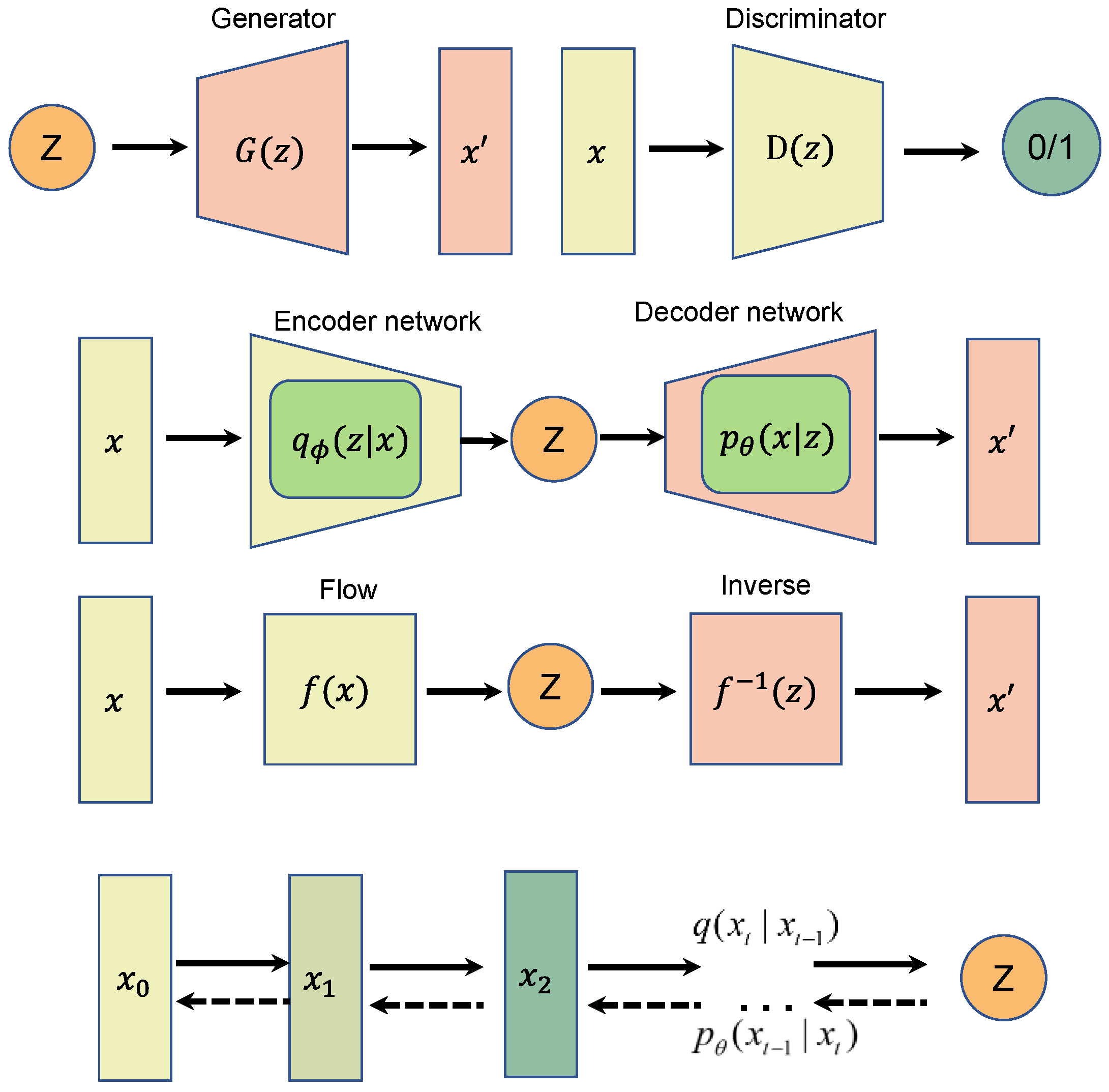
Comparison between the schematic diagrams of four generative models, from top to bottom: generative adversarial network (GAN), variational autoencoder (VAE), normalizing flow (NF), and diffusion model.
Remotesensing 15 03452 g001
Figure 2. The diffusion process and reverse diffusion process of the diffusion model used for image super-resolution.
Remotesensing 15 03452 g002
Figure 3. The primary components of the hybrid conditional diffusion model proposed for super-resolution of remote-sensing images.
Remotesensing 15 03452 g003
Figure 4. Framework of the proposed residual block with parameter (RBWP).
Remotesensing 15 03452 g004
Figure 5. The architecture of conditional noise predictor (U-Net).
Remotesensing 15 03452 g005
Figure 6. 
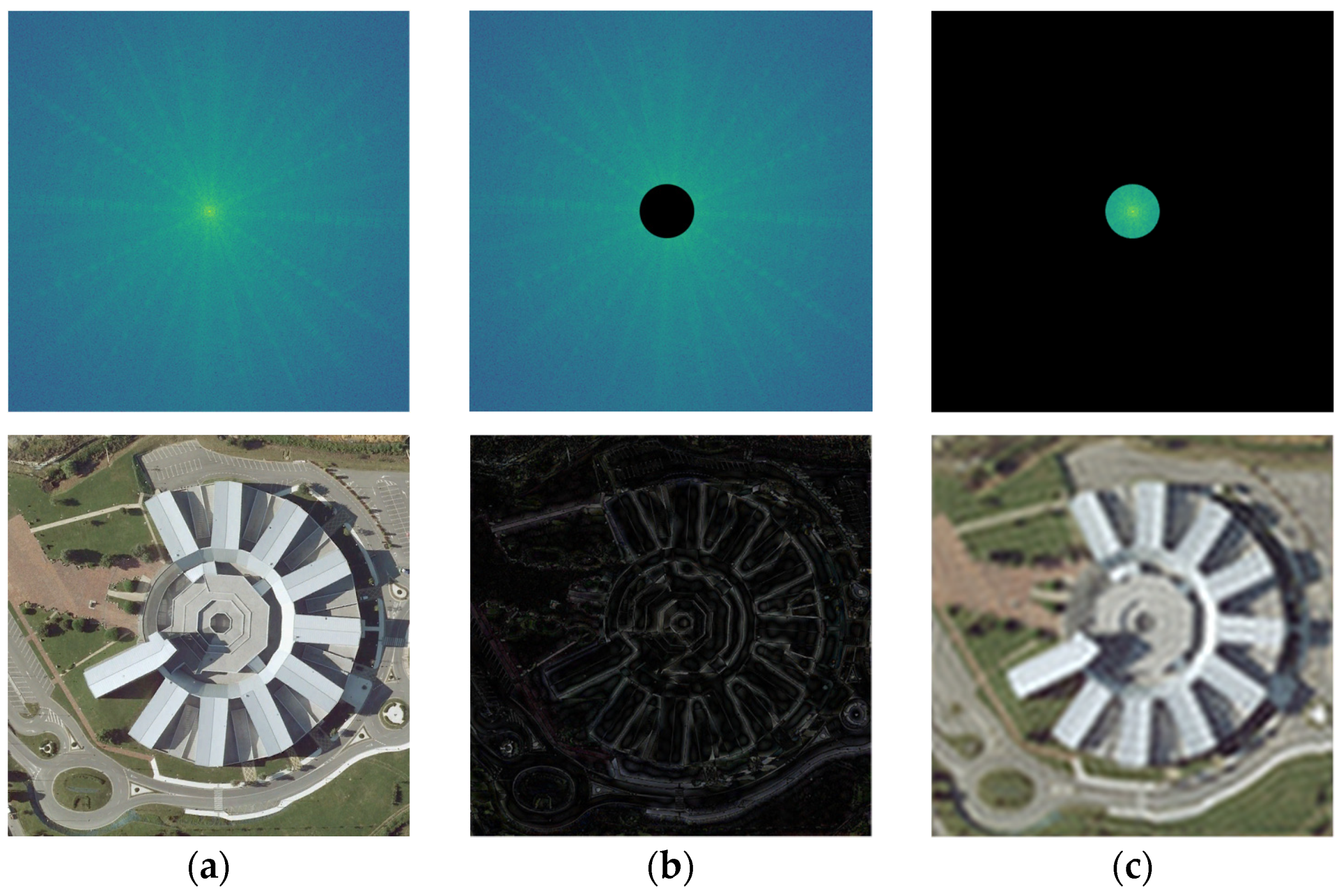
(a) The original image and its corresponding frequency spectrum, (b) the effect after applying a high-pass filter to the frequency spectrum, (c) the effect after applying a low-pass filter to the frequency spectrum.
Remotesensing 15 03452 g006
Figure 7. Schematic diagram of the high-frequency feature loss function.
Remotesensing 15 03452 g007
Figure 8. (af) depict the process of image reconstruction using the diffusion model, where the image on top represents x { 1 , , T } + u p ( x L R ) , and the image at the bottom represents x { 1 , , T } . (g) represents the result of the image reconstruction, where the image on top represents x 0 + u p ( x L R ) , and the image at the bottom represents x 0 .
Remotesensing 15 03452 g008
Figure 9. 
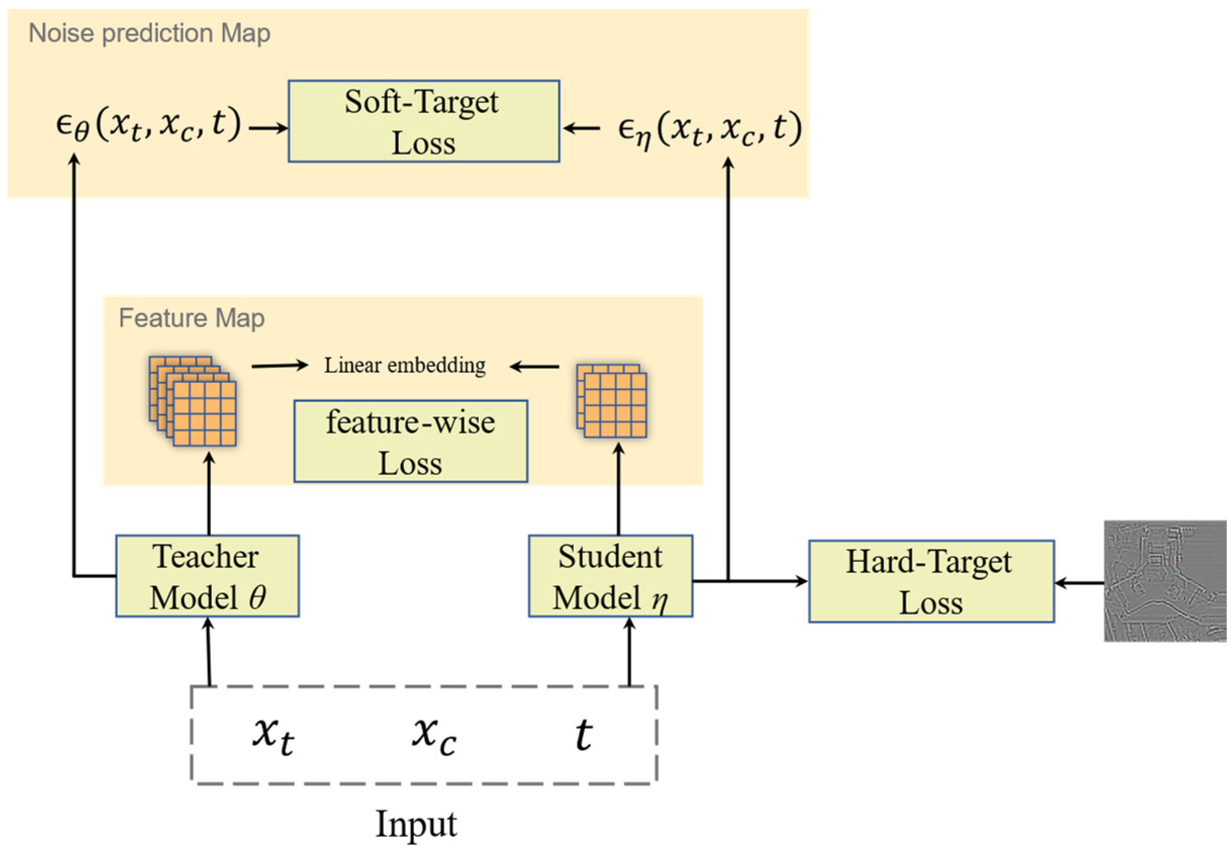
The feature distillation method applied to diffusion model super resolution.
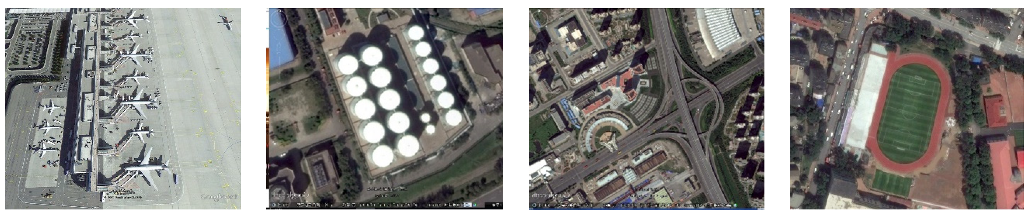
Remotesensing 15 03452 g009
Figure 10. 
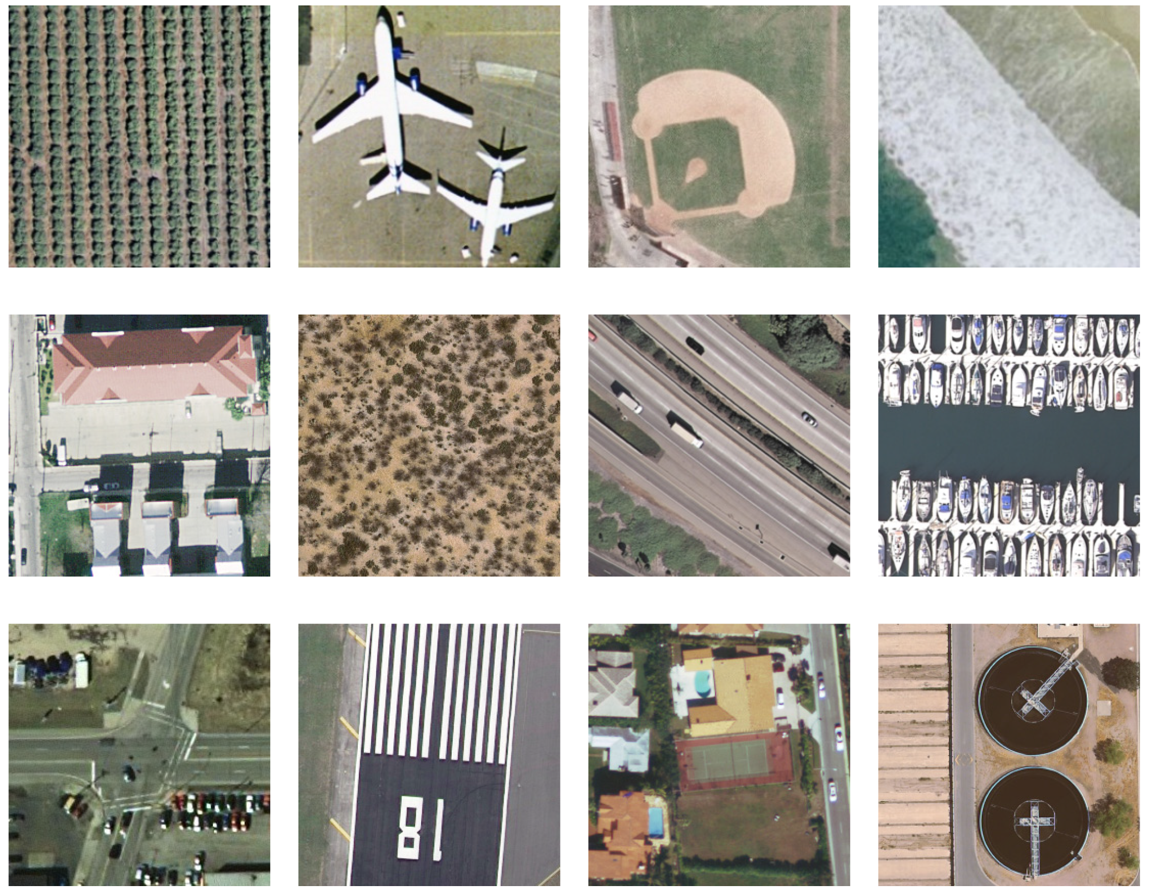
Display of images in different scene categories in the UC Merced Land Use test set.
Remotesensing 15 03452 g010
Figure 11. Display of images in different scene categories in the RSOD test set.
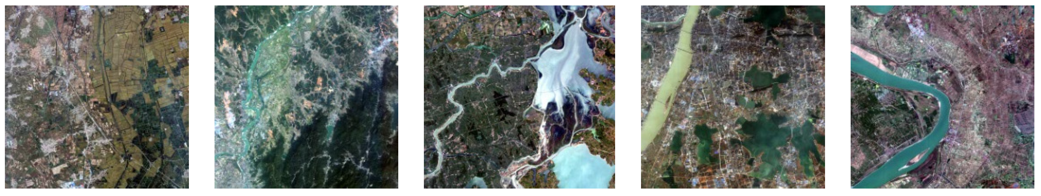
Remotesensing 15 03452 g011
Figure 12. Display of images in different scene categories in the Gaofen-2 test set.
Remotesensing 15 03452 g012
Figure 13. SR results at scale factor of ×4 on the test dataset [19,20] using different approaches (bj), and (a) represents the original high-resolution image for each approach.
Remotesensing 15 03452 g013aRemotesensing 15 03452 g013b
Figure 14. SR results at scale factor of ×8 on the test dataset [19,20] using different approaches (bj), and (a) represents the original high-resolution image for each approach.
Remotesensing 15 03452 g014aRemotesensing 15 03452 g014b
Figure 15. SR results at scale factor of ×2 on the real-world Gaofen-2 dataset [21] using different approaches (ad). (a) Bicubic; (b) SRCNN [5]; (c) MHAN [13]; (d) Ours.
Remotesensing 15 03452 g015
Figure 16. SR results at scale factor of ×4 on the real-world Gaofen-2 dataset [21] using different approaches (ad). (a) Bicubic; (b) SRCNN; (c) MHAN; (d) Ours.
Remotesensing 15 03452 g016aRemotesensing 15 03452 g016b
Figure 17. The visual quality comparison between the original model and the compressed model with a scale factor of ×4. (a) Ground truth; (b) Bicubic; (c) Original; (d) Distillation.
Remotesensing 15 03452 g017
Table 1. Comparison between different remote-sensing image super-resolution methods on the UCMerced_Land test dataset, with evaluation metrics including PSNR and SSIM values, at scale factors of ×2, ×4, and ×8.
Method×2×4×8
PSNR/SSIMPSNR/SSIMPSNR/SSIM
Bicubic30.55/0.89025.37/0.69822.15/0.481
SRCNN [5]32.20/0.91726.35/0.73022.52/0.515
VDSR [9]33.22/0.92527.02/0.76423.01/0.534
SAN [12]33.61/0.93427.42/0.77523.21/0.540
DDBPN [23]33.67/0.93127.49/0.77123.54/0.571
RDN [13]33.69/0.93327.54/0.78123.52/0.567
MHAN [10]33.61/0.92727.40/0.76423.56/0.559
EEGAN [28]33.54/0.92627.30/0.77023.44/0.553
Ours33.76/0.93027.60/0.78823.68/0.581
Table 2. Comparison between different remote-sensing image super-resolution methods on the RSOD test dataset, with evaluation metrics including PSNR and SSIM values, at scale factors of ×2, ×4, and ×8.
Method×2×4×8
PSNR/SSIMPSNR/SSIMPSNR/SSIM
Bicubic29.91/0.94226.71/0.80724.21/0.638
SRCNN [5]30.42/0.95127.22/0.83424.55/0.656
VDSR [9]30.87/0.96027.53/0.85924.89/0.673
SAN [12]31.08/0.96127.74/0.86525.08/0.694
DDBPN [23]31.13/0.96427.76/0.87225.10/0.703
RDN [13]31.16/0.96327.80/0.87125.13/0.704
MHAN [10]31.18/0.96727.71/0.86225.19/0.696
EEGAN [28]31.19/0.97327.69/0.86325.20/0.702
Ours31.16/0.96827.86/0.87625.33/0.710
Table 3. Performance comparison between different remote-sensing image super-resolution methods on the UCMerced_Land test dataset for various scenes at scale factor of ×2, with evaluation metrics including PSNR and SSIM values.
SceneSRCNN [5]VDSR [9]SAN [12]DDBPN [23]RDN [13]MHAN [13]EEGAN [28]Ours
PSNR/SSIM
Agricultural32.14/0.83132.18/0.83132.31/0.82932.22/0.82932.33/0.82632.25/0.83232.14/0.82732.32/0.829
Airplane32.96/0.92434.46/0.93934.89/0.94335.01/0.94435.10/0.94434.10/0.93334.86/0.94335.20/0.949
Baseball diamond35.33/0.89235.84/0.89936.19/0.90236.22/0.90236.25/0.90336.28/0.90136.14/0.90236.24/0.901
Beach38.58/0.95839.08/0.96339.33/0.96539.36/0.96539.38/0.96539.34/0.96339.33/0.96539.38/0.963
Buildings31.98/0.91633.39/0.93133.94/0.93533.99/0.93534.01/0.93633.93/0.92833.88/0.93434.10/0.938
Chaparral30.43/0.92930.86/0.93630.96/0.93731.01/0.93731.05/0.93830.94/0.93430.97/0.93731.01/0.934
Dense residential32.72/0.94334.10/0.95634.58/0.95934.64/0.95934.79/0.96134.54/0.95134.42/0.95834.75/0.966
Forest33.46/0.90733.88/0.91434.05/0.91534.04/0.91534.09/0.91633.97/0.91234.01/0.91534.11/0.916
Freeway33.68/0.94235.82/0.95936.34/0.96136.45/0.96236.51/0.96336.47/0.96536.17/0.96136.50/0.963
Golf course35.86/0.90236.31/0.90936.53/0.91336.55/0.91336.57/0.91336.56/0.91436.47/0.91236.58/0.913
Harbor29.58/0.95531.42/0.9732.24/0.97432.36/0.97432.54/0.97532.48/0.97632.21/0.97332.50/0.971
Intersection33.59/0.93434.58/0.94435.01/0.94835.11/0.94935.17/0.95035.19/0.95234.92/0.94835.22/0.953
Medium residential29.10/0.89330.06/0.90930.35/0.91330.41/0.91430.51/0.91430.58/0.91630.30/0.91330.49/0.911
Mobile home park28.82/0.91130.05/0.92830.45/0.93230.53/0.93330.59/0.93430.59/0.93630.39/0.93230.55/0.933
Overpass31.03/0.91433.01/0.93533.59/0.94033.77/0.94133.72/0.94133.74/0.94533.65/0.94033.78/0.941
Parking lot27.46/0.91828.56/0.93529.15/0.94029.28/0.94129.41/0.94229.36/0.94629.09/0.94029.40/0.944
River29.87/0.87330.21/0.88330.32/0.88630.34/0.88630.35/0.88730.31/0.88930.32/0.88630.33/0.884
Runway33.08/0.91634.54/0.93135.22/0.93635.28/0.93735.44/0.93835.45/0.94135.21/0.93535.46/0.938
Sparse residential31.12/0.88131.6/0.88931.75/0.89231.77/0.89231.81/0.89331.85/0.89431.73/0.89231.83/0.891
Storage tanks32.05/0.91333.24/0.92933.68/0.93333.74/0.93433.77/0.93434.77/0.93633.63/0.93333.80/0.930
Tennis court33.70/0.92935.06/0.94435.51/0.94835.55/0.94835.63/0.94935.53/0.94435.43/0.94735.66/0.952
Table 4. Performance comparison between different remote-sensing image super-resolution methods on the RSOD test dataset for various scenes at scale factor of ×2, with evaluation metrics including PSNR and SSIM values.
ScenesSRCNN [5]VDSR [9]SAN [12]DDBPN [23]RDN [13]MHAN [13]EEGAN [28]Ours
PSNR/SSIM
Aircraft34.67/0.96335.23/0.96835.34/0.96935.41/0.97135.40/0.97035.45/0.97235.48/0.97035.52/0.973
Oil tank29.69/0.97430.05/0.97730.22/0.97730.27/0.97930.27/0.97930.30/0.97930.34/0.98030.38/0.982
Overpass28.64/0.93229.07/0.93929.14/0.94029.27/0.94229.25/0.94229.33/0.94329.35/0.94329.35/0.945
Playground28.67/0.95329.14/0.95929.30/0.96029.37/0.96229.34/0.96229.43/0.96329.45/0.96329.44/0.963
Table 5. Performance comparison between different remote-sensing image super-resolution methods on the UCMerced_Land test dataset for various scenes at scale factor of ×4, with evaluation metrics including PSNR and SSIM values.
SceneSRCNN [5]VDSR [9]SAN [12]DDBPN [23]RDN [13]MHAN [13]EEGAN [28]Ours
PSNR/SSIM
Agricultural25.95/0.48925.95/0.49626.25/0.50626.26/0.50626.38/0.50826.27/0.50526.16/0.50326.45/0.506
Airplane26.76/0.77827.98/0.80828.52/0.81828.68/0.82128.69/0.82227.96/0.80528.45/0.81628.72/0.818
Baseball diamond30.71/0.75831.17/0.77031.47/0.77731.51/0.77831.55/0.77931.17/0.77031.34/0.77531.57/0.777
Beach32.64/0.85033.05/0.86333.20/0.86733.21/0.86733.23/0.86833.02/0.86333.17/0.86633.20/0.867
Buildings25.28/0.75726.41/0.79427.05/0.80827.05/0.81027.19/0.81226.54/0.79526.80/0.80327.45/0.808
Chaparral24.64/0.73624.99/0.75625.23/0.76725.28/0.76925.34/0.77225.04/0.75925.20/0.76525.43/0.767
Dense residential25.38/0.78326.32/0.82126.85/0.83526.95/0.83927.04/0.84126.37/0.82026.70/0.83226.95/0.837
Forest27.59/0.69227.77/0.70627.90/0.71327.90/0.71327.92/0.71527.78/0.70727.85/0.71128.07/0.716
Freeway27.40/0.80228.63/0.83729.38/0.85129.53/0.85529.58/0.85628.66/0.83629.22/0.8529.58/0.851
Golf course31.65/0.78231.99/0.79032.23/0.79632.26/0.79732.30/0.79831.97/0.79032.18/0.79532.23/0.796
Harbor21.52/0.78422.35/0.82122.92/0.83722.89/0.83923.01/0.84222.51/0.82122.67/0.82923.12/0.847
Intersection26.66/0.77027.32/0.79127.72/0.80327.82/0.80627.92/0.80827.45/0.79227.63/0.80128.05/0.814
Medium residential23.66/0.67724.29/0.70924.65/0.72324.73/0.72624.76/0.72724.30/0.70724.53/0.71824.85/0.723
Mobile home park23.07/0.72523.73/0.75924.11/0.77324.20/0.77724.22/0.77823.77/0.75924.02/0.76924.33/0.780
Overpass25.40/0.72426.39/0.76227.14/0.78927.26/0.79127.31/0.79426.47/0.76626.88/0.77927.34/0.789
Parking lot20.76/0.70721.16/0.73921.50/0.75221.60/0.75321.63/0.75421.23/0.73721.39/0.74721.68/0.758
River25.61/0.65625.88/0.67626.04/0.68626.05/0.68726.06/0.68825.9/0.67726.01/0.68426.04/0.693
Runway27.53/0.77729.41/0.81930.19/0.83030.45/0.83330.38/0.83429.54/0.81630.04/0.82830.39/0.841
Sparse residential26.47/0.68026.83/0.69927.04/0.70627.07/0.70827.08/0.70926.85/0.69926.98/0.70527.04/0.706
Storage tanks26.43/0.74127.14/0.77327.64/0.79027.72/0.79327.78/0.79527.23/0.77527.52/0.78527.74/0.790
Tennis court27.83/0.76628.49/0.79029.01/0.80729.14/0.81129.18/0.81328.55/0.79128.85/0.80229.21/0.807
Table 6. Performance comparison between different remote-sensing image super-resolution methods on the RSOD test dataset for various scenes at scale factor of ×4, with evaluation metrics including PSNR and SSIM values.
SceneSRCNN [5]VDSR [9]SAN [12]DDBPN [23]RDN [13]MHAN [13]EEGAN [28]Ours
PSNR/SSIM
Aircraft30.23/0.86930.84/0.88430.92/0.88731.16/0.89231.06/0.89031.20/0.89331.25/0.89431.30/0.896
Oil tank27.52/0.90527.65/0.91427.74/0.91827.82/0.92327.77/0.92027.82/0.92227.86/0.92427.89/0.928
Overpass25.25/0.74625.5/0.76825.55/0.77125.66/0.7825.63/0.77825.68/0.78225.71/0.78325.80/0.788
Playground25.88/0.83526.15/0.85326.29/0.85626.32/0.86326.28/0.86126.34/0.86426.37/0.86626.46/0.872
Table 7. Performance comparison between different remote-sensing image super-resolution methods on the UCMerced_Land test dataset for various scenes at scale factor of ×8, with evaluation metrics including PSNR and SSIM values.
SceneSRCNN [5]VDSR [9]SAN [12]DDBPN [23]RDN [13]MHAN [13]EEGAN [28]Ours
PSNR/SSIM
Agricultural23.34/0.26623.38/0.27623.36/0.27723.53/0.29623.46/0.29123.46/0.29823.32/0.29423.60/0.316
Airplane22.22/0.59423.13/0.63723.44/0.63824.09/0.66924.02/0.66424.01/0.66823.95/0.66324.22/0.672
Baseball diamond27.26/0.61927.81/0.63628.00/0.64128.30/0.65128.28/0.65328.22/0.64128.14/0.63928.39/0.662
Beach29.29/0.72529.72/0.73729.84/0.74029.98/0.74629.97/0.74529.96/0.74229.88/0.74030.06/0.763
Buildings20.53/0.51621.51/0.57021.86/0.5822.47/0.61722.44/0.61222.44/0.58822.36/0.57222.52/0.628
Chaparral20.47/0.35020.54/0.37020.59/0.37720.67/0.38820.69/0.39020.63/0.38220.51/0.37720.75/0.394
Dense residential20.50/0.51221.21/0.56421.42/0.56721.87/0.60421.86/0.60121.84/0.59221.77/0.59621.92/0.613
Forest24.62/0.43524.72/0.45024.78/0.45424.83/0.46224.84/0.46324.87/0.46624.74/0.46124.91/0.471
Freeway23.07/0.52723.57/0.55524.02/0.60124.57/0.64124.48/0.64124.46/0.63624.38/0.63124.64/0.653
Golf course27.98/0.66228.78/0.68128.96/0.68329.33/0.69329.27/0.69129.23/0.69429.11/0.69629.46/0.697
Harbor17.07/0.52717.37/0.56317.61/0.57517.85/0.60717.89/0.60617.84/0.59417.70/0.59517.96/0.617
Intersection22.43/0.53022.88/0.55823.12/0.56623.43/0.58923.44/0.58723.42/0.58823.35/0.58723.58/0.595
Medium residential20.29/0.42420.73/0.45720.89/0.46321.19/0.49121.17/0.48821.12/0.48821.08/0.48321.25/0.495
Mobile home park18.91/0.45719.31/0.49119.56/0.50119.89/0.53419.88/0.52919.82/0.52919.78/0.52219.94/0.538
Overpass22.01/0.48222.62/0.51622.84/0.52623.37/0.55823.26/0.55623.27/0.55523.16/0.55423.48/0.562
Parking lot17.01/0.40317.21/0.43417.27/0.43617.36/0.46317.36/0.45917.31/0.45517.27/0.45817.44/0.461
River23.36/0.47523.60/0.49223.70/0.49723.85/0.50923.84/0.50823.86/0.50123.72/0.49623.96/0.519
Runway22.70/0.58523.67/0.62124.33/0.63425.07/0.65925.12/0.65825.16/0.65025.05/0.65325.14/0.670
Sparse residential23.15/0.45623.51/0.47723.67/0.48223.80/0.49523.82/0.49423.88/0.49123.77/0.49523.94/0.496
Storage tanks23.12/0.55123.53/0.57623.66/0.58123.98/0.60223.93/0.59823.91/0.59623.80/0.58924.06/0.612
Tennis court23.91/0.57024.42/0.59724.63/0.60225.04/0.62825.01/0.62325.05/0.62725.02/0.62525.13/0.637
Table 8. Performance comparison between different remote-sensing image super-resolution methods on the RSOD test dataset for various scenes at scale factor of ×8, with evaluation metrics including PSNR and SSIM values.
ScenesSRCNN [5]VDSR [9]SAN [12]DDBPN [23]RDN [13]MHAN [13]EEGAN [28]Ours
PSNR/SSIM
Aircraft26.67/0.73827.25/0.75627.51/0.76427.46/0.76127.61/0.76827.71/0.77227.70/0.77227.81/0.779
Oil tank25.18/0.73925.43/0.75325.73/0.77025.69/0.76825.77/0.77125.80/0.77625.76/0.77725.89/0.786
Overpass22.72/0.50822.97/0.53123.12/0.54523.11/0.54223.10/0.54523.25/0.55823.26/0.55923.30/0.561
Playground23.62/0.65123.89/0.67324.07/0.68524.05/0.68224.06/0.68824.18/0.69524.20/0.69624.27/0.704
Table 9. Comparison between original model and compressed model in terms of parameters, computation, and time consumption. The size of the input image was 256 × 256 pixels, with a scale factor of ×4.
Model Params   ( 10 6 ) GFLOPsTime (ms) *
Original9.0745.2856
Distillation4.5222.6463
* The reverse diffusion process consumes time.
Table 10. The comparison between quantitative results of the original model and the compressed model on the RSOD test dataset.
RSOD×2×4×8
PSNR/SSIMPSNR/SSIMPSNR/SSIM
Original31.16/0.96827.86/0.87625.33/0.710
Distillation31.10/0.96127.24/0.86525.27/0.704
Table 11. Comparison between the time consumptions of different super-resolution algorithms during the model inference process. The size of the input image was 256 × 256 pixels, with a scale factor of ×4.
ModelSRCNNVDSRRDNMHANSANDDBPNEEGANOurs
Time (ms) *1.73.01614.817.336.927.5463
* The time consumed during the inference process of the model.
Table 12. This paper investigated the impact of different module combinations in the proposed hybrid conditional diffusion model on the super-resolution performance of remote-sensing images. All experiments were conducted on the UCMerced_Land test dataset.
DescriptionDifferent Types of Combinations
Module123456
Hybrid conditional featureTransformer network
CNN
Fourier high-frequency spatial constraint
×2PSNR33.1633.1833. 2533.4733.5933.76
SSIM0.9160.9180.9220.9130.9210.930
×4PSNR27.2827.3727.4827.4427.5227.60
SSIM0.7640.7650.7710.7710.7820.788
×8PSNR23.3423.3723.3623.5023.5723.68
SSIM0.5480.5500.5510.5720.5710.581
Disclaimer/Publisher’s Note: The statements, opinions and data contained in all publications are solely those of the individual author(s) and contributor(s) and not of MDPI and/or the editor(s). MDPI and/or the editor(s) disclaim responsibility for any injury to people or property resulting from any ideas, methods, instructions or products referred to in the content.

