Article

Hybrid-Scale Hierarchical Transformer for Remote Sensing Image Super-Resolution

1
School of Electrical and Electronic Engineering, Shandong University of Technology, Zibo 255000, China
2
School of Electronic Engineering and Computer Science, Queen Mary University of London, London E1 4NS, UK
3
Department of Embedded Systems Engineering, Incheon National University, Incheon 22012, Republic of Korea
*
Author to whom correspondence should be addressed.
Remote Sens. 2023, 15(13), 3442; https://doi.org/10.3390/rs15133442
Submission received: 19 April 2023 / Revised: 21 June 2023 / Accepted: 30 June 2023 / Published: 7 July 2023

Abstract

:
Super-resolution (SR) technology plays a crucial role in improving the spatial resolution of remote sensing images so as to overcome the physical limitations of spaceborne imaging systems. Although deep convolutional neural networks have achieved promising results, most of them overlook the advantage of self-similarity information across different scales and high-dimensional features after the upsampling layers. To address the problem, we propose a hybrid-scale hierarchical transformer network (HSTNet) to achieve faithful remote sensing image SR. Specifically, we propose a hybrid-scale feature exploitation module to leverage the internal recursive information in single and cross scales within the images. To fully leverage the high-dimensional features and enhance discrimination, we designed a cross-scale enhancement transformer to capture long-range dependencies and efficiently calculate the relevance between high-dimension and low-dimension features. The proposed HSTNet achieves the best result in PSNR and SSIM with the UCMecred dataset and AID dataset. Comparative experiments demonstrate the effectiveness of the proposed methods and prove that the HSTNet outperforms the state-of-the-art competitors both in quantitative and qualitative evaluations.

1. Introduction

With the rapid progress of satellite platforms and optical remote sensing technology, remote sensing images (RSIs) have been broadly deployed in civilian and military fields, e.g., disaster prevention, meteorological forecast, military mapping, and missile warning [1,2]. However, due to hardware limitations and environmental restrictions [3,4], RSIs often suffer from low-resolution (LR) and contain some intrinsic noise. Upgrading physical imaging equipment to improve resolution is often plagued by high costs and long development cycles. Therefore, it is of utmost urgency to explore the remote sensing image super-resolution (RSISR).
Single-image super-resolution (SR) is a highly ill-posed visual problem which aims to reconstruct high-resolution (HR) images from corresponding degraded LR images. To this end, many representative algorithms have been proposed, which can be roughly divided into three categories, i.e., interpolation-based methods [5,6], reconstruction-based methods [7,8], and learning-based methods [9,10]. The interpolation-based methods generally utilize different interpolation operations, including bilinear interpolation, bicubic interpolation, and nearest interpolation, to estimate unknown pixel value [11]. These methods are relatively straightforward in practice, while the reconstructed images lack essential details. In contrast, reconstruction-based methods improve image quality by incorporating prior information of the image as constraints into the HR image. These methods can restore high-frequency details with the help of prior knowledge, while they require substantial computational costs, making it difficult for them to be readily applied to RSIs [12]. Learning-based approaches try to produce HR images by learning the mapping relationship established between external LR–HR image training pairs. Compared with the aforementioned two lines of methods, learning-based methods achieve better performance and become the mainstream in this domain due to the powerful feature representation ability provided by convolutional neural networks (CNNs) [13]. However, learning-based methods generally adopt the post-upsampling framework [14], which solely exploits low-dimensional features while ignoring the discriminative high-dimensional feature information after the upsampling process.
In addition to utilizing nonlinear mapping between LR–HR image training pairs, the self-similarity of the image is also employed to improve the performance of SR algorithms. Self-similarity refers to the property of similar patches appear repeatedly in a single image and is broadly adopted in image denoising [15,16], deblurring [17], and SR [18,19,20]. Self-similarities are also an intrinsic property in RSIs, i.e., internal recursive information. Figure 1 illustrates the self-similarities in RSIs. One can see that the down-scaled image is on the left, and the original one is on the right. Similar highway patches with green box labels appear repeatedly in the same scale image, while the roof of factories with red box labels appear repeatedly across different scales, and these patches with similar edges and textures contain abundant internal recursive information. Previously, Pan et al. [21] employed dictionary learning to capture structural self-similarity features as additional information to improve the performance of the model. However, the sparse representation of SR has a limited ability to leverage the internal recursive information within the entire remote sensing image.
In this paper, we propose a Hybrid-Scale Hierarchical Transformer Network (HSTNet) for RSISR. The HSTNet can enhance the representation of the high-dimensional features after upsampling layers and fully utilize the self-similarity information in RSIs. Specifically, we propose a hybrid-scale feature exploitation (HSFE) module to leverage the internal similar information both in single and cross scales within the images. The HSFE module contains two branches, i.e., a single-scale branch and a cross-scale branch. The former is employed to capture the recurrence within the same scale image, and the latter is utilized to learn the feature correlation across different scales. Moreover, we designed a cross-scale enhancement transformer (CSET) module to capture long-range dependencies and efficiently model the relevance between high-dimension and low-dimension features. In the CSET module, the encoders are used to encode low-dimension features from the HSFE module, and the decoder is used to utilize to fuse the multiple hierarchies high-/low-dimensional features so as to enhance the representation ability of high-dimensional features. To sum up, the main contributions of this work are as follows:
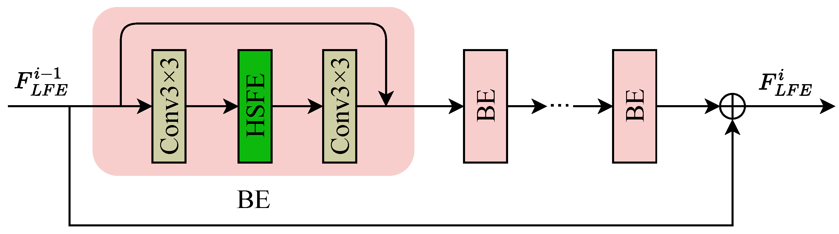
  • We propose an HSFE module with two branches to leverage the internal recursive information from both single and cross scales within the images for enriching the feature representations for RSISR.
  • We designed a CSET module to capture long-range dependencies and efficiently calculate the relevance between high-dimension and low-dimension features. It helps the network reconstruct SR images with rich edges and contours.
  • Jointly incorporating the HSFE and CSET modules, we formed the HSTNet for RSISR. Extensive experiments on two challenging remote sensing datasets verify the superiority of the proposed model.

2. Related Literature

2.1. CNN-Based SR Models

Dong et al. [22] pioneered the adoption of an SR convolutional neural network (SRCNN) that utilizes three convolution layers to establish the nonlinear mapping relationship between LR–HR image training pairs. On the basis of the residual network introduced by He et al. [23], Kim et al. [24] designed a very deep SR convolutional neural network (VDSR) where residual learning is employed to accelerate model training and improve reconstruction quality. Lim et al. [25] built the enhanced deep super-resolution model to simplify the network and improve the computational efficiency via optimizing the initial residual block. Zhang et al. [26] designed a deep residual dense network in which the residual network with dense skip connections is used to transfer intermediate features. Benefiting from the channel attention (CA) module, Zhang et al. [27] presented a deep residual channel attention network to enhance the high-frequency channel feature representation. Dai et al. [28] designed a second-order CA mechanism to guide the model to improve the ability of discriminative learning ability and exploit more conducive features. Li et al. [29] proposed an image super-resolution feedback network (SRFBN) in which a feedback mechanism is adopted to transfer high-level feature information. The SRFBN could leverage high-level features to polish up the representation of low-level features.
Because of the impact of spatial resolution on the final performance of many RSI tasks, including instance segmentation, object detection, and scene classification, RSISR also raises significant research interest. Lei et al. [30] proposed a local–global combined network (LGCNet) which can enhance the multilevel representations, including local detail features and global information. Haut et al. [31] produced a deep compendium model (DCM), which leverages skip connection and residual unit to exploit more informative features. To fuse different hierarchical contextual features efficiently, Wang et al. [32] designed a contextual transformation network (CTNet) based on a contextual transformation layer and contextual feature aggregation module. Ni et al. [33] designed a hierarchical feature aggregation and self-learning network in which both self-learning and feedback mechanisms are employed to improve the quality of reconstruction images. Wang et al. [34] produced a multiscale fast Fourier transform (FFT)-based attention network (MSFFTAN), which employs a multi-input U-shape structure as the backbone for accurate RSISR. Liang et al. [35] presented a multiscale hybrid attention graph convolution neural network for RSISR in which a hybrid attention mechanism was adopted to obtain more abundant critical high-frequency information. Wang et al. [36] proposed a multiscale enhancement network which utilizes multiscale features of RSIs to recover more high-frequency details. However, the CNN-based methods above generally employ the post-upsampling framework that directly recovers HR images after the upsampling layer, ignoring the discriminative high-dimensional feature information after the upsampling process [14].

2.2. Transformer-Based SR Models

Due to the strong long-range dependence learning ability of transformers, transformer-based image SR methods have been studied recently by many scientific researchers. Yang et al. [37] produced a texture transformer network for image super-resolution, in which a learnable texture extractor is utilized to exploit and transmit the relevant textures to LR images. Liang et al. [38] proposed SwinIR by transferring the ability of the Swin Transformer, which could achieve competitive performance on three representative tasks, namely image denoising, JPEG compression artifact reduction, and image SR. Fang et al. [39] designed a lightweight hybrid network of a CNN and transformer that can extract beneficial features for image SR with the help of local and non-local priors. Lu et al. [40] presented a hybrid model with a CNN backbone and transformer backbone, namely the efficient super-resolution transformer, which achieved impressive results with low computational cost. Yoo et al. [41] introduced an enriched CNN–transformer feature aggregation network in which the CNN branch and transformer branch can mutually enhance each representation during the feature extraction process. Due to the limited ability of multi-head self-attention to extract cross-scale information, cross-token attention is adopted in the transformer branch to utilize information from tokens of different scales.
Recently, transformers have also found their way into the domain of RSISR. Lei et al. [14] proposed a transformer-based enhancement network (TransENet) to capture features from different stages and adopted a multistage-enhanced structure that can integrate features from different dimensions. Ye et al. [42] proposed a transformer-based super-resolution method for RSIs, and they employed self-attention to establish dependencies relationships within local and global features. Tu et al. [43] presented a GAN that draws on the strengths of the CNN and Swin Transformer, termed the SWCGAN. The SWCGAN fully considers the characteristics of large size, a large amount of information, and a strong relevance between pixels required for RSISR. He et al. [44] designed a dense spectral transformer to extract the long-range dependence for spectral super-resolution. Although the transformer can improve the long-range dependence learning ability of the model, these methods do not leverage the self-similarity within the entire remote sensing image [45].

3. Methodology

3.1. Overall Framework

The framework of the proposed HSTNet is shown in Figure 2. It is built by the combination of three kinds of fundamental modules, i.e., a low-dimension feature extraction (LFE) module, a cross-scale enhancement transformer (CSET) module, and an upsample module. Specifically, the LFE module is utilized to extract high-frequency features across different scales, and the CSET module is employed to capture long-range dependency to enhance the final feature representation. The upsample module is adopted to transform the feature representation from a low-dimensional space to a high-dimensional space.
Given an LR image I LR , a convolutional layer with a 3 × 3 kernel is utilized to extract the initial feature F 0 . The process of shallow feature extraction is formulated as
F 0 = f sf I LR ,
where f sf · represents the operation of the convolutional operation and F 0 is the shallow feature.
As shown in Figure 3, the LFE module consists of five basic extraction (BE) modules, and each BE module contains two 3 × 3 convolution layers and one hybrid-scale feature exploitation (HSFE) module. As the core component of the BE module, the HSFE module is proposed to model image self-similarity. The whole low-dimensional feature extraction process is formulated as
F LFE i = f lfe i F LFE i 1 = f lfe i f lfe i 1 f lfe 1 F 0 , i = 1 , 2 , 3 ,
where f lfe i · and F LFE i represent the operation of ith LFE module and its output. After the three cascaded LFE modules, a subpixel layer [46] is adopted to transform low-dimensional features into high-dimensional features, which is formulated as
F up = Subpixel F LFE 3 ,
where F up represents the high-dimension feature and Subpixel · denotes the function of the subpixel layer. The low-dimension features F LFE 1 , F LFE 2 , and F LFE 3 and the high-dimension feature F up are fed into three cascaded CSET modules for feature hierarchical enhancement. To reduce the redundancy of the enhanced features, a 1 × 1 convolution layer is employed to reduce the feature dimension. The complete process including the enhancement and dimension reduction is formulated as
F C S E T i = f cset i F LFE i , F CSET i + 1 , i = 1 , 2 , f cset i F LFE i , F up , i = 3 ,
where f cset i · and F CSET i represent the operation of ith CSET module and its output, respectively. Finally, one convolution layer is employed to obtain SR image I SR from the enhanced features. A conventional L 1 loss function was employed to train the proposed HSTNet model. Given a training set I LR i , I HR i i = 1 N , the loss function is formulated as:
L θ = 1 N i = 1 N F HSTNet I LR i I HR i 1 ,
where F HSTNet denotes the proposed model parameterized by θ and N represents the number of training LR–HR pairs.

3.2. Hybrid-Scale Feature Exploitation Module

To explore the internal recursive information in single-scale and cross-scale, we propose an HSFE module. Figure 4 exhibits the architecture of the HSFE module, which consists of a single-scale branch and a cross-scale branch. The single-scale branch aims to capture similar features within the same scale, and a non-local (NL) block [47] was utilized to calculate the relevance of these features. The cross-scale branch was applied to capture recursive features of the same image at different scales, and an adjusted non-local (ANL) block [45] was utilized to calculate the relevance of features between two different scales.
Single-scale branch: As depicted in Figure 4, we built the single-scale branch to extract single-scale features. Specifically, in the single-scale branch, several convolutional layers are applied to capture recursive features, and an NL block is employed to guide the network to concentrate on informative areas. As shown in Figure 4a, an embedding function is utilized to mine the similarity information as
f x i , x j = e θ T x i φ x j = e W θ x i T W φ x j ,
where i is the index of the output position, j is the index that enumerates all positions, and x denotes the input of the NL block. W θ and W φ are the embeddings weight matrix. The non-local function is symbolized as
y i = j f x i , x j g x j / j f x i , x j .
The relevance between x i and all x j can be calculated by pairwise function f ( · ) . The feature representation of x j can be obtained by the function g ( · ) . Eventually, the output of the NL block is obtained by
z i = W ϕ y i + x i ,
where W ϕ is a weight matrix.
The convolution layer following the NL block transforms the input into an attention diagram, which is then normalized with a sigmoid function. In addition, the main branch output features are multiplied by the attention diagram, where the activation values for each space and channel location are rescaled.
Cross-scale branch: As depicted in Figure 4, the cross-scale branch is utilized to perform cross-scale feature representation. Specifically, the input of the HSFE module is considered the basic scale feature, which is symbolized as F i n b . To exploit the internal recursive information at different scales, the downsampled scale feature F i n d is formulated as
F i n d = f down s F i n b ,
where f down s ( · ) denotes the operation of downsampling with scale factor s.
Two contextual transformation layers (CTLs) [48] are employed to extract feature with two different scales F i n b and F i n d . To align the spatial dimension of the features in different scales, the downsampled feature is firstly upsampled with the scale factor of s. x b and x b represent the output of the basic scale and the downsampled scale through the two CTLs, and this process is formulated as
x b = f c t l F i n b x d = f u p s f c t l F i n b ,
where f c t l · denotes the operation of two CTLs and f u p s · represents the operation of upsample with scale factor s.
Similar to the single-scale branch, an ANL block [45] was introduced to exploit the feature correlation between two different scales RSIs. As shown in Figure 4b, the ANL block is improved compared to the NL block, and they have different inputs. Thus, z i in Equation (8) for ANL block can be rewritten as
f x i d , x j b = e θ T x i d φ x j b = e W θ x i d T W φ x j b ,
y i = j f x i d , x j b g x j b / j f x i b , x j d
z i = W ϕ y i + x i .
In the cross-scale branch, we employ the ANL block to fuse multiple scale features, therefore fully utilizing the self-similarity information. The HSFE module can be formulated as
F o u t = f s i n F i n + f c r o F i n + F i n ,
where F i n is the input of the HSFE module and F o u t is the output of the HSFE module. f s i n · and f c r o · are the operation of the single-scale branch and cross-scale branch, respectively.

3.3. Cross-Scale Enhancement Transformer Module

The cross-scale enhancement transformer module is designed to learn the dependency relationship across long distances between high-dimension and low-dimension features and enhance the final feature representation. The architecture of the CSET module is shown in Figure 5a. Specifically, we introduced the cross-scale token attention (CSTA) module [41] to exploit the internal recursive information within an input image across different scales. Moreover, we use three CSET modules to utilize different hierarchies of feature information. Figure 5a illustrates in detail the procedure of feature enhancement using CSET-3 module as an example.
Transformer encoder: The encoders are used to encode different hierarchies of features from LFE modules. As shown in Figure 5a, the encoder is mainly composed of a multi-headed self-attention (MHSA) block and a feed-forward network (FFN) block, which is similar to the original design in [49]. The FFN block contains two multilayer perceptron (MLP) layers with an expansion ratio r and a GELU activation function [50] in the middle. Moreover, we adopted layer normalization (LN) before the MHSA block and FFN block, and employed a local residual structure to avoid the gradient vanishing or explosion during gradient backpropagation. The entire process of the encoder can be formulated as
F E N i = f m h s a f l n F L F E i + F L F E i F E N i = f f f n f l n F E N i + F E N i ,
where f m h s a · , f l n · , and f f f n · denote the function of the MHSA block, layer normalization, and FFN block, respectively. F E N i is the intermediate output of the encoder. F L F E i and F E N i are the input and output of the encoder in the ith CSET module.
Transformer decoder: The decoders are utilized to fuse high-/low-dimensional features from multiple hierarchies to enhance the representation ability of high-dimensional features. As shown in Figure 5a, the decoder contains two MHSA blocks and a CSTA block [41]. With the CSTA block, the decoder can exploit the recursive information within an input image across different scales. The operation of the decoder can be formulated as
F D E i = f c s t a f l n F u p + F u p F D E i = f m h s a f l n F D E i , F E N i + F D E i F C S E T i = f m h s a f l n F D E i + F D E i
where f c s t a · denotes the process of the CSTA block and F u p is the output of Encoder-4. Each CSET module has two inputs, and the composition of the inputs is determined by the location of the CSET module. F D E i and F D E i represent the intermediate outputs of the decoder. F C S E T i represents the output of ith CSET module.
CSTA block: The CSTA block [41] is introduced to utilize the recurrent patch information of different scales in the input image. The feature information flow of the CSTA module is illustrated in Figure 5b. Specifically, the input token embeddings T R n × d of the CSTA block are split into T a R n × d 2 and T b R n × d 2 along the channel axis. Then, T s R n × d 2 including n tokens from T a and T l R n × d including n tokens by rearranging T b are generated. The number of tokens in T l can be set to n = h t s + 1 × w t s + 1 , where t and s represent the stride and token size. To improve efficiency, T s is replaced by T a , and T l is tokenized with a larger token size and overlapping. Numerous large-size tokens can be obtained by overlapping, enabling the transformer to actively learn patch recurrence across scales.
To effectively exploit self-similarity across different scales, we computed cross-scale attention scores between tokens in both T s and T l . Specifically, the queries q s R n × d 2 , keys k s R n × d 2 , and values v s R n × d 2 were generated from T s . Similarly, the queries q l R n × d 2 , keys k l R n × d 2 , and values v l R n × d 2 were generated from T l . The reorganized triples q s , k l , v l and q l , k s , v s were obtained by swapping their key–value pairs to each other. Then, the attention operation was executed using the reorganized triples. It should be noted that the projection of attention operations reduces the last dimension of queries, keys, and values in T l from d to d / 2 . Subsequently, we re-projected the attention results of T l to the dimension of n × d then transformed to the dimension of n × d 2 . Finally, we concatenated the attention results to obtain the output of the CSTA block.

4. Experiments

4.1. Experimental Dataset and Settings

We evaluate the proposed method on two widely adopted benchmarks [30,31,51], namely the UCMecred dataset [52] and AID dataset [53], to demonstrate the effectiveness of the proposed HSTNet.
UCMerced dataset: This dataset consists of 2100 images belonging to 21 categories of varied remote sensing image scenes. All images exhibit a pixel size of 256 × 256 and a spatial resolution of 0.3 m/pixel. The dataset is divided equally into two distinct sets, one comprising 1050 images for training and the other for testing.
AID dataset: This dataset encompasses 10,000 remote sensing images, spanning 30 unique categories. In contrast to the UCMerced dataset, all images in this dataset have a pixel size of 600 × 600 and spatial resolution of 0.5 m/pixel. A selection of 8000 images from this dataset was randomly chosen for the purpose of training, while the remaining 2000 images were used for testing. In addition, a validation set consisting of five arbitrary images from each category was established.
To verify the generalization of the proposed method, we further adapted the trained model to the real-world images of Gaofen-1 and Gaofen-2 satellites. We downsampled HR images through bicubic operations to obtain LR images. Two mainstream metrics, namely peak signal-to-noise ratio (PSNR) and structural similarity index measure (SSIM), were calculated on the Y channel of the YCbCr space for objective evaluation. They are formulated as
P S N R I S R , I H R = 10 · log 10 × L 2 1 N i = 1 N I S R i I H R i 2 ,
where L represents the maximum pixel, and N denotes the number of all pixels in I S R and I H R .
S S I M x , y = 2 u x u y + k 1 u x 2 + u y 2 + k 1 · σ x y + k 2 σ x 2 + σ y 2 + k 2 ,
where x and y represent two images. σ x y symbolizes the covariance between x and y. u and σ 2 represent the average value and variance. k 1 and k 2 denote constant relaxation terms. Multi-adds and model parameters were utilized to evaluate the computational complexity [32,54]. In addition, the natural image quality evaluator (NIQE) was adopted to validate the reconstruction of real-world images from Gaofen-1 and Gaofen-2 satellites [55].

4.2. Implementation Details

We conducted experiments on remote sensing image data with scale factors of × 2 , × 3 , and × 4 . During training, we randomly cropped 48 × 48 patches from LR images and extracted ground-truth references from corresponding HR images. We also employed horizontal flipping and random rotation (90°, 180° and 270°) to augment training samples. Table 1 presents the comprehensive hyperparameter setting of the cross-scale enhancement transformer (CSET) module.
We adopted the Adam optimizer [56] to train the HSTNet with β 1 = 0.9, β 2 = 0.99, and ϵ = 10 8 . The initial learning rate was set to 10 4 , and the batch size was 16. The proposed model was trained for 800 epochs, and the learning rate decreased by half after 400 epochs. Both the training and testing stages were performed using the PyTorch framework, utilizing CUDAToolkit 11.4, cuDNN 8.2.2, Python 3.7, and two NVIDIA 3090 Ti GPUs.

4.3. Comparison with Other Methods

To verify the effectiveness of the proposed HSTNet, we conducted comparative experiments with some state-of-the-art (SOTA) competitors, namely SC [12], SRCNN [22], FSRCNN [57], VDSR [24], LGCNet [30], DCM [31], CTNet [48], ESRT [40], ACT [41], and TransENet [14]. Among these methods, SC [12], SRCNN [22], FSRCNN [57], VDSR [24], ESRT [40], and ACT [41] are the methods proposed for natural image SR. LGCNet [30], DCM [31], CTNet [48], and TransENet [14] are designed for RSISR. The experimental results for the UCMerced dataset and AID dataset with the scale factors of × 2 , × 3 and × 4 are reported in Table 2.

4.3.1. Quantitative Evaluation

Evaluation with UCMerced dataset: Table 2 shows that the proposed HSTNet achieves first place among competitors for the UCMerced dataset for all scale factors. Specifically, the HSTNet improves the PSNR comparatively by 0.71 dB, 0.54 dB, and 0.60 dB for scale factor × 2 for LGCNet [30], DCM [31] and CTNet [48], respectively. The average PSNR values of the proposed HSTNet over the second-best TransENet that employs a transformer module are 0.16 dB, 0.15 dB and 0.12 dB when the scale factors are × 2 , × 3 and × 4 , respectively. Additionally, the HSTNet outperforms LGCNet [30], DCM [31], and CTNet [48] in terms of SSIM by 0.0183, 0.0027, and 0.0102 for scale factor × 3 . Compared to ACT [41], which also uses a transformer structure, the average PSNR obtained by the proposed method increased by 0.31 dB, 0.27 dB, and 0.35 dB at scale factors of × 2 , × 3 and × 4 , respectively. Moreover, Table 3 lists the mean PSNR of different methods on all 21 classes (All these 21 classes of UCMerced dataset: 1—Agricultural, 2—Airplane, 3—Baseballdiamond, 4—Beach, 5—Buildings, 6—Chaparral, 7—Denseresidential, 8—Forest, 9—Freeway, 10—Golfcourse, 11—Harbor, 12—Intersection, 13—Mediumresidential, 14—Mobilehomepark, 15—Overpass, 16—Parkinglot, 17—River, 18—Runway, 19—Sparseresidential, 20—Storagetanks, and 21—Tenniscourt) of the UCMerced dataset when the scale factor is × 3 . One can see that the proposed HSTNet performs best in 14 scene classes, ranks second in 5 scene classes, and third in 2 scene classes. The DCM [31] obtains the best PSNR in the other seven categories. It is worth mentioning that the HSTNet shows more effective performance in some scenes comprising prominent contours and rich edges, such as “Baseballdiamond”, “Buildings”, and “Overpass”. Overall, the mean PSNR in all 21 class scenes of the proposed HSTNet is 0.55 dB higher than DCM [31].
Evaluation with AID dataset: Table 2 reports the averaged evaluation results of the proposed method in comparison to other methods for AID datasets for scale factors of × 2 , × 3 , and × 4 . One can see that the proposed HSTNet outperforms SRCNN [22], FSRCNN [57], and VDSR [24] by 1.17 dB, 1.54 dB, and 0.58 dB for scale factors × 4 in terms of PSNR values. It proves that the HSTNet ranks first with PSNR scores that are higher than LGCNet [30] by 0.55 dB, 0.88 dB, and 0.96 dB for scale factors × 2 , × 3 , and × 4 , respectively. Compared to ESRT [40], which adopts a transformer structure, the average PSNR obtained by the proposed method increased by 0.20 dB, 0.27 dB, and 0.39 dB at scale factors of × 2 , × 3 , and × 4 , respectively. Compared to the second-best method, TransENet [14], the HSTNet achieves a performance improvement of 0.16 dB and 0.0013 in PSNR and SSIM scores, respectively, for scale factor × 3 . In contrast to the UCMerced dataset, the AID dataset comprises 30 categories of scenes and a significantly larger number of images. Table 4 reports a detailed performance comparison of different methods for scale factor × 4 on all 30 scene classes (All these 30 classes of AID dataset: 1—Airport, 2—Bareland, 3—Baseballdiamond, 4—Beach, 5—Bridge, 6—Center, 7—Church, 8—Commercial, 9—Denseresidential, 10—Desert, 11—Farmland, 12—Forest, 13—Industrial, 14—Meadow, 15—Mediumresidential, 16—Mountain, 17—Park, 18—Parking, 19—Playground, 20—Pond, 21—Port, 22—Railwaystation, 23—Resort, 24—River, 25—School, 26—Sparseresidential, 27—Square, 28—Stadium, 29—Storagetanks, 30—Viaduct) of the AID dataset. It can be seen that the proposed HSTNet outperforms the other methods in 28 scene classes, while TransENet [14] obtains the best PSNR scores in the remaining 2 categories. Although the HSTNet ranks second in those two scene classes, its PSNR values are very close to the TransENet [14]. Notably, the HSTNet has an overall average PSNR that is 0.48 dB higher than TransENet [14].

4.3.2. Qualitative Evaluation

To further verify the advantages of the proposed method, the subjective results of SR images reconstructed by the aforementioned methods are shown in Figure 6 and Figure 7. Figure 6 shows the reconstruction results of the above methods for the UCMerced dataset by taking “airplane” and “runway” scenes as examples. Figure 7 shows the visual results of the “stadium” and “medium-residential” scenes in the AID dataset. In general, the SR results reconstructed by the proposed method possess sharper edges and clearer contours compared with other methods, which verifies the effectiveness of the HSTNet.

4.4. Results on Real Remote Sensing Data

Real images acquired by GaoFen-1 (GF-1) and GaoFen-2 (GF-2) satellites were employed to assess the robustness of the HSTNet. The spatial resolutions of GF-1 and GF-2 are 8 and 3.2 m/pixel, respectively. Three visible bands are selected from GF-1 and GF-2 satellite images to generate the LR inputs. The pre-trained DCM [31], ACT [41], and the proposed HSTNet models for the UCMerced dataset are utilized for SR image reconstruction. Figure 8 and Figure 9 demonstrate the reconstruction results of the aforementioned methods on real data in some common scenes including river, factory, overpass, and paddy fields. One can see that the proposed HSTNet can obtain favorable results. Compared with DCM [31] and ACT [41], the reconstructed images of the proposed HSTNet achieved the lowest NIQE scores in all the four common scenes. Although the pixel size of these input images is different from the LR images in the training set, which are 600 × 600 and 256 × 256 for real-world images and training images, respectively, the HSTNet can still achieve good results in terms of visual perception qualities. It verifies the robustness of the proposed HSTNet.

4.5. Ablation Studies

Ablation studies with the scale factor of × 4 were conducted on the UCMerced dataset to demonstrate the effectiveness of the proposed fundamental modules in the HSTNet model.

4.5.1. Ablation Studies on the LFE Module

Number of LFE and HSFE modules: Table 5 presents a comparative analysis of varying quantities of LFE and HSFE modules. It indicates that when adopting two LFE and 2 HSFE modules, the model has the smallest number of parameters and computation, but the model has the lowest PSNR and SSIM values. The results indicate that the proposed HSTNet achieves the highest PSNR and SSIM when utilizing three LFE and five HSFE modules. When employing three LFE and eight HSFE modules, the model has the largest number of parameters and computation, and its performance is not optimal. Therefore, considering the performance of the model and the computational complexity, we adopted three LFE and five HSFE modules in the proposed method. The results confirm the effectiveness of the LFE and HSFE modules in the proposed model, as well as the rationality of the number of LFE and HSFE modules.
Effects of the HSFE module: We devised the HSFE module in the proposed LFE module to exploit the recursive information inherent in the image. We conducted further ablation studies by substituting the HSFE module with widely used feature extraction modules in SR algorithms, namely RCAB [27], CTB [48], CB [58], and SSEM [45] to validate the effectiveness of the HSFE module. Among them, SSEM [45] is also used to mine scale information. As presented in Table 6, the HSFE module outperforms the other feature extraction modules in terms of PSNR and SSIM, demonstrating its effectiveness in feature extraction. Meanwhile, it is also competitive in terms of parameter quantity and computational complexity.

4.5.2. Ablation Studies on the CSET Module

Number of CSET modules: The CSET module is designed to learn the dependency relationship across long distances between features of different dimensions. To validate the effectiveness of the proposed CSET modules, we conducted ablation experiments using varying numbers of CSET modules. Table 7 proves that the configuration of three CSET modules performs the best in terms of PSNR and SSIM. The features of low-dimension space are transmitted more to the high-dimension space, reducing the difficulty of optimization and facilitating the convergence of the deep model. The aforementioned results demonstrate the effectiveness of the CSET module in enhancing the representation of high-dimensional features.
Effects of the CSTA block: The CSTA [41] block is introduced to enable the CSET module to utilize the recurrent patch information of different scales in the input image. To verify the effectiveness of the CSTA module, we analyzed the composition of the transformer. Table 8 presents the comparative results of two different transformers. It proves that the CSTA block is beneficial to improve the performance of the HSTNet.

5. Conclusions and Future Work

In this paper, we present a hybrid-scale hierarchical transformer network (HSTNet) for remote sensing image super-resolution (RSISR). The HSTNet contains two crucial components, i.e., a hybrid-scale feature exploitation (HSFE) module and a cross-scale enhancement transformer (CSET) module. Specifically, the HSFE module with two branches was built to leverage the internal recurrence of information both in single and cross scales within the images. Meanwhile, the CSET module was built to capture long-range dependencies and effectively mine the correlation between high-dimension and low-dimension features. Experimental results on two challenging remote sensing datasets verified the effectiveness and superiority of the proposed HSTNet. In the future, more efforts are expected to simplify the network architecture and design a more effective low-dimensional feature extraction branch to improve RSISR performance.

Author Contributions

Conceptualization, J.S., M.G. and G.J.; methodology, J.S. and M.G.; software, J.S., J.P. and G.Z.; validation, J.S., Q.L. and M.G.; formal analysis, J.S. and M.G.; investigation, J.S. and Q.L.; resources, M.G. and J.S.; writing, J.S. and Q.L.; supervision, M.G. and G.J.; project administration, J.S., M.G. and G.Z. All authors have read and agreed to the published version of the manuscript.

Funding

This work is supported in part by the Natural Science Foundation of Shandong Province of China (ZR2022MF307) and the National Natural Science Foundation of China (Nos. 61601266 and 61801272).

Data Availability Statement

Not applicable.

Acknowledgments

This work is supported in part by the Natural Science Foundation of Shandong Province of China (ZR2022MF307) and the National Natural Science Foundation of China (Nos.61601266 and 61801272).

Conflicts of Interest

The authors declare no conflict of interest.

References

  1. Harrie, L.; Oucheikh, R.; Nilsson, Å.; Oxenstierna, A.; Cederholm, P.; Wei, L.; Richter, K.F.; Olsson, P. Label Placement Challenges in City Wayfinding Map Production—Identification and Possible Solutions. J. Geovisualization Spat. Anal. 2022, 6, 16. [Google Scholar] [CrossRef]
  2. Kokila, S.; Jayachandran, A. Hybrid Behrens-Fisher- and Gray Contrast–Based Feature Point Selection for Building Detection from Satellite Images. J. Geovisualization Spat. Anal. 2023, 7, 8. [Google Scholar] [CrossRef]
  3. Shen, H.; Zhang, L.; Huang, B.; Li, P. A MAP Approach for Joint Motion Estimation, Segmentation, and Super Resolution. IEEE Trans. Image Process. 2007, 16, 479–490. [Google Scholar] [CrossRef] [PubMed]
  4. Köhler, T.; Huang, X.; Schebesch, F.; Aichert, A.; Maier, A.K.; Hornegger, J. Robust Multiframe Super-Resolution Employing Iteratively Re-Weighted Minimization. IEEE Trans. Comput. Imaging 2016, 2, 42–58. [Google Scholar] [CrossRef]
  5. Zhang, L.; Wu, X. An edge-guided image interpolation algorithm via directional filtering and data fusion. IEEE Trans. Image Process. 2006, 15, 2226–2238. [Google Scholar] [CrossRef] [Green Version]
  6. Hung, K.W.; Siu, W.C. Robust Soft-Decision Interpolation Using Weighted Least Squares. IEEE Trans. Image Process. 2012, 21, 1061–1069. [Google Scholar] [CrossRef]
  7. Lu, X.; Yuan, H.; Yuan, Y.; Yan, P.; Li, L.; Li, X. Local learning-based image super-resolution. In Proceedings of the 2011 IEEE 13th International Workshop on Multimedia Signal Processing, Hangzhou, China, 17–19 October 2011; pp. 1–5. [Google Scholar]
  8. Zhang, K.; Gao, X.; Tao, D.; Li, X. Single Image Super-Resolution With Non-Local Means and Steering Kernel Regression. IEEE Trans. Image Process. 2012, 21, 4544–4556. [Google Scholar] [CrossRef]
  9. Schulter, S.; Leistner, C.; Bischof, H. Fast and accurate image upscaling with super-resolution forests. In Proceedings of the 2015 IEEE Conference on Computer Vision and Pattern Recognition (CVPR), Boston, MA, USA, 7–12 June 2015; pp. 3791–3799. [Google Scholar]
  10. Wang, L.; Guo, Y.; Liu, L.; Lin, Z.; Deng, X.; An, W. Deep Video Super-Resolution Using HR Optical Flow Estimation. IEEE Trans. Image Process. 2020, 29, 4323–4336. [Google Scholar] [CrossRef] [Green Version]
  11. Chang, K.; Ding, P.L.K.; Li, B. Single image super-resolution using collaborative representation and non-local self-similarity. Signal Process. 2018, 149, 49–61. [Google Scholar] [CrossRef]
  12. Yang, J.; Wright, J.; Huang, T.S.; Ma, Y. Image Super-Resolution Via Sparse Representation. IEEE Trans. Image Process. 2010, 19, 2861–2873. [Google Scholar] [CrossRef]
  13. Li, Y.; Sixou, B.; Peyrin, F. A review of the deep learning methods for medical images super resolution problems. Irbm 2021, 42, 120–133. [Google Scholar] [CrossRef]
  14. Lei, S.; Shi, Z.; Mo, W. Transformer-based Multi-Stage Enhancement for Remote Sensing Image Super-Resolution. IEEE Trans. Geosci. Remote. Sens. 2021, 60, 1–11. [Google Scholar]
  15. Buades, A.; Coll, B.; Morel, J.M. A non-local algorithm for image denoising. In Proceedings of the 2005 IEEE Computer Society Conference on Computer Vision and Pattern Recognition (CVPR’05), San Diego, CA, USA, 20–25 June 2005; Volume 2, pp. 60–65. [Google Scholar]
  16. Xu, J.; Zhang, L.; Zuo, W.; Zhang, D.; Feng, X. Patch Group Based Nonlocal Self-Similarity Prior Learning for Image Denoising. In Proceedings of the 2015 IEEE International Conference on Computer Vision (ICCV), Santiago, Chile, 7–13 December 2015; pp. 244–252. [Google Scholar]
  17. Michaeli, T.; Irani, M. Blind Deblurring Using Internal Patch Recurrence. In Proceedings of the European Conference on Computer Vision, Zurich, Switzerland, 6–12 September 2014. [Google Scholar]
  18. Freedman, G.; Fattal, R. Image and video upscaling from local self-examples. ACM Trans. Graph. 2011, 30, 12:1–12:11. [Google Scholar] [CrossRef] [Green Version]
  19. Yang, J.; Lin, Z.L.; Cohen, S.D. Fast Image Super-Resolution Based on In-Place Example Regression. In Proceedings of the 2013 IEEE Conference on Computer Vision and Pattern Recognition, Portland, OR, USA, 23–28 June 2013; pp. 1059–1066. [Google Scholar]
  20. Shocher, A.; Cohen, N.; Irani, M. “Zero-Shot” Super-Resolution Using Deep Internal Learning. In Proceedings of the Computer Vision and Pattern Recognition, Honolulu, HI, USA, 21–26 July 2017. [Google Scholar]
  21. Pan, Z.; Yu, J.; Huang, H.; Hu, S.; Zhang, A.; Ma, H.; Sun, W. Super-Resolution Based on Compressive Sensing and Structural Self-Similarity for Remote Sensing Images. IEEE Trans. Geosci. Remote Sens. 2013, 51, 4864–4876. [Google Scholar] [CrossRef]
  22. Dong, C.; Loy, C.C.; He, K.; Tang, X. Learning a deep convolutional network for image super-resolution. In Proceedings of the European Conference on Computer Vision, Zurich, Switzerland, 6–12 September 2014; pp. 184–199. [Google Scholar]
  23. He, K.; Zhang, X.; Ren, S.; Sun, J. Deep Residual Learning for Image Recognition. In Proceedings of the 2016 IEEE Conference on Computer Vision and Pattern Recognition (CVPR), Las Vegas, NV, USA, 27–30 June 2016; pp. 770–778. [Google Scholar]
  24. Kim, J.; Lee, J.K.; Lee, K.M. Accurate image super-resolution using very deep convolutional networks. In Proceedings of the IEEE Conference on Computer Vision and Pattern Recognition, Las Vegas, NV, USA, 27–30 June 2016; pp. 1646–1654. [Google Scholar]
  25. Lim, B.; Son, S.; Kim, H.; Nah, S.; Lee, K.M. Enhanced Deep Residual Networks for Single Image Super-Resolution. In Proceedings of the 2017 IEEE Conference on Computer Vision and Pattern Recognition Workshops (CVPRW), Honolulu, HI, USA, 21–26 July 2017; pp. 1132–1140. [Google Scholar]
  26. Zhang, Y.; Tian, Y.; Kong, Y.; Zhong, B.; Fu, Y. Residual dense network for image super-resolution. In Proceedings of the IEEE Conference on Computer Vision and Pattern Recognition, Salt Lake City, UT, USA, 18–23 June 2018; pp. 2472–2481. [Google Scholar]
  27. Zhang, Y.; Li, K.; Li, K.; Wang, L.; Zhong, B.; Fu, Y. Image super-resolution using very deep residual channel attention networks. In Proceedings of the European Conference on Computer Vision (ECCV), Munich, Germany, 8–14 September 2018; pp. 286–301. [Google Scholar]
  28. Dai, T.; Cai, J.; Zhang, Y.; Xia, S.T.; Zhang, L. Second-order attention network for single image super-resolution. In Proceedings of the IEEE/CVF Conference on Computer Vision and Pattern Recognition, Long Beach, CA, USA, 15–20 June 2019; pp. 11065–11074. [Google Scholar]
  29. Li, Z.; Yang, J.; Liu, Z.; Yang, X.; Jeon, G.; Wu, W. Feedback network for image super-resolution. In Proceedings of the IEEE/CVF Conference on Computer Vision and Pattern Recognition, Long Beach, CA, USA, 15–20 June 2019; pp. 3867–3876. [Google Scholar]
  30. Lei, S.; Shi, Z.; Zou, Z. Super-Resolution for Remote Sensing Images via Local–Global Combined Network. IEEE Geosci. Remote Sens. Lett. 2017, 14, 1243–1247. [Google Scholar] [CrossRef]
  31. Haut, J.M.; Paoletti, M.E.; Fernández-Beltran, R.; Plaza, J.; Plaza, A.J.; Li, J. Remote Sensing Single-Image Superresolution Based on a Deep Compendium Model. IEEE Geosci. Remote Sens. Lett. 2019, 16, 1432–1436. [Google Scholar] [CrossRef]
  32. Wang, X.; Wang, Q.; Zhao, Y.; Yan, J.; Fan, L.; Chen, L. Lightweight Single-Image Super-Resolution Network with Attentive Auxiliary Feature Learning. In Proceedings of the Asian Conference on Computer Vision, Kyoto, Japan, 30 November–4 December 2020. [Google Scholar]
  33. Ni, N.; Wu, H.; Zhang, L. Hierarchical Feature Aggregation and Self-Learning Network for Remote Sensing Image Continuous-Scale Super-Resolution. IEEE Geosci. Remote Sens. Lett. 2022, 19, 1–5. [Google Scholar] [CrossRef]
  34. Wang, Z.; Zhao, Y.; Chen, J. Multi-Scale Fast Fourier Transform Based Attention Network for Remote-Sensing Image Super-Resolution. IEEE J. Sel. Top. Appl. Earth Obs. Remote Sens. 2023, 16, 2728–2740. [Google Scholar] [CrossRef]
  35. Liang, G.M.; KinTak, U.; Yin, H.; Liu, J.; Luo, H. Multi-scale hybrid attention graph convolution neural network for remote sensing images super-resolution. Signal Process. 2023, 207, 108954. [Google Scholar] [CrossRef]
  36. Wang, Y.; Shao, Z.; Lu, T.; Wu, C.; Wang, J. Remote Sensing Image Super-Resolution via Multiscale Enhancement Network. IEEE Geosci. Remote Sens. Lett. 2023, 20, 1–5. [Google Scholar] [CrossRef]
  37. Yang, F.; Yang, H.; Fu, J.; Lu, H.; Guo, B. Learning Texture Transformer Network for Image Super-Resolution. In Proceedings of the 2020 IEEE/CVF Conference on Computer Vision and Pattern Recognition (CVPR), Seattle, WA, USA, 13–19 June 2020; pp. 5790–5799. [Google Scholar]
  38. Liang, J.; Cao, J.; Sun, G.; Zhang, K.; Gool, L.V.; Timofte, R. SwinIR: Image Restoration Using Swin Transformer. In Proceedings of the 2021 IEEE/CVF International Conference on Computer Vision Workshops (ICCVW), Montreal, BC, Canada, 11–17 October 2021; pp. 1833–1844. [Google Scholar]
  39. Fang, J.; Lin, H.; Chen, X.; Zeng, K. A Hybrid Network of CNN and Transformer for Lightweight Image Super-Resolution. In Proceedings of the 2022 IEEE/CVF Conference on Computer Vision and Pattern Recognition Workshops (CVPRW), New Orleans, LA, USA, 19–24 June 2022; pp. 1102–1111. [Google Scholar]
  40. Lu, Z.; Li, J.; Liu, H.; Huang, C.; Zhang, L.; Zeng, T. Transformer for Single Image Super-Resolution. In Proceedings of the 2022 IEEE/CVF Conference on Computer Vision and Pattern Recognition Workshops (CVPRW), New Orleans, LA, USA, 19–24 June 2022; pp. 456–465. [Google Scholar]
  41. Yoo, J.; Kim, T.; Lee, S.; Kim, S.; Lee, H.S.; Kim, T.H. Enriched CNN-Transformer Feature Aggregation Networks for Super-Resolution. In Proceedings of the 2023 IEEE/CVF Winter Conference on Applications of Computer Vision (WACV), Waikoloa, HI, USA, 2–7 January 2023; pp. 4945–4954. [Google Scholar]
  42. Ye, C.; Yan, L.; Zhang, Y.; Zhan, J.; Yang, J.; Wang, J. A Super-resolution Method of Remote Sensing Image Using Transformers. In Proceedings of the 2021 11th IEEE International Conference on Intelligent Data Acquisition and Advanced Computing Systems: Technology and Applications (IDAACS), Online, 22–25 September 2021; Volume 2, pp. 905–910. [Google Scholar]
  43. Tu, J.; Mei, G.; Ma, Z.; Piccialli, F. SWCGAN: Generative Adversarial Network Combining Swin Transformer and CNN for Remote Sensing Image Super-Resolution. IEEE J. Sel. Top. Appl. Earth Obs. Remote Sens. 2022, 15, 5662–5673. [Google Scholar] [CrossRef]
  44. He, J.; Yuan, Q.; Li, J.; Xiao, Y.; Liu, X.; Zou, Y. DsTer: A dense spectral transformer for remote sensing spectral super-resolution. Int. J. Appl. Earth Obs. Geoinf. 2022, 109, 102773. [Google Scholar] [CrossRef]
  45. Lei, S.; Shi, Z. Hybrid-Scale Self-Similarity Exploitation for Remote Sensing Image Super-Resolution. IEEE Trans. Geosci. Remote Sens. 2022, 60, 1–10. [Google Scholar] [CrossRef]
  46. Shi, W.; Caballero, J.; Huszár, F.; Totz, J.; Aitken, A.P.; Bishop, R.; Rueckert, D.; Wang, Z. Real-Time Single Image and Video Super-Resolution Using an Efficient Sub-Pixel Convolutional Neural Network. In Proceedings of the 2016 IEEE Conference on Computer Vision and Pattern Recognition (CVPR), Las Vegas, NV, USA, 27–30 June 2016; pp. 1874–1883. [Google Scholar]
  47. Wang, X.; Girshick, R.B.; Gupta, A.K.; He, K. Non-local Neural Networks. In Proceedings of the 2018 IEEE/CVF Conference on Computer Vision and Pattern Recognition, Salt Lake City, UT, USA, 18–22 June 2018; pp. 7794–7803. [Google Scholar]
  48. Wang, S.; Zhou, T.; Lu, Y.; Di, H. Contextual Transformation Network for Lightweight Remote Sensing Image Super-Resolution. IEEE Trans. Geosci. Remote. Sens. 2021, 60, 1–13. [Google Scholar] [CrossRef]
  49. Vaswani, A.; Shazeer, N.M.; Parmar, N.; Uszkoreit, J.; Jones, L.; Gomez, A.N.; Kaiser, L.; Polosukhin, I. Attention is All you Need. arXiv 2017, arXiv:abs/1706.03762. [Google Scholar]
  50. Hendrycks, D.; Gimpel, K. Gaussian Error Linear Units (GELUs). arXiv 2016, arXiv:1606.08415. [Google Scholar]
  51. Qin, M.; Mavromatis, S.; Hu, L.; Zhang, F.; Liu, R.; Sequeira, J.; Du, Z. Remote Sensing Single-Image Resolution Improvement Using A Deep Gradient-Aware Network with Image-Specific Enhancement. Remote. Sens. 2020, 12, 758. [Google Scholar] [CrossRef] [Green Version]
  52. Yang, Y.; Newsam, S. Bag-of-visual-words and spatial extensions for land-use classification. In Proceedings of the ACM SIGSPATIAL International Workshop on Advances in Geographic Information Systems, San Jose, CA, USA, 2–5 November 2010. [Google Scholar]
  53. Xia, G.S.; Hu, J.; Hu, F.; Shi, B.; Bai, X.; Zhong, Y.; Zhang, L.; Lu, X. AID: A Benchmark Data Set for Performance Evaluation of Aerial Scene Classification. IEEE Trans. Geosci. Remote Sens. 2016, 55, 3965–3981. [Google Scholar] [CrossRef] [Green Version]
  54. Muqeet, A.; Hwang, J.; Yang, S.; Kang, J.H.; Kim, Y.; Bae, S.H. Multi-attention Based Ultra Lightweight Image Super-Resolution. In Proceedings of the ECCV Workshops, Glasgow, UK, 23–28 August 2020. [Google Scholar]
  55. Mittal, A.; Soundararajan, R.; Bovik, A.C. Making a “Completely Blind” Image Quality Analyzer. IEEE Signal Process. Lett. 2013, 20, 209–212. [Google Scholar] [CrossRef]
  56. Kingma, D.P.; Ba, J. Adam: A method for stochastic optimization. arXiv 2014, arXiv:1412.6980. [Google Scholar]
  57. Dong, C.; Loy, C.C.; Tang, X. Accelerating the Super-Resolution Convolutional Neural Network. In Proceedings of the European Conference on Computer Vision, Amsterdam, The Netherlands, 11–14 October 2016. [Google Scholar]
  58. Zhang, D.; Shao, J.; Li, X.; Shen, H.T. Remote Sensing Image Super-Resolution via Mixed High-Order Attention Network. IEEE Trans. Geosci. Remote Sens. 2020, 59, 5183–5196. [Google Scholar] [CrossRef]
Figure 1. Illustration of self-similarities in RSIs with single-scale (green box) and cross-scale (red box).
Remotesensing 15 03442 g001
Figure 2. Architecture of the proposed HSTNet for remote sensing image SR.
Remotesensing 15 03442 g002
Figure 3. Architecture of the LFE module.
Remotesensing 15 03442 g003
Figure 4. Architecture of the proposed HSFE module.
Remotesensing 15 03442 g004
Figure 5. Architecture of the CSET module.
Remotesensing 15 03442 g005
Figure 6. Subjective results for UCMerced dataset: (a) “Airplane91” scene with × 3 factor. (b) “Runway50” scene with × 4 factor.
Remotesensing 15 03442 g006
Figure 7. Subjective results for AID dataset: (a) “Stadium_23” scene with × 3 factor. (b) “Mediumresidential_100” scene with × 4 factor.
Remotesensing 15 03442 g007
Figure 8. Subjective results on real GaoFen-1 satellite data: (a) “River” with × 3 factor. (b) “Factory” with × 4 factor.
Remotesensing 15 03442 g008
Figure 9. Subjective results on real GaoFen-2 satellite data: (a) “Overpass” with × 3 factor. (b) “Paddy fields” with × 4 factor.
Remotesensing 15 03442 g009
Table 1. Parameter setting of the CSET module in the HSTNet.
 HeadsHead DimHidden Size DMLP DimLayers
Transformer Encoder6325125128
Transformer Decoder6325125121
Table 2. Comparative results for the UCMerced dataset and AID dataset. The best and the second-best results are marked in red and blue, respectively.
MethodScaleUCMerced DatasetAID Dataset
PSNRSSIMPSNRSSIM
Bicubic × 2 30.760.878932.390.8906
SC [12] × 2 32.770.916632.770.9166
SRCNN [22] × 2 32.840.915234.490.9286
FSRCNN [57] × 2 33.180.919634.110.9228
VDSR [24] × 2 33.470.923435.050.9346
LGCNet [30] × 2 33.480.923534.800.9320
DCM [31] × 2 33.650.927435.210.9366
CTNet [48] × 2 33.590.925535.130.9354
ESRT [40] × 2 33.700.927035.150.9358
ACT [41] × 2 33.880.928335.170.9362
TransENet [14] × 2 34.030.930135.280.9374
Ours × 2 34.190.933835.350.9387
Bicubic × 3 27.460.763129.080.7863
SC [12] × 3 28.260.797128.260.7671
SRCNN [22] × 3 28.660.803830.550.8372
FSRCNN [57] × 3 29.090.816730.300.8302
VDSR [24] × 3 29.340.826331.150.8522
LGCNet [30] × 3 29.280.823830.730.8417
DCM [31] × 3 29.520.839431.310.8561
CTNet [48] × 3 29.440.831931.160.8527
ESRT [40] × 3 29.520.831831.340.8562
ACT [41] × 3 29.800.839531.390.8579
TransENet [14] × 3 29.920.840831.450.8595
Ours × 3 30.070.842131.610.8613
Bicubic × 4 25.650.672527.300.7036
SC [12] × 4 26.510.715226.510.7152
SRCNN [22] × 4 26.780.721928.400.7561
FSRCNN [57] × 4 26.930.726728.030.7387
VDSR [24] × 4 27.110.736028.990.7753
LGCNet [30] × 4 27.020.733328.610.7626
DCM [31] × 4 27.220.752829.170.7824
CTNet [48] × 4 27.410.751229.000.7768
ESRT [40] × 4 27.410.748529.180.7831
ACT [41] × 4 27.540.753129.190.7836
TransENet [14] × 4 27.770.763029.380.7909
Ours × 4 27.890.769429.570.7983
Table 3. Average PSNR of per-category for UCMerced dataset with the scale factor of × 3 . The best and the second-best results are marked in red and blue, respectively.
ClassBicubicSC [12]SRCNN [22]FSRCNN [57]LGCNet [30]DCM [31]CTNet [48]ESRT [40]ACT [41]TransENet [14]Ours
126.8627.2327.4727.6127.6629.0628.5328.1327.8628.0227.93
226.7127.6728.2428.9829.1230.7729.2229.4529.7829.9429.98
333.3334.0634.3334.6434.7233.7634.8134.8835.0535.0435.13
436.1436.8737.0037.2137.3736.3837.3837.4537.5537.5337.76
525.0926.1126.8427.5027.8 l28.5127.9928.1828.6628.8129.12
625.2125.8226.1126.2126.3926.8126.4026.4326.6226.6926.78
725.7626.7527.4128.02.28.2528.7928.4228.5328.9729.1129.27
827.5328.0928.24.28.3528.4428.1628.4828.4728.5628.5928.65
927.3628.2828.6929.2729.5230.4529.6029.8730.2530.3830.65
1035.2135.9236.1536.4336.5134.4336.4636.5436.6336.6836.69
1121.2522.1122.8223.2923.6326.5523.8323.8724.4224.7224.91
1226.4827.2027.6728.0628.2929.2828.3828.5328.8529.0329.32
1325.6826.5427.0627.5827.7627.2127.8727.9328.3028.4728.64
1422.2523.2523.8924.3424.5926.0524.8724.9225.3225.6425.74
1524.5925.3025.6526.5326.5827.7726.8927.1727.7627.8328.31
1621.7522.5923.1123.3423.6924.9523.5923.7224.1124.4524.53
1728.1228.7128.8929.0729.1228.8929.1129.1429.2829.2529.32
1829.3030.2530.6131.0131.1532.5330.6030.9831.2131.2531.21
1928.3429.3329.4030.2330.5329.8131.2531.3531.5531.5731.71
2029.9730.8631.3331.9232.1729.0232.2932.4232.7432.7132.98
2129.7530.6230.9831.3431.5830.7631.7431.9932.4032.5132.77
AVG27.4628.2328.6629.0929.2829.5229.4129.5229.8029.9230.07
Table 4. Average PSNR of per-category for AID dataset with the scale factor of × 4 . The best and the second-best results are marked in red and blue, respectively.
ClassBicubicSRCNN [22]FSRCNN [57]VDSR [24]LGCNet [30]DCM [31]CTNet [48]ESRT [40]ACT [41]TransENet [14]Ours
127.0328.1727.7028.8228.3928.9928.8028.9829.0129.2329.29
234.8835.6335.7335.9835.7836.1736.1236.1536.1536.2036.45
329.0630.5129.8931.1830.7531.3631.1531.3531.3731.5931.69
431.0731.9231.7932.2932.0832.4532.4032.4732.4532.5532.61
528.9830.4129.8331.1930.6731.3931.1731.4231.4231.6331.75
625.2626.5925.9627.4826.9227.7227.4827.7327.7528.0328.23
722.1523.4122.7424.1223.6824.2924.1024.2924.3224.5124.56
825.8327.0526.6527.6227.2427.7827.6327.7827.7927.9728.06
923.0524.1323.6924.7024.3324.8724.7024.8824.8925.1325.32
1038.4938.8438.8439.1339.0639.2739.2539.2539.2439.3139.45
1132.3033.4832.9534.2033.7734.4234.2534.4134.4334.5834.59
1227.3928.1528.1928.3628.2028.4728.4728.5328.4728.5628.76
1324.7526.0025.4926.7226.2426.9226.7126.9326.9427.2127.19
1432.0632.5732.5032.7732.6532.8832.8432.8932.8732.9433.26
1526.0927.3726.8428.0627.6328.2528.0628.2528.2528.4528.54
1628.0428.9028.7029.1128.9729.1829.1529.2029.1829.2829.42
1726.2327.2526.9827.6927.3727.8227.6927.8427.8428.0128.34
1822.3324.0123.4725.2124.4025.7425.2725.8025.7526.4026.38
1927.2728.7228.0929.6229.0429.9229.6629.9629.9630.3030.52
2028.9429.8529.5030.2630.0030.3930.2530.3930.3830.5330.79
2124.6925.8225.4026.4326.0226.6226.4126.6226.6126.9127.18
2226.3127.5527.1228.1927.7628.3828.1928.4028.4028.6128.76
2325.9827.1226.7727.7127.3227.8827.7227.9027.8928.0828.22
2429.6130.4830.2230.8230.6030.9130.8330.9230.9231.0031.27
2524.9126.1325.6626.7826.3426.9426.7526.9626.9927.2227.43
2625.4126.1625.8826.4626.2726.5326.4626.5526.5426.6326.87
2726.7528.1327.6228.9128.3929.1328.9429.1729.1529.3929.72
2824.8126.1025.5026.8826.3727.1026.8627.1427.1027.4127.68
2924.1825.2724.7325.8625.4826.0025.8226.0126.0226.2026.43
3025.8627.0326.5427.7427.2627.9327.6727.9227.9528.2128.48
AVG27.328.428.0328.9928.6129.1729.0329.1829.1929.3829.57
Table 5. Ablation analysis of the number of LFE and HSFE modules (the best result is highlighted in bold).
ScaleNumbers of LFENumbers of HSFEPSNRSSIMParamsMulti-Adds
× 4 2227.570.754630.2M73.6G
× 4 2527.720.760331.9M135.9G
× 4 2827.610.756633.6M205.1G
× 4 3227.580.754240.8M95.5G
× 4 3527.890.769443.4M194.4G
× 4 3827.730.760846.0M292.8G
Table 6. Ablation analysis of different feature extraction modules in LFE module (the best result is highlighted in bold).
ScaleRCABCTBCBSSEMHSFEPSNRSSIMParamsMulti-Adds
× 4 26.330.701041.2M112.0G
× 4 27.360.745140.3M75.1G
× 4 27.510.751045.7M275.2G
× 4 27.610.756142.5M160.0G
× 4 27.890.769443.4M194.4G
Table 7. Ablation analysis of different feature extraction modules in the LFE module (the best result is highlighted in bold).
ScaleTransformer-3Transformer-2Transformer-1Transformer-0PSNRSSIM
× 4 27.540.7522
× 4 27.610.7562
× 4 27.730.7618
× 4 27.890.7694
× 4 27.500.7509
Table 8. Ablation analysis of the CSTA block. The best performances are highlighted in bold.
TransformerPSNRSSIM
MHSA + FFN27.770.7630
MHSA + FFN + CSTA27.890.7694
Disclaimer/Publisher’s Note: The statements, opinions and data contained in all publications are solely those of the individual author(s) and contributor(s) and not of MDPI and/or the editor(s). MDPI and/or the editor(s) disclaim responsibility for any injury to people or property resulting from any ideas, methods, instructions or products referred to in the content.

