Article

Appraisal of the Magnetotelluric and Magnetovariational Transfer Functions’ Selection in a 3-D Inversion

1
State Key Laboratory of Nuclear Resources and Environment, East China University of Technology, Nanchang 330013, China
2
Engineering Research Center for Seismic Disaster Prevention and Engineering Geological Disaster Detection of Jiangxi Province, East China University of Technology, Nanchang 330013, China
*
Author to whom correspondence should be addressed.
Remote Sens. 2023, 15(13), 3416; https://doi.org/10.3390/rs15133416
Submission received: 2 June 2023 / Revised: 2 July 2023 / Accepted: 4 July 2023 / Published: 5 July 2023
(This article belongs to the Special Issue Multi-Scale Remote Sensed Imagery for Mineral Exploration)

Abstract

:
Magnetotelluric (MT) and magnetovariational (MV) sounding are two principal geophysical methods used to determine the electrical structure of the earth using natural electromagnetic signals. The complex relationship between the alternating electromagnetic fields can be defined by transfer functions, and their proper selection is crucial in a 3-D inversion. A synthetic case was studied to assess the capacity of these transfer functions to recover the electrical resistivity distribution of the subsurface and to evaluate the advantages and disadvantages of using the tipper vector W to complement the impedance tensor Z and the phase tensor Φ. The analysis started with two sensitivity tests to appraise the sensitivity of each type of transfer function, which is calculated for an oblique conductor model, showing that the resistivity perturbation of the same model will produce distinct perturbations to different transfer functions; the transfer function sensitivity is significantly different. A 3-D inversion utilizing the quasi-Newton method based on the L-BFGS formula was performed to invert different transfer functions and their combinations, along with quantifying their accuracy. The synthetic case study illustrates that a 3-D inversion of either the Z or Φ responses presents a superior ability to recover the subsurface electrical resistivity; joint inversions of the Z or Φ responses with the W responses possess superior imaging of the horizontal continuity of the conductive block. The appraisal of the 3-D inversion results of different transfer functions can facilitate assessing the advantages of different transfer functions and acquiring a more reasonable interpretation.

Graphical Abstract

1. Introduction

Two principal forms of geophysical methods used to determine the electrical structure of the earth through the natural existing electromagnetic fields have been in wide use since the last century, which consist of the magnetotelluric (MT) sounding method and the magnetovariational (MV) sounding method [1]. During an MT and/or MV investigation, the presence of a common model with a plane electromagnetic wave vertically incident on a plane horizontally inhomogeneous earth [2] allows one to simultaneously measure time variations in the natural electromagnetic field Eh (Ex, Ey) and H (Hx, Hy, Hz) at the earth’s surface [3]. The complex relationship between the alternating electromagnetic fields can be defined by transfer functions based on the Maxwell equations [4,5]. In principle, the basic transfer functions in the MT consist of the impedance tensor Z and the apparent resistivities ρij calculated from the components Zij of the impedance tensor Z, whereas the basic transfer function in the MV is the tipper vector W (the Wiese–Parkinson vector). For completeness, we also review the interstation impedance tensor Q, which is defined from the relationship between the survey electric field and the reference magnetic field [6,7], as well as the interstation horizontal magnetic tensor M and the interstation horizontal electric (telluric) tensor T [8,9]. To recover the regional phase information directly from the observed impedance tensor, researchers also focus on investigating the phase tensor Φ [10], which is defined from the real and imaginary parts of the MT impedance tensor Z. We offer a remark concerning notations: we employ for the tipper vector the notation W following the original terminology [3] and use for the horizontal electric (telluric) tensor the notation T, which is always reserved for the tipper vector [11,12]. Since the current field data acquisition is still dominated by conventional MT and/or MV surveys, only the traditional MT and MV transfer functions are considered in this manuscript, including the Z, W, and Φ responses.
In the traditional scheme of the MT and MV data interpretation, estimation of the transfer functions at multiple survey sites and frequencies, with subsequent inversion of the estimated transfer functions in terms of the subsurface conductivity, constitutes the essence of this scheme [13,14]. With advancing computational resources of high-performance clusters, three-dimensional (3-D) inversion techniques have gained a lot of attention in recent years and are now a more widely used tool for the scheme mentioned above [15,16,17,18,19]. Since the wavelet representation of a signal is inherently multiscale [20,21,22], the sparsity constraint in the wavelet domain has also been utilized in the electromagnetic inversion to recover the multiscale features of the subsurface [23,24]. Compared to 1-D or 2-D inversion, the numbers of elements and degrees of freedom in a 3-D inversion are much larger and must be constrained by data [25], so that the decision regarding the transfer functions’ data selection is one important preparation in 3-D inversion. Therefore, it is necessary to compare the characteristics and sensitivities of each data type for the reasonable selection of different data types to obtain more realistic 3-D inversion results.
In the current 3-D inversion of MT data, as the on-diagonal components of the MT impedance tensor Z are nonzero in the 3-D environments and are strongly affected by off-profile geoelectrical structures (e.g., data are acquired predominantly along the 2-D profiles) to at least some degree [26,27], the approach of inverting the full components of the MT impedance tensor Z are hence used instead of inverting only the off-diagonal components (Zo, and the subscript “o” denotes the off-diagonal) in the 3-D inversion [28,29]. However, the use of on-diagonal components is sometimes worthless because of the quality reduction in the on-diagonal components of Z caused by the presence of anthropogenic noise [30,31]. In addition, there has been a widespread recognition that MT impedance tensor data are often distorted by unresolvable small-scale structures [32], on which the charges on conductivity boundaries or gradients can cause galvanic distortion and then generate electric field effects. However, the MV transfer functions W and M are unaffected by this galvanic distortion [33]. Hence, the approach of inverting the tipper vector W or the interstation horizontal magnetic tensor M individually and including W and M simultaneously when performing a 3-D inversion of impedance tensor Z have long been recognized as the available schemes to improve the MT data interpretation and constrain the subsurface [7,28,33,34,35]. Analogous to the basic MV transfer function (W), the phase tensor Φ is also unaffected by the galvanic distortion, even though it is derived from the observed impedance tensor Z [10,36]; moreover, it is a statically undistorted 3-D response [32]. Thus, the approach of inverting the phase tensor Φ for galvanically distorted data sets using 3-D inversion has been implemented in several publications [37,38,39,40].
As mentioned above, although there are many comparative studies on the inversion of different MT and MV data, there are few systematic analyses and research studies in view of the sensitivities of different data types. Therefore, we attempt to use multiple approaches to demonstrate the sensitivities of different data types, including the identification of the locations and periods responsive to the geoelectrical anomaly, the quantification of the anomalous effects on different data responses, and the calculation of different sensitivity functions. Based on this, we examine the advantages and disadvantages of a 3-D inversion of the traditional MT and MV transfer functions. This paper aims to appraise the ability of these transfer functions to recover the electrical resistivity distribution of the subsurface, as well as evaluating the advantages and disadvantages of combining the Z, Zo, and Φ responses with the W responses when modeling the characterization of the subsurface in a 3-D environment.

2. Methodology

2.1. The 3-D Electromagnetic Inversion Method

Among the most widely used methods for solving the optimization problem (e.g., Occam’s inversion method, Siripunvaraporn et al. [27]; the nonlinear conjugate gradients method, Newman and Alumbaugh [41]; the Gauss–Newton method, Sasaki [42]; the limited-memory quasi-Newton method, Newman and Boggs [43]), a limited memory quasi-Newton method based on the Broyden–Fletcher–Goldfarb–Shanno (BFGS) formula is preferred in this study. This method constitutes an approximation of the inverse of the Hessian matrix by defining the curvature pair, which does not need additional storage requirements, and thus effectively accelerates the convergence of the iterative inversion process. In the L-BGFS inversion, the product of “ H ^ k ” and G k is used to solve for the change in the model at iteration step k + 1, where “ H ^ k ” is the approximation of the inverse of the Hessian matrix, which is updated at every iteration using the limited-memory BFGS formula [44], and G k is the gradient vector of the objective functional. The implementation of the L-BFGS inversion is completed by using the ModEM software package [15,16] and is discussed in detail in Yu et al. [45].

2.2. The Explicit Forms of the Matrix L in Different Cases of Transfer Functions

The matrix L was introduced by Egbert and Kelbert [15] and represents the linearized data functional. It depends on the details of the observation functionals (e.g., the MT and MV transfer functions), as it is applied to the discrete numerical forward solution. In this manuscript, we attempt to give the explicit forms of the L operators in different cases of transfer functions and follow the notation and approach of Egbert and Kelbert [15]; the expression of the matrix L is expressed as
L j = ψ j e e 0 , m 0 = j = 1 k ψ j e j .
As indicated in Equation (1), the expression of the matrix L is not the same for different nonlinear data functionals ψ j . Consequently, to obtain the discrete numerical forward solution to different data functionals requires implementation of the derivation of the L operator arising in different transfer functions.
Under the assumption that the plane electromagnetic wave source is assumed to be two independent field sources that correspond to spatially uniform sources of a fixed frequency polarized in the orthogonal directions (the x- and y-directions), the MT impedance tensor Z defined from relations between the horizontal components of the electric and magnetic fields of point observation can be expressed as
E h SX E h SY = Z x x Z x y Z y x Z y y H h SX H h SY ,
where the superscripts “SX” and “SY” denote the field sources polarized in the x- and y-directions, respectively. From Equation (2), the rows of the impedance tensor Z take the following form
Z x x = E x SX H y SY E x SY H y SX H x SX H y SY H x SY H y SX , Z x y = E x SY H x SX E x SX H x SY H x SX H y SY H x SY H y SX , Z y x = E y S X H y SY E y SY H y SX H x SX H y SY H x SY H y SX , Z y y = E y SY H x SX E y SX H x SY H x SX H y SY H x SY H y SX .
Together with Equation (1), the operator LZij can be explicitly expressed as
L Z xx = L e , x ( H y SY H y SX ) L b , x ( E x SX E x SY ) H x SX H y SY H x SY H y SX Z x x L b , x ( H y SY H y SX ) L b , y ( H x SY H x SX ) H x SX H y SY H x SY H y SX , L Z x y = L e , x H x SX H x SY L b , x E x SX E x SY H x SX H y SY H x SY H y SX Z x y L b , x ( H y SY H y SX ) L b , y ( H x SY H x SX ) H x SX H y SY H x SY H y SX , L Z y x = L e , y ( H y SY H y SX ) L b , y ( E x SY E x SX ) H x SX H y SY H x SY H y SX Z y x L b , x ( H y SY H y SX ) L b , y ( H x SY H x SX ) H x SX H y SY H x SY H y SX , L Z y y = L e , y ( H x SX H x SY ) L b , x ( E y SY E y SX ) H x SX H y SY H x SY H y SX Z y y L b , x ( H y SY H y SX ) L b , y ( H x SY H x SX ) H x SX H y SY H x SY H y SX ,
where Le denotes the L operator of the electric field component, and Lb denotes the L operator of the magnetic field component. The explicit form of the operator LZij given here facilitates efficiently calculating the Jacobian matrix.
Other basic transfer functions in the MT are the apparent resistivity and impedance phases, which are calculated from the components of the impedance tensor Z. Separating the complex impedance tensor into their real (X) and imaginary (Y) parts, the general expressions for the apparent resistivity and impedance phases can be written as
ρ i j = Z i j 2 ω μ 0 = ( X i j ) 2 + ( Y i j ) 2 ω μ 0 ,
φ i j = tan 1 ( Y i j / X i j ) .
Since the apparent resistivity and impedance phases are real, whereas the impedance tensor is complex, we take the derivative of ρij (Equation (5)) concerning the solution vector u using the chain rule, and we take only the real part. Then, we have
ρ i j u = ρ i j X i j X i j u + ρ i j Y i j Y i j u = 2 ω μ 0 ( X i j X i j u + Y i j Y i j u ) = 2 ω μ 0 [ X i j Re ( Z i j u ) + Y i j Im ( Z i j u ) ] = Re ( 2 Z i j ω μ 0 Z i j u ) = Re ( 2 Z i j ω μ 0 L Z i j ) .
Hence, the matrices L of the apparent resistivity and impedance phase can be expressed as
L ρ i j = 2 Z i j ω μ 0 L Z i j ,   L φ i j = i Z i j Z i j 2 L Z i j ,
where the superscript asterisk (*) denotes the complex conjugate.
The phase tensor Φ is defined from the real and imaginary parts of the MT impedance tensor Z, which can be written as the matrix (Booker 2014)
Φ = X 1 Y = Φ x x Φ x y Φ y x Φ y y = 1 det   ( X ) X y y Y x x X x y Y y x X y y Y x y X x y Y y y X x x Y y x X y x Y x x X x x Y y y X y x Y x y ,
where X and Y are the real and imaginary parts of the MT impedance tensor Z, respectively, and det(X) = XxxXyy− XyxXxy is the determinant of X. Given that the phase tensor is real, we deal with the derivative of the phase tensor Φ (Equation (9)), concerning the solution vector u using the chain rule, and we take only the real part
Φ u = ( X 1 Y ) u = X 1 X u X 1 Y + X 1 Y u = X 1 X 1 Y Re ( Z u ) + X 1 X 1 X Im ( Z u ) = ( X 1 ) 2 ( Y Re ( Z u ) + X Im ( Z u ) ) = Re ( i adj ( X ) det ( X ) 2 Z Z u ) = Re ( i adj ( X ) det ( X ) 2 Z L Z ) ,
where adj(X) is the adjugate of X. The matrices L of the phase tensor can be expressed as
L Φ i j = i adj ( X ) det ( X ) 2 Z L Z i j .
The basic transfer function in the MV is the tipper vector W; similar to the impedance tensor, it is defined from the relations between the vertical and horizontal magnetic fields. Then, the tipper vector W can be expressed as
H z SX H z SY = W z x W z y H h SX H h SY ,
where the rows of the tipper vector W take the following form
W z x = H z SX H y SY H z SY H y SX H x SX H y SY H x SY H y SX , W z y = H z SY H x SX H z SX H x SY H x SX H y SY H x SY H y SX .
Then, similar to the operator LZij, the operator LWij can be explicitly expressed as
L W z x = L b , z H y SY H y SX L b , y H z SY H z SX H x SX H y SY H x SY H y SX W z x L b , x ( H y SY H y SX ) L b , y ( H x SY H x SX ) H x SX H y SY H x SY H y SX , L W z y = L b , z ( H x SX H x SY ) L b , x ( H z SX H z SY ) H x SX H y SY H x SY H y SX W z y L b , x ( H y SY H y SX ) L b , y ( H x SY H x SX ) H x SX H y SY H x SY H y SX .

3. Synthetic Model Study

To conduct the synthetic model study, we first calculated the forward responses from a synthetic model with an embedded oblique conductor and then generated a sensitivity test to evaluate the effects of the oblique conductor on the different types of transfer functions data by using the calculated responses, which consisted of Zo, ρ, Z, W, and Φ. The sensitivity function calculations were also performed, unraveling the sensitivities for different responses. Finally, we performed the 3-D inversion based on the L-BFGS algorithm of different transfer functions data individually; moreover, we implemented the 3-D joint inversion with different combinations of Zo, Z, or Φ with W, which aimed to test how effectively they recovered the electrical resistivity distribution of the subsurface. Along with implementing these schemes, we tried to quantify their accuracy, to provide robust support for the conclusions extracted from the study in this paper.

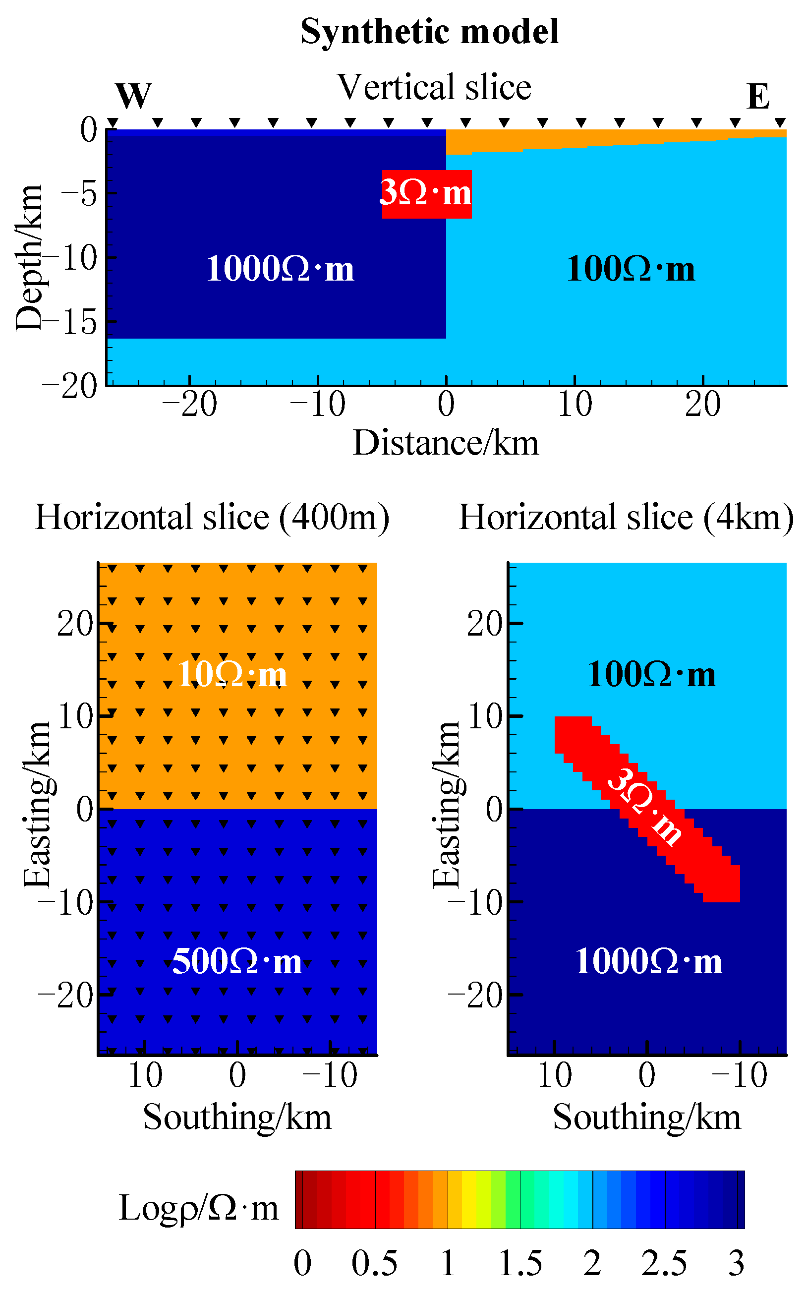
3.1. Synthetic Model

For the synthetic tests, we used some variants on an Oblique Conductor Model, which was based on the model from Ledo [46], as illustrated in Figure 1. The model comprises a regional 2-D resistivity structure formed by two half-layers of 1000 Ω·m (west side) and 100 Ω·m (east side) with their bottom at 15.75 km depth. The western half layer was covered by a horizontal layer of 500 Ω·m with its bottom at 0.5 km depth, while the eastern half layer was covered by an inclined layer of 10 Ω·m with a dip angle of approximately 3°. In the central domain, a conductive block (3 Ω·m) of approximately 20 × 4 × 4 km3 was embedded in the regional 2-D structure with its top at 3 km deep. The major axis of the conductive block obliquely crossed (45°) the contact plane of the two half layers. The bottom of the model (below the depth of 15.75 km) was set as a half space of 100 Ω·m.
The forward responses of the synthetic model were calculated for an 18 × 10 station array with a 3 km station distance that covered the model subsurface structure using the ModEM code [15,16]. The 23 periods used were evenly spaced on the logarithmic scale in a range of 0.003 and 1000 s. The central domain of the grid comprised 50 × 30 × 51 cells with a horizontal discretization of 1 km × 1 km, which was padded by five planes from the edges of the central domain outward to the boundaries with the cells lateral size increasing by a factor of two. The thickness of the top layer was 100 m, and the thicknesses of the subsequent layers increased by a factor of 1.2 in the z direction. The large 3-D grid then consisted of 60 × 40 × 51 cells in the east–west, north–south, and vertical directions, respectively.

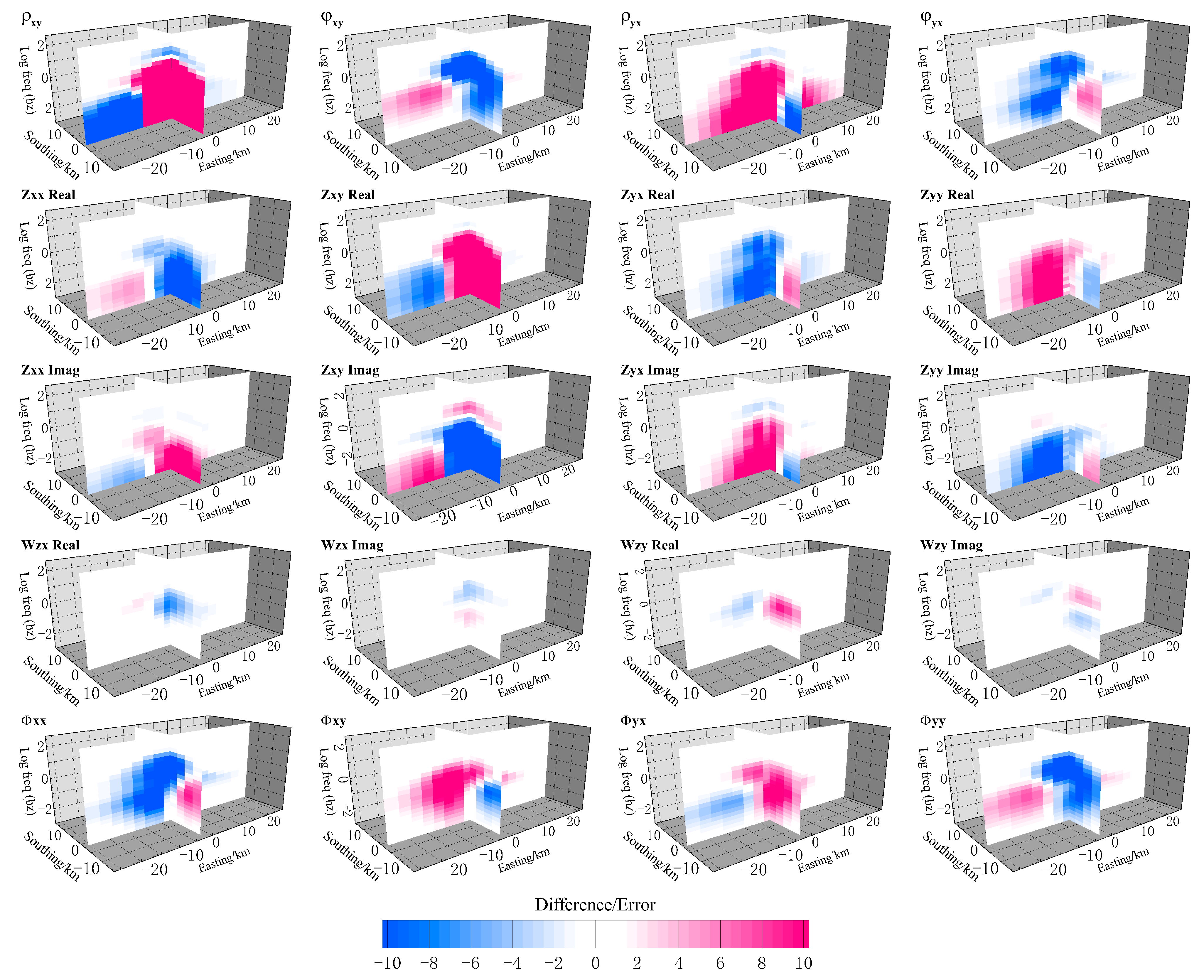
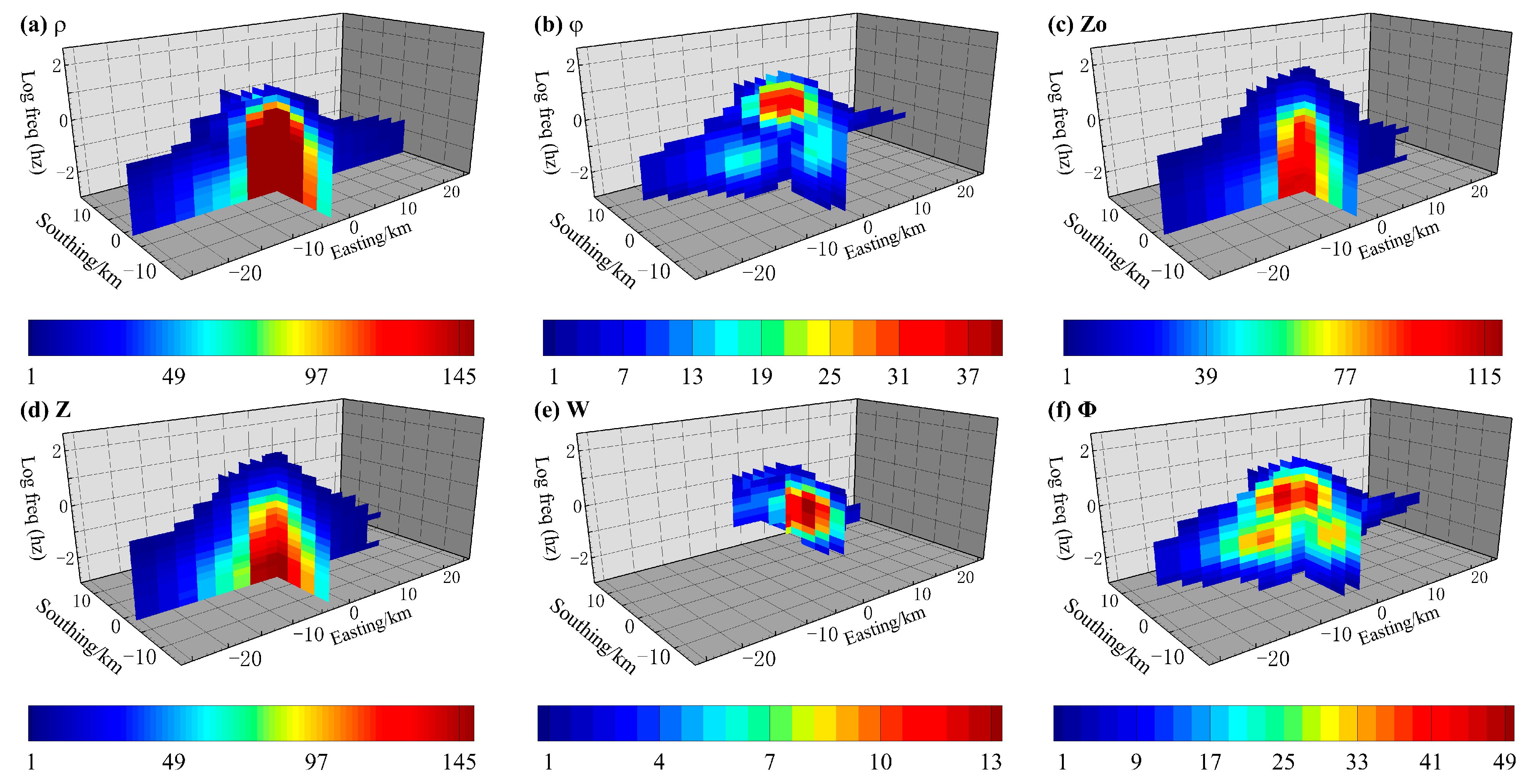
3.2. Sensitivity Analysis

The examination scheme started with a nonlinear sensitivity test, which was performed to identify the spatial responsiveness of the oblique conductor and to characterize and quantify the effects of this conductor on the MT and MV transfer functions. The nonlinear sensitivity test involved two steps: (1) we calculated the forward responses of the background regional 2-D resistivity structure without anomaly and that of the regional 2-D resistivity structure with the embedded oblique conductor; (2) the resulting forward responses were used to calculate the differences and sensitivity values for each period and station following a formula introduced by Campanyà et al. [33].
To highlight the sensitivity of the data responses to the anomaly concerning the presence of the data errors, the differences between the forward responses were divided by the assumed error. We defined the errors for the impedance tensor data relative to the amplitude of the Z elements; namely, error levels of 0.03 × |Zxy× Zyx|1/2 were adopted for all the impedance components. For the dimensionless tipper vector W responses, we adopted constant error bounds of 0.03. Although the phase tensor is a dimensionless quantity too, the error levels of the phase tensor responses here were set at 0.05 × |Φxx× Φyy|1/2 for all Φ components instead of a constant error because the relation of the amplitude of a phase tensor element to the changes in the subsurface resistivity is highly nonlinear [37].
The contoured pseudosections of the effects of the conductive block are shown in Figure 2. Each subdiagram contains two perpendicular contoured pseudosections, the distance along the east–west profile (y = 0) on the abscissa, the distance along the south–north profile (x = 0) on the ordinate, and the period (on a decadic logarithm scale) along the vertical coordinate. The white zones denote the difference values (between −1 and 1) within the assumed errors, showing the periods for the various components at the sites that are insensitive to the anomaly. The blue and red zones represent the periods at highly sensitive sites, where the responses to the anomaly were several standard deviations outside of the assumed errors. From the calculated differences for each period and station, it can be seen that the effect of the anomalous block at a given site and period was determined by the transfer function types that were employed. Specifically, the ρ responses were similar to the Z responses, the anomaly affected a long range of periods for these two responses, and the effect continued to the longest period. For the different components of the impedance tensor Z, the period range affected by the same anomaly for on-diagonal components was narrower than that for the off-diagonal components Zo. In addition, the φ responses (impedance phase) were similar to the Φ responses; this is because the phase tensor Φ is a function of the impedance and can be written as a diagonal matrix with its components equal to the tangents of the conventional impedance phases in the layered 1-D structure [10]. Meanwhile, all of these MT responses were more sensitive at the sites above the anomaly. However, the W responses were more sensitive at the sites located at the edge of the anomaly due to the absence of a vertical field above the laterally uniform earth, where the greatest effects in the W were off to the anomaly edge [47]. Furthermore, the same anomaly affected a narrower range of periods for the Φ and W responses than that for the Z responses. The reasoning behind this is that the galvanic charges imposed on the boundaries of the conductivity contrasts generate magnetic effects and electric effects simultaneously; among them, the magnetic effects of the charges fall off rapidly with the increasing period, while the local nature of the electric fields is strong distortion from the charges on the boundaries, and the electric effects are frequency-independent and persist for longer periods in the inductive case [48]. It is worth noting that the high difference values reflected in the different data responses were mostly distributed on the west side, where there were enormous electrical differences between the embedded anomaly body and the background.
The accomplished quantification for the effect of the anomaly on the different responses illustrated in Figure 3, which comprises six subdiagrams of pseudosections, represented the sensitivity of the different transfer functions’ data, respectively. The sensitivity values of the ρ and Z responses were close, which were the highest among all the data responses, the sensitivity values of the off-diagonal impedance Zo were slightly lower than those, and the sensitivity values of the φ and W responses were approximately equal to half of the Zo responses, while the lowest sensitivity values obtained by the W responses. The increased sensitivity values of the Z responses relative to the Zo responses suggest that the use of the on-diagonal components of Z introduces the complementary information that enhances the resolution. The low sensitivity values obtained by the Φ and W responses indicate the insufficiency of the information about the absolute values of the subsurface resistivity in these dimensionless physical quantities. However, both of these are primarily sensitive to the variations of resistivity structure, which can be inferred from the distribution of those sites and periods associated with the Φ and W responses sensitive to the anomaly.
As another illustration of the sensitivity analysis, we also considered the sensitivity functions, namely the Jacobian. Six sites in an oblique line crossing the buried conductor were used to implement the sensitivity function calculations of different data responses. The used periods were set up to 1 s, 10 s, and 100 s. The results of these calculations are illustrated in Figure 4, which give the data perturbation resulting from a model resistivity perturbation. The gradients of the Zo and Z responses were the highest among all the data responses, and the gradient of the ρ + φ responses had moderate values; the gradients of the W and Φ responses, however, were three orders of magnitude lower than that of the Z responses. The calculation results suggest that the same model resistivity perturbation could result in distinct perturbations for different data responses. The low perturbations obtained by the W and Φ responses indicate the deficiency of the sensitivity to the model resistivity variations, while the medium–high perturbations obtained by the ρ + φ, Zo, and Z responses indicate sufficient sensitivity to the model resistivity variations. Although the sensitivity magnitude of the Zo was similar to that of the Z, the range of perturbations for the Z responses was a little bit larger than that for the Zo responses. This effect of the sensitivity enhancement was consistent with that of the sensitivity quantification test mentioned above (as shown in Figure 3).

3.3. Three-Dimensional Inversion Tests

For the subsequent numerical experiment, we performed a 3-D inversion of different transfer functions’ data utilizing a quasi-Newton method based on the L-BFGS formula, which was achieved by a modification to the ModEM code [16]. The solution mesh was chosen in common with the forward mesh described above, which comprised 60 × 40 × 51 cells beneath the station array. Five inversions were performed to examine and evaluate the capability of different transfer functions’ data to characterize the subsurface by themselves, that is, the inversions of the ρ + φ, Zo, Z, W, and Φ responses individually. Three additional inversions were performed to appraise the advantages and disadvantages of complementing the Zo, Z, and Φ responses with the W responses. Hence, the final inversions were (1) ρ + φ, (2) Zo, (3) Z, (4) W, (5) Φ, (6) Zo + W, (7) Z + W, and (8) Φ + W. For the subsequent inversions, all these used responses were perturbed by the same scheme described in the sensitivity analysis. The heavily penalized deviations from a prior model can lead to erroneous and misleading 3-D inversion results, particularly in environments with strong conductivity contrasts; hence, the prior model setting is important in retrieving the subsurface [28,37]. Thus, we executed a test to choose the prior model by inverting different transfer function data with four homogeneous half-space models of 10, 100, 300, and 1000 Ω·m, respectively. The results of the test are displayed in Figure S1, where the inversion results using a prior model of 100 Ω·m obtained the recovery of the electrical resistivity values most similar to the synthetic model. Based on this test, the chosen prior model for all the presented inversions was set as a homogeneous half space of 100 Ω·m. In addition, a cooling method for the damping factor was adopted to improve the stability of the inversion, and the initial damping factor value was set to 10. In addition, we inverted the Z and W responses with different model covariance smoothing parameters of 0.1, 0.2, 0.3, 0.4, 0.5, and 0.7 to discuss the influence of the model covariance matrix on the inversion results, as the model norm’s behavior is controlled by the model covariance matrix. The results of this test are displayed in Figure S2, where a model covariance smoothing parameter of 0.3 yielded the most effective inversion result. Therefore, the model covariance smoothing parameter for all the presented inversions was uniformly set to 0.3, with two smoothing passes in each direction.
The corresponding final inversion models were obtained when the acceptable overall normalized root mean square (nRMS) misfit was achieved. The fit of the data of each inversion process is shown in Figure 5; that is, the summed nRMS was calculated at each station and provided valuable information on how the data misfit was distributed across the array. It can be seen that the misfits were distributed smoothly through the array for different transfer functions’ type. Even though some larger nRMS associated with the inversion results of the ρ + φ responses were observed, the particular transfer functions’ type or station locations had no overfitting problem. These overall good fits denote that all the inversion results have a lower average variance between the original synthetic model and the final inversion model. Table 1 shows how the objective function value changes during the iteration for each type of inversion. It can be seen that all the inversions can converge to a similar level of the objective function value, which suggests the inversions have worked properly. However, for the inversion of the W, Φ, and Φ + W responses, the decreases in the objective function values were not significant. In addition, the use of the W responses as complements to the Zo responses significantly accelerated the convergence of the inversion (i.e., reduced the maximum number of iterations from 130 to 87). However, this situation was completely opposite in the joint inversion of the two types of dimensionless quantity (i.e., the Φ + W responses).

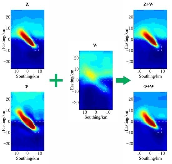
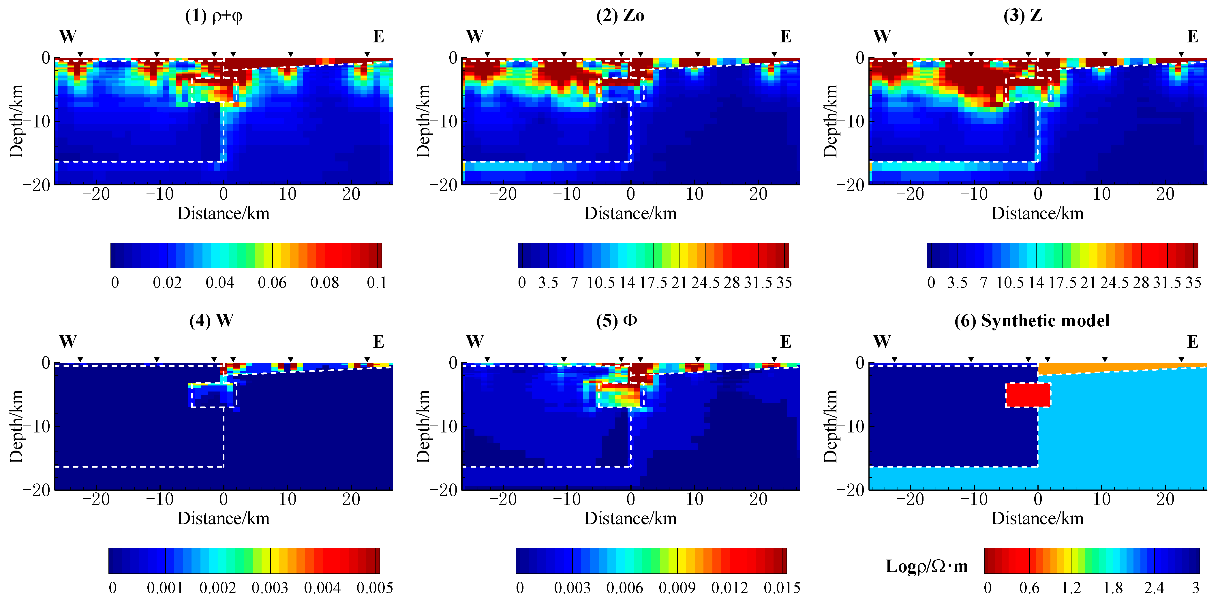
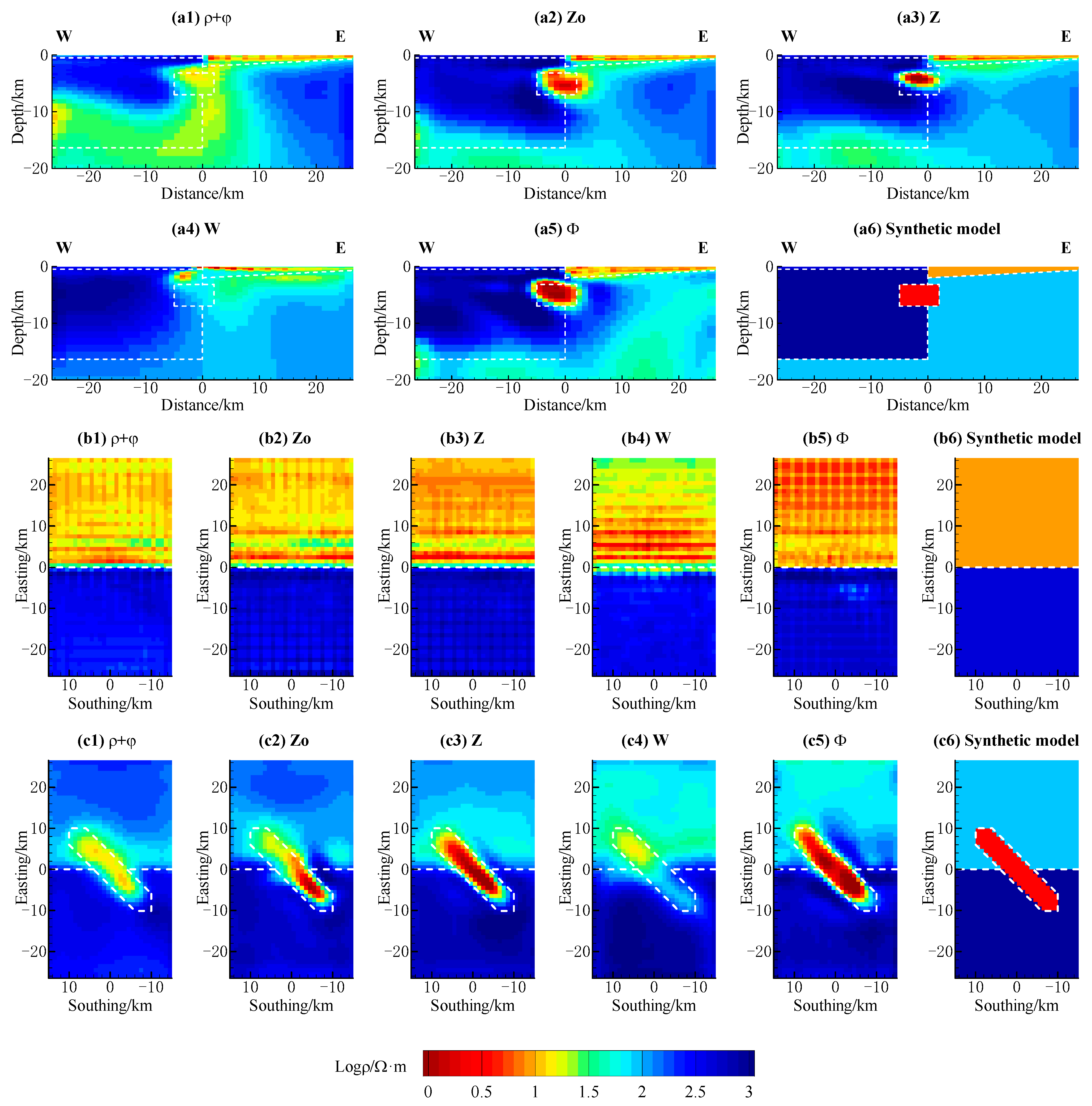
3.3.1. Results of Inverting the MT and MV Transfer Functions Individually

The models resulting from the inversion of the MT and MV transfer functions data individually are displayed in Figure 6, where Figure 6a1–a6 illustrates the electrical resistivity model beneath a W–E profile (y = −1.5 km), and the following Figure 6b1–b6,c1–c6 represents the horizontal slices at 400 m deep and 4000 m deep, respectively. The corresponding final inversion models of all the responses characterized the main structures and resistivity contrasts of the synthetic model in approximately the correct location. The inversion results of the Zo, Z, and Φ responses recovered the closest resistivity value to the true value of the 3 Ω·m for the oblique conductive block and well constrained the lateral extent of the oblique conductive block, although the absolute resistivity of the eastern conductive block was overestimated when inverting the Zo responses. Although the inversion results of the Zo responses depicted the boundaries of the oblique conductive block in the background of high resistivity (1000 Ω·m), the boundary characterization of the oblique conductive block in the background of low resistivity (100 Ω·m) was distorted. Additionally, the inversion results of the Φ responses better defined the upper and lower boundary of the conductive block in the background of low resistivity (100 Ω·m, which was the same as that in the prior model), whereas the lower boundary of the recovered conductive block appeared at a shallower depth than in the real model when the Z responses were used in the inversion. Note that the inversion results of the Φ responses defined a wrong upper boundary in the background of high resistivity (1000 Ω·m); the reasoning behind this could be related to the initial resistivity of the prior model.
In contrast, the corresponding final inversion models of the ρ + φ and W responses could only infer the lateral extent of the oblique conductive block; although the magnitude of the resistivity contrast between the two half layers (including that between the two covers) was reproduced correctly. When only inverting the W responses, the inversion model was unable to define the continuity of the oblique conductive block; the resulting conductive block was characterized as two halves (high resistivity in the western part and low resistivity in the eastern part). This is because the W responses lacked information about the absolute resistivity values but contained information about the variations in the relative conductivity in the subsurface. There was a serious distortion in the characterization of the vertical boundary of the conductive block when inverting the ρ + φ responses, which manifested as redundant anomalies below the oblique conductive block. The reasoning behind the poorer recovery of the resistivity values and geometry of the oblique conductive block with the ρ + φ responses inversion is that the imaginary part of the Jacobi matrix was ignored when processing the apparent resistivity and impedance phase data in this paper; therefore, the accuracy of the inversion decreased. The outcome of our study indicated that the recovery of the subsurface resistivity structure showed a strong dependence on the type of transfer functions.

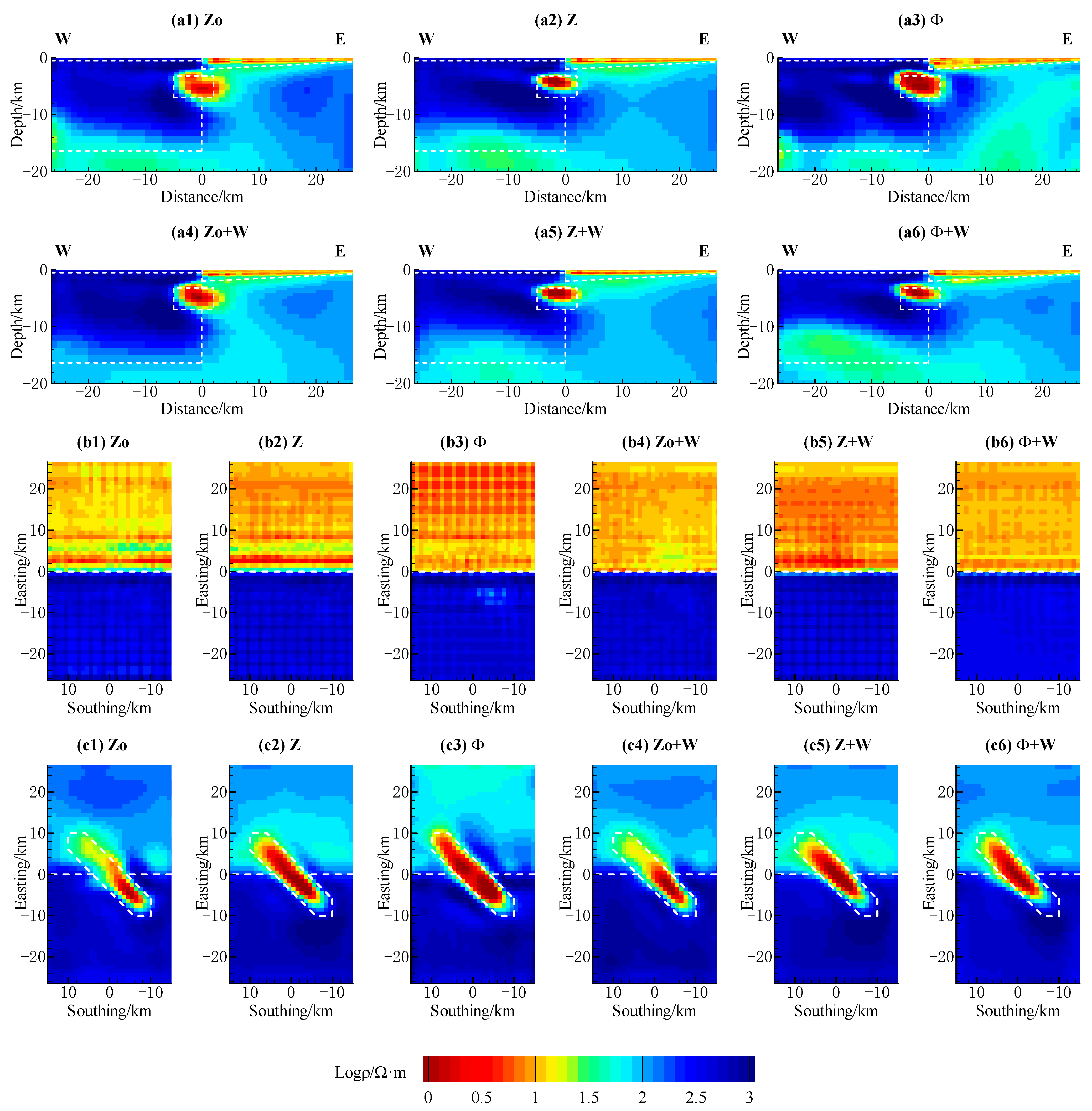
3.3.2. Results of Inverting the MT and MV Transfer Functions Jointly

The joint inversion results of the MT and MV transfer functions data are displayed in Figure 7 and are compared with the results of inverting the MT transfer functions data individually. It can be seen that all the joint inversion results reproduced a more accurate magnitude of the resistivity contrast between the two half layers. The use of the W responses as complements to the Zo and Z responses in the inversion slightly improved the resolution of the oblique conductive block. In these cases, the recovery of the resistivity values and geometry of the oblique conductive block was significantly improved. Particularly for complementing the Zo responses with the W responses, a more homogeneous resistivity distribution of the oblique conductive block was defined. However, the lower boundary of the oblique conductive block seemed to appear at a shallower depth when complementing the Φ responses with the W responses. These results indicate that the W responses were insufficient to characterize the variations of conductivity in the vertical direction, but the corresponding final inversion models preferably constrained the lateral variations of the conductivity when inverting the W responses as a complement to the Zo, Z, and Φ responses.

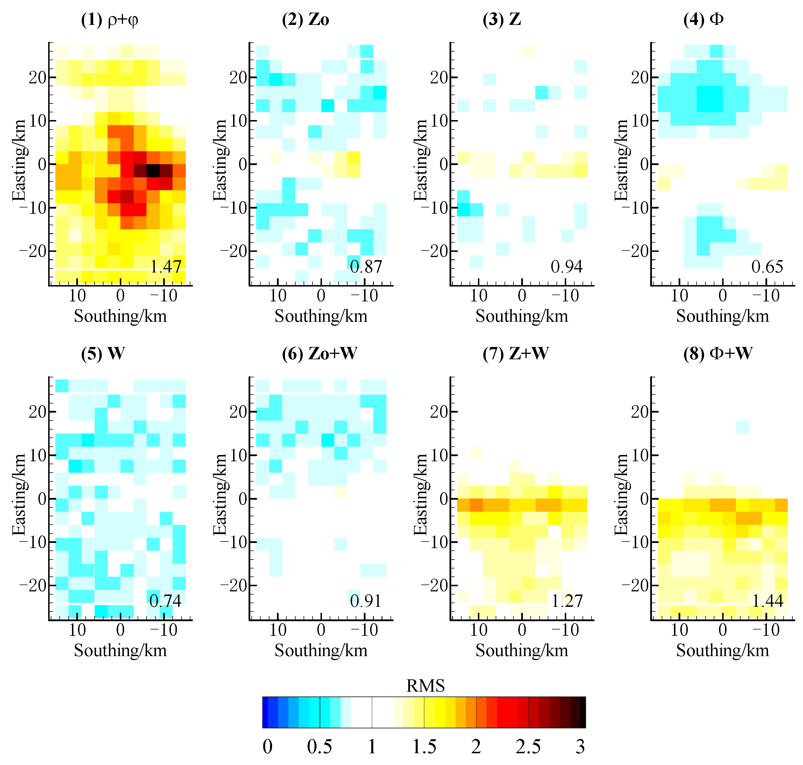
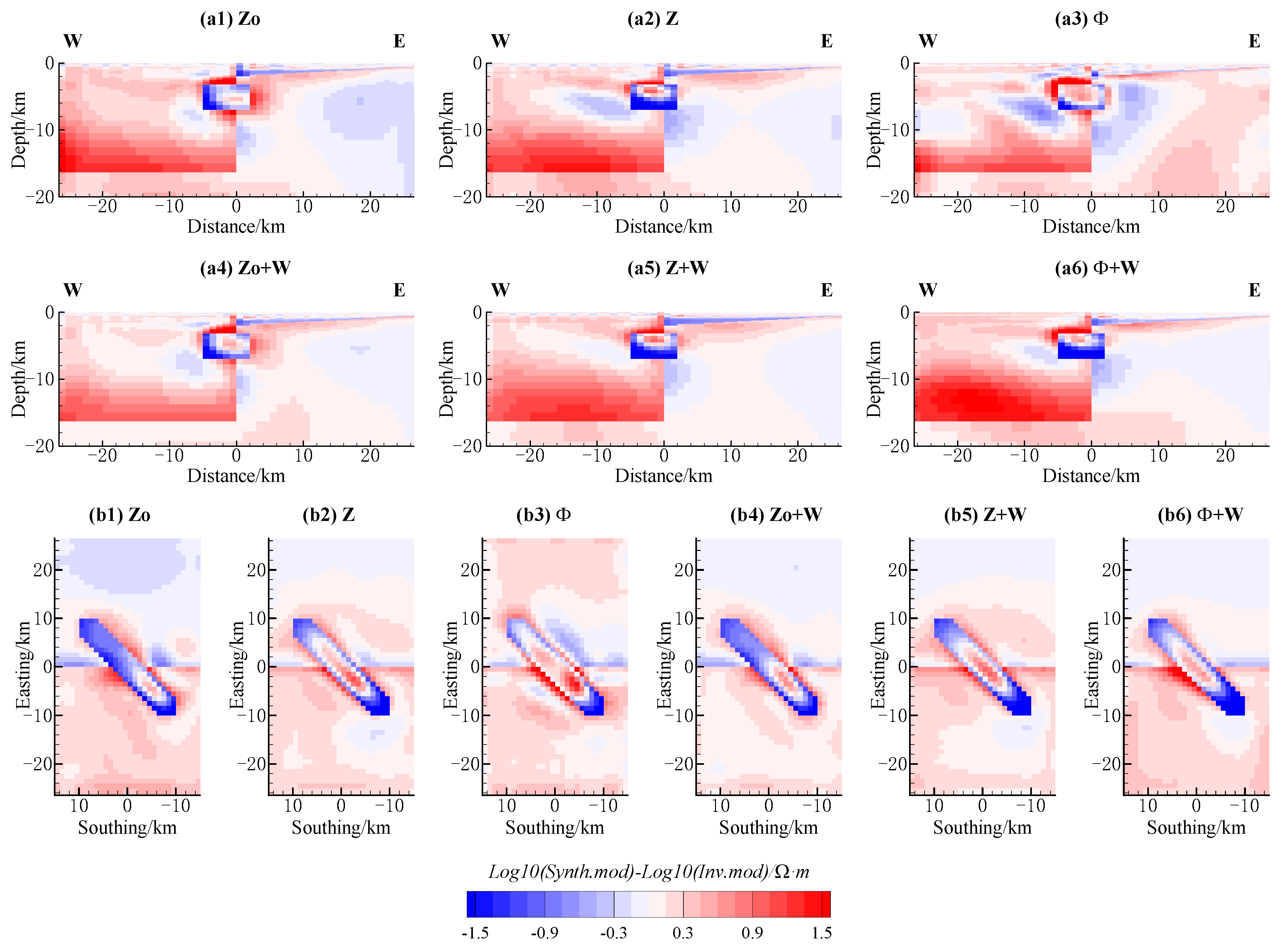
3.3.3. Assessment of the Model’s Accuracy

In order to quantify how well the models obtained from the inversion process reproduced the synthetic model, we calculated the differences between them in model space. The results with a focus on the vertical structures below the W–E profile and the lateral structures at a depth of 4000 m are shown in Figure 8. The differences between the synthetic model and the inversion models were calculated using the decadic logarithm electrical resistivity values. The colors indicate the resistivity biases between the inversion model and the synthetic model, where the red and blue colors, respectively, indicate the results that were more conductive and more resistive than the synthetic model, respectively, and the white color indicates an almost-perfect fit between the final inversion model and the original synthetic model. The average differences for each type of inversion are shown in Table 2. It can be seen that all the inversion models better defined the geometry of the conductive block, although the electrical resistivity values of the conductive block edges were more resistive than in the synthetic model. The results from the inversion processes complementing the W responses with the Zo, Z, and Φ responses significantly improved the recovery of the electrical resistivity values of the regional 2-D resistivity background, showing a more homogeneous resistivity distribution and correctly reproducing the magnitude of the resistivity contrast between the two half layers. However, the electrical resistivity values associated with the lower boundary of the conductive block were more resistive than in the synthetic model when the W responses were involved in the inversion of the Φ responses.

4. Discussion

In this work, we performed sensitivity tests on the different MT and MV transfer functions, including the ρ, φ, Zo, Z, W, and Φ responses. The results of our numerical experiment suggest that the difference in the sensitivity of the Z and Zo responses to the anomalies directly leads to the difference in their capabilities to recover the subsurface electrical resistivity. The capacity for recovering the detail of the geoelectrical structures (Figure 6) was remarkably improved when the on-diagonal components of Z were used. Although the sensitivity of the ρ responses was similar to that of the Z responses, the ρ + φ responses were not good types of data to define the boundaries of the subsurface geoelectrical structure and even resulted in redundant artifacts under the oblique conductive block (Figure 6), which may be caused by ignoring the imaginary part of the Jacobi matrix. Inspecting the sensitivities obtained from the W responses, the sensitivity associated with the oblique conductive block was the lowest, and the locations and periods responsive to the anomaly body appeared as a narrow zone. This property of the W responses hence resulted in the worst recovery ability of the subsurface geoelectrical structure. For the Φ responses, the sensitivity in connection with the anomaly body was moderate, and the locations and periods responsive to the anomaly body were sensitive at the edges of the structures, making the Φ responses a good type of data to define the boundaries of the structures. The consequences of this property in the inversion process can be seen in Figure 6, Figure 7 and Figure 8, where the models obtained by inverting the Φ responses were closer to the original synthetic model; in particular, the boundary of the oblique conductive block was better than that by inverting other data types. Although the W responses were intrinsically less sensitive to the existence of the anomaly than the Zo, Z, and Φ responses, it effectively improved the ability to recover the detail of the geoelectrical structures when it was complemented with the Zo or Z responses. This improvement was more remarkable for the off-diagonal components of Z, the models including the W responses obtained the horizontal boundary of the oblique conductive block closer to the original model (Figure 7), and the difference between the final inversion model and the original synthetic model was smaller than that obtained by inverting the Zo responses individually (Figure 8 and Table 2). However, the use of the W responses as an accompaniment to the commonly used Φ responses obtained the incorrect bottom boundaries of the geoelectrical structures, which increased the difference between the final inversion model and the original synthetic model (Figure 8 and Table 2), even though the recovery of the background resistivity was better.
Many previous studies have emphasized that the use of diagonal elements in the inversion of the full impedance tensor Z possesses a superior capacity to reproduce the dimensionality of the 3-D geoelectrical structures [28,29]. These conclusions can be validated by the results from the inversion of the Z and Zo responses in our work; it can be seen that the use of the Z responses aided the superior determination of the conductive block than when using the Zo responses, including the characterization of the geometry and the absolute electrical resistivity values (Figure 6). The phase tensor Φ was more sensitive to the vertical contrasts and was unaffected by galvanic distortion; the approach of inverting the phase tensor Φ is highly recommended for 3-D inversion [37,39]. Although the results of inverting only the Φ responses presented a stronger dependence on the resistivity level of the prior model (Figure S1), complementing the Φ responses with the W responses can lead to the superior recovery of the absolute resistivity structure [38]; this inference is supported by the recovery of the background resistivity shown in our work (Figure 7 and Figure 8). The tipper vector W was more indicative of the lateral contrasts; thus, the results of inverting the W responses as a complement to the Zo, Z, and Φ responses provided preferable lateral contrasts of conductivity, particularly for the recovery of the background resistivity model (Figure 7 and Figure 8).

5. Conclusions

This study provided an appraisal of the MT and MV transfer functions’ selection in a 3-D inversion by utilizing a quasi-Newton method based on the L-BFGS formula. The inversion result showed that the 3-D inversion of either the Z or Φ responses presented a superior ability to recover the electrical resistivity values of the oblique conductive block as well as the background resistivity model. Moreover, the joint inversions of the Zo, Z, or Φ responses with the W responses possessed a superior imaging of the geometry and horizontal continuity of the oblique conductive block. From these results, we conclude that the ability to recover the subsurface electrical resistivity depends on the sensitivity of the transfer function. The greater the transfer function resistivity perturbation produced by the model resistivity perturbation, the stronger the ability of the transfer function to recover the underground structure. Comparing the effect of the individual and joint inversion of different transfer functions is an important way to determine the advantages of each transfer function and achieve a more reasonable interpretation.

Supplementary Materials

The following supporting information can be downloaded at: https://www.mdpi.com/article/10.3390/rs15133416/s1, Figure S1: Resistivity models obtained from inversion of different transfer functions data, displayed as horizontal slices at depth of 4 km and across the array. Horizontal slices showing the results of the inversion processes with homogeneous half-space models of (a) 10, (b) 100, (c) 300, and (d) 1000 Ω·m; Figure S2: Resistivity models obtained from inversion of Z and W responses with different model covariance smoothing parameters of 0.1, 0.2, 0.3, 0.4, 0.5, and 0.7, respectively. (a1–a6) illustrating the electrical resistivity model beneath a W–E profile (y = −1.5 km), the following Figures (b1–b6) and (c1–c6) representing the horizontal slices at 400 m depth and 4000 m depth, respectively.

Author Contributions

Conceptualization, H.Y. and J.D.; methodology, H.Y., H.C. and W.T.; formal analysis, H.Y. and X.C.; investigation, H.Y., J.D., H.C. and C.Z.; writing—original draft preparation, H.Y.; writing—review and editing, J.D., B.T. and W.T.; visualization, H.Y. and H.C.; funding acquisition, J.D., H.C. and X.C. All authors have read and agreed to the published version of the manuscript.

Funding

This paper was financially supported by the National Natural Science Foundation of China (42130811, 41864004, 42274185, 41674077) and the Science and Technology Project of Jiangxi Province (20204BCJL23058, 2022KSG01003, 20224BAB203046).

Data Availability Statement

Data associated with this research are available and can be obtained by contacting the corresponding author.

Conflicts of Interest

The authors declare no conflict of interest.

References

  1. Zhdanov, M.S. Geophysical Electromagnetic Theory and Methods; Elsevier Science: Amsterdam, The Netherlands, 2009; Volume 43. [Google Scholar]
  2. Berdichevsky, M.N.; Zhdanov, M.S. Advanced Theory of Deep Geomagnetic Sounding; Elsevier Science: Amsterdam, The Netherlands; Oxford, UK; New York, NY, USA; Tokyo, Japan, 1984. [Google Scholar]
  3. Berdichevsky, M.N.; Dmitriev, V.I. Models and Methods of Magnetotellurics; Springer: Berlin/Heidelberg, Germany, 2008. [Google Scholar]
  4. Tikhonov, A.N. On determining electrical characteristics of the deep layers of earth’s crust. Doklady 1950, 73, 295–297. [Google Scholar]
  5. Cagniard, L. Basic theory of the magneto-telluric method of geophysical prospecting. Geophysics 1953, 18, 605–635. [Google Scholar] [CrossRef]
  6. Hermance, J.F.; Thayer, R.E. The Telluric-Magnetotelluric Method. Geophysics 1975, 40, 664–668. [Google Scholar] [CrossRef]
  7. Kruglyakov, M.; Kuvshinov, A. 3-D inversion of MT impedances and inter-site tensors, individually and jointly. New lessons learnt. Earth Planets Space 2019, 71, 4. [Google Scholar] [CrossRef] [Green Version]
  8. Berdichevsky, M.N. Electrical Prospecting with the Telluric Current Method; Colorado School of Mines: Golden, CO, USA, 1965; Volume 60, pp. 1–216. [Google Scholar]
  9. Yungul, S.H. Telluric Sounding-A Magnetotelluric Method Without Magnetic Measurements. Geophysics 1966, 31, 185–191. [Google Scholar] [CrossRef]
  10. Caldwell, T.G.; Bibby, H.M.; Brown, C. The magnetotelluric phase tensor. Geophys. J. Int. 2004, 158, 457–469. [Google Scholar] [CrossRef] [Green Version]
  11. Araya Vargas, J.; Ritter, O. Source effects in mid-latitude geomagnetic transfer functions. Geophys. J. Int. 2016, 204, 606–630. [Google Scholar] [CrossRef]
  12. Morschhauser, A.; Grayver, A.; Kuvshinov, A.; Samrock, F.; Matzka, J. Tippers at island geomagnetic observatories constrain electrical conductivity of oceanic lithosphere and upper mantle. Earth Planets Space 2019, 71, 17. [Google Scholar] [CrossRef] [Green Version]
  13. Jupp, D.L.B. Estimation of the magnetotelluric impedance functions. Phys. Earth Planet. Inter. 1978, 17, 75–82. [Google Scholar] [CrossRef]
  14. Parker, R.L. The magnetotelluric inverse problem. Geophys. Surv. 1983, 6, 5–25. [Google Scholar] [CrossRef]
  15. Egbert, G.D.; Kelbert, A. Computational recipes for electromagnetic inverse problems. Geophys. J. Int. 2012, 189, 251–267. [Google Scholar] [CrossRef] [Green Version]
  16. Kelbert, A.; Meqbel, N.; Egbert, G.D.; Tandon, K. ModEM: A modular system for inversion of electromagnetic geophysical data. Comput. Geosci. 2014, 66, 40–53. [Google Scholar] [CrossRef]
  17. Grayver, A.V. Parallel three-dimensional magnetotelluric inversion using adaptive finite-element method. Part I: Theory and synthetic study. Geophys. J. Int. 2015, 202, 584–603. [Google Scholar] [CrossRef] [Green Version]
  18. Kordy, M.; Wannamaker, P.; Maris, V.; Cherkaev, E.; Hill, G. 3-dimensional magnetotelluric inversion including topography using deformed hexahedral edge finite elements and direct solvers parallelized on symmetric multiprocessor computers–Part II: Direct data-space inverse solution. Geophys. J. Int. 2016, 204, 94–110. [Google Scholar] [CrossRef] [Green Version]
  19. Conway, D.; Alexander, B.; King, M.; Heinson, G.; Kee, Y. Inverting magnetotelluric responses in a three-dimensional earth using fast forward approximations based on artificial neural networks. Comput. Geosci. 2019, 127, 44–52. [Google Scholar] [CrossRef]
  20. Daubechies, I. Ten Lectures on Wavelets; Society for Industrial and Applied Mathematics: Philadelphia, PA, USA, 1992; Volume 61. [Google Scholar]
  21. Torrence, C.; Compo, G.P. A Practical Guide to Wavelet Analysis. Bull. Am. Meteorol. Soc. 1998, 79, 61–78. [Google Scholar] [CrossRef]
  22. Pucciarelli, G. Wavelet Analysis in Volcanology: The Case of Phlegrean Fields. J. Environ. Sci. Eng. A 2017, 6, 300–307. [Google Scholar] [CrossRef] [Green Version]
  23. Nittinger, C.G.; Becken, M. Inversion of magnetotelluric data in a sparse model domain. Geophys. J. Int. 2016, 206, 1398–1409. [Google Scholar] [CrossRef] [Green Version]
  24. Liu, Y.; Farquharson, C.G.; Yin, C.; Baranwal, V.C. Wavelet-based 3-D inversion for frequency-domain airborne EM data. Geophys. J. Int. 2017, 213, 1–15. [Google Scholar] [CrossRef]
  25. Miensopust, M.P. Application of 3-D Electromagnetic Inversion in Practice: Challenges, Pitfalls and Solution Approaches. Surv. Geophys. 2017, 38, 869–933. [Google Scholar] [CrossRef]
  26. Brasse, H.; Lezaeta, P.; Rath, V.; Schwalenberg, K.; Soyer, W.; Haak, V. The Bolivian Altiplano conductivity anomaly. J. Geophys. Res. Solid Earth 2002, 107, EPM 4-1–EPM 4-14. [Google Scholar] [CrossRef]
  27. Siripunvaraporn, W.; Egbert, G.; Lenbury, Y.; Uyeshima, M. Three-dimensional magnetotelluric inversion: Data-space method. Phys. Earth Planet. Inter. 2005, 150, 3–14. [Google Scholar] [CrossRef]
  28. Tietze, K.; Ritter, O. Three-dimensional magnetotelluric inversion in practice—The electrical conductivity structure of the San Andreas Fault in Central California. Geophys. J. Int. 2013, 195, 130–147. [Google Scholar] [CrossRef] [Green Version]
  29. Kiyan, D.; Jones, A.G.; Vozar, J. The inability of magnetotelluric off-diagonal impedance tensor elements to sense oblique conductors in three-dimensional inversion. Geophys. J. Int. 2014, 196, 1351–1364. [Google Scholar] [CrossRef] [Green Version]
  30. Sasaki, Y.; Meju, M.A. Three-dimensional joint inversion for magnetotelluric resistivity and static shift distributions in complex media. J. Geophys. Res. Solid Earth 2006, 111, 218–226. [Google Scholar] [CrossRef] [Green Version]
  31. Slezak, K.; Jozwiak, W.; Nowozynski, K.; Orynski, S.; Brasse, H. 3-D studies of MT data in the Central Polish Basin: Influence of inversion parameters, model space and transfer function selection. J. Appl. Geophys. 2019, 161, 26–36. [Google Scholar] [CrossRef]
  32. Booker, J.R. The magnetotelluric phase tensor: A critical review. Surv. Geophys. 2014, 35, 7–40. [Google Scholar] [CrossRef]
  33. Campanyà, J.; Ogaya, X.; Jones, A.G.; Rath, V.; Vozar, J.; Meqbel, N. The advantages of complementing MT profiles in 3-D environments with geomagnetic transfer function and interstation horizontal magnetic transfer function data: Results from a synthetic case study. Geophys. J. Int. 2016, 207, 1818–1836. [Google Scholar] [CrossRef] [Green Version]
  34. Siripunvaraporn, W.; Egbert, G. WSINV3DMT: Vertical magnetic field transfer function inversion and parallel implementation. Phys. Earth Planet. Inter. 2009, 173, 317–329. [Google Scholar] [CrossRef]
  35. Löwer, A.; Junge, A. Magnetotelluric Transfer Functions: Phase Tensor and Tipper Vector above a Simple Anisotropic Three-Dimensional Conductivity Anomaly and Implications for 3D Isotropic Inversion. Pure Appl. Geophys. 2017, 174, 2089–2101. [Google Scholar] [CrossRef]
  36. Bibby, H.M. Analysis of multiple-source bipole-quadripole resistivity surveys using the apparent resistivity tensor. Geophysics 1986, 51, 972–983. [Google Scholar] [CrossRef]
  37. Patro, P.K.; Uyeshima, M.; Siripunvaraporn, W. Three-dimensional inversion of magnetotelluric phase tensor data. Geophys. J. Int. 2013, 192, 58–66. [Google Scholar] [CrossRef] [Green Version]
  38. Tietze, K.; Ritter, O.; Egbert, G.D. 3-D joint inversion of the magnetotelluric phase tensor and vertical magnetic transfer functions. Geophys. J. Int. 2015, 203, 1128–1148. [Google Scholar] [CrossRef] [Green Version]
  39. Samrock, F.; Grayver, A.V.; Eysteinsson, H.; Saar, M.O. Magnetotelluric Image of Transcrustal Magmatic System Beneath the Tulu Moye Geothermal Prospect in the Ethiopian Rift. Geophys. Res. Lett. 2018, 45, 12847–12855. [Google Scholar] [CrossRef] [Green Version]
  40. Munch, F.D.; Grayver, A. Multi-scale imaging of 3-D electrical conductivity structure under the contiguous US constrains lateral variations in the upper mantle water content. Earth Planet. Sci. Lett. 2023, 602, 117939. [Google Scholar] [CrossRef]
  41. Newman, G.A.; Alumbaugh, D.L. Three-dimensional magnetotelluric inversion using non-linear conjugate gradients. Geophys. J. Int. 2000, 140, 410–424. [Google Scholar] [CrossRef] [Green Version]
  42. Sasaki, Y. Full 3-D inversion of electromagnetic data on PC. J. Appl. Geophys. 2001, 46, 45–54. [Google Scholar] [CrossRef]
  43. Newman, G.A.; Boggs, P.T. Solution accelerators for large-scale three-dimensional electromagnetic inverse problems. Inverse Probl. 2004, 20, S151–S170. [Google Scholar] [CrossRef] [Green Version]
  44. Nocedal, J.; Wright, S. Numerical Optimization; Springer Science & Business Media: Berlin/Heidelberg, Germany, 2006. [Google Scholar]
  45. Yu, H.; Deng, J.Z.; Chen, H.; Chen, X.; Wang, X.X.; Zhang, Z.Y.; Ye, Y.X.; Chen, S.N. Three-dimensional magnetotelluric inversion under topographic relief based on the limited-memory quasi-Newton algorithm (L-BFGS). Chin. J. Geophys. 2019, 62, 3175–3188. [Google Scholar]
  46. Ledo, J. 2-D Versus 3-D Magnetotelluric Data Interpretation. Surv. Geophys. 2006, 27, 111–148. [Google Scholar] [CrossRef] [Green Version]
  47. Jones, A.G. Parkinson’s pointers’ potential perfidy! Geophys. J. Int. 1986, 87, 1215–1224. [Google Scholar] [CrossRef] [Green Version]
  48. Jones, A.G. Distortion of magnetotelluric data: Its identification and removal. In The Magnetotelluric Method: Theory and Practice; Cambridge University Press: Cambridge, UK, 2012; pp. 219–302. [Google Scholar]
Figure 1. The main structural feature of the synthetic model used to generate the MT and MV data. The black triangles represent the site locations.
Remotesensing 15 03416 g001
Figure 2. Contoured pseudosections of the effects of the conductive block. The white zones denote difference values (between −1 and 1) within the assumed errors, showing the periods that are insensitive to the anomaly. The blue and red zones show periods that are highly sensitive to the anomaly.
Remotesensing 15 03416 g002
Figure 3. The results of the sensitivity test give the quantification for the effect of the anomaly on the different data responses. The color zones are periods that are sensitive to the anomaly. Note that each subdiagram has a different color scale.
Remotesensing 15 03416 g003
Figure 4. The results of different sensitivity function calculations that give the data perturbation resulting from a model resistivity perturbation. The black triangles represent the six site locations used. Note that each subdiagram has a different color scale.
Remotesensing 15 03416 g004
Figure 5. The R.M.S. misfits of the 3-D inversion distribution at each MT station for different inversions with varying transfer function types.
Remotesensing 15 03416 g005
Figure 6. The results of inverting the MT and MV transfer functions individually. (a1a6) illustrate the electrical resistivity model beneath a W–E profile (y = −1.5 km), and the following figures (b1b6,c1c6) represent the horizontal slices at 400 m deep and 4000 m deep, respectively.
Remotesensing 15 03416 g006
Figure 7. The joint inversion results of the MT and MV transfer functions data are compared with the results of inverting the MT transfer functions data individually. (a1a6) illustrate the electrical resistivity model beneath a W–E profile (y = −1.5 km), and the following figures (b1b6,c1c6) represent the horizontal slices at 400 m deep and 4000 m deep, respectively.
Remotesensing 15 03416 g007
Figure 8. The differences between the corresponding final inversion models and the synthetic model.
Remotesensing 15 03416 g008
Table 1. Objective function value (ϕ) obtained from the inversion for different transfer functions.
Data Typesρ + φZoZΦWZo + WZ + WΦ + W
ϕ initial187.07806.22407.4977.9511.42408.82275.3744.69
ϕ final2.160.770.890.430.550.831.612.08
Iterations761309375318772123
Table 2. The average differences between the final inversion models and the original synthetic model.
Data TypesZoZΦZo + WZ + WΦ + W
Difference0.1270.1390.1240.1190.1320.172
Disclaimer/Publisher’s Note: The statements, opinions and data contained in all publications are solely those of the individual author(s) and contributor(s) and not of MDPI and/or the editor(s). MDPI and/or the editor(s) disclaim responsibility for any injury to people or property resulting from any ideas, methods, instructions or products referred to in the content.

