Article

Crop Type Mapping Based on Polarization Information of Time Series Sentinel-1 Images Using Patch-Based Neural Network

College of Environmental and Resource Sciences, Zhejiang University, Hangzhou 310058, China
*
Author to whom correspondence should be addressed.
Remote Sens. 2023, 15(13), 3384; https://doi.org/10.3390/rs15133384
Submission received: 8 March 2023 / Revised: 10 June 2023 / Accepted: 27 June 2023 / Published: 3 July 2023
(This article belongs to the Special Issue Advances in Agricultural Remote Sensing and Artificial Intelligence)

Abstract

:
Large-scale crop mapping is of fundamental importance to tackle food security problems. SAR remote sensing has lately received great attention for crop type mapping due to its stability in the revisit cycle and is not hindered by cloud cover. However, most SAR image-classification studies focused on the application of backscattering characteristics with machine learning models, while few investigated the potential of the polarization decomposition and deep-learning models. This study investigated whether the radar polarization information mined by polarization decomposition, the patch strategy and the approaches for combining recurrent and convolutional neural networks (Conv2d + LSTM and ConvLSTM2d) could effectively improve the accuracy of crop type mapping. Sentinel-1 SLC and GRD products in 2020 were collected as data sources to extract VH, VV, VH/VV, VV + VH, Entropy, Anisotropy, and Alpha 7-dimensional features for classification. The results showed that the three-dimensional Convolutional Neural Network (Conv3d) was the best classifier with an accuracy and kappa up to 88.9% and 0.875, respectively, and the ConvLSTM2d and Conv2d + LSTM achieved the second and third position. Compared to backscatter coefficients, the polarization decomposition features could provide additional phase information for classification in the time dimension. The optimal patch size was 17, and the patch-based Conv3d outperformed the pixel-based Conv1d by 11.3% in accuracy and 0.128 in kappa. This study demonstrated the value of applying polarization decomposition features to deep-learning models and provided a strong technical support to efficient large-scale crop mapping.

1. Introduction

According to the Food and Agriculture Organization (FAO), a total of 650 million people worldwide faced hunger in 2019. A comprehensive understanding of food cultivation is crucial for coordinating food distribution and guaranteeing food security [1]. Crop type mapping is essential for predicting crop yields, acquiring crop phenology information and agricultural monitoring [2,3,4,5]. The traditional methods for obtaining crop information primarily rely on field surveys and farmer reports, which are both time-consuming and labor-intensive [6].
Remote sensing technology has been widely used over the last decades to break through the limitations on both spatial and temporal scales. The advantages of remote sensing technology such as large-scale and dynamic monitoring have created favorable conditions for crop type mapping. Hence, many studies have revolved around crop mapping based on remote sensing data. Recently, significant improvements in the temporal, spatial, and spectral resolutions of remote sensing data have enhanced classification accuracy [7]. Crops exhibit distinct differences in remote sensing images at various phenological stages, while other land uses remain relatively stable [8]. Improved temporal resolution can better capture short-term changes of phenological growth stages in crops, making them more separable. Consequently, some studies have explored the application of synthetic aperture radar (SAR) for crop mapping [9]. The Sentinel-1 mission is designed as a two-satellite constellation; the polar-orbiting mission provides the all-weather, day-and-night SAR imagery in the C band. Sentinel-1A was launched on 13 April 2014, followed by Sentinel-1B on 25 April 2016. Researchers can access free multiple polarization data in four sensor modes. The Sentinel-1 satellite actively sends microwaves to target areas [10], and the wavelengths of the C-band are much bigger than that of the water droplets in clouds [11], which makes it immune to climatic interference. In addition, the high temporal resolution and suitable spatial resolution also make Sentinel-1 advantageous for crop mapping work.
The backscatter coefficient reflects the scattering intensity of ground objects, serving as a relatively direct SAR parameter. However, due to the random vector scattering and coherent speckle noise, a multivariate statistical description is required [12]. Polarimetric decomposition simplifies the complex scattering mechanism of ground targets into a sum of single scattering information based on complex mathematical and theoretical assumptions. This method, when applied to crop type mapping, can extract more in-depth SAR information, providing a comprehensive representation of the target’s geometric and physical properties. Common polarimetric decomposition methods include H/α decomposition, Freeman decomposition, and Huynen decomposition [12,13,14,15]. Among these, the H/α decomposition method, proposed by Cloude et al., relies on an eigenvalue analysis of the coherency matrix and is not typically used for crop type mapping tasks [13].
In classifier selection for crop type mapping, previous studies can be categorized into two approaches: (1) threshold-based classification, mainly applied to single-polarization or dual-polarization SAR data [16,17,18]; (2) machine-learning-based classification, including algorithms such as Random Forest (RF), Support Vector Machine (SVM), and Time-Weighted Dynamic Time Warping (DTW) [1,19,20]. Random Forest, an ensemble classifier, is built on decision trees generated using randomly selected samples and features, and is based on a bagging algorithm. Owing to its numerous benefits, such as reduced over-fitting, high accuracy, ability to process high-dimensional data with multiple features, and robustness against noise, RF has been regarded as a reliable classification method for crop type mapping [11].
The rapid development of computer vision and deep learning has paved the way for innovative approaches to remote sensing image analysis. In contrast to traditional machine learning, deep-learning models possess the ability to automatically extract feature information while being less affected by redundant information, thereby streamlining the research process [21,22]. Therefore, various studies have introduced recurrent neural network (RNN), one-dimensional convolutional neural networks (Conv1d), three-dimensional convolutional neural networks (Conv3d) and hybrid models combining convolutional and recurrent neural networks (Conv2d + LSTM, ConvLSTM2d) to effectively harness the spatial and temporal dimension features [23,24,25,26,27,28].
Most of the existing methods to classify the medium-resolution remote sensing images are pixel-based, neglecting spatial information from neighboring pixels [29]. A patch-based method tailored for medium-resolution remote sensing images was proposed and initially applied to land cover classification using Landsat images. The patch-based CNN demonstrated a 24% improvement in overall classification accuracy compared to pixel-based CNNs [27]. Additionally, other studies have indicated that patch-based methods provide more stable and efficient performance across various datasets, regions and land cover categories in comparison to pixel-based approaches [30].
From the perspective of classification models and inputs, most crop mapping research based on SAR images either used traditional machine learning methods as classifiers based on polarization decomposition work, or directly input traditional SAR indices or polarization features into deep-learning classifiers. Therefore, this study focuses on the effective combination of target decomposition and deep-learning methods, and aims to build a simple and efficient crop mapping classification model.
In particular, we focus on addressing the following research questions: (1) Is the performance of polarimetric decomposition features from dual-polarization SAR data sufficiently competitive when compared to the commonly used backscatter coefficient? (2) How efficiently do CNN, RNN, and their combination perform in this context? (3) Can patch-based methods effectively improve accuracy compared to pixel-based methods? The technical roadmap is shown in Figure 1.

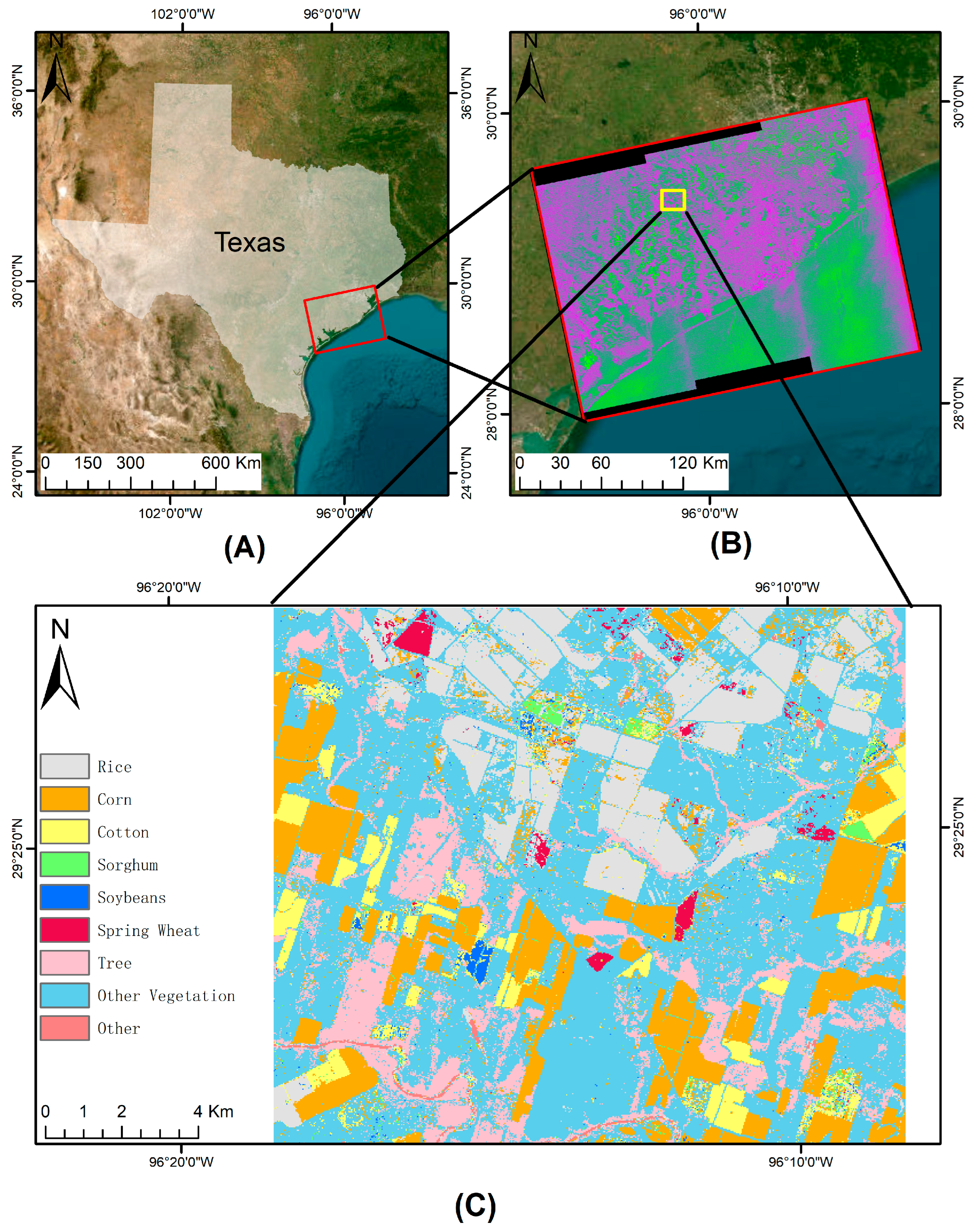
2. Study Area and Materials

2.1. Study Area

Texas, situated in the south-central region of the United States of America, spans an area of 695,662 square kilometers (268,596 square miles). The state experiences a wide range of precipitation levels, with parts of southeast Texas receiving up to 1600 mm annually. Snowfall occurs every few years in Central and East Texas. The study area in focus is located in Wharton County, which is part of the West Gulf Coastal Plain region in South Texas. This area measures approximately 16.8 km in length and 14.3 km in width, covering a total of 241.4 square kilometers. Figure 2 shows the precise location of the study area and the spatial distribution of the primary crop types. Information on the United States crop calendar can be found on the USDA website (https://ipad.fas.usda.gov/rssiws/al/crop_calendar/us.aspx (accessed on 8 March 2023)), as depicted in Figure 3.

2.2. Sentinel-1

Sentinel-1A images were acquired from Copernicus Open Access Hub (https://scihub.copernicus.eu/dhus/#/home (accessed on 30 September 2021)) for the period between 1 January 2020 and 31 December 2020. The study area was covered by a single Sentinel-1 IW mode image tile with a 10 m spatial resolution. Dual-polarization VV + VH was chosen due to its strong interaction with agricultural fields. To avoid absorption caused by morning dew on crops, an ascending orbit was employed [11,31].
This study utilized Ground Range Detected (GRD) and Single Look Complex (SLC) level-1 products, comprising 30 scenes each. Through the preprocessing of GRD products, we can obtain VV and VH band information and further calculate the values of VH/VV and VV + VH. The SLC data contains phase and amplitude information [1], facilitating polarimetric decomposition to derive Cloude decomposition features.

2.3. Cropland Data Layer
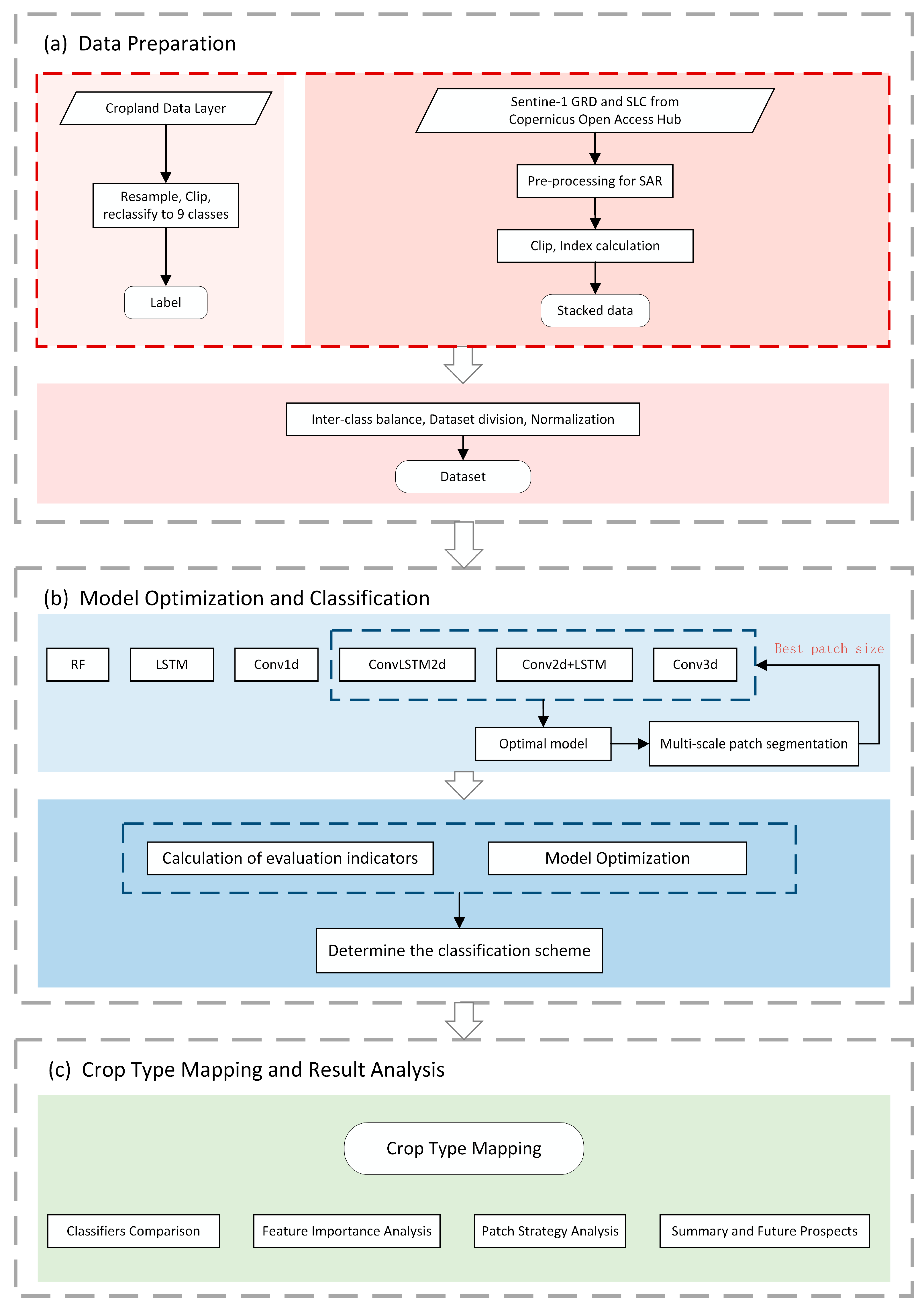
The national Cropland Data Layer (CDL) served as reference data for generating training, validation and test datasets in this study. Derived from Landsat imagery and field surveys, CDL offers over 200 crop types with a spatial resolution of 30 m [32]. Many researchers have utilized the CDL data because of its high accuracy [33]. With an overall accuracy of up to 90%, CDL data for corn and soybeans exceeds 95% accuracy [7,20]. For this study, we acquired 2020 CDL data and reclassified the object categories in the study area into nine classes, focusing on rice, corn, cotton, sorghum, soybean, and spring wheat. Remaining categories were consolidated into “Trees,” “Other Vegetation,” and “Other.” This consolidation was based on the distinct differences in SAR signals between trees, structures, and water bodies compared to low vegetation. Table 1 presents the correspondence between the original and reclassified categories.

3. Methods

3.1. Data Preparation

The Sentinel-1A GRD and SLC data were preprocessed using the SNAP software following standard procedures. The common preprocessing steps for GRD data included:
(1)
Apply orbit file, to update more accurate track information;
(2)
Thermal noise removal;
(3)
Radiometric calibration, to transform digital number values to backscatter coefficient;
(4)
Multilooking (the study skipped this step as it was already applied in the GRD product and further reduction of spatial resolution was unnecessary);
(5)
Speckle filtering, to mitigate the speckle noise, a common phenomenon in coherent systems such as SAR, which arises from large and rough surfaces incompatible with the corresponding wavelength scale. In classification applications, it is essential to remove speckle noise. The refined Lee filter, an adaptive filter known for its excellent performance, was employed for this purpose;
(6)
Terrain correction, we chose SRTM as DEM data using a bilinear interpolation resampling method [11,32,34].
The preprocessing of Sentinel-1A SLC data was carried out following a similar approach to that of GRD data, which included applying orbit file, calibration, deburst, generating polarimetric matrix, multi-looking, polarimetric speckle filter, polarimetric decomposition, and terrain correction. Deburst was employed to remove the dark regions lacking information. After generating the polarimetric matrix, we obtained C11, C12_real, C12_imag, and C22 bands. On this basis, multilooking and polarimetric speckle filter were performed. Furthermore, we obtained polarimetric decomposition features of Entropy, Anisotropy, and Alpha through polarimetric decomposition. Finally, the same parameters and datasets were applied in terrain correction as GRD [35].
As for the CDL data, they were employed as a label layer following reclassification and resampling to a 10 m spatial resolution.
After the preprocessing work, a total of 7-dimensional classification features, including VH, VV, VH/VV, VV + VH, Entropy, Anisotropy, and Alpha were extracted and stacked together to form the feature space. Each feature’s values were scaled to a 0–1 range using min–max normalization.
Due to the considerable disparity in sample sizes across categories in the study area, a class imbalance issue arose, with the largest category containing roughly 95 times more samples than the smallest one. To address this, random sampling was utilized to achieve class balance. Subsequently, the dataset was randomly divided into training, validation, and test sets at a 6:2:2 ratio, and the number of samples in each category before and after sample balancing is shown in Table 2.

3.2. Classification

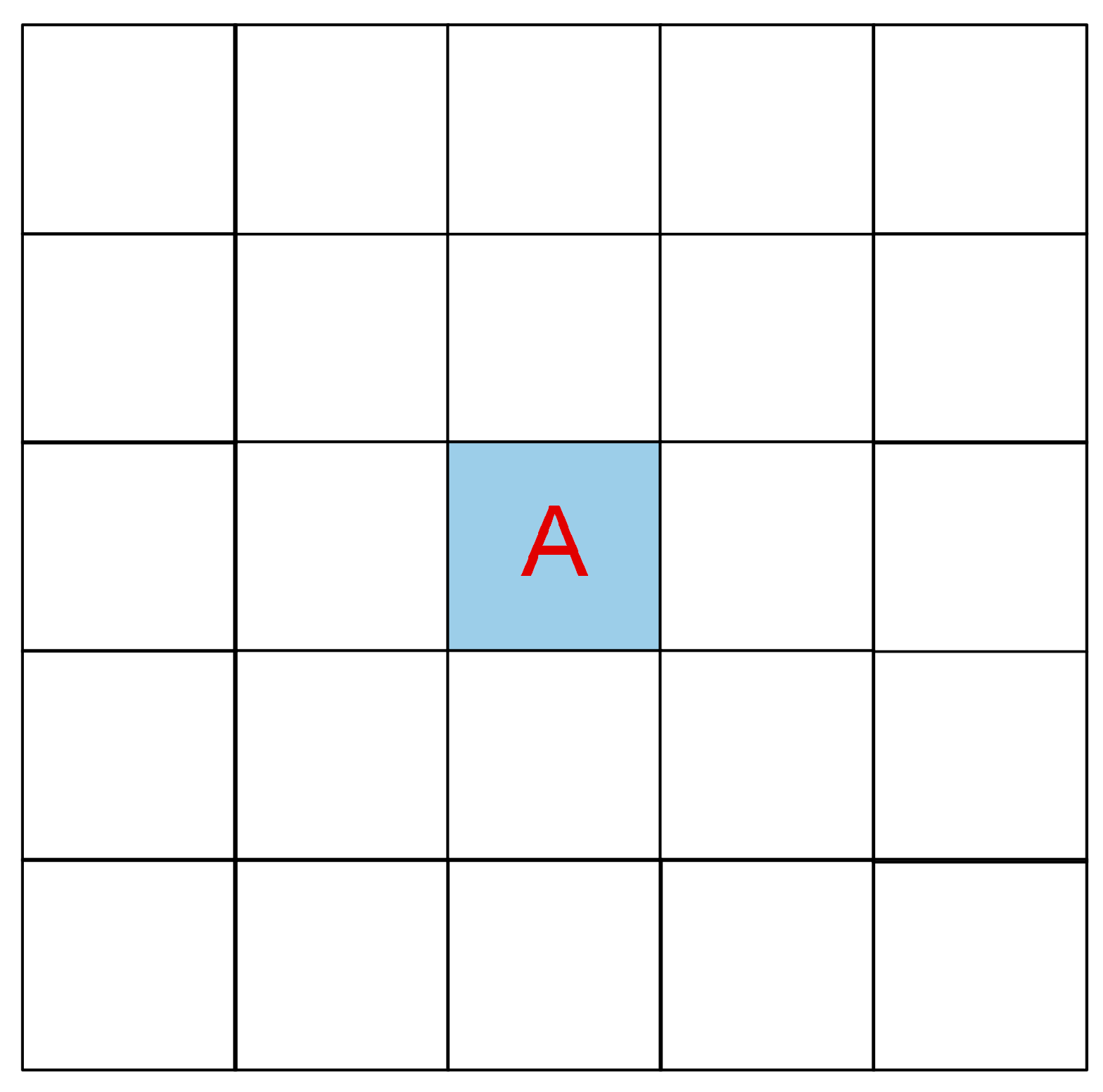
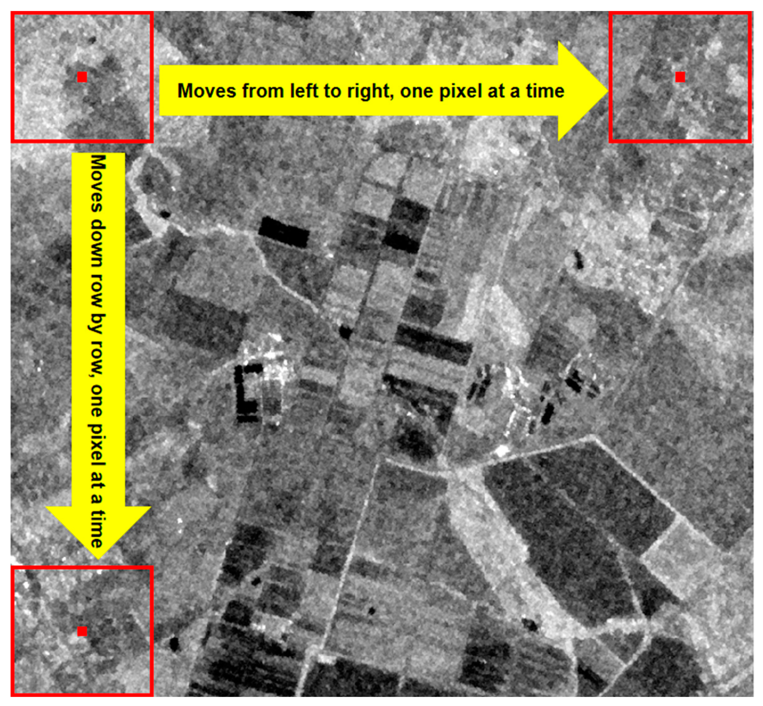
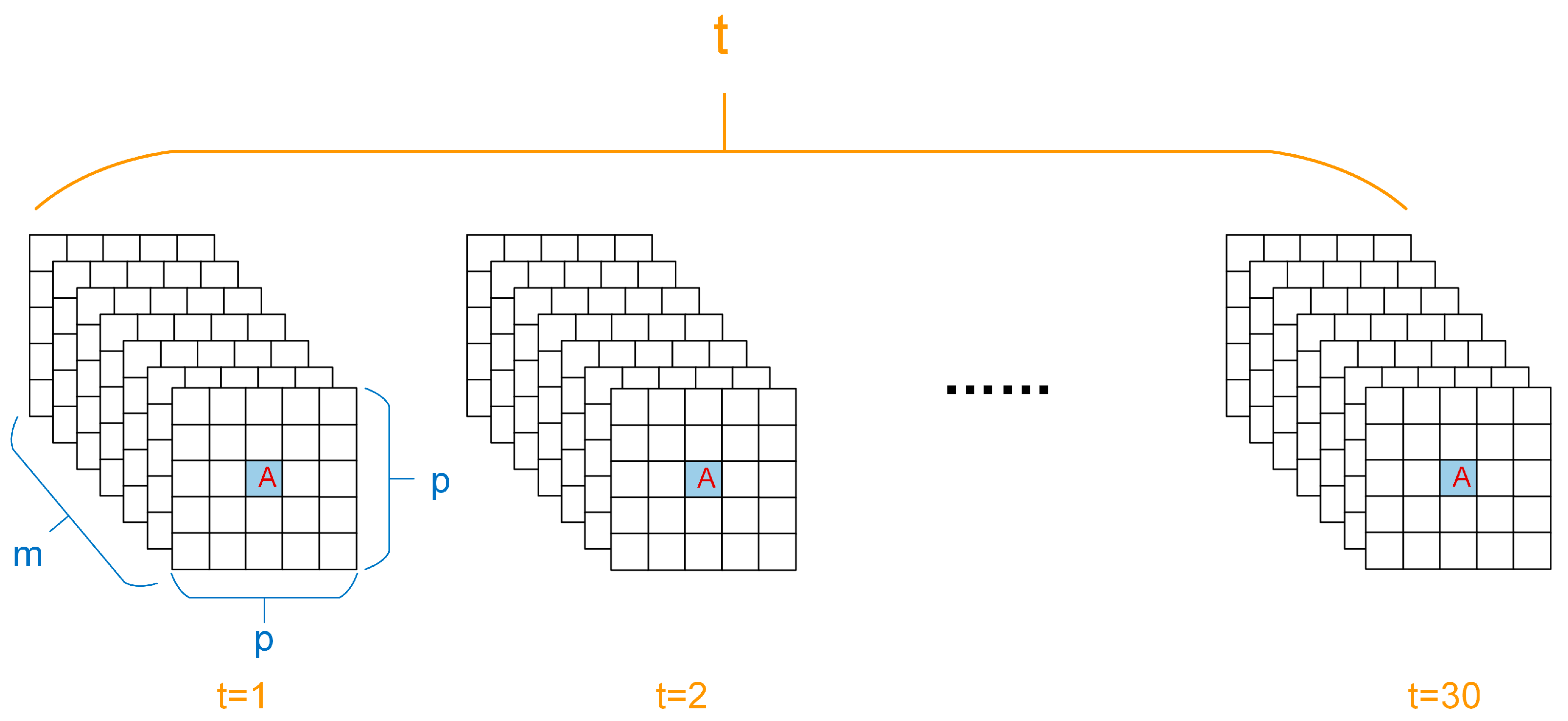
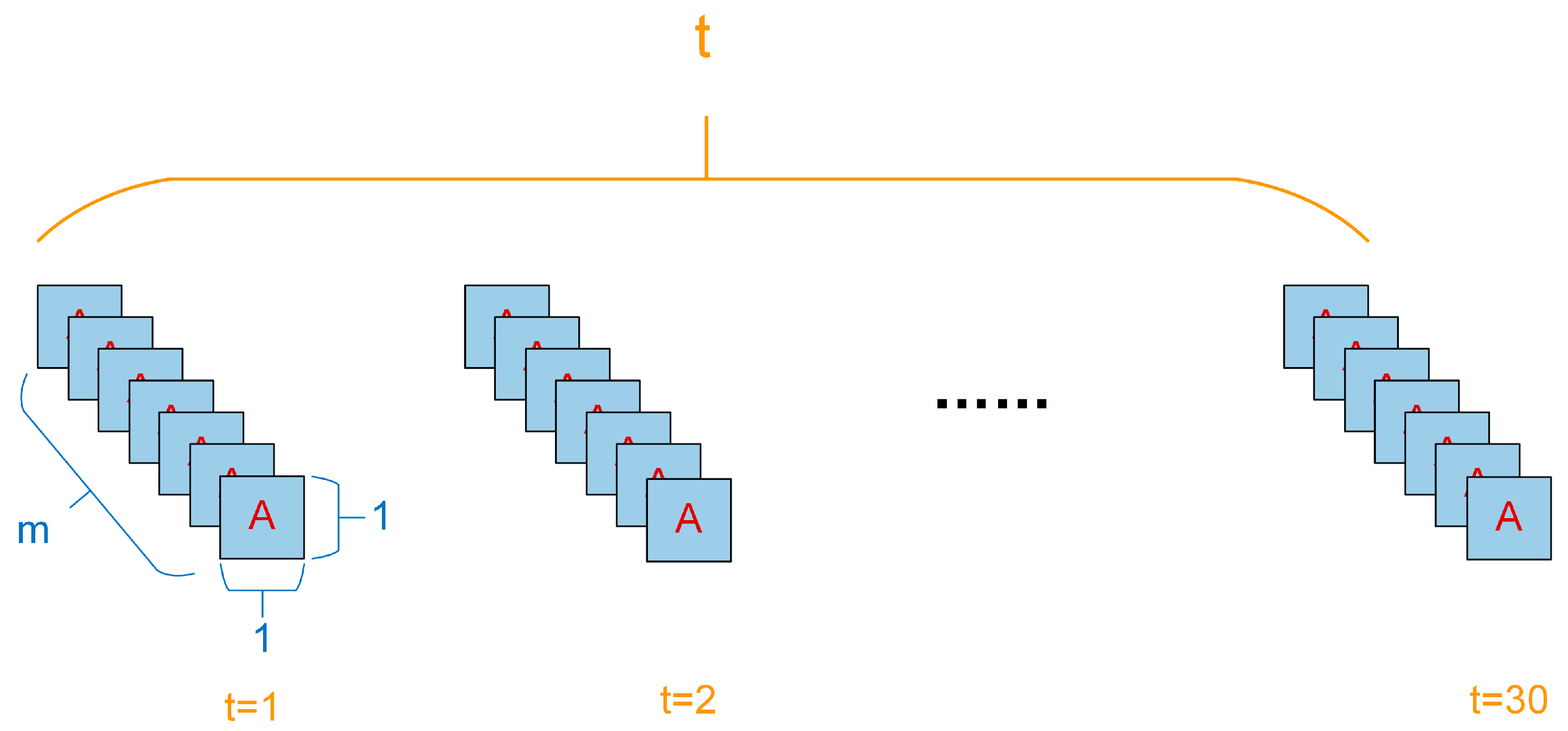
3.2.1. Patch-Based Strategy

In pixel-based image classification studies, images are commonly vectorized into separate pixels, disregarding the structural information between them [36]. Several studies have demonstrated that a patch-based strategy can significantly enhance classification accuracy [30,37]. Notably, a filter strategy exists within the patch-based method: a patch is only used for classification if 60% or more of its pixels belong to the same category as the central pixel [27]. In this study’s primary experiments, the filter strategy was not employed; however, we analyze its implications in the Discussion section.
Referring to existing research experiments, patch sizes of 1, 3, 5, 7, 9, 11, 13, 15, 17, 19, and 21 pixels were tested to determine the most suitable size. A patch size of 1 represents a pixel-based method. Figure 4 illustrates the schematic diagram of patch composition. The experiments involved moving the window from the image’s top-left corner of the image to the bottom-right corner, row by row, at the pixel level, as shown in Figure 5. Each patch overlapped with the subsequent pixel, thus capturing maximum information. The final result was a four-dimensional patch of time × width × height × channel, with the patch class corresponding to the central pixel’s class, as depicted in Figure 6 and Figure 7.

3.2.2. Models for Comparison

Six classifiers were evaluated in this classification study: a one-dimensional Convolutional Neural Network (Conv1d), a three-dimensional Convolutional Neural Network (Conv3d), a two-dimensional Convolutional Neural Network with a separate Long Short-Term Memory backend (Conv2d + LSTM) [28], and a two-dimensional Convolutional LSTM (ConvLSTM2d).
Random Forest is an ensemble learning method based on the bagging algorithm and consists of a set of decision trees. The integration of multiple decision trees enhances the generalization ability and stability of RF. Given its robustness against noise and reduced overfitting, RF is widely employed in research [38]. In this study, RF is implemented using Scikit-learn, with Grid-Search applied for parameters optimization based on references. A 10-fold cross-validation is used for training and evaluation. The final values for n_estimator and max_depth are 150 and 40, respectively, while other parameters maintain their default values.
A Convolutional Neural Network (CNN) is a classic image-processing algorithm. It excels at analyzing spatial structures within neighboring image blocks and efficiently handles multi-dimensional data through parameter sharing [28]. The CNN training process consists of two stages: forward propagation and back propagation. In the forward propagation stage, the input data traverses convolutional layers, pooling layers, and finally outputs the results through a fully connected layer. During back propagation, the model’s weights and biases are optimized using the gradient descent algorithm, which relies on the loss function. This study employed the categorical_crossentropy loss function, as described in Equation (1) [39].
L o s s = i = 1 n y i · log y ı ^
where n is the category of the classification, y ı is the actual category value of the sample, and y i ^ is the predicted category value of the sample.
This study employed two CNN models: Conv1d and Conv3d. Conv1d utilizes a one-dimensional convolutional kernel to extract information from sequences, while Conv3d processes time-series images more effectively by mining spatial and temporal information through 3D convolution and pooling operations [40,41]. These CNN models were combined with pooling layers, dropout, and a fully connected layer. The pooling layers spatially down-sample the feature map, condensing semantic information by monitoring abstract features and contextual information across scales to reduce computational resource consumption and overfitting risk. Dropout, an effective regularization technique, introduces stochasticity into the training process by randomly setting a portion of a layer’s output features to zero, thus mitigating the statistical noise effects. Lastly, the fully connected layer is responsible for classification [39].
To enhance efficiency, the classification models’ numerous parameters were empirically adjusted to explore potential network architectures. During the optimization of deep-learning classifiers, filter values of 32, 64, 128, and 256 were tested in different layer permutations. The effects of average pooling and maximum pooling were compared. Learning rates of 0.001 and 0.0001 and batch sizes of 32, 64, and 128 were assessed, with a final selection of a 0.0001 learning rate and a 64 batch size. The dropout_ratio was set to 0.5. The proposed deep-learning classifiers utilized the Adam optimizer with categorical cross-entropy loss function. Table 3 presents the main layers and output dimensions of the two CNNs. The input of Conv3d is patch-based, while the input of Conv1d is pixel-based.
RNN enhances the neural network’s analytical capabilities in the time dimension through loops in connections [23], making it a natural candidate for learning temporal information in time-series images [25]. Long Short-Term Memory (LSTM), a variant of the RNN, solves the long-term dependencies problem with a “gate” mechanism [24,42]. LSTM mainly comprises forget input and output gates. The forget gate decides the information to be removed from the previous moment [26]. This study employed an LSTM layer (unit = 30), a dropout layer, and a dense layer for classification. The input shape was t × m, and the output shape was n. The hyper-parameters were the same as those of CNNs.
In order to combine the advantages of feature extraction in both spatial and temporal dimensions using CNN and RNN, researchers have proposed two combinations: (1) A relatively loose combination where CNN and RNN are connected sequentially; (2) A more in-depth fusion called two-dimensional Convolutional LSTM (ConvLSTM2d). In the LSTM structure, the MLP layer is replaced with a convolutional layer so that LSTM can also handle spatial data structures [43]. This attempt was also practiced in this study by introducing Conv2d + LSTM and ConvLSTM2d. In the Conv2d + LSTM network, the time-distributed method was utilized to preserve the data’s temporal structure before inputting it into the LSTM module. The hyper-parameters were identical to those of the CNNs. The main layers and output shape of Conv2d + LSTM and ConvLSTM2d are shown in Table 4.
It has been suggested that convolutions perform local computations, while recurrent neural networks are better suited for capturing long-term dependencies in time-series data. Therefore, this study focused on comparing the differences among Conv2d + LSTM, ConvLSTM2d, and Conv3d. Conv1d, LSTM, and RF were also included for comparative analysis.

3.3. Evaluation

To evaluate the performance of different classifiers, we calculated the confusion matrix, kappa value, accuracy score, and classification report using Sklearn’s built-in functions. The classification report displayed the precision, recall, f1-score, and accuracy for each crop category. Based on this, we can evaluate different classification models from two perspectives: overall performance and single category performance.

3.4. Hardware Configuration and Software Environment

The hardware configuration involved in this study is Intel(R) Core(TM) i9-9900X CPU, 64 GB memory, and NVIDIA GeForce RTX 3090 GPU. For the software environment, the operating system is Windows 10, Python version 3.7.4, and the neural network model is built based on TensorFlow 1.15.4, Keras 2.3.1, and Sklearn 0.21.3.

4. Results and Analysis

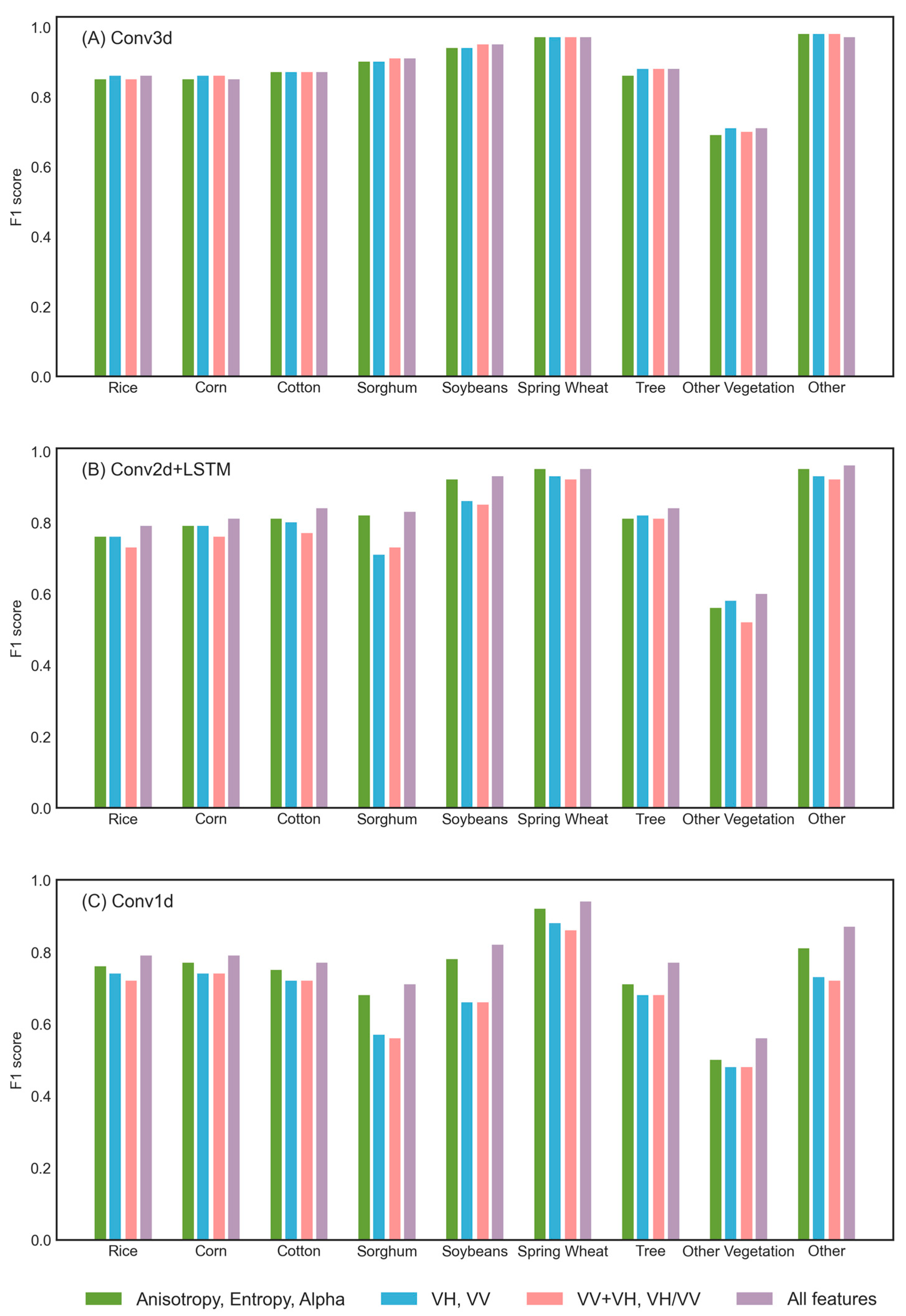
4.1. Patch-Based Strategy and Feature Importance Comparison

In the experiment, the patch strategy significantly improves the accuracy of the results. A pixel-based Conv3d achieves an accuracy of 77.6% and a kappa value of 0.747, while the patch-based Conv3d reaches 88.9% and 0.875, respectively. We also tested different patch sizes and concluded that the optimal size is 17. According to Figure 8, the classification effect does not change monotonically as the patch size increases. When the patch size is 3, the classification result is even inferior to the pixel-based Conv3d. An important turning point is reached when the patch size is nine. Beyond this point, increasing the patch size has less impact on optimizing the classification performance. The classification result reaches its peak when the patch size is 17 and starts to decrease when the patch size is larger than 17.
Feature selection serves as the foundation for image classification. In this study, the importance scores of the seven features used were calculated using Random Forest and ranked in descending order as follows: Anisotropy (0.210), Entropy (0.197), Alpha (0.178), VH (0.133), VV + VH (0.132), VV (0.099), and VH/VV (0.050). Table 5 displays the accuracy and kappa values for the three deep-learning models using different inputs. It can be seen that the highest accuracy is achieved for all three classifiers when utilizing all features. In Conv3d, the classification accuracy based on different inputs does not vary significantly. In Conv2d and Conv1d, the classification accuracy based on Anisotropy, Entropy, and Alpha is higher than those based on VH, VV, or VV + VH, VH/VV. Moreover, the classification results based on backscatter coefficients (VH, VV, or VV + VH, VH/VV) are similar.

4.2. Comparison among Models

A comparison of the classification performance of each classifier is shown in Table 6. Conv3d has the best overall performance, with the highest accuracy and kappa value among all others, and its relatively short training time is also noticeable. Conv2d + LSTM and ConvLSTM2d, which combine the virtues of CNN and RNN, also perform well, with slightly lower accuracy and kappa than Conv3d. Notably, Conv2d + LSTM has a short training time per epoch, while ConvLSTM2d takes longer to complete the training of an epoch but reaches a smooth position faster than Conv2d + LSTM. LSTM demonstrates the poorest classification performance and the longest training time. Conversely, Conv1d yields slightly better classification results than the former with the shortest training time. In general, Conv1d and LSTM, which utilize only the temporal information, produce inferior classification results and underperform compared to Random Forest. Conv3d, Conv2d + LSTM, and ConvLSTM2d fuse both spatial and temporal information and therefore obtain more desirable outcomes than RF. In addition, the networks using LSTM units exhibit increased curve roughness during training, leading to an extended training time.

4.3. Classification Results for Each Crop Category

As Conv3d exhibited the best performance, the analysis for each crop category is based on Conv3d. Table 7 presents the confusion matrix for the multi-class crop classification task within the study area, encompassing indicators such as precision, recall, F1-score overall accuracy and kappa.
The classification performance for the “Spring Wheat” and “Other” categories is observed to be the best. The “Other” category mainly includes water and developed land, which exhibit significantly distinct scattering characteristics compared to other classes. This justifies the high precision (0.95), recall (1.00), and F1-score (0.97) achieved for the “Other” category. The classification performance for “Cotton” and “Soybeans” is also desirable with an accuracy of 0.88, while the overall performance for the “Rice”, “Corn”, “Sorghum”, and “Tree” categories is deemed acceptable. The poorest classification result is found in the “Other Vegetation” class, which can be attributed to the reclassification process. During this process, 32 feature classes based on the CDL classification criteria, including rye, oats, millet, canola, sugarcane, watermelons, etc., were categorized as “Other Vegetation”. These species exhibit a wide range of vegetation morphologies and scattering characteristics; therefore, this category is prone to confusion with other classes during classification.
The classification results for individual crop categories exhibit slight variations, which can be attributed to the following reasons: From a spatial distribution perspective, the distribution of the “Soybeans”, “Sorghum”, and “Tree” categories is fragmented, with curved plot boundary lines. The “Tree” category, in particular, consists of numerous thin strips, making it susceptible to misjudgment at the boundary lines. Furthermore, due to the superior spatial resolution of Sentinel images (10 m) compared to CDL (30 m), more detailed prediction results might be considered as wrong. In contrast, rice, corn, cotton, and spring wheat are mainly distributed in squares with regular boundaries, allowing for better spatial distinction. However, rice, corn, and cotton also exhibit partial spatial mixing, which accounts for their misclassification in the confusion matrix. From a crop calendar perspective (Figure 3), corn and sorghum, as well as spring wheat and spring oats (reclassified as “Other Vegetation”), share some common characteristics, increasing the possibility of classification errors.

5. Discussion

5.1. Analysis of Feature Importance

One of this study’s central aims is to evaluate the performance of polarimetric decomposition features compared to the commonly used backscatter coefficient. However, according to the calculations, the performance of each feature varies across different classifiers. To investigate the underlying mechanism, we averaged the feature values of all samples in the dataset for further analysis. Figure 9 presents the trend of feature values for different crop categories. It is evident that Anisotropy, Entropy, Alpha, and VH/VV enhance the distinguishability of crop categories over time. In contrast, the trends of different crop categories are more similar under VH, VV, and VH + VV. This observation aligns with the results in Table 5, indicating that polarization decomposition features are more favorable for classification. Although VH/VV improves the distinguishability of crop categories, it does not stand out in the classification results, presumably because of the insufficient contribution of VH + VV. Consequently, the combination of the two is inferior to the polarization decomposition features.
The introduction of polarization decomposition features (Anisotropy, Entropy, and Alpha) can provide a more comprehensive analysis of the microwave scattering characteristics of crops. Entropy indicates the scattering randomness of the feature, with values ranging from 0 to 1. A higher value signifies greater randomness. Alpha indicates the scattering mechanism of the feature, while Anisotropy complements Entropy by indicating the strength relationship between the weaker scattering components other than the strongest scattering mechanism [12,13]. Combining the crop calendar (Figure 3) and Figure 9, the following patterns can be found:
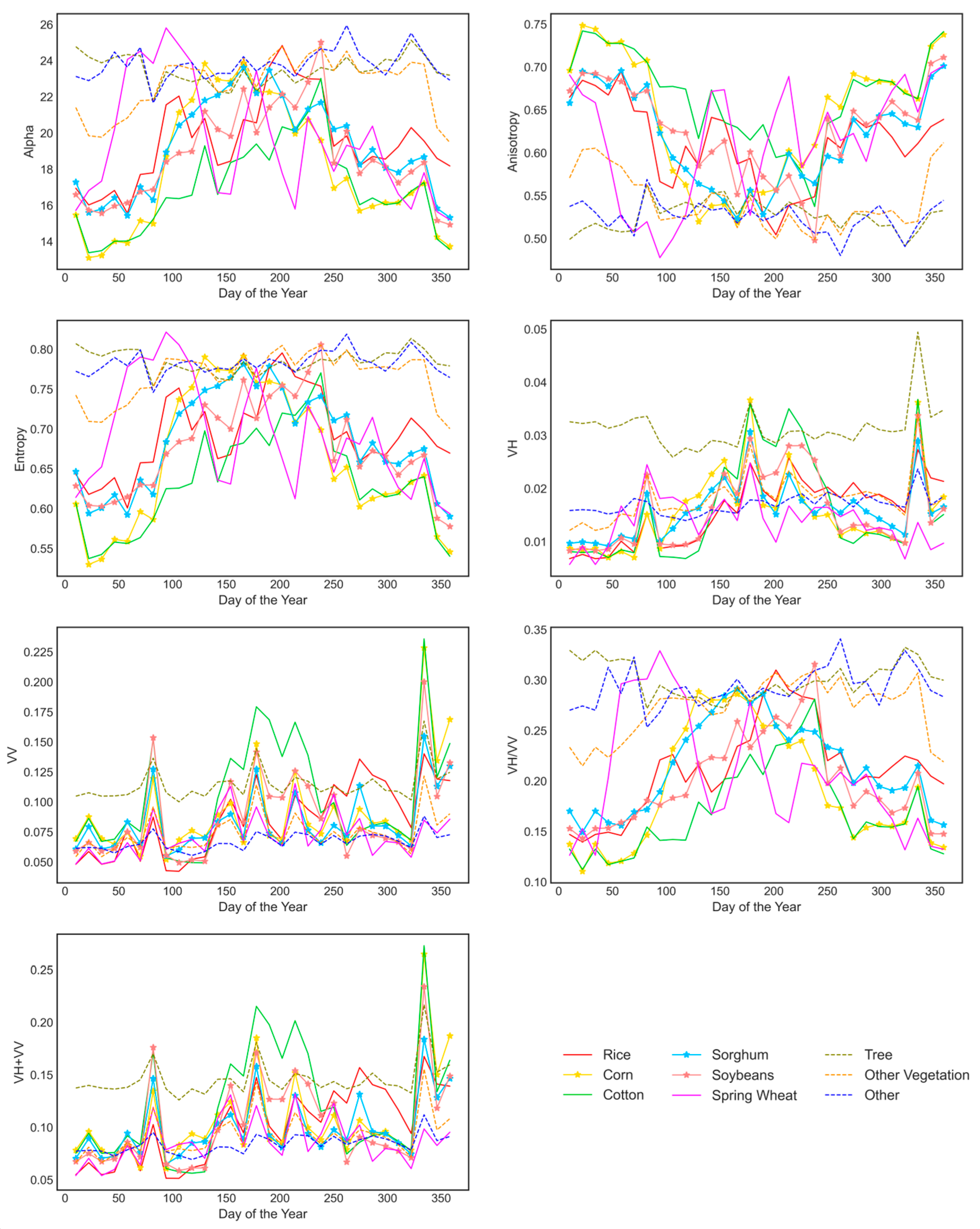
  • The “Other” and “Tree” categories exhibit minimal fluctuations throughout the year, with each feature displaying distinct differences compared to other categories. This can be attributed to the high surface roughness of the “Tree” category, where the canopy, trunk and ground surface contribute to a complex multiple scattering mechanism. As a result, Anisotropy, Entropy, Alpha, and backscatter coefficients remain consistently high. In contrast, the “Other” category mainly comprises water and built-up areas, leading to stable scattering characteristics.
  • “Rice”, “Spring Wheat”, and “Cotton” show differences in each feature. The backscatter coefficient is strongly influenced by water content and surface roughness. “Rice” demands frequent irrigation during its growing period, resulting in lower backscatter coefficients. Crops with significant vertical structure typically have higher horizontal polarization backscatter coefficients, “Spring Wheat” possesses a weaker vertical structure compared to “Cotton” and “Sorghum”, leading to lower backscatter coefficients. The polarization decomposition features vary with the changes in crop morphology. The Entropy and Alpha of “Spring Wheat” change earlier because of early sowing. With the increase in leaves, the surface scattering intensifies rapidly, enhancing polarization complexity and raising Entropy. During the late growth period, Entropy and Alpha do not decrease as rapidly as VH and VV. It is hypothesized that the wheat spike acts as a new scatterer, increasing randomness and leading to higher Entropy [44].
  • The microwave scattering characteristics of “Corn”, “Sorghum,” and “Soybean” exhibit high similarity in the VH, VV, and VH + VV channels. However, distinctions are noticeable in their polarization decomposition features. During the early growth stage, “Corn” presents lower Entropy and Alpha values compared to “Sorghum” and “Soybean”. This discrepancy is likely attributed to the larger row and plant spacing in “Corn”, resulting in a higher contribution of soil information to the signal, thereby differentiating it from the other crops.
  • In VH, VV, and VH + VV polarization channels, the “Other Vegetation” category tends to be easily confused with other categories due to its diverse constituents exhibiting mixed scattering characteristics. Nevertheless, distinctions in Anisotropy, Entropy, and Alpha are observed, which could be attributed to the consistently high complexity of this category throughout the growth period, resulting in elevated Entropy values.
Comparing the F1 scores for each category using different features (Figure 10), it is found that Anisotropy, Entropy, and Alpha can improve the classification of ambiguous categories such as “Sorghum” and “Soybean”. However, the performance of polarization decomposition features for “Other Vegetation” remains unsatisfactory. It is hypothesized that while these features improve differentiation from the main crops, they concurrently decrease distinction from trees. In the backscatter coefficients, the difference between this category and “Tree” is obvious. Therefore, the classification based on all features can achieve the best results.

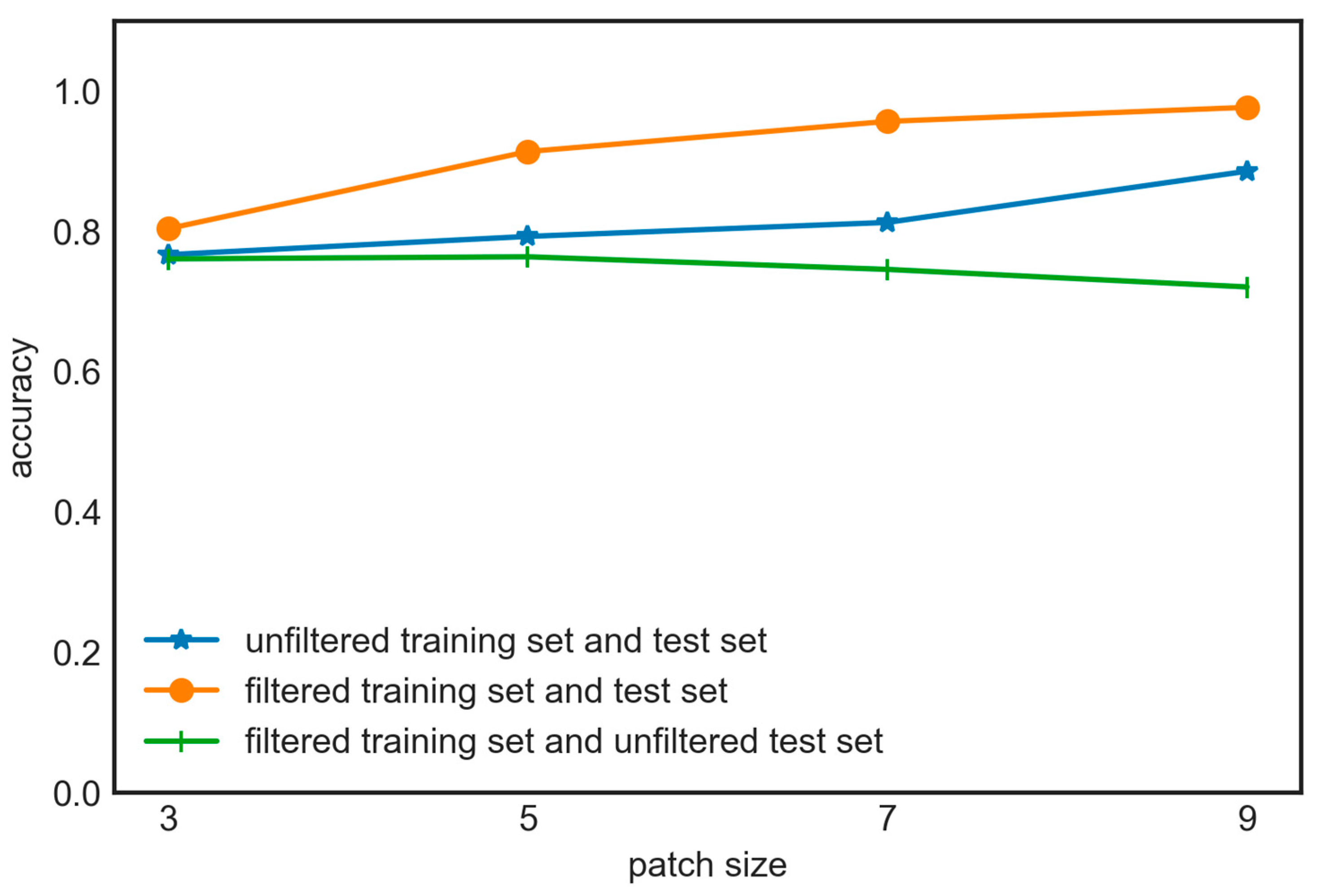
5.2. Influence of Patch Size and Dataset Filtering

The impact of patch size on classification results is another intriguing aspect to explore. Figure 11 spatially visualizes the pattern exhibited in Figure 5. In general, the following observations can be made: (1) In areas with regular distribution, classification errors are less frequent for different patch sizes. As illustrated in Figure 9, the “Corn” plots with large area distribution have minimal black pixels, indicating fewer errors. (2) At the boundaries of regularly distributed cropland plots, the probability of classification errors diminishes as the patch size increases. Specifically, when the patch size is greater than or equal to nine, the predicted categories align with the surrounding large-area crops. However, with smaller patch sizes, the predicted categories may correspond to any of the surrounding crop types. (3) In areas where multiple crop types intermingled on a small scale, patch sizes of nine and above have significantly better performance. Unexpectedly, the probability of classification errors is higher than the pixel-based method when patch size takes the value of three.
We can explain the rationale for the above phenomenon in terms of patch size:
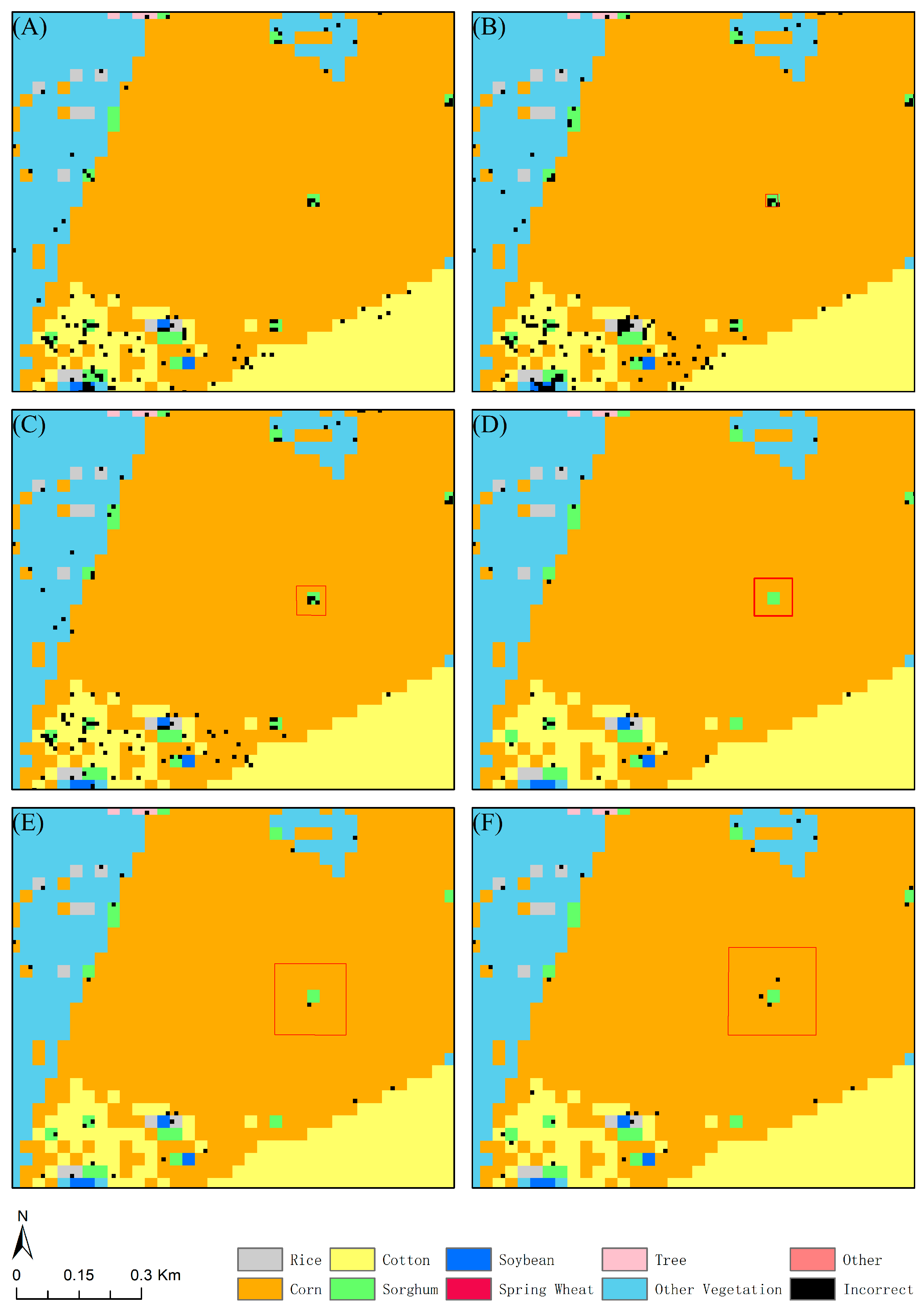
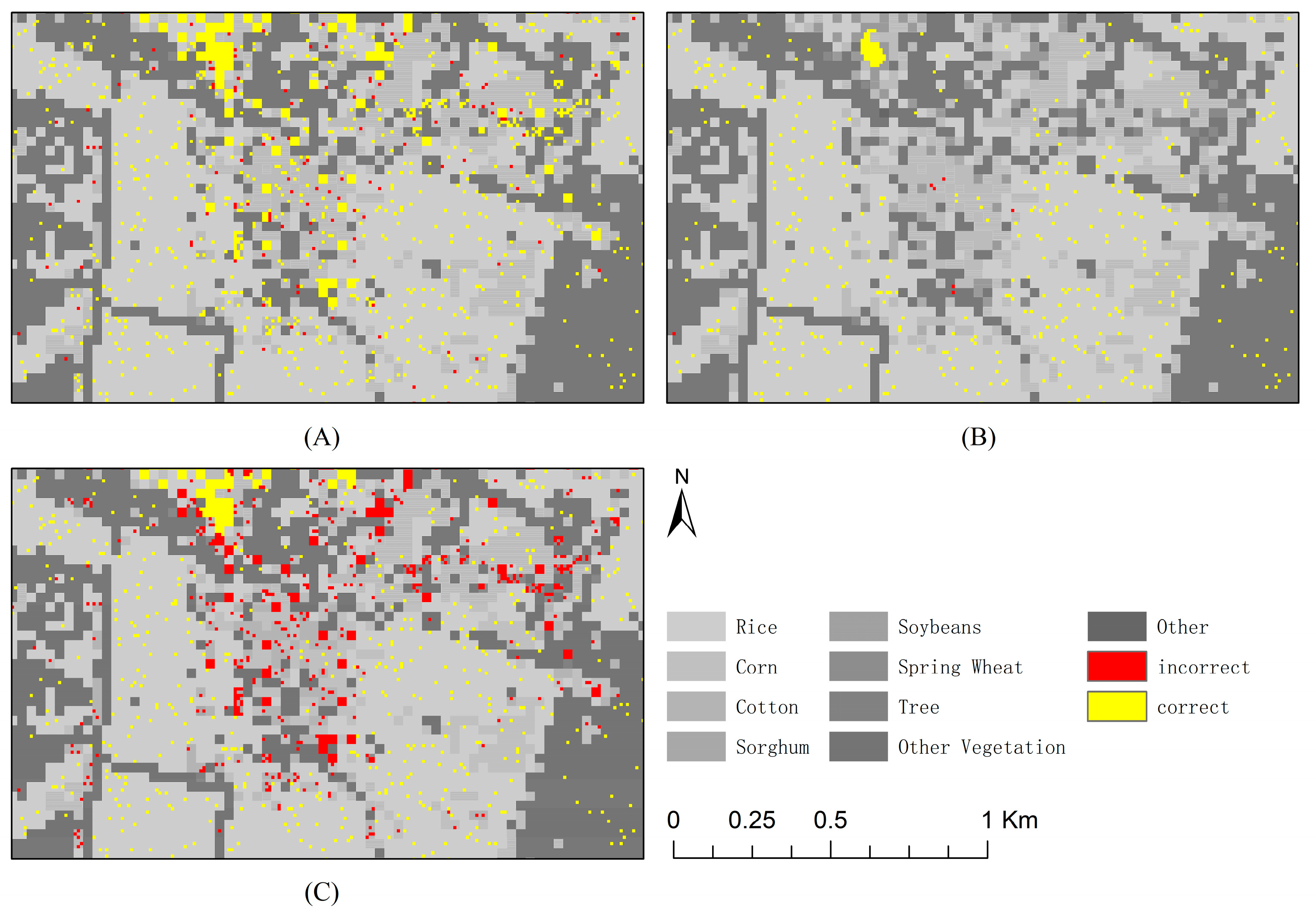
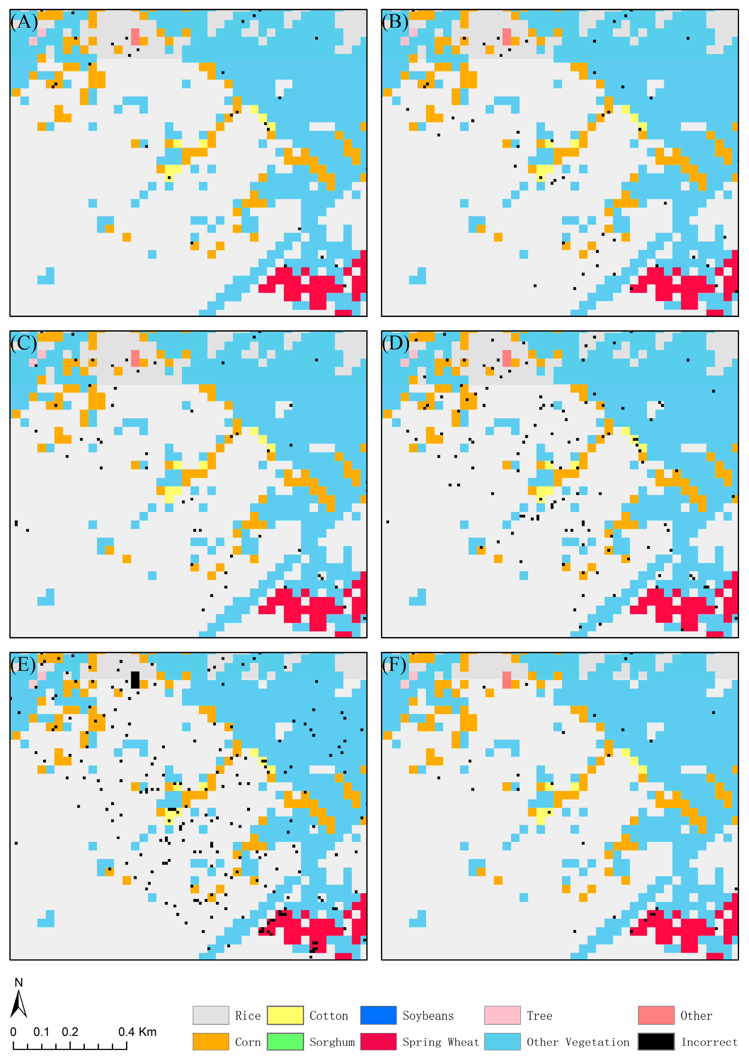
  • In the absence of a patch strategy, the classification model’s predictions exhibit substantial randomness due to the lack of consideration for the surrounding information.
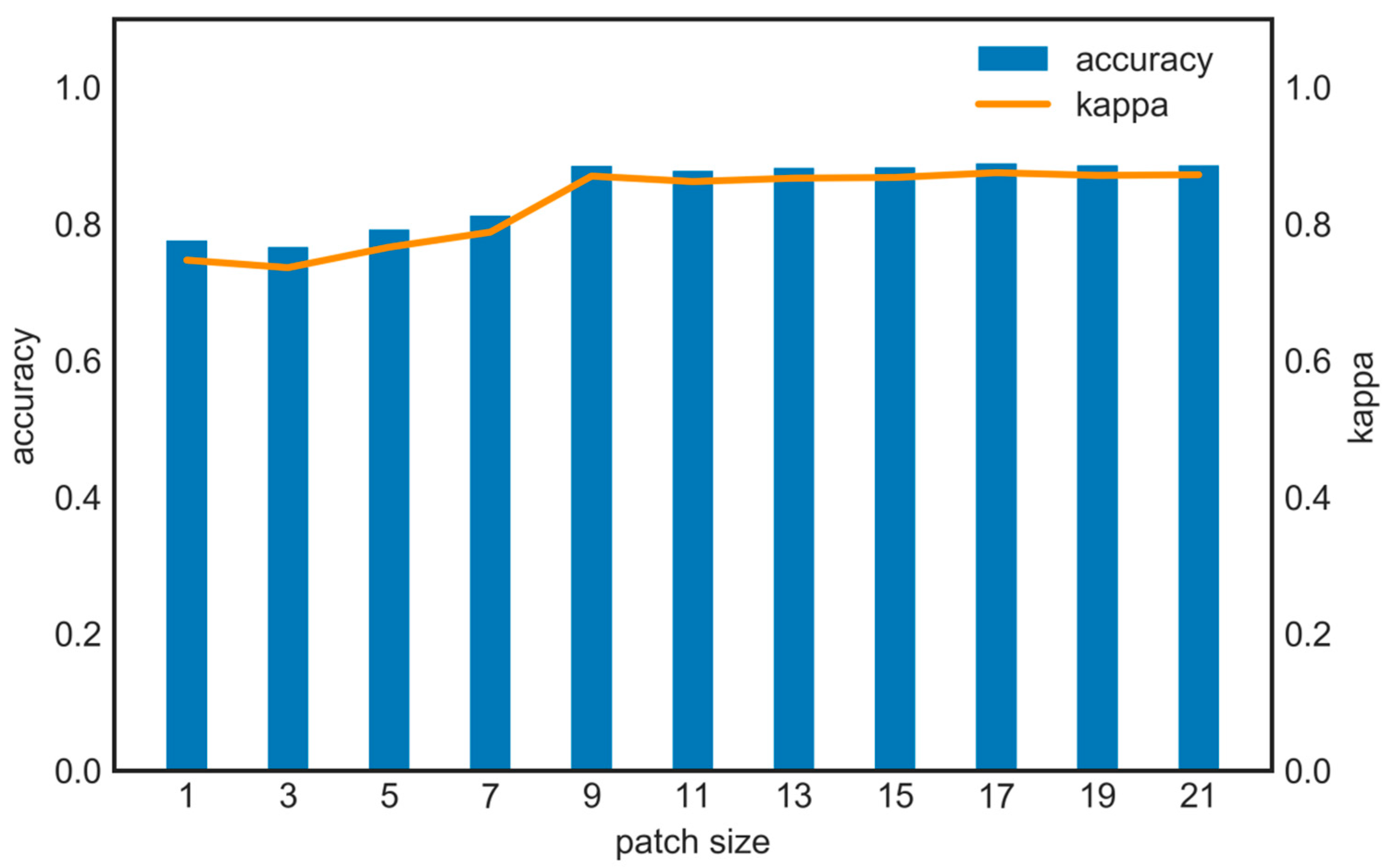
  • When employing smaller patch sizes, the coverage is limited, and the surrounding crops with a small area will occupy a relatively large proportion of the patch, increasing the spatial heterogeneity. It was found that the patch strategy proves effective when less than 50% of pixels within the patch differ from the central pixel’s category. However, when the ratio exceeds 87.5%, the patch strategy negatively impacts classification [45]. Meanwhile, smaller patches also contained limited spatial information, hindering the CNN’s ability to accurately discern crop-category distribution patterns in space. Therefore, smaller patch sizes may result in higher classification errors and increased randomness in model predictions.
  • As the patch size increases, the influence of surrounding small-scale crops decreases, resulting in reduced spatial heterogeneity. This allows for the acquisition of more information on the distribution structure because of the broader coverage, ultimately enhancing the classification performance.
  • When the patch is excessively large, it causes unnecessary computational resources consumption and introduces irrelevant information that could interfere with the classification process, leading to a slight decrease in accuracy. At the same time, an overly large patch may result in excessive smoothing, ignoring small or linearly distributed categories around patchy crop categories, affecting the precision and certainty of the boundaries [46].
In order to optimize the classification results, a filtering strategy is applied to reduce the impact of interfering information within patches: This strategy is employed when 60% or more of the pixels in a patch belong to the same category as the central pixel, allowing the patch to be used for classification [47]. We explored the effectiveness of this method in two cases: (1) utilizing the filtered training and test sets and (2) employing the filtered training set and unfiltered test set. These were compared to the case where neither the training nor test sets were filtered. We practiced with patch sizes of three, five, seven, and nine. The sample size for different cases when patch size equals nine is shown in Table 8. According to Figure 12, the filtering strategy effectively improves accuracy. However, when the model trained on the filtered training set is applied to the unfiltered test set, its performance is inferior to that of the model without the filtering method, as the model has not acquired the relevant knowledge. We present the spatial comparison of the above cases in Figure 13, using a patch size of nine. It is evident that the filtering strategy obtains a sample set with low interference information by discarding samples from regions with complex crop-type distribution. When the model based on the filtering strategy is used to classify such intricate regions, fewer classification errors occur. Furthermore, if the study area’s distribution is complex, some categories may not retain enough training samples under the filtering conditions. In this study, a patch size of nine represents the upper limit. Therefore, we conclude that the filtering strategy can improve the classification performance, but with certain limitations in its application.

5.3. Discussion of the Classification Performance of Each Model

The spatial representation of the classification results is shown in Figure 14. Regardless of the classifier used, errors are more common in areas where different categories overlap. These errors can be attributed to the following factors: (1) Crop boundaries may contain mixed species, leading to confusion in scattering properties. (2) Conv3d, Conv2d + LSTM, and ConvLSTM2d classifiers all used the patch strategy, which, while supplementing the spatial information, may also lead to excessive smoothing and ignoring small or linearly distributed categories around patchy crop categories, thus affecting the certainty of the boundaries. (3) The spatial resolution of CDL data as ground truth is 30 m, which is three times the SAR data used for classification, potentially causing more detailed boundary information to be misinterpreted as classification errors. Specifically, Conv3d tends to make mistakes in small-area crops: (1) If a sporadically distributed crop is situated near a large area of the same crop, Conv3d is prone to incorrectly incorporate the smaller crop into the larger one’s class, resulting in a visually inflated effect. (2) In crop plots with multiple intermingled classes, Conv3d is likely to produce more sporadic classification errors due to the influence of neighboring pixels. We hypothesize that the patch strategy exacerbates these classification errors to some extent. Furthermore, the classification results of Conv2d + LSTM and ConvLSTM2d are relatively similar. In addition to misclassifications at boundaries, both classifiers are prone to making mistakes within large plots of the same type, resulting in a salt-and-pepper phenomenon. In the case of Conv1d and LSTM, where only time-series data are utilized, classification errors become more obvious, with many small crops remaining undistinguished. Conversely, RF performs well, with minimal errors at boundaries and within large plots.

6. Conclusions

Among the evaluated classifiers, Conv3d achieved the best performance. Conv2d + LSTM and ConvLSTM2d, which combine CNN and RNN to extract spatial and temporal information performed well, too. In selecting classification features, Anisotropy, Entropy, and Alpha which extracted by polarization decomposition delivered desirable classification results, especially in the time-series analysis. These features outperformed backscatter coefficients in distinguishing different crops. The patch strategy significantly improved classification accuracy, with the 17 × 17 patch size optimally capturing the spatial correlations between central and peripheral pixels.
Our research has verified the practical value of the patch strategy in SAR image classification and the potential of polarization decomposition features for crop type classification. Based on the accuracy of the test dataset, our crop type classification method demonstrates significant application potential in practice.
In future, introducing high-resolution remote sensing images can improve classification accuracy and optimize the parcel boundary classification. Furthermore, because of the limitation of dual-polarization SAR data, full-polarization data can be considered for richer polarization information.

Author Contributions

Conceptualization, Y.L. and Z.S.; data analysis, methodology, and original draft preparation, Y.L.; review and editing, X.P. and Z.S. All authors have read and agreed to the published version of the manuscript.

Funding

This research received no external funding.

Data Availability Statement

The data that support the findings of this study are available upon reasonable request from the authors.

Conflicts of Interest

The authors declare no conflict of interest.

References

  1. Gella, G.W.; Bijker, W.; Belgiu, M. Mapping Crop Types in Complex Farming Areas Using SAR Imagery with Dynamic Time Warping. ISPRS J. Photogramm. Remote Sens. 2021, 175, 171–183. [Google Scholar] [CrossRef]
  2. Buckley, C.; Carney, P. The Potential to Reduce the Risk of Diffuse Pollution from Agriculture while Improving Economic Performance at Farm Level. Environ. Sci. Policy 2013, 25, 118–126. [Google Scholar] [CrossRef] [Green Version]
  3. Kussul, N.; Lavreniuk, M.; Skakun, S.; Shelestov, A. Deep Learning Classification of Land Cover and Crop Types Using Remote Sensing Data. IEEE Geosci. Remote Sens. Lett. 2017, 14, 778–782. [Google Scholar] [CrossRef]
  4. Van Tricht, K.; Gobin, A.; Gilliams, S.; Piccard, I. Synergistic Use of Radar Sentinel-1 and Optical Sentinel-2 Imagery for Crop Mapping: A Case Study for Belgium. Remote Sens. 2018, 10, 1642. [Google Scholar] [CrossRef] [Green Version]
  5. Wang, D.; Zhang, H. Inverse-Category-Frequency Based Supervised Term Weighting Schemes for Text Categorization. J. Inf. Sci. Eng. 2013, 29, 209–225. [Google Scholar]
  6. Turkoglu, M.O.; D’Aronco, S.; Perich, G.; Liebisch, F.; Streit, C.; Schindler, K.; Wegner, J.D. Crop Mapping from Image Time Series: Deep Learning with Multi-Scale Label Hierarchies. Remote Sens. Environ. 2021, 264, 112603. [Google Scholar] [CrossRef]
  7. Johnson, D.M.; Mueller, R. Pre- and within-Season Crop Type Classification Trained with Archival Land Cover Information. Remote Sens. Environ. 2021, 264, 112576. [Google Scholar] [CrossRef]
  8. Bargiel, D. A New Method for Crop Classification Combining Time Series of Radar Images and Crop Phenology Information. Remote Sens. Environ. 2017, 198, 369–383. [Google Scholar] [CrossRef]
  9. Guo, Y.; Jia, X.; Paull, D.; Benediktsson, J.A. Nomination-Favoured Opinion Pool for optical-SAR-synergistic Rice Mapping in Face of Weakened Flooding Signals. ISPRS J. Photogramm. Remote Sens. 2019, 155, 187–205. [Google Scholar] [CrossRef]
  10. Campbell, J.B.; Wynne, R.H. Introduction to Remote Sensing; Guilford Press: New York, NY, USA, 2011. [Google Scholar]
  11. Tufail, R.; Ahmad, A.; Javed, M.A.; Ahmad, S.R. A Machine Learning Approach for Accurate Crop Type Mapping Using Combined SAR and Optical Time Series Data. Adv. Space Res. 2022, 69, 331–346. [Google Scholar] [CrossRef]
  12. Cloude, S.R.; Pottier, E. A Review of Target Decomposition Theorems in Radar Polarimetry. IEEE Trans. Geosci. Remote Sens. 1996, 34, 498–518. [Google Scholar] [CrossRef]
  13. Cloude, S.R.; Pottier, E. An Entropy Based Classification Scheme for Land Applications of Polarimetric SAR. IEEE Trans. Geosci. Remote Sens. 1997, 35, 68–78. [Google Scholar] [CrossRef]
  14. Freeman, A.; Durden, S.L. A Three-Component Scattering Model for Polarimetric SAR Data. IEEE Trans. Geosci. Remote Sens. 1998, 36, 963–973. [Google Scholar] [CrossRef] [Green Version]
  15. Huynen, J.R. Phenomenological Theory of Radar Targets. Ph.D. Thesis, Faculty of Electrical Engineering, Mathematics and Computer Science, Delft, The Netherlands, 1970. [Google Scholar]
  16. Hoang, H.K.; Bernier, M.; Duchesne, S.; Tran, Y.M. Rice Mapping Using RADARSAT-2 Dual-And Quad-Pol Data in a Complex Land-Use Watershed: Cau River Basin (Vietnam). IEEE J. Sel. Top. Appl. Earth Obs. Remote Sens. 2016, 9, 3082–3096. [Google Scholar] [CrossRef]
  17. Lopez-Sanchez, J.M.; Ballester-Berman, J.D.; Hajnsek, I. First Results of Rice Monitoring Practices in Spain by Means of Time Series of TerraSAR-X Dual-Pol Images. IEEE J. Sel. Top. Appl. Earth Obs. Remote Sens. 2010, 4, 412–422. [Google Scholar] [CrossRef]
  18. Shao, Y.; Fan, X.; Liu, H.; Xiao, J.; Ross, S.; Brisco, B.; Brown, R.; Staples, G. Rice Monitoring and Production Estimation Using Multitemporal RADARSAT. Remote Sens. Environ. 2001, 76, 310–325. [Google Scholar] [CrossRef]
  19. Lasko, K.; Vadrevu, K.P.; Tran, V.T.; Justice, C. Mapping Double and Single Crop Paddy Rice with Sentinel-1A at Varying Spatial Scales and Polarizations in Hanoi, Vietnam. IEEE J. Sel. Top. Appl. Earth Obs. Remote Sens. 2018, 11, 498–512. [Google Scholar] [CrossRef]
  20. Phan, A.; NHa, D.; DMan, C.; TNguyen, T.; QBui, H.; TNNguyen, T. Rapid Assessment of Flood Inundation and Damaged Rice Area in Red River Delta from Sentinel 1A Imagery. Remote Sens. 2019, 11, 2034. [Google Scholar] [CrossRef] [Green Version]
  21. Ndikumana, E.; Ho Tong Minh, D.; Baghdadi, N.; Courault, D.; Hossard, L. Deep Recurrent Neural Network for Agricultural Classification Using Multitemporal SAR Sentinel-1 for Camargue, France. Remote Sens. 2018, 10, 1217. [Google Scholar] [CrossRef] [Green Version]
  22. Zhang, M.; Lin, H.; Wang, G.; Sun, H.; Fu, J. Mapping Paddy Rice Using a Convolutional Neural Network (CNN) with Landsat 8 Datasets in the Dongting Lake Area, China. Remote Sens. 2018, 10, 1840. [Google Scholar] [CrossRef] [Green Version]
  23. Connor, J.T.; Martin, R.D.; Atlas, L.E. Recurrent Neural Networks and Robust Time Series Prediction. IEEE Trans. Neural Netw. 1994, 5, 240–254. [Google Scholar] [CrossRef] [Green Version]
  24. Hochreiter, S.; Schmidhuber, J. Long Short-Term Memory. Neural Comput. 1997, 9, 1735–1780. [Google Scholar] [CrossRef] [PubMed]
  25. Mou, L.; Bruzzone, L.; Zhu, X.X. Learning Spectral-Spatial-Temporal Features Via a Recurrent Convolutional Neural Network for Change Detection in Multispectral Imagery. IEEE Trans. Geosci. Remote Sens. 2018, 57, 924–935. [Google Scholar] [CrossRef] [Green Version]
  26. Qiao, M.; He, X.; Cheng, X.; Li, P.; Luo, H.; Zhang, L.; Tian, Z. Crop Yield Prediction from Multi-Spectral, Multi-Temporal Remotely Sensed Imagery Using Recurrent 3D Convolutional Neural Networks. Int. J. Appl. Earth Obs. Geoinf. 2021, 102, 102436. [Google Scholar] [CrossRef]
  27. Sharma, A.; Liu, X.; Yang, X.; Shi, D. A Patch-Based Convolutional Neural Network for Remote Sensing Image Classification. Neural Netw. 2017, 95, 19–28. [Google Scholar] [CrossRef]
  28. Thorp, K.R.; Drajat, D. Deep Machine Learning with Sentinel Satellite Data to Map Paddy Rice Production Stages across West Java, Indonesia. Remote Sens. Environ. 2021, 265, 112679. [Google Scholar] [CrossRef]
  29. Kussul, N.; Lemoine, G.; Gallego, F.J.; Skakun, S.V.; Lavreniuk, M.; Shelestov, A.Y. Parcel-Based Crop Classification in Ukraine Using Landsat-8 Data and Sentinel-1A Data. IEEE J. Sel. Top. Appl. Earth Obs. Remote Sens. 2016, 9, 2500–2508. [Google Scholar] [CrossRef]
  30. Carranza-García, M.; García-Gutiérrez, J.; Riquelme, J.C. A Framework for Evaluating Land Use and Land Cover Classification Using Convolutional Neural Networks. Remote Sens. 2019, 11, 274. [Google Scholar] [CrossRef] [Green Version]
  31. Gillespie, T.J.; Brisco, B.; Brown, R.J.; Sofko, G.J. Radar Detection of a Dew Event in Wheat. Remote Sens. Environ. 1990, 33, 151–156. [Google Scholar] [CrossRef]
  32. Wei, P.; Chai, D.; Lin, T.; Tang, C.; Du, M.; Huang, J. Large-Scale Rice Mapping under Different Years Based on Time-Series Sentinel-1 Images Using Deep Semantic Segmentation Model. ISPRS J. Photogramm. Remote Sens. 2021, 174, 198–214. [Google Scholar] [CrossRef]
  33. Xu, J.; Zhu, Y.; Zhong, R.; Lin, Z.; Xu, J.; Jiang, H.; Huang, J.; Li, H.; Lin, T. DeepCropMapping: A Multi-Temporal Deep Learning Approach with Improved Spatial Generalizability for Dynamic Corn and Soybean Mapping. Remote Sens. Environ. 2020, 247, 111946. [Google Scholar] [CrossRef]
  34. Zhong, L.; Gong, P.; Biging, G.S. Efficient Corn and Soybean Mapping with Temporal Extendability: A Multi-Year Experiment Using Landsat Imagery. Remote Sens. Environ. 2014, 140, 1–13. [Google Scholar] [CrossRef]
  35. Filipponi, F. Sentinel-1 GRD Preprocessing Workflow. Proceedings 2019, 18, 11. [Google Scholar]
  36. Nasirzadehdizaji, R.; Balik Sanli, F.; Abdikan, S.; Cakir, Z.; Sekertekin, A.; Ustuner, M. Sensitivity Analysis of Multi-Temporal Sentinel-1 SAR Parameters to Crop Height and Canopy Coverage. Appl. Sci. 2019, 9, 655. [Google Scholar] [CrossRef] [Green Version]
  37. Zhang, X.; Ding, Q.; Luo, H.; Hui, B.; Chang, Z.; Zhang, J. Infrared Small Target Detection Based on an Image-Patch Tensor Model. Infrared Phys. Technol. 2019, 99, 55–63. [Google Scholar] [CrossRef]
  38. Kim, W.; Lee, D.; Kim, Y.; Kim, T.; Lee, H. Path Detection for Autonomous Traveling in Orchards Using Patch-Based CNN. Comput. Electron. Agric. 2020, 175, 105620. [Google Scholar] [CrossRef]
  39. Dietterich, T.G. An Experimental Comparison of Three Methods for Constructing Ensembles of Decision Trees: Bagging, Boosting and Randomization. Mach Learn. 1998, 32, 1–22. [Google Scholar]
  40. Kattenborn, T.; Leitloff, J.; Schiefer, F.; Hinz, S. Review on Convolutional Neural Networks (CNN) in Vegetation Remote Sensing. ISPRS J. Photogramm. Remote Sens. 2021, 173, 24–49. [Google Scholar] [CrossRef]
  41. Ji, S.; Zhang, C.; Xu, A.; Shi, Y.; Duan, Y. 3D Convolutional Neural Networks for Crop Classification with Multi-Temporal Remote Sensing Images. Remote Sens. 2018, 10, 75. [Google Scholar] [CrossRef] [Green Version]
  42. Zhang, B.; Zhao, L.; Zhang, X. Three-Dimensional Convolutional Neural Network Model for Tree Species Classification Using Airborne Hyperspectral Images. Remote Sens. Environ. 2020, 247, 111938. [Google Scholar] [CrossRef]
  43. Rußwurm, M.; Korner, M. Temporal Vegetation Modelling Using Long Short-Term Memory Networks for Crop Identification from Medium-Resolution Multi-Spectral Satellite Images. In Proceedings of the 2017 IEEE Conference on Computer Vision and Pattern Recognition Workshops (CVPRW), Honolulu, HI, USA, 21–26 July 2017. [Google Scholar]
  44. Shi, X.; Chen, Z.; Wang, H.; Yeung, D.; Wong, W.; Woo, W. Convolutional LSTM Network: A Machine Learning Approach for Precipitation Nowcasting. Adv. Neural Inf. Process. Syst. 2015, 28, 802–810. [Google Scholar]
  45. Ding, Y.P. Dryland Crop Classification and Acreage Estimation Based on Microwave Remote Sensing; Chinese Academy of Agricultural Science: Beijing, China, 2013. [Google Scholar]
  46. Song, H.; Kim, Y.; Kim, Y. A Patch-Based Light Convolutional Neural Network for Land-Cover Mapping Using Landsat-8 Images. Remote Sens. 2019, 11, 114. [Google Scholar] [CrossRef] [Green Version]
  47. Jiang, T.; Wang, X. Convolutional Neural Network for GF-2 Image Stand Type Classification. J. Beijing For. Univ. 2019, 41, 20–29. [Google Scholar]
Figure 1. Flowchart.
Remotesensing 15 03384 g001
Figure 2. Location of the study area. (A) Location of the Single Look Complex (SLC) data in Texas, (B) composited SLC data on 10 January 2020 (RGB corresponds to Alpha, Anisotropy, and Entropy, respectively), and (C) the study area along with the map crop types.
Remotesensing 15 03384 g002
Figure 3. Crop Calendars for the Continental United States.
Remotesensing 15 03384 g003
Figure 4. Schematic diagram of patch composition. Pixel A represents the central pixel, while the remaining pixels constitute its surrounding area. The patch size in the figure is 5.
Remotesensing 15 03384 g004
Figure 5. Schematic diagram of the process for generating a patch-based dataset.
Remotesensing 15 03384 g005
Figure 6. Schematic diagram of the dataset utilizing a patch-based strategy. Pixel A denotes the central pixel, with the remaining pixels comprising its surrounding area. In this example, the patch size is 5. P signifies the width and height, equal to the patch size, while m represents the number of channels, and t corresponds to the number of time periods.
Remotesensing 15 03384 g006
Figure 7. Schematic diagram of the dataset based on a pixel-wise approach.
Remotesensing 15 03384 g007
Figure 8. The impact of different patch sizes on the test dataset’s accuracy and kappa value when using the Conv3d classifier.
Remotesensing 15 03384 g008
Figure 9. Alpha, Anisotropy, Entropy, VH, VV, VH/VV, and VH + VV time series of dominant crops in 2020.
Remotesensing 15 03384 g009
Figure 10. F1 scores for crop categories with different feature inputs.
Remotesensing 15 03384 g010
Figure 11. Spatial distribution of classification errors by Conv3d using ground truth as the reference base map with a patch size of (A) 1, (B) 3, (C) 7, (D) 9, (E) 17, and (F) 21. Red boxes represent the corresponding patch size.
Remotesensing 15 03384 g011
Figure 12. Effect of filtering strategy on classification results across various patch sizes.
Remotesensing 15 03384 g012
Figure 13. Classification results using Conv3d with patch size of 9. (A) Utilizing unfiltered training and test set, (B) implementing the filtered training and test set, and (C) applying filtered training set and unfiltered test set.
Remotesensing 15 03384 g013
Figure 14. Distribution of classification errors with ground truth as the base map using (A) Conv3d, (B) two-dimensional Convolutional Neural Network with a separate Long Short-Term Memory backend (Conv2d + LSTM), (C) two-dimensional Convolutional LSTM (ConvLSTM2d), (D) one-dimensional Convolutional Neural Network (Conv1d), (E) Long Short-Term Memory (LSTM), and (F) Random Forest (RF).
Remotesensing 15 03384 g014
Table 1. Overview of reclassified objects’ information.
Categories Used for ClassificationOriginal Categories
RiceRice
CornCorn
CottonCotton
SorghumSorghum
SoybeanSoybean
Spring WheatSpring Wheat
TreePecans, Peaches, Deciduous Forest, Evergreen Forest, Mixed Forest, Woody Wetlands, Olives
Other VegetationSunflower, Winter Wheat, Rye, Oats, Millet, Canola, Alfalfa, Other Hay/Non Alfalfa, Dry Beans, Other Crops, Sugarcane, Watermelons, Onions, Peas, Herbs, Sod/Grass Seed, Fallow/Idle Cropland, Citrus, Barren, Shrubland, Grassland/Pasture, Herbaceous Wetlands, Triticale, Squash, Dbl Crop WinWht/Corn, Dbl Crop WinWht/Sorghum, Dbl Crop WinWht/Cotton, Cabbage, etc.
OtherAquaculture, Open Water, Developed/High Intensity
Table 2. Sample sizes for each sample set before and after sample balancing.
Crop CategoriesSample Size before BalancingSample Size after Balancing
Training SetValidation SetTest SetCount
Rice383,22668442300219711,341
Corn394,46768762284224311,403
Cotton127,87872672404233312,004
Sorghum21,38463942072217810,644
Soybean13,56975312454245612,441
Spring Wheat25,11077052483246312,651
Tree297,28887922973283214,597
Other Vegetation1,139,07266382233225611,127
Other12,00668452296238811,529
Count2,414,00064,89221,49921,346107,737
Table 3. Layers and output dimensions of Conv3d and Conv1d. P is the patch size, m is the number of channels, t is the number of time periods, and n is the category of the classification.
ModelLayersOutput Shape
Conv3dInputt × p × p × m
Conv3dt × p × p × 32
Average Poolingt × (p/2) × (p/2) × 32
Conv3dt × (p/2) × (p/2) × 64
Average Poolingt × (p/4) × (p/4) × 64
Conv3dt × (p/4) × (p/4) × 128
Average Poolingt × (p/8) × (p/8) × 128
Conv3dt × (p/8) × (p/8) × 256
Average Poolingt × (p/16) × (p/16) × 256
Flatten7680
Densen
Conv1dInputt × m
Conv1dt × 32
Conv1dt × 64
Conv1dt × 128
Conv1dt × 256
Flatten7680
Densen
Table 4. Layer configurations and output dimensions for Conv2d + LSTM and ConvLSTM2d. P is the patch size, m is the number of channels, t is the number of time periods, and n is the category of the classification.
ModelLayersOutput Shape
Conv2d + LSTMInputt × p × p × m
Time-Distributed Conv2dt × p × p × 32
Time-Distributed Max Poolingt × (p/2) × (p/2) × 32
Time-Distributed Conv2dt × (p/2) × (p/2) × 64
Time-Distributed Max Poolingt × (p/4) × (p/4) × 64
Time-Distributed Conv2dt × (p/4) × (p/4) × 128
Time-Distributed Max Poolingt × (p/8) × (p/8) × 128
Time-Distributed Conv2dt × (p/8) × (p/8) × 256
Time-Distributed Max Poolingt × (p/16) × (p/16) × 256
Time-Distributed Flattent × 256
LSTMt
Densen
ConvLSTM2dInputt × p × p × m
ConvLSTM2dt × p × p × 32
Time-Distributed Max Poolingt × (p/2) × (p/2) × 32
ConvLSTM2dt × (p/2) × (p/2) × 64
Time-Distributed Max Poolingt × (p/4) × (p/4) × 64
ConvLSTM2dt × (p/4) × (p/4) × 128
Time-Distributed Max Poolingt × (p/8) × (p/8) × 128
ConvLSTM2dt × (p/8) × (p/8) × 256
Time-Distributed Max Poolingt × (p/16) × (p/16) × 256
Flatten7680
Densen
Table 5. Accuracy and kappa values of classification with different inputs.
ModelInputAccuracyKappa
Conv3dAll features88.9%0.875
Anisotropy, Entropy, Alpha88.4%0.870
VH, VV88.9%0.875
VV + VH, VH/VV88.9%0.874
Conv2d + LSTMAll features84.3%0.823
Anisotropy, Entropy, Alpha82.4%0.802
VH, VV80.2%0.777
VV + VH, VH/VV78.5%0.758
Conv1dAll features78.2%0.754
Anisotropy, Entropy, Alpha74.3%0.710
VH, VV68.8%0.648
VV + VH, VH/VV68.4%0.643
Table 6. Comparison of the results among different classifiers.
ModelAccuracyKappaTraining Duration
Conv3d88.9%0.87513 h
Conv2d + LSTM84.3%0.82317 h
ConvLSTM2d85.5%0.83713 h
LSTM68.7%0.64735 h
Conv1d78.2%0.7546 h
Random Forest81.3%0.7900.13 h
Table 7. Confusion matrix for Conv3d.
Class NamePredictedPrecisionRecallF1-Score
RiceCornCottonSorghumSoybeansSprint
Wheat
TreeOther
Vegetation
OtherTotal
ObservedRice18325047352432271252521970.880.830.86
Corn5318655172231064931222430.880.830.85
Cotton404519836211981160523330.900.850.87
Sorghum1036212039374721321780.880.940.91
Soybeans04242444000224560.901.000.95
Sprint Wheat625113243006024630.960.990.97
Tree1828152515025151704628320.870.890.88
Other Vegetation127987773464527414942222560.760.660.71
Other12111020238023880.951.000.97
Total20872130220223222712252929001969249521,346
Overall accuracy = 88.9% Kappa = 0.875.
Table 8. Sample size in different cases when patch size is 9.
Crop CategoriesWithout Filter StrategyWith Filter Strategy
Training SetValidation SetTest SetTraining SetValidation SetTest Set
Rice684423002197721124422371
Corn687622842243900530492987
Cotton726724042333500916601619
Sorghum639420722178354611631180
Soybean7531245424562769904855
Spring Wheat770524832463501715881589
Tree879229732832614420872003
Other Vegetation663822332256565619121936
Other6845229623882072689706
Count64,89221,49921,34646,42915,49415,246
Disclaimer/Publisher’s Note: The statements, opinions and data contained in all publications are solely those of the individual author(s) and contributor(s) and not of MDPI and/or the editor(s). MDPI and/or the editor(s) disclaim responsibility for any injury to people or property resulting from any ideas, methods, instructions or products referred to in the content.

