Article

Multi-Scale Analysis of PM2.5 Concentrations in the Yangtze River Economic Belt: Investigating the Combined Impact of Natural and Human Factors

1
School of Economics and Management, Nanchang University, Nanchang 330031, China
2
School of Economic Resources and Environment, Nanchang University, Nanchang 330031, China
*
Author to whom correspondence should be addressed.
These authors contributed equally to this work.
Remote Sens. 2023, 15(13), 3356; https://doi.org/10.3390/rs15133356
Submission received: 1 June 2023 / Revised: 28 June 2023 / Accepted: 28 June 2023 / Published: 30 June 2023

Abstract

:
Air pollutants, primarily PM2.5, have inflicted significant harm on public health and sustainable urban development in the Yangtze River Economic Belt (YREB). Previous studies often neglected the coordinated measurement of PM2.5 human and natural factors in this area. Therefore, this paper focuses on the YREB. Using a geographic information system (GIS) platform, along with remote sensing and statistical data spanning from 2000 to 2020, this study employs spatial analysis to uncover the spatial-temporal characteristics of PM2.5 and its spatial agglomeration patterns. Furthermore, this study further employs the spatial panel Durbin model to investigate the natural and anthropogenic factors driving PM2.5 concentrations across multiple scales. The analysis of the results reveals an “M”-shaped change trend in PM2.5 concentrations within the YREB. PM2.5 concentrations exhibit significant spatial agglomeration characteristics, whereby most urban agglomerations are high-pollution areas. Moreover, the changes in PM2.5 concentrations are jointly influenced by several factors, including the secondary industry, urban built-up area, population density, annual precipitation, and NDVI. Furthermore, the dominant factors influencing PM2.5 concentrations in the three major urban agglomerations exhibit both similarities and differences. In addition, for effective governance coordination across regions, policymakers should diligently consider both the shared predominant factors and the varying factors specific to each region in the future. This study expands the research content of watershed PM2.5 collaborative governance, and further provides practical support for other watershed environmental governance and urban sustainable management.

1. Introduction

As of 2021, billions of people around the world are still breathing unhealthy air [1,2]. According to the “Global Air Quality Report 2022”, only six countries in the world have reached the WHO’s PM2.5 guidance standard [3] (IQAir 2022 World Air Quality Report). PM2.5 possesses the ability to deeply penetrate the lungs and enter the bloodstream, thereby exerting adverse effects on the cardiovascular, cerebrovascular (stroke), and respiratory systems [4,5], seriously endangering global human health and sustainable urban development [6]. The increase in PM2.5 concentrations can be attributed primarily to air pollutants resulting from human activities, particularly industrialization and urbanization [7]. The trend of global urbanization is still unstoppable in the future, and the global rapid urbanization process is getting back on track [8]. Therefore, reducing PM2.5 concentrations and improving air quality has become an important goal and urgent task of global climate governance [9]. These findings hold significant practical implications in addressing air pollution.
Scholars have conducted extensive research aimed at addressing the global issue of air pollution. At present, the research locations related to PM2.5 concentrations are mainly divided into the source [10], material composition [11], spatiotemporal characteristics analysis [12], driving factor analysis [13], spatial pattern and heterogeneity analysis [14], etc. Numerous studies have been conducted to investigate the spatial-temporal characteristics, spatial patterns, and heterogeneity of PM2.5 at various scales, including the national scale [7], provincial scale [15], and urban agglomeration scale [16]. Among them, spatial autocorrelation, trend analysis, and statistical analysis have become the current mainstream analysis methods [17,18].
Its formation and distribution are affected by various factors such as pollution emissions, geographic location, meteorological factors, and socioeconomic factors [19]. Regarding natural conditions, factors such as humidity, temperature, NDVI, and topographical conditions play a significant role in influencing PM2.5 concentrations [20]. In addition to natural conditions, socioeconomic factors such as energy consumption, foreign local investment, industrialization level, per capita GDP, urbanization rate, population density, and public transportation intensity also influence PM2.5 concentrations [21,22]. Therefore, there is a crucial need to comprehensively assess the combined impact of both human and natural factors on PM2.5. When analyzing its influencing factors, scholars employ various methods, including land use models [23], geographically weighted regression analysis [16], spatial econometric models [24], and geographic detectors [25]. Due to the spatial correlation, the spatial econometric model considering the spatial effect has become an effective tool for analyzing its influencing factors [26,27,28]. However, PM2.5 concentrations also have spatial heterogeneity at different scales, and the scale effect needs to be considered when using spatial econometrics to analyze its influencing factors. In addition, some scholars have found that when the emission source is relatively stable, natural factors are important in influencing the changes in PM2.5 [29,30]. In large study areas, significant variations in social and economic development levels can be observed, along with complex and diverse natural conditions [31,32]. Therefore, the study of its driving factors should not only be considered as a whole, but also be discussed in different regions.
China’s air quality has continued to improve year after year [33]. However, due to the huge size of its economy and population, the challenges of PM2.5 governance in China are particularly obvious [34]. In China, coal combustion serves as the primary source of PM2.5 emissions [35]. Additionally, other sources of PM2.5 include industry, biomass combustion, road dust, and traffic vehicle emissions. Meanwhile, the energy intensity of its economic structure is high, and fossil energy exceeds 80%. China’s PM2.5 control task is even more challenging compared to developed countries where the service industry comprises approximately 80% of their economies [36]. How to achieve coordination between economic development and environmental governance is a daunting challenge. Ecological protection and pollution control issues in the YREB have garnered significant attention [32]. Since 2013, China has successively issued various documents focusing on ecological environment protection, restoration of the Yangtze River Basin, pollution control, green development of the YREB, and ecological environmental protection [37]. Urban agglomeration serves as a strategic core area for economic and social development, a concentrated discharge area for environmental pollution, and a key area for ecological protection and pollution control [38]. The YREB includes three national-level urban agglomerations: the Yangtze River Delta urban agglomeration (YRDUA), the middle reaches of the Yangtze River urban agglomeration (YRMUA), and the Chengdu-Chongqing urban agglomeration (CCUA). Moreover, there exist varying degrees of development gaps within and between these urban agglomerations. Furthermore, all three major urban agglomerations are characterized as high-intensity pollution areas, but the causes of pollution are significantly different [9,39]. Therefore, it is necessary to take the YREB as a case study area.
Urbanization and sustainable economic growth continue to impose substantial environmental costs, emphasizing the need for an efficient ecological and environmental coordination mechanism in the present watershed [35,40]. Despite the extensive research conducted by scholars on PM2.5 concentrations, there are still some limitations in the existing studies. Firstly, this study examines the influencing factors of PM2.5 concentrations in the YREB at both the watershed and urban agglomeration scales, considering both natural and human factors. Secondly, by integrating multiple data sources such as remote sensing data and statistical data, this study employs spatial econometric models to reveal the direct effects and spatial spillover effects of PM2.5 influencing factors in the YREB. Lastly, this study uncovers the spatial heterogeneity of PM2.5 influencing factors in the YRDEA, YRMUA, and the CCUA. Thus, using the YREB as the study area and utilizing a geographic information system (GIS) platform, integrated remote sensing and statistical data spanning from 2000 to 2020 are employed. This study employs spatial analysis to uncover the spatiotemporal patterns of PM2.5 and spatial agglomeration characteristics. Furthermore, the spatial panel Durbin model is employed to identify the natural and anthropogenic drivers of PM2.5 concentrations at various scales. This study can offer valuable insights for air quality improvement policies and cross-regional collaborative governance of PM2.5.

2. Materials and Methods

2.1. Study Area

The YREB is generally located between 24° north latitude and 35° north latitude, and between 90° east longitude and 122° east longitude (Figure 1). It spans over 11 provinces and municipalities. Since 1978, the three major urban agglomerations have experienced rapid industrialization and urbanization, leading to ecological problems such as large emissions of air pollutants, soil erosion, and reduction of biodiversity [40]. For this reason, in 2016, the YREB embarked on a comprehensive ecological environment management program, resulting in a general improvement in air quality. However, certain cities within the region continue to experience more pronounced air quality issues [41].
The YREB is a significant contributor to China’s economic growth [42]. Industrialization and urbanization in this region have resulted in increased emissions of air pollutants, including PM2.5 [32]. At the same time, the YREB is an important ecosystem and home to many species of plants and animals [43]. High PM2.5 concentrations can have negative impacts on the health and well-being of these species. The YREB is a densely populated area in China. Therefore, taking the YREB as an example, this can provide empirical evidence for cross-regional environmental governance and sustainable urban development.

2.2. Variables and Data

2.2.1. PM2.5

The PM2.5 data comes from the Atmospheric Composition Analysis Group of Washington University in St. Louis (https://sites.wustl.edu/acag/datasets/surface-pm2-5/, accessed on 5 March 2023), and the source data is raster data (the raw data 0.1° × 0.1°). We fitted the PM2.5 concentration observation data provided by the Ministry of Ecology and Environment with the grid data of this study, showing good accuracy with a cross-validated R2 of 0.80711(Figure 2). We employed ArcGIS 10.8 software to extract PM2.5 raster data for the YREB by using a mask. Subsequently, we converted the raster data into a vector map of PM2.5 concentrations in the YREB. Finally, we performed zonal statistics to calculate the annual average PM2.5 concentrations for each city in the YREB from 2000 to 2020.

2.2.2. Natural Factors

Natural factors play a significant role in influencing PM2.5 concentrations as they impact the physical and chemical processes governing the distribution, dispersion, and removal of PM2.5 in the atmosphere [30,39,42]. Based on the geographical location, meteorological conditions, and vegetation conditions of the YREB, this study selected five indicators of natural factors including annual average temperature (TEM), annual precipitation (PRE), annual average wind speed (WIN), annual average relative humidity (HUM), and normalized difference vegetation index (NDVI) (Figure 3, Figures S1–S5). Among them, the TEM, PRE, WIN, and HUM data come from the China National Meteorological Data Center (https://data.cma.cn/). NDVI data comes from the Resource and Environment Science and Data Center of the Academy of Sciences (https://www.resdc.cn/).

2.2.3. Human Factors

The anthropogenic sources of PM2.5 primarily encompass industrial production, coal combustion, petroleum combustion, garbage combustion, biomass combustion, and agricultural waste [42]. Additionally, factors such as the urbanization process, traffic congestion, energy structure, and industrial structure have a significant impact on PM2.5 [21]. Taking into account previous research findings and considering the economic, industrial, and social development status of the YREB, in this paper seven factors including economic development level (PGDP), secondary industry output value ratio (SEC), urban built-up area ratio (BUI), population density (POPD), power consumption (ELE), number of buses (CAR), and energy consumption (ENE) (Figure 4, Figures S6–S12). Among them, the two data of population density and urban built-up area ratio come from the Resource and Environment Science and Data Center of the Chinese Academy of Sciences (https://www.resdc.cn/, accessed on 10 March 2023), and the built-up area ratio is calculated through land use data. Per capita GDP, proportion of secondary industry output value, electronic consumption, number of buses, and energy consumption data come from the “China City Statistical Yearbook”, the “China Energy Statistical Yearbook”, and the Yangtze River Economic Belt Big Data Platform (http://yreb.sozdata.com/, accessed on 15 March 2023).

2.3. Method

The empirical process of this study comprises three steps. First, verify whetherPM2.5 concentrations exhibit spatial dependence and spatial spillover effects (Section 2.3.1 and Section 2.3.2). According to the pollution haven and pollution refuge hypotheses, PM2.5, as an indicator of environmental pollution, may exhibit spatial spillover effects [44]. Existing scholars have also explored the spatial spillover effects of PM2.5 concentrations in relation to factors such as emission taxes and urbanization [45,46]. Secondly, based on the confirmation of spatial spillover effects in the first step, construct three alternative spatial econometric models. See Section 2.3.3 and Section 3.3.1 for the model selection process and testing process. In this step, samples were collected from the entire region and the three major cities, and a spatial econometric model was utilized to investigate the multi-scale driving effects of natural and human factors on PM2.5 concentrations (Section 2.3.3 and Section 2.3.4). Thirdly, drawing on the research conducted by Lin [37], the P.D.E. method is employed to further decompose the local effect, spillover effect, and total effect of each factor (Section 2.3.5). The technology roadmap of this research is illustrated in Figure 5.

2.3.1. Global Spatial Autocorrelation

PM2.5 is an important air pollutant with strong spatial mobility. PM2.5 pollution is generally not restricted by any boundaries. It may come from local pollution sources or it may be transmitted from pollution sources in other regions [40,47,48]. Therefore, Global Moran’s I is used to assess whether there is a significant spatial correlation in PM2.5 concentrations within the YREB. Its calculation formula is as follows:
I = i = 1 n j = 1 n W i j X i X ¯ X j X ¯ S 2 i = 1 n j = 1 n W i j
S 2 = i = 1 n X i X ¯ 2 / n
X ¯ = 1 n i = 1 n X i
where, I is the global Moran’s I value, and its value range is [–1, 1]. Xi and Xj are the PM2.5 concentrations of the i-th city and the j-th city. X ¯ is the average concentration of PM2.5 in all cities. N is the number of basic units (prefecture-level cities) in the research area. Wij is the spatial weight matrix, which is 1 if prefecture-level city i is adjacent to j and 0 otherwise.

2.3.2. Spatial Distribution of Cold-Hot Spots

The local spatial agglomeration effect of PM2.5 concentrations is further explored through the analysis of spatial cold and hot spots. Hot and cold analysis calculates the Getis-Ord Gi* statistic for each feature to determine where high or low value features cluster spatially [8]. Its expression is as follows:
G i * = j = 1 n ω i , j x j j = 1 n x j / n j = 1 n ω i , j j = 1 n x j 2 n X ¯ 2 n j = 1 n ω i , j 2 j = 1 n ω i , j 2 n 1
where, Gi* represents score; Xj is the attribute value of factor “j”; ωij is the spatial weight between elements “i” and “j”; and n is the total number of elements.

2.3.3. Spatial Econometric Model

The spatial weight matrix serves as the foundation for spatial econometric analysis. To ensure the reliability of the empirical findings, this study created two spatial weight matrices. The first matrix, denoted as Wij, was constructed using the Queen proximity method. The construction formula is as follows:
W i j = 1 , C i t y   i   i s   a d j a c e n t   t o   c i t y   j 0 , o t h e r w i s e
The first law of geography states that there is a correlation between entities and their surrounding environments, and entities with similar spatial distances are more closely connected. In order to capture the distance attenuation characteristics of this spatial influence, weights are assigned based on the reciprocal of the geographical distance between two cities, resulting in the construction of a spatial weight matrix based on geographical distance. The formula is as follows:
W i j = 1 S i j , i = j 0 , i j
where, Sij is the geographical distance from city i to city j.
Elhorst [49] divided the spatial panel into the following different types, namely the spatial panel lag model (SPLM), the spatial panel error model (SPEM), and the spatial panel Durbin model (SPDM). In this paper, three models were used to analyze and estimate the influencing factors of PM2.5 concentrations. Through the LM test and the Hausman test, the SPDM was finally selected to explain the variables.
PM2.5 concentrations are not only affected by natural factors and human factors and their spatial lag items, but also by its own spatial lag items. The SPDM is as follows:
P M i t = α 0 + ρ W i j P M j t + α 1 T E M i t + α 2 P R E i t + α 3 W I N i t + α 4 H U M i t + α 5 N D V I i t + α 6 P G D P i t + α 7 S E C i t + α 8 B U I i t + α 9 P O P D i t + α 10 E L E + α 11 C A R i t + α 12 E N E i t + β 1 W i j T E M i t + β 2 W i j P R E i t + β 3 W i j W I N i t + β 4 W i j H U M i t + β 5 W i j N D V I i t + β 6 W i j P G D P i t + β 7 W i j S E C i t + β 8 W i j B U I i t + β 9 W i j P O P D i t + β 10 W i j E L E + β 11 W i j C A R i t + β 12 W i j E N E i t + ε i t
In the formula, α 1 α 12 are the parameters to be estimated for natural factors and human factors. β 1 β 12 are the parameters to be estimated for the spatial lag items of natural factors and human factors. When β 1 β 12 is 0, SPDM becomes SPEM. When ρ = 0, SPDM becomes SPLM. When β 1 β 12 is 0, and ρ = 0, SDM becomes a standard least squares regression model.

2.3.4. Model Selection Process

According to Elhorst [49], the model is determined in three steps. First, the choice between spatial econometric models and non-spatial econometric models. Second, the choice between SPLM, SPDM, and SPEM. Third, the choice between fixed-effects models and random-effects models.

2.3.5. P.D.E. Decomposition for Local and Spatial Spillover Effects

Existing research showed that point estimation would lead to parameter estimation errors, so they proposed a partial differential method to make up for it, decomposing the estimation results into local effects, spillover effects, and total effects.
Taking SPDM as an example [8,37,48], it can be transformed into I n ρ W Y = i n μ 0 + β X + θ W X + ε , and order P W = I n ρ W 1 , and Q m W = P W × I m β m + θ m W , which translates to the following:
Y = m = 1 k Q m W X m + P W l n β 0 + P W ε
It is converted to matrix form:
Y 1 Y 2 Y 3 . . . Y n = m = 1 k Q m ( W ) 11 Q m ( W ) 21 . . . Q m ( W ) ( n 1 ) 1 Q m ( W ) n 1 Q m ( W ) 12 Q m ( W ) 22 . . . Q m ( W ) ( n 2 ) 1 Q m ( W ) n 2 . . . . . . Q m ( W ) 1 n Q m ( W ) 2 n . . . Q m ( W ) n 1 n Q m ( W ) n n X 1 m X 2 m X 3 m . . . X n m + P ( W ) ( τ n β 0 + ε )
In the formula: m represents the m-th explanatory variable: m = 1, 2, …, k. The first matrix on the right side of the equal sign is the partial differential matrix. The elements on the diagonal represent the average impact of changes in Xik variables in a certain city on the explanatory variables of the city; that is, the direct effect: d i r e c t = Y i X i m = Q m W i i . The elements on the off-diagonal line represent the average impact of changes in Xik variables in a certain city on the explanatory variables of neighboring cities; that is, the indirect effect is also the spatial spillover effect: i n d i r e c t = Y i X j m = Q m W i j . The total effect is the arithmetic sum of the direct effect and the indirect effect: t o t a l = Q m W i i + Q m W i j .

3. Results

3.1. Spatial-Temporal Evolution Pattern

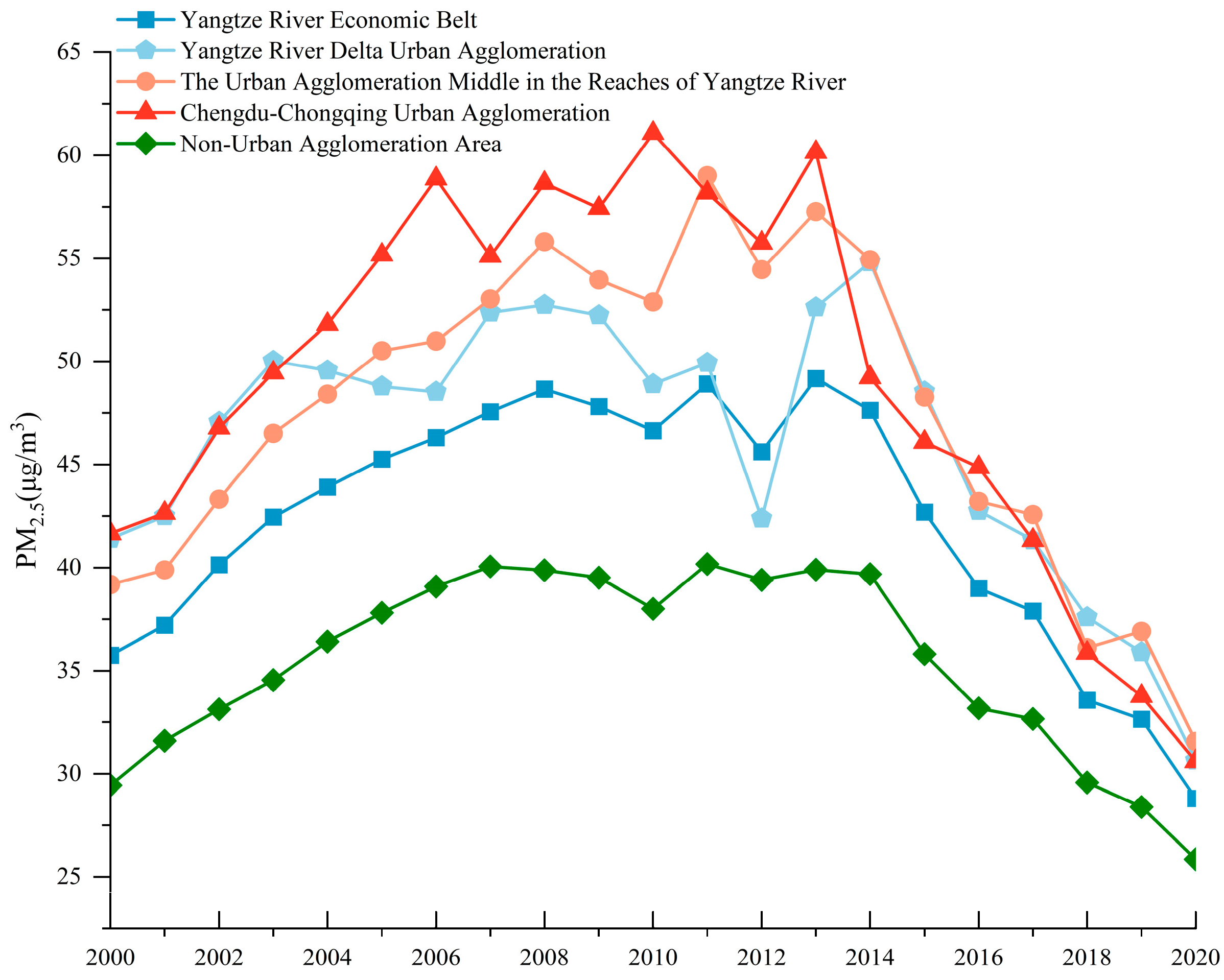
3.1.1. Time-Series Evolution

The concentration of PM2.5 in the YREB presents an “M”-shaped trend (Figure 6). The PM2.5 nuclear density curve basically showed a “big peak + small peak” situation during the study period, and the highest density value first shifted to the right and then to the left. The temporal evolution of PM2.5 concentrations from 2000 to 2020 can be classified into three distinct stages. Steady Rising Period (2000–2008). The concentration of PM2.5 area increased significantly, from 35.76 μg/m3 in 2000 to 48.67 μg/m3 in 2008, with an average annual increase of 1.614 μg/m3. This trend may be closely associated with the Chinese government’s proposal in 2002 to accelerate the improvement of the level of industrialization and urbanization. At this stage, energy consumption, especially coal consumption, in the study area increased rapidly, the scale of high-pollution industries such as the energy heavy chemical industry and petrochemical industry continued to expand, and the number of automobiles increased rapidly. Volatility Stabilization Period (2009–2013). At this stage, the concentration of PM2.5 in the YREB fluctuated between 46.65 μg/m3 and 49.18 μg/m3. The increasingly severe air pollution situation has affected China’s international image and the application and holding of major international events. To ensure the air quality during major events such as the 2010 Shanghai World Expo, the Chinese government implemented a collaborative mechanism for controlling air pollution, which led to a fluctuating pattern of decline or rise in the concentration of PM2.5. Rapid Decline Period (2014–2020). At this stage, the PM2.5 concentration rapidly decreases, from 47.64 μg/m3 in 2014 to 28.80 μg/m3 in 2020, with an average annual decrease of 3.14 μg/m3. The PM2.5 concentration in 2020 was 6.96 μg/m3 lower than that in 2000. The regional atmospheric pollution caused by PM2.5 pollutants poses severe risks to human health. In 2013, the Chinese government implemented an unprecedented “Air Pollution Prevention and Control Action Plan,” leading to a substantial decrease in PM2.5 concentrations during this period. These improvements indicate significant progress in addressing PM2.5 pollution in the YREB and enhancing air quality levels.
From 2000 to 2020, higher PM2.5 concentrations were observed in the three major urban agglomerations compared to non-urban agglomerations. Furthermore, significant variations in the changes of PM2.5 concentrations were observed among the three major urban agglomerations (Figure 7).
From 2000 to 2020, the average value of PM2.5 in the CCUA was 49.26 μg/m3, which was higher than the 47.56 μg/m3 of the YRMUA and 46.22 μg/m3 in the YRDUA. Through the comparison of the initial and final stages, the CCUA had the highest PM2.5 concentration in the early stage but decreased the most, followed by the YRDUA, and the YRMUA had the lowest initial but decreased the least. The average concentration of PM2.5 in the CCUA dropped from 41.66 μg/m3 in 2000 to 30.66 μg/m3 in 2020, a decrease of 11.06 μg/m3. The average concentration of PM2.5 in the YRDUA dropped from 41.40 in 2000 to 30.60 μg/m3 in 2020, a drop of 10.80 μg/m3. The average concentration of PM2.5 in the YRMUA dropped from 39.18 in 2000 to 31.57 μg/m3 in 2020, a decrease of 7.61 μg/m3.
From 2000 to 2020, PM2.5 concentrations exhibited significant fluctuations in the YRDUA. It displayed an upward trend from 2003 to 2014, followed by a rapid decline thereafter. The temporal variation of PM2.5 concentrations in the CCUA and the YRMUA mirrored that of the overall study area. From 2000 to 2004, both the CCUA and the YRDUA had significantly higher PM2.5 concentrations compared to the YRMUA. Between 2005 and 2013, PM2.5 concentrations in the CCUA and the YRMUA fluctuated and increased, surpassing that in the YRDUA. However, a rapid downward trend in PM2.5 concentrations was observed in all three major urban agglomerations after 2014.

3.1.2. Spatial Evolution Pattern

Spatially, the distribution of PM2.5 concentrations exhibit distinct patterns with higher levels in the eastern regions and lower levels in the western regions (Figure 8). Additionally, there is a noticeable trend of higher concentrations in the northern areas of the Yangtze River and lower concentrations in the southern regions. From an urban agglomeration standpoint, the central regions of the CCUA and the YRMUA primarily constitute areas with high levels of pollution, whereas the high-pollution agglomeration areas within the YRDUA are predominantly situated in the northern region. From 2005 to 2010, the CCUA exhibited relatively high PM2.5 concentrations, with Ziyang City and Neijiang City being the main areas of high pollution. Similarly, the YRDUA witnessed high PM2.5 pollution along both sides of the river. Notably, the northern part of the YRMUA was correlated with the high PM2.5 pollution area in the northern part of the YRDUA. By 2020, the concentration of PM2.5 in all three major urban agglomerations had decreased, resulting in significantly improved air quality compared to 2000. Regarding local changes, most cities south of the Yangtze River exhibit relatively stable pollution levels. The pollution status of most cities north of the Yangtze River fluctuates greatly, showing a trend of increasing first and then weakening. By 2020, the pollution status of most cities has been significantly improved. There are several possible reasons for the formation of this spatial distribution pattern. Firstly, the western cities of the YREB are located in the Yunnan-Guizhou Plateau, characterized by higher elevations, sparse population, lower levels of industrialization, and lower emissions of pollutants from human activities, resulting in lower PM2.5 concentrations. Secondly, the northern regions of the YREB are traditional heavy industrial bases in China, heavily reliant on coal as the primary energy source. Additionally, these areas experience harsh winter climates with poor conditions for pollutant dispersion, leading to higher PM2.5 concentrations. Thirdly, the Wuhan metropolitan area and the CCUA are undergoing rapid industrialization and urbanization processes, resulting in high emissions of air pollutants and severe air pollution, making them the most heavily polluted and concentrated areas in the YREB.

3.2. Spatial Correlation and Agglomeration Analysis

3.2.1. Global Moran’s I

From 2000 to 2020, the overall Moran’s I index for the YREB exceeded 0.5 and achieved statistical significance at the 1% level (Table 1). This signifies a notable positive spatial correlation in PM2.5 concentrations within the study area, indicating clear spatial agglomeration characteristics. Analyzing the time series, the global Moran’s I index in the YREB between 2000 and 2020 exhibited a trend of increasing fluctuations. This demonstrates the growing significance of the agglomeration effect. Consequently, changes in PM2.5 concentrations are significantly influenced by neighboring regions, with this influence intensifying over time.

3.2.2. Distribution Pattern of Cold-Hot Spot

Through the analysis of spatial cold-hot spot, the spatial clustering characteristics of PM2.5 concentrations in the YREB were explored. The significant hotspots of PM2.5 concentrations are predominantly located in the middle and lower reaches of the northern region of the Yangtze River, while the significant cold spots are concentrated in the southwestern part of the YREB (Figure 9). Significant cold-hot spot areas are contiguously distributed, and a few areas are scattered. Significant hotspots are concentrated in Hubei, Anhui, and northern Jiangsu provinces north of the Yangtze River. This may be due to the concentration of industries in northern Hubei, Anhui, and Jiangsu provinces, and the fact that several cities are transportation hubs, including Wuhan, Huangshi, Yichang, and Xiangyang in Hubei Province, Hefei, Huaibei, Huainan, and Tongling in Anhui Province, and Nanjing, Changzhou, and Nantong in Jiangsu Province. Additionally, the above-mentioned areas are characterized by relatively flat terrain and poor air circulation, resulting in a longer residence time for PM2.5.
Significant cold spots are primarily concentrated in western Sichuan Province and Yunnan Province. In terms of human factors, Yunnan Province has a low degree of industrialization, low traffic density, and low pollutant emissions from stationary and mobile sources. It can be observed that the significant hot spots of PM2.5 in the YREB have exhibited a gradual decline, whereas the significant cold spots have exhibited a persistent increase.

3.3. Analysis of Multi-Scale Driving Factors

3.3.1. Descriptive Statistics and Model Selection

To ensure data stability and to mitigate issues arising from heteroscedasticity and collinearity, this study performed standardization on variables with large values to reduce data analysis challenges caused by these factors (Table 2).
Before constructing the SPDM, it is essential to assess the need for spatial regression and evaluate the appropriateness of model selection. For example, Wei [48], showed that SPDM can degenerate into SPEM or SPLM.
According to the Elhorst [49] space testing theory and existing research, the model is determined in three steps. First, as presented in Table 3, both the LM statistic and the robust LM statistic rejected the null hypothesis at the 1% significance level, indicating the need to include spatial effects in the regression model. Secondly, the Likelihood Ratio estimation (LR) and Wald statistics were utilized to evaluate whether the SPDM could degenerate into SPEM or SPLM. Both LR and Wald statistics rejected the null hypothesis at the 1% significance level, demonstrating that SPDM cannot degenerate into SPEM or SPLM. Finally, in the selection of fixed effects and random effects, the Hausman test results indicated a p-value of 0, leading to the selection of fixed effects.
The ρ and the λ both show significant positive values, providing substantial evidence that spatial effects play a crucial role in studying the influencing factors of PM2.5 concentrations. This finding underscores the importance of considering spatial effects in the analysis (Table 4). For comparative experimental results, the Log-L of the SPDM was the highest, and its Adjust-R2 was significantly better than the other two. Therefore, the SPDM is the most suitable for this study.

3.3.2. Multi-Scale Impact Effect Analysis

The coefficient of ρ is 0.9240, and it passes the 1% significance level test, indicating that PM2.5 concentrations have a significant spatial positive spillover effect (Table 4). The decrease in PM2.5 concentrations in this city will have a significant impact on reducing the PM2.5 concentrations in other cities through geographical association. The positive spatial spillover effects of PM2.5 concentrations can be attributed to three main factors. Firstly, the competition effect. With the inclusion of environmental protection and ecological civilization in the performance assessment of government officials in China, seeking a green development path that combines economic growth with environmental protection has become one of the development goals for local governments at all levels [50]. Therefore, achieving environmental improvement goals such as reducing PM2.5 concentrations helps promote a healthy competition among local governments to become “demonstrators of environmental protection” in the context of green development. Secondly, the demonstration effect. Successful practices in PM2.5 concentration control in certain cities can have a demonstration and imitation effect on other regions through information exchange, the movement of officials, and technological spillovers. This facilitates the acceleration of transformation and catching-up in regions with higher PM2.5 concentrations by learning from and adopting these experiences and technologies. Thirdly, the economic linkage effect [51]. The reduction in PM2.5 concentrations in cities signifies a corresponding shift towards greener economic growth. The optimization and adjustment of economic growth patterns, driven by market mechanisms, can transmit through interregional industrial linkages to economically linked areas. This process facilitates the emergence of “green” new economic growth points in these areas, thereby driving the coordinated transformation of their economic growth patterns.
Among the human factors, the coefficients of economic development level and secondary industry proportion on PM2.5 concentrations are 0.4339 and 0.1727, respectively. At present, certain regions in the YREB prioritize economic development at the expense of the air environment. These regions, particularly areas along the Yangtze River, northern Jiangsu, and the northwestern Sichuan Basin, still have a significant presence of secondary industries, including large-scale petrochemicals, oil and gas chemicals, iron and steel, and equipment manufacturing, which are known for their pollution. These industries contribute to a substantial proportion of the industrial structure. The inefficient consumption of resources, such as coal and oil, by the secondary industry significantly contributes to the increase. The coefficients of population density and energy consumption on PM2.5 concentrations were 0.1461 and 0.0185, respectively. This result confirms the views of Malthusianism and Boslappism on the relationship between population and environment. Industrial sources and traffic sources are still the main sources of PM2.5 in the YREB. The rise in population density contributes to an increase in traffic exhaust and energy consumption, subsequently leading to higher PM2.5 concentrations. The influence coefficients of urban built-up area proportion, electricity consumption, and bus number on PM2.5 concentrations are −0.1171, −0.0569, −0.0200, respectively, and pass the significance test at 5%, 1%, and 1% levels, respectively. Urban expansion has resulted in the conversion of rural ecological land, leading to an increase in NDVI. Increased use of public transportation has decreased the use of private cars, reducing the generation of PM2.5 from this source of transportation. Furthermore, the increased proportion of clean energy sources has contributed to a reduction in the share of thermal power generation in the electricity sector.
In terms of natural factors (Table 4), annual average temperature (−0.0107, p = 1%), annual precipitation (−0.0661, p = 10%), annual average wind speed (−0.0201, p = 1%), and NDVI (−0.4586, p = 1%) have significantly negative influence coefficients on PM2.5 concentrations, while annual average relative humidity (0.8944, p = 1%) has a significant positive influence coefficient on PM2.5 concentrations. These findings indicate that increases in annual average temperature, annual precipitation, annual average wind speed, and NDVI are associated with a reduction in PM2.5 concentrations. Conversely, an increase in annual average relative humidity is conducive to an increase in PM2.5 concentrations. The inhibitory effect of mean annual temperature on PM2.5 provides an explanation for the seasonal variation of PM2.5 concentrations in the YREB. The YREB has more rainfall. Precipitation plays a dual role in relation to PM2.5 concentrations. It serves as a cleansing mechanism by removing PM2.5 particles from the air. Additionally, precipitation triggers chemical reactions that facilitate the deposition of certain PM2.5 particles, leading to a decrease in their concentration in the air. Conversely, higher relative humidity promotes the formation of PM2.5. Increased wind speed enhances the settling velocity of PM2.5 particles, thereby reducing their concentration in the air. Regions characterized by high vegetation coverage typically experience slower industrialization and urbanization processes. Consequently, these areas exhibit relatively low emissions of air pollutants. Moreover, the presence of abundant vegetation has a certain absorption effect on PM2.5, further reducing its concentration in the air.
Further analysis was conducted to examine the heterogeneity within the three major urban agglomerations. In terms of human factors, the proportion of secondary industry (0.6448) and population density (0.2580) emerged as the primary contributors to PM2.5 pollution in the CCUA. Meanwhile, population density (0.0609) and energy consumption (0.0386) were identified as significant factors influencing the increase in PM2.5 concentrations in the YRMUA. In the YRDUA, the dominant factors were the secondary industry (0.6893) and the urban built-up area (0.2297). From the PM2.5 control perspective, the proportion of urban built-up area reduces PM2.5 concentrations in both the CCUA (−0.9636) and the YRMUA (−0.1652). In the YRDUA, power consumption (−0.0881) emerged as the primary human factor for PM2.5 pollution control. Regarding natural factors, their impact on PM2.5 concentrations was most significant and extensive in the YRDUA, followed by the YRMUA, while the CCUA exhibited the least impact. In the YRDUA, five natural factors exhibited a significant influence, while the YRMUA was affected by four, and the CCUA by only two (Table 5). Among these factors, NDVI played a prominent role in reducing PM2.5 concentrations in both the YRMUA and the YRDUA. However, in the CCUA, NDVI was found to promote PM2.5 concentrations. Additionally, annual average relative humidity proved beneficial for PM2.5 control in the YRDUA (−0.9084), while it exacerbated PM2.5 concentrations in the CCUA.
In the CCUA, the primary factors are the proportion of secondary industry (0.6448) and population density (0.2580). In the YRMUA, population density (0.0609) and energy consumption (0.0386) play significant roles in the increase of PM2.5 concentration. Meanwhile, the dominant factors in the YRDUA are the proportion of secondary industry (0.6893) and the proportion of urban built-up area (0.2297). Regarding PM2.5 control, the proportion of urban built-up area is the main factor for the decline of PM2.5 concentrations in both the CCUA (−0.9636) and the YRMUA (−0.1652). In the YRDUA, power consumption (−0.0881) emerges as the dominant human factor for PM2.5 pollution control. Among natural factors, NDVI stands out as one of the primary contributors to the reduction of PM2.5 concentrations in both the YRMUA and the YRDUA, while in the CCUA, it promotes an increase in PM2.5 concentrations. The increase in annual average relative humidity is beneficial to the governance of PM2.5 in the YRDUA (−0.9084), but it aggravates the concentrations of PM2.5 in the YRMUA (0.6073). NDVI, the proportion of the secondary industry, and the proportion of urban built-up area collectively influence the changes in PM2.5 concentrations across the three major urban agglomerations. Additionally, population density raises PM2.5 concentrations in the CCUA. Notably, the annual average relative humidity emerges as a leading factor affecting PM2.5 concentrations in both the YRMUA and the YRDUA, albeit with contrasting effects.
Through SPDM regression analysis, this study provides an initial understanding of the influence of natural and human factors. However, it is important to note that the coefficients obtained from the SPDM regression do not represent the marginal effects of explanatory variables or provide a comprehensive assessment of the total effect [47]. Therefore, this paper employs the partial differential method to decompose the W*X regression results of SPDM into local effects, spillover effects, and total effects, allowing for a more thorough examination of the factors influencing PM2.5 concentrations.

3.3.3. Decomposition of Multi-Scale Effects Based on P.D.E.

The local and spillover effects of the proportion of the secondary industry, the number of buses, and the energy consumption on PM2.5 concentrations are all significantly negative (Table 6). Conversely, both the local and spillover effects of the urban built-up area proportion and population density on PM2.5 concentrations are significantly positive. Among the human factors, the proportion of the secondary industry, the proportion of the urban built-up area, and the population density are the primary drivers of PM2.5 changes in the YREB. Regarding natural factors, annual precipitation and NDVI emerge as the two dominant factors influencing PM2.5 concentrations in the region. Specifically, the local and spillover effects of annual precipitation on PM2.5 concentrations were −0.1709 and −9.0718, respectively. This indicates that increased annual precipitation has a substantial negative impact on the reduction of PM2.5 concentrations in the region and adjacent areas, ultimately leading to an inhibitory effect on PM2.5 concentrations across the entire region. Additionally, the annual mean relative humidity and NDVI significantly influence PM2.5 concentrations in opposite locations (Table 6). The local effect of annual average relative humidity promotes an increase in PM2.5 concentrations, while the local effect of NDVI promotes a decrease in PM2.5 concentrations. Furthermore, the spillover effects of each dominant factor outweigh the local effects. This spatial perspective demonstrates that the primary factors primarily influence PM2.5 concentrations through spillover effects.
The results of the total effect (Table 7) reveal that among the natural factors, the primary factors in the CCUA are the annual average relative humidity and NDVI. In the YRMUA and YRDUA, the main natural factors are the annual average temperature and annual average wind speed. Additionally, annual precipitation also emerges as a dominant natural factor in the YRDUA.
Significant variations exist in the dominant natural factors driving changes in PM2.5 concentrations among the CCUA and the other two major urban agglomerations. The YRDUA experiences the widest range of influences from natural factors on PM2.5 concentrations. Regarding human factors (Table 7), population density and power consumption emerge as the dominant factors in the CCUA. Economic development level and power consumption play crucial roles for PM2.5 concentrations in the YRDUA. The dominant factors in the YRMUA include the proportion of urban built-up area, population density, number of buses, and energy consumption. Considerable disparities exist in the human-driven factors contributing to changes in PM2.5 concentrations among the three major urban agglomerations, with the YRMUA being the most significantly influenced by human factors.

4. Discussion

4.1. Effects of Natural Factors and Human Factors on PM2.5 Concentrations

Previous studies have demonstrated that regional PM2.5 concentrations are influenced by both natural factors and human factors, specifically socioeconomic factors [29,30,39,42]. Our research supports this point of view. From a basin-scale perspective, both natural factors and human factors have played a significant role in driving the variations of PM2.5 concentrations in the YREB. This is mainly because PM2.5 in the YREB comes from both nature and human activities. However, the primary source of PM2.5 is anthropogenic emissions, which are primarily generated from human activities such as industrial production, transportation, construction, and agricultural practices. Based on the SPDM, we found that the annual average relative humidity and NVDI are the natural dominant factors. The economic development level, the proportion of secondary industry and urban built-up area, and population density are the human-driven factors. Compared with existing studies [4,20,52], this study analysis of the factors influencing PM2.5 considers both natural and human factors. Additionally, it identifies the dominant and non-dominant factors. The research findings offer practical data support for the YREB in adopting a PM2.5 control strategy that primarily focuses on regulating human activities while also complementing efforts to improve the ecological environment. The correlation between economic development and PM2.5 concentrations substantiates the “EKC” hypothesis [47]; that is, economic growth leads to serious and extensive environmental degradation under the traditional development paradigm. The share of the secondary industry’s output value plays a crucial role in promoting PM2.5 concentrations in the YREB. This is due to the adoption of a traditional industrialization model in the YREB, characterized by the approach of “pollution first, governance later.” This model has led to an increase in PM2.5 concentrations through industrial emissions, coal burning, construction, transportation, and other production activities. The impact of population density on PM2.5 concentrations supports the conclusions of Malthusism and Boslapism [47]. Compared with other studies on urbanization and PM2.5 [35,40], this study found that urban expansion can reduce PM2.5 concentrations in the YREB. This may be because, under the background of the United Nations’ Sustainable Development Goals, urban expansion has led to the relocation of certain industrial activities, such as polluting enterprises, from city centers to peri-urban areas, resulting in a reduction in PM2.5 concentrations [53]. Additionally, from 2014 to 2019, the total area of urban green spaces in China increased from 1.82 million hectares to 2.285 million hectares, and the improved urban greening ratio has effectively decreased PM2.5 concentrations. Furthermore, the expansion of urban construction land has attracted more rural populations to migrate from rural to urban areas [54]. This has further resulted in an increase in rural ecological land and NDVI (Normalized Difference Vegetation Index), thus reducing PM2.5 concentrations through plant uptake. This result is similar to the findings of Zhang [55], who found that urban expansion and rural depopulation can bring large transient carbon sinks. An increase in the annual average relative humidity is conducive to the generation of PM2.5, but with the increase of humidity, the probability of precipitation also increases, and the scouring effect will cause the precipitation of fine particles. To sum up, this study found that reducing PM2.5 concentrations requires a combination of natural and human factors, and formulating comprehensive measures from multiple perspectives, rather than just considering a single factor.
In the context of urban agglomerations, both natural and human factors influence PM2.5 concentrations in the YRDUA and the YRMUA. However, PM2.5 concentrations in the CCUA are primarily influenced by human factors. The YRDUA is located near the coastline, and is affected by ocean air currents, topography, and complex urbanization processes, resulting in PM2.5 concentrations being restricted by many factors both natural and artificial. The climatic conditions of the YRMUA are relatively different (the natural conditions are relatively stable but the internal differences are large), and in different seasons, natural and human factors have different effects on PM2.5 concentrations. The CCUA experiences a relatively stable interannual variation of natural factors due to its unique geographical location and climatic conditions. Chengdu-Chongqing, on the other hand, has implemented various measures to control industrial emissions and vehicle exhaust emissions. As a result, PM2.5 concentrations in this region are more influenced by human factors. The NDVI, the proportion of the output value of the secondary industry, and the proportion of the urban built-up area are identified as common influential factors for PM2.5 variations in all three urban agglomerations. However, the specific locations where these factors have the most significant effects differ among the agglomerations. Urban expansion and rural population reduction in CCUA have released a large amount of ecological land, leading to the rise of NDVI, which may further absorb and purify some pollutants in the air. Nevertheless, in the case of the CCUA, the rapid process of industrialization and urbanization has led to an increase in PM2.5 concentrations that surpasses the potential purification effects of vegetation. As a result, the rise in NDVI alone may not be sufficient to counterbalance the increase in PM2.5 concentrations. In contrast, in the YRMUA, both NDVI, the proportion of the output value of the secondary industry, and the proportion of the urban built-up area exert significant inhibitory effects on PM2.5 concentrations. This is mainly because the YRMUA has undertaken part of the industrial transfer of the YRDUA, and its secondary industry has received new technology and equipment, which can reduce pollutant emissions. For the YRDUA, its level of urbanization, advanced industrial structure, and population density are relatively high. The development of the secondary industry is associated with an increase in pollutant emissions originating from industrial sources, transportation sources, residential sources, and other sources. This study provides a practical value, namely, the governance of PM2.5 in the YREB should not only promote trans-regional joint governance from the overall consideration, but also formulate differentiated governance strategies from the perspective of urban agglomeration.

4.2. Local Effects and Spillover Effects

The local effect of annual average relative humidity on PM2.5 concentrations is significantly positive, and the spillover effect is not significant. Since it is difficult for moisture to diffuse in the air, the humidification effect will only affect local areas with relatively high relative humidity, and it is difficult to produce spatial spillover effects. The local impact of NDVI on PM2.5 concentrations exhibited a significant negative relationship, while the spillover effect was found to be insignificant. This may be because the spatial distribution characteristics of NDVI changes are usually related to vegetation distribution, and its impact range is relatively small. The local effect and spillover effect of annual precipitation on PM2.5 concentrations are significantly negative. Precipitation plays a dual role in reducing air particulate matter.
The local effect and spillover effect of annual precipitation on PM2.5 concentrations demonstrates a significant negative relationship. Precipitation not only contributes to reducing air particulate matter locally through its cleaning effect, but also produces spatial spillover effect through transport and diffusion. Similarly, both the local benefit and spillover effect of the output value of the secondary industry on PM2.5 exhibit a significant negative relationship. These effects are determined through the decomposition of the W*X coefficients into local and spillover components. As far as the location is concerned, the secondary industry brought about by industrial transfer is often higher end than the other forms of secondary industry in the region. The former, referring to areas with less environmental pollution resulting from industrial upgrading, has successfully reduced PM2.5 concentrations. Among them, the partial differential estimation results of the proportion of urban built-up areas are opposite to the previous regression results. This is because urban expansion will not only release a large amount of ecological land, but also increase PM2.5 emissions through infrastructure and housing construction. At the same time, urbanization will lead to synergistic growth of PM2.5 in neighboring regions through cross-regional population flow and interconnection of industrial production.
In the CCUA, the dominant factors influencing the local effect include the proportion of urban built-up area, population density, power consumption, and NDVI. The dominant factors contributing to the spillover benefits are population density, power consumption, NDVI, and annual average relative humidity. In the YRMUA, the local effect factors include the proportion of urban built-up area, population density, power consumption, and NDVI. Additionally, the dominant factors contributing to the spillover effects are primarily the proportion of urban built-up area, population density, annual average temperature, and relative humidity. The local effect factors in the YRDUA are the proportion of urban built-up area, power consumption, annual average relative humidity, and NDVI, and the main factors of spillover effects are economic development level, power consumption, annual precipitation, and annual average temperature.
Affected by ocean air currents, the YRDUA is more likely to form rainfall when the annual average relative humidity is high, thus reducing PM2.5 concentrations. However, the YRMUA is far away from the coast, and the increase in annual average humidity will cause water molecules in the air to adsorb pollutants. In the case of the CCUA, characterized by better ecological conditions, the increase in NDVI value may result in a vegetation purification effect that is smaller compared to the growth rate of PM2.5 emissions. However, for the YRMUA and the YRDUA with relatively poor ecological status, the increase in NDVI value will accelerate the purification rate of PM2.5 by vegetation and reduce their PM2.5 concentrations. In the relatively underdeveloped CCUA and the YRMUA, urban expansion has released a large amount of ecological land. The urban expansion of the YRDUA promotes internal coordinated development, which leads to concentrated pollution. The spillover effects of both natural and human factors primarily occur through processes such as air transport, sedimentation, and complex chemical reactions. In the case of the YRDUA, characterized by a flat terrain and coastal location, various factors exhibit significant spatial spillover effects. Conversely, the CCUA, situated in an inland area dominated by basins, does not show distinct spatial spillover effects for various factors.

4.3. Policy Suggestion

Our research has revealed a significant spatial correlation and evident spatial agglomeration characteristics in the concentration of PM2.5 within the study area. This indicates that efforts to control air pollution in the YREB should prioritize the actual requirements for protecting and restoring the ecological environment and carry out coordinated governance of the ecological environment from multiple dimensions. Collaborative governance of the ecological environment can adjust the conflicts of different stakeholders, and more effectively adapt to and solve the complexity and uncertainty of the system. To enhance the protection and restoration of the ecological environment, it is imperative to move beyond the limitations of the government’s single-subject governance model and establish a collaborative governance mechanism led by the government, involving multiple stakeholders. This entails promoting collaboration at the national and local levels, fostering cooperation among local governments, government departments, enterprises, and the public.
It is essential to propose corresponding measures and recommendations based on the dominant factors influencing PM2.5 concentration. Firstly, the government should establish and refine phased mid- and long-term improvement targets aligned with air pollution control objectives. This should involve strengthening the structural adjustments in the secondary and tertiary industries and implementing source control measures for power generation and energy consumption. Secondly, the YREB should carefully consider the relationship between urban land use and ecological land use, aiming to enhance the efficiency of urban land utilization while expanding the areas dedicated to ecological land use. Lastly, it is crucial to account for the variations in driving factors influencing PM2.5 concentrations among different urban agglomerations. Adopting standardized control measures without considering these differences could prove to be ineffective. The YRDUA needs to implement differentiated global PM2.5 pollution controls along the river and the coast, focusing on Ningbo, Zhoushan, Shanghai, Suzhou, Nantong, Lianyungang, Yancheng, and other cities. Midstream urban agglomerations need to pay attention to the PM2.5 emission pressure brought about by the common development of both traditional industries and emerging industries, implement industrial control and coordinated control of compound pollutants and emission reduction control, and implement high-standard industry access requirements. Focus on Jingzhou, Jingmen, Xiangyang, Yichang, Wuhan, and other cities on the Hanjiang Plain in Hubei, the Changsha-Zhuzhou-Tan town group in Hunan, and the Xinyiping town group in Jiangxi and other contiguous areas. The CCUA needs to strengthen industrial PM2.5 pollution control at the source from the perspective of industry access and technical equipment level improvement and promote the overall improvement of pollution prevention and control technology.

4.4. Limitations and Future Research Directions

This study has certain limitations. Firstly, the scale of analysis plays a crucial role in the calculation of PM2.5 concentrations. This study focused on cities as the basic unit to explore the spatiotemporal characteristics and influencing factors of PM2.5 concentrations. However, at the county or grid scale, the influencing factors of PM2.5 concentrations may vary. In future research, we intend to investigate the distribution patterns and influencing factors of PM2.5 at more refined scales. Secondly, the mechanism underlying the interaction of natural and anthropogenic factors on PM2.5 concentrations is complex. Therefore, our future focus will be on exploring this mechanism in depth. Lastly, the spillover pathways of PM2.5 governance are crucial for regional collaborative governance, and this is one of the directions we intend to explore in the future.

5. Conclusions

In this study, combined with remote sensing interpretation data and statistical data, using GIS analysis methods and spatial econometric models, this study explored the multi-scale driving effect of PM2.5 in the YREB under the joint action of natural and human factors. Draw the following main conclusions.
  • From 2000 to 2020, PM2.5 concentrations in the YREB exhibited an “M”-shaped trend.
  • The spatial distribution of PM2.5 concentrations shows distinct characteristics, with higher concentrations observed in the eastern regions and lower concentrations in the western regions. Moreover, the northern areas of the Yangtze River tend to have higher PM2.5 concentrations compared to the southern areas. In terms of urban agglomerations, the central areas of the CCUA and the YRMUA are predominantly characterized by high-pollution concentrations, while the high-pollution agglomeration areas in the YRDUA are primarily located in the northern region.
  • From a regional perspective, concentrations of PM2.5 in the YREB are significantly influenced by both natural and human factors. The key factors contributing to the local effect on PM2.5 concentrations in the YREB include the level of economic development, the proportion of urban built-up area, population density, annual average relative humidity, and NDVI. The main factors driving the spillover effect are the proportion of output value of the secondary industry, the proportion of urban built-up area, population density, and annual precipitation.
  • In terms of urban agglomerations, changes in PM2.5 concentrations in the three major urban agglomerations, namely the CCUA, the YRMUA and the YRDUA, are influenced by NDVI, the proportion of secondary industries, and the proportion of urban built-up areas. Additionally, in the CCUA, population density also plays a significant role in driving changes in PM2.5 concentrations. Furthermore, the annual average relative humidity is a leading factor for changes in PM2.5 concentrations in both the YRMUA and the YRDUA, but its impact direction differs between the two regions.

Supplementary Materials

The following supporting information can be downloaded at: https://www.mdpi.com/article/10.3390/rs15133356/s1, Figure S1: Evolution characteristics of the spatial pattern of TEM in the YREB from 2006 to 2020; Figure S2: Evolution characteristics of the spatial pattern of HUM in the YREB from 2006 to 2020; Figure S3: Evolution characteristics of the spatial pattern of PRE in the YREB from 2006 to 2020; Figure S4: Evolution characteristics of the spatial pattern of WIN in the YREB from 2006 to 2020; Figure S5: Evolution characteristics of the spatial pattern of NDVI in the YREB from 2006 to 2020; Figure S6: Evolution characteristics of the spatial pattern of PGDP in the YREB from 2006 to 2020; Figure S7: Evolution characteristics of the spatial pattern of SEC in the YREB from 2006 to 2020; Figure S8: Evolution characteristics of the spatial pattern of BUI in the YREB from 2006 to 2020; Figure S9: Evolution characteristics of the spatial pattern of POPD in the YREB from 2006 to 2020; Figure S10: Evolution characteristics of the spatial pattern of ELE in the YREB from 2006 to 2020; Figure S11: Evolution characteristics of the spatial pattern of CAR in the YREB from 2006 to 2020; Figure S12: Evolution characteristics of the spatial pattern of ENE in the YREB from 2006 to 2020.

Author Contributions

Writing the original draft, S.L.; Review and editing, G.W. and Y.L.; Investigation, L.B.; Methodology, G.W. and Y.L. All authors have read and agreed to the published version of the manuscript.

Funding

This study was sponsored by the National Natural Science Foundation of China (Grant No. 42271209) and Project of Jiangxi Provincial Humanities and Social Science (Grant No. JJ21201).

Data Availability Statement

If need data from this article, please contact the corresponding author.

Conflicts of Interest

The authors declare that they have no competing interest.

References

  1. Sicard, P.; Agathokleous, E.; Anenberg, S.C.; De Marco, A.; Paoletti, E.; Calatayud, V. Trends in urban air pollution over the last two decades: A global perspective. Sci. Total Environ. 2023, 858, 13. [Google Scholar] [CrossRef] [PubMed]
  2. Jbaily, A.; Zhou, X.D.; Liu, J.; Lee, T.H.; Kamareddine, L.; Verguet, S.; Dominici, F. Air pollution exposure disparities across US population and income groups. Nature 2022, 601, 228–233. [Google Scholar] [CrossRef] [PubMed]
  3. Fuller, R.; Landrigan, P.J.; Balakrishnan, K.; Bathan, G.; Bose-O’Reilly, S.; Brauer, M.; Caravanos, J.; Chiles, T.; Cohen, A.; Corra, L.; et al. Pollution and health: A progress update. Lancet Planet. Health 2022, 6, E535–E547. [Google Scholar] [CrossRef] [PubMed]
  4. Apte, J.S.; Marshall, J.D.; Cohen, A.J.; Brauer, M. Addressing Global Mortality from Ambient PM2.5. Environ. Sci. Technol. 2015, 49, 8057–8066. [Google Scholar] [CrossRef] [PubMed]
  5. Liu, J.; Han, Y.Q.; Tang, X.; Zhu, J.; Zhu, T. Estimating adult mortality attributable to PM2.5 exposure in China with assimilated PM2.5 concentrations based on a ground monitoring network. Sci. Total Environ. 2016, 568, 1253–1262. [Google Scholar] [CrossRef]
  6. Geng, G.N.; Zheng, Y.X.; Zhang, Q.; Xue, T.; Zhao, H.Y.; Tong, D.; Zheng, B.; Li, M.; Liu, F.; Hong, C.P.; et al. Drivers of PM2.5 air pollution deaths in China 2002–2017. Nat. Geosci. 2021, 14, 645–650. [Google Scholar] [CrossRef]
  7. Ji, X.; Yao, Y.X.; Long, X.L. What causes PM2.5 pollution? Cross-economy empirical analysis from socioeconomic perspective. Energy Policy 2018, 119, 458–472. [Google Scholar] [CrossRef]
  8. Li, S.; Liu, Y.; Elahi, E.; Meng, X.; Deng, W. A new type of urbanization policy and transition of low-carbon society: A “local- neighborhood” perspective. Land Use Policy 2023, 131, 106709. [Google Scholar] [CrossRef]
  9. Yang, T.; Zhou, K.L.; Ding, T. Air pollution impacts on public health: Evidence from 110 cities in Yangtze River Economic Belt of China. Sci. Total Environ. 2022, 851, 8. [Google Scholar] [CrossRef]
  10. Zhang, R.; Jing, J.; Tao, J.; Hsu, S.C.; Wang, G.; Cao, J.; Lee, C.S.L.; Zhu, L.; Chen, Z.; Zhao, Y.; et al. Chemical characterization and source apportionment of PM2.5 in Beijing: Seasonal perspective. Atmos. Chem. Phys. 2013, 13, 7053–7074. [Google Scholar] [CrossRef] [Green Version]
  11. Dong, Z.X.; Xing, J.; Zhang, F.F.; Wang, S.X.; Ding, D.; Wang, H.L.; Huang, C.; Zheng, H.T.; Jiang, Y.Q.; Hao, J.M. Synergetic PM2.5 and O-3 control strategy for the Yangtze River Delta, China. J. Environ. Sci. 2023, 123, 281–291. [Google Scholar] [CrossRef]
  12. Colmer, J.; Hardman, I.; Shimshack, J.; Voorheis, J. Disparities in PM2.5 air pollution in the United States. Science 2020, 369, 575–578. [Google Scholar] [CrossRef]
  13. Wang, S.J.; Zhou, C.S.; Wang, Z.B.; Feng, K.S.; Hubacek, K. The characteristics and drivers of fine particulate matter (PM2.5) distribution in China. J. Clean Prod. 2017, 142, 1800–1809. [Google Scholar] [CrossRef]
  14. Ming, L.L.; Jin, L.; Li, J.; Fu, P.Q.; Yang, W.Y.; Liu, D.; Zhang, G.; Wang, Z.F.; Li, X.D. PM2.5 in the Yangtze River Delta, China: Chemical compositions, seasonal variations, and regional pollution events. Environ. Pollut. 2017, 223, 200–212. [Google Scholar] [CrossRef]
  15. Zhou, C.S.; Chen, J.; Wang, S.J. Examining the effects of socioeconomic development on fine particulate matter (PM2.5) in China’s cities using spatial regression and the geographical detector technique. Sci. Total Environ. 2018, 619, 436–445. [Google Scholar] [CrossRef]
  16. Zhang, D.H.; Zhou, C.S.; He, B.J. Spatial and temporal heterogeneity of urban land area and PM2.5 concentration in China. Urban Clim. 2022, 45, 15. [Google Scholar] [CrossRef]
  17. He, Q.Q.; Huang, B. Satellite-based mapping of daily high-resolution ground PM2.5 in China via space-time regression modeling. Remote Sens. Environ. 2018, 206, 72–83. [Google Scholar] [CrossRef]
  18. Cheng, Z.; Luo, L.; Wang, S.X.; Wang, Y.G.; Sharma, S.; Shimadera, H.; Wang, X.L.; Bressi, M.; de Miranda, R.M.; Jiang, J.K.; et al. Status and characteristics of ambient PM2.5 pollution in global megacities. Environ. Int. 2016, 89–90, 212–221. [Google Scholar] [CrossRef]
  19. Zhang, Q.; Zheng, Y.X.; Tong, D.; Shao, M.; Wang, S.X.; Zhang, Y.H.; Xu, X.D.; Wang, J.N.; He, H.; Liu, W.Q.; et al. Drivers of improved PM2.5 air quality in China from 2013 to 2017. Proc. Natl. Acad. Sci. USA 2019, 116, 24463–24469. [Google Scholar] [CrossRef] [Green Version]
  20. Chen, Z.Y.; Chen, D.L.; Zhao, C.F.; Kwan, M.P.; Cai, J.; Zhuang, Y.; Zhao, B.; Wang, X.Y.; Chen, B.; Yang, J.; et al. Influence of meteorological conditions on PM2.5 concentrations across China: A review of methodology and mechanism. Environ. Int. 2020, 139, 21. [Google Scholar] [CrossRef]
  21. Guan, D.B.; Su, X.; Zhang, Q.; Peters, G.P.; Liu, Z.; Lei, Y.; He, K.B. The socioeconomic drivers of China’s primary PM2.5 emissions. Environ. Res. Lett. 2014, 9, 9. [Google Scholar] [CrossRef] [Green Version]
  22. Zhang, Y.; Shuai, C.Y.; Bian, J.; Chen, X.; Wu, Y.; Shen, L.Y. Socioeconomic factors of PM2.5 concentrations in 152 Chinese cities: Decomposition analysis using LMDI. J. Clean Prod. 2019, 218, 96–107. [Google Scholar] [CrossRef]
  23. Chen, G.B.; Li, S.S.; Knibbs, L.D.; Hamm, N.A.S.; Cao, W.; Li, T.T.; Guo, J.P.; Ren, H.Y.; Abramson, M.J.; Guo, Y.M. A machine learning method to estimate PM2.5 concentrations across China with remote sensing, meteorological and land use information. Sci. Total Environ. 2018, 636, 52–60. [Google Scholar] [CrossRef] [PubMed]
  24. Cheng, Z.H.; Li, L.S.; Liu, J. Identifying the spatial effects and driving factors of urban PM2.5 pollution in China. Ecol. Indic. 2017, 82, 61–75. [Google Scholar] [CrossRef]
  25. Zhao, R.; Zhan, L.P.; Yao, M.X.; Yang, L.C. A geographically weighted regression model augmented by Geodetector analysis and principal component analysis for the spatial distribution of PM2.5. Sustain. Cities Soc. 2020, 56, 9. [Google Scholar] [CrossRef]
  26. Li, G.Q.; Li, L.Y.; Liu, D.; Qin, J.H.; Zhu, H.J. Effect of PM2.5 pollution on perinatal mortality in China. Sci. Rep. 2021, 11, 12. [Google Scholar] [CrossRef]
  27. Li, X.Y.; Xue, W.H.; Wang, K.; Che, Y.F.; Wei, J. Environmental regulation and synergistic effects of PM2.5 control in China. J. Clean Prod. 2022, 337, 11. [Google Scholar] [CrossRef]
  28. Yang, F.Y.; Xu, Q.S.; Li, K.M.; Yuen, K.F.; Shi, W.M. The inhibition effect of bank credits on PM2.5 concentrations: Spatial evidence from high-polluting firms in China. Environ. Pollut. 2022, 308, 10. [Google Scholar] [CrossRef]
  29. Wang, Y.C.; Liu, C.G.; Wang, Q.Y.; Qin, Q.D.; Ren, H.H.; Cao, J.J. Impacts of natural and socioeconomic factors on PM2.5 from 2014 to 2017. J. Environ. Manage. 2021, 284, 9. [Google Scholar] [CrossRef]
  30. Chen, H.S.; Lin, Y.C.; Chiueh, P.T. Nexus of ecosystem service-human health-natural resources: The nature-based solutions for urban PM2.5 pollution. Sustain. Cities Soc. 2023, 91, 11. [Google Scholar] [CrossRef]
  31. Jin, Y.H.; Zhang, H.; Shi, H.; Wang, H.L.; Wei, Z.F.; Han, Y.X.; Cong, P.T. Assessing Spatial Heterogeneity of Factor Interactions on PM2.5 Concentrations in Chinese Cities. Remote Sens. 2021, 13, 5079. [Google Scholar] [CrossRef]
  32. Xia, S.Y.; Liu, X.J.; Liu, Q.; Zhou, Y.N.; Yang, Y. Heterogeneity and the determinants of PM2.5 in the Yangtze River Economic Belt. Sci. Rep. 2022, 12, 11. [Google Scholar] [CrossRef]
  33. Geng, G.N.; Xiao, Q.Y.; Liu, S.G.; Liu, X.D.; Cheng, J.; Zheng, Y.X.; Xue, T.; Tong, D.; Zheng, B.; Peng, Y.R.; et al. Tracking Air Pollution in China: Near Real-Time PM2.5 Retrievals from Multisource Data Fusion. Environ. Sci. Technol. 2021, 55, 12106–12115. [Google Scholar] [CrossRef]
  34. Yue, H.B.; He, C.Y.; Huang, Q.X.; Yin, D.; Bryan, B.A. Stronger policy required to substantially reduce deaths from PM2.5 pollution in China. Nat. Commun. 2020, 11, 10. [Google Scholar] [CrossRef] [Green Version]
  35. Shen, H.Z.; Tao, S.; Chen, Y.L.; Ciais, P.; Guneralp, B.; Ru, M.Y.; Zhong, Q.R.; Yun, X.; Zhu, X.; Huang, T.B.; et al. Urbanization-induced population migration has reduced ambient PM2.5 concentrations in China. Sci. Adv. 2017, 3, 13. [Google Scholar] [CrossRef] [Green Version]
  36. Hao, Y.; Peng, H.; Temulun, T.; Liu, L.Q.; Mao, J.; Lu, Z.N.; Chen, H. How harmful is air pollution to economic development? New evidence from PM2.5 concentrations of Chinese cities. J. Clean Prod. 2018, 172, 743–757. [Google Scholar] [CrossRef]
  37. Lin, H.; Wang, X.Y.; Bao, G.; Xiao, H.J. Heterogeneous Spatial Effects of FDI on CO2 Emissions in China. Earth Future 2022, 10, 23. [Google Scholar] [CrossRef]
  38. Zhai, S.X.; Jacob, D.J.; Wang, X.; Shen, L.; Li, K.; Zhang, Y.Z.; Gui, K.; Zhao, T.L.; Liao, H. Fine particulate matter (PM2.5) trends in China, 2013-2018: Separating contributions from anthropogenic emissions and meteorology. Atmos. Chem. Phys. 2019, 19, 11031–11041. [Google Scholar] [CrossRef] [Green Version]
  39. Bai, L.; Jiang, L.; Yang, D.Y.; Liu, Y.B. Quantifying the spatial heterogeneity influences of natural and socioeconomic factors and their interactions on air pollution using the geographical detector method: A case study of the Yangtze River Economic Belt, China. J. Clean Prod. 2019, 232, 692–704. [Google Scholar] [CrossRef]
  40. Zhu, W.W.; Wang, M.C.; Zhang, B.B. The effects of urbanization on PM2.5 concentrations in China’s Yangtze River Economic Belt: New evidence from spatial econometric analysis. J. Clean Prod. 2019, 239, 11. [Google Scholar] [CrossRef]
  41. Liu, P.X.; Zhong, F.L.; Yang, C.L.; Jiang, D.W.; Luo, X.J.; Song, X.Y.; Guo, J. Influence mechanism of urban polycentric spatial structure on PM2.5 emissions in the Yangtze River Economic Belt, China. J. Clean Prod. 2022, 365, 12. [Google Scholar] [CrossRef]
  42. Liu, X.J.; Xia, S.Y.; Yang, Y.; Wu, J.F.; Zhou, Y.N.; Ren, Y.W. Spatiotemporal dynamics and impacts of socioeconomic and natural conditions on PM2.5 in the Yangtze River Economic Belt. Environ. Pollut. 2020, 263, 9. [Google Scholar] [CrossRef] [PubMed]
  43. Kong, Y.; He, W.J.; Yuan, L.; Zhang, Z.F.; Gao, X.; Zhao, Y.E.; Degefu, D.M. Decoupling economic growth from water consumption in the Yangtze River Economic Belt, China. Ecol. Indic. 2021, 123, 9. [Google Scholar] [CrossRef]
  44. Mao, X.L.; Wang, L.C.; Pan, X.; Zhang, M.; Wu, X.J.; Zhang, W. A study on the dynamic spatial spillover effect of urban form on PM2.5 concentration at county scale in China. Atmos. Res. 2022, 269, 15. [Google Scholar] [CrossRef]
  45. Wang, K.F.; Liu, Y.; Wang, S.C.; Li, C.P. The spatial spillover effect of higher SO2 emission tax rates on PM2.5 concentration in China. Sci. Rep. 2023, 13, 13. [Google Scholar] [CrossRef]
  46. Huang, Z.Y.; An, X.Y.; Cai, X.R.; Chen, Y.N.; Liang, Y.Q.; Hu, S.X.; Wang, H. The impact of new urbanization on PM2.5 concentration based on spatial spillover effects: Evidence from 283 cities in China. Sust. Cities Soc. 2023, 90, 12. [Google Scholar] [CrossRef]
  47. Wei, G.E.; Bi, M.; Liu, X.; Zhang, Z.K.; He, B.J. Investigating the impact of multi-dimensional urbanization and FDI on carbon emissions in the belt and road initiative region: Direct and spillover effects. J. Clean Prod. 2023, 384, 16. [Google Scholar] [CrossRef]
  48. Wei, G.; He, B.-J.; Sun, P.; Liu, Y.; Li, R.; Ouyang, X.; Luo, K.; Li, S. Evolutionary trends of urban expansion and its sustainable development: Evidence from 80 representative cities in the belt and road initiative region. Cities 2023, 138, 104353. [Google Scholar] [CrossRef]
  49. Elhorst, J.P. Matlab Software for Spatial Panels. Int. Reg. Sci. Rev. 2014, 37, 389–405. [Google Scholar] [CrossRef] [Green Version]
  50. Xiao, H.J.; Bao, S.; Ren, J.Z.; Xu, Z.C. Transboundary impacts on SDG progress across Chinese cities: A spatial econometric analysis. Sustain. Cities Soc. 2023, 92, 11. [Google Scholar] [CrossRef]
  51. Jiang, L.; He, S.X.; Zhou, H.F. Spatio-temporal characteristics and convergence trends of PM2.5 pollution: A case study of cities of air pollution transmission channel in Beijing-Tianjin-Hebei region, China. J. Clean Prod. 2020, 256, 13. [Google Scholar] [CrossRef]
  52. Apte, J.S.; Brauer, M.; Cohen, A.J.; Ezzati, M.; Pope, C.A. Ambient PM2.5 Reduces Global and Regional Life Expectancy. Environ. Sci. Technol. Lett. 2018, 5, 546–551. [Google Scholar] [CrossRef] [Green Version]
  53. Liu, H.M.; Cui, W.J.; Zhang, M. Exploring the causal relationship between urbanization and air pollution: Evidence from China. Sustain. Cities Soc. 2022, 80, 12. [Google Scholar] [CrossRef]
  54. Lei, Y.K.; Davies, G.M.; Jin, H.; Tian, G.H.; Kim, G. Scale-dependent effects of urban greenspace on particulate matter air pollution. Urban For. Urban Green. 2021, 61, 9. [Google Scholar] [CrossRef]
  55. Zhang, X.X.; Brandt, M.; Tong, X.W.; Ciais, P.; Yue, Y.M.; Xiao, X.M.; Zhang, W.M.; Wang, K.L.; Fensholt, R. A large but transient carbon sink from urbanization and rural depopulation in China. Nat. Sustain. 2022, 5, 321–328. [Google Scholar] [CrossRef]
Figure 1. Location of Study Area.
Remotesensing 15 03356 g001
Figure 2. Linear fitting diagram.
Remotesensing 15 03356 g002
Figure 3. Spatial distribution of natural factor averages in 2006 and 2020.
Remotesensing 15 03356 g003
Figure 4. Spatial distribution of the average value of human factors in 2006 and 2020.
Remotesensing 15 03356 g004
Figure 5. Technology Road.
Remotesensing 15 03356 g005
Figure 6. Box plot and kernel density curve of PM2.5 concentrations in the YREB from 2000 to 2020.
Remotesensing 15 03356 g006
Figure 7. Time variation trend of PM2.5 in urban agglomerations from 2000 to 2020.
Remotesensing 15 03356 g007
Figure 8. Evolution characteristics of the spatial pattern of PM2.5 concentrations in the YREB from 2000 to 2020.
Remotesensing 15 03356 g008
Figure 9. Spatial pattern evolution of cold-hot spots of PM2.5 concentrations in the YREB from 2000 to 2020.
Remotesensing 15 03356 g009
Table 1. Change trend of spatial correlation of PM2.5 concentrations in the YREB from 2000 to 2020.
YearMoran’s IYearMoran’s IYearMoran’s I
20000.5922 ***20070.5625 ***20140.6165 ***
20010.5803 ***20080.5510 ***20150.6196 ***
20020.6138 ***20090.5868 ***20160.5660 ***
20030.6198 ***20100.5767 ***20170.5949 ***
20040.5752 ***20110.5713 ***20180.6605 ***
20050.5643 ***20120.5385 ***20190.6442 ***
20060.5223 ***20130.5949 ***20200.6259 ***
Note: *** indicates a significance level of 1%.
Table 2. Descriptive statistics of variables.
VariableNMeanSDMinMax
PM2.5162045.08312.6413.92281.545
TEM162016.8081.5039.77721.273
HUM162075.1764.0853.57384.139
PRE162012,295.082923.26374.2922,825.801
WIN16204.371.0192.1497.635
NDVI16200.7570.0550.4930.865
PGDP162043,683.932,339.3199199,000
SEC16200.4750.090.1470.759
LAN16200.0790.0720.0040.602
POPD1620487.756297.909532276
ELE16201.3382.1890.0115.958
CAR16201.4422.5410.03619.779
ENE1620168.02355.6831.2323391.13
Table 3. LM and LR test statistics.
StatisticsLMLAGR-LMLAGLMERRR-LMERRLRLAGW-LAGLRERRW-ERR
Value
(p-value)
601.829
(0.000)
26.291
(0.000)
1186.375
(0.000)
610.837
(0.000)
398.286
(0.000)
461.557
(0.000)
422.779
(0.000)
540.397
(0.000)
Table 4. Regression results of driving factors of PM2.5 concentrations at prefecture-level city scale.
VariableSPDMSPLMSPEM
CoefficientTCoefficientTCoefficientT
TEM−0.0107 ***−2.8951−0.0159 ***−5.5582−0.0274 ***−8.4825
HUM0.8944 ***8.54070.7607 ***8.67710.9746 ***9.6628
PRE−0.0661 *−1.8350−0.1217 ***−5.1800−0.1731 ***−6.0522
WIN−0.0201 ***−3.5382−0.0321 ***−6.8007−0.0456 ***−8.4942
NVDI−0.4586 ***−4.0134−0.0907−0.8230−0.2413 **−1.9820
PGDP0.4339 ***3.7940−0.1084−0.9646−0.0982−0.8130
SEC0.1727 ***3.10010.1355 **2.45880.2081 ***3.4965
LAN−0.1171 **−2.0396−0.0178−0.3012−0.1460 **−2.4262
POPD0.1461 ***13.95970.2171 ***24.33350.2294 ***22.5759
ELE−0.0569 ***−4.1621−0.0456 ***−3.1144−0.0716 ***−4.6837
CAR−0.0200 ***−9.0503−0.0170 ***−7.4533−0.0160 ***−6.8351
ENE0.0185 ***3.19080.0231 ***3.67220.0293 ***4.5104
W*TEM0.0483 **2.1221
W*HUM0.23940.3505
W*PRE−0.6290 ***−3.8647
W*WIN−0.0650−1.4467
W*NDVI−0.0582−0.0083
W*PGDP0.61820.6129
W*SEC−2.5996 ***−6.3598
W*LAN2.9882 ***4.0753
W*POPD0.7738 ***10.8257
W*ELE0.4636 ***3.8150
W*CAR−0.2100 ***−7.7333
W*ENE−0.3327 ***−5.4987
ρ or λ0.9240 ***106.0080.9480 ***129.02190.9480 ***100.8210
Adjust-R20.8380.79340.6939
Log-L1055.350856.207843.961
Note: *, **, *** represent 10%, 5%, 1% significance levels respectively.
Table 5. Regression results of driving factors of PM2.5 concentrations in the three major urban agglomerations.
VariableCCUAYRMUAYRDUA
CoefficientTCoefficientTCoefficientT
TEM0.00090.15530.0138 **2.0977−0.0296 **−2.1121
HUM0.05000.23370.6073 ***3.3566−0.9084 ***−4.0687
PRE−0.0500−0.8634−0.0468−0.93550.1405 ***2.6538
WIN−0.0434 **−2.29190.0478 ***5.8894−0.0166 *−1.7524
NVDI0.8862 ***3.4994−0.6204 ***−3.8377−0.3415 **−2.5478
PGDP−0.1443−0.3561−0.0138−0.0559−0.0930−0.5044
SEC0.6488 ***5.8286−0.1635 *−1.92050.6983 ***7.0214
LAN−0.9636 ***−4.5085−0.1652 ***−3.16780.2297 **2.4307
POPD0.2850 ***10.07100.0609 ***3.61410.0331 *1.6847
ELE0.0880 ***3.9426−0.0026−0.1924−0.0881 ***−4.2468
CAR−0.0040 **−1.98330.00501.0021−0.0050−1.2933
ENE0.0168 **2.14310.0386 ***4.91570.0432 ***3.4829
W*TEM0.1231 **2.1017−0.4023 ***−6.7438−0.4497 ***−6.1214
W*HUM7.6564 ***5.0628−2.6127 ***−2.68661.72511.1578
W*PRE0.27170.7718−0.3406−1.4368−1.1428 ***−4.2973
W*WIN0.2582 *1.7931−0.4172 ***−8.3579−0.3014 ***−4.4880
W*NDVI−5.9837 ***−3.55912.1857 *1.8800−0.9281−0.6811
W*PGDP4.49811.43072.63211.37953.6363 **2.3478
W*SEC3.3649 ***4.1508−1.0990*−1.8415−1.7715 ***−2.7623
W*LAN0.76080.4319−2.2817 ***−6.1054−0.0155−0.0150
W*POPD−1.2599 ***−5.1513−0.4879 ***−3.1058−0.3376 *−1.9046
W*ELE0.7834 ***4.83930.1658 *1.87890.4762 ***3.6713
W*CAR−0.0060−0.41020.1850 ***5.17380.02200.5083
W*ENE−0.1347 **−2.31660.1399 **2.42570.11860.9245
ρ0.1990 **2.29150.6020 ***9.00490.3520 ***4.2811
Adjust-R20.97100.95490.9208
Log-L400.6713636.2251497.475
Note: *, **, *** represent 10%, 5%, 1% significance levels respectively.
Table 6. Local effect, spillover effect, and total effect.
VariableLocalt-StatSpillovert-StatTotalt-Stat
TEM−0.0049−1.32010.4905 *1.74960.4856 *1.7217
HUM1.0598 ***9.677313.84911.635214.9088 *1.7507
PRE−0.1709 ***−5.1022−9.0718 ***−4.2481−9.2427 ***−4.3103
WIN−0.0329 ***−4.6000−1.1205−1.8607−1.1534 *−1.8997
NVDI−0.5597 ***−4.3117−6.1047−0.7148−6.6643−0.7750
PGDP0.5944 ***3.154313.75771.064614.35201.0980
SEC−0.2008 **−2.3705−32.3936 ***−5.3108−32.5944 ***−5.2874
LAN0.3239 **2.106938.2016 ***3.530038.5254 ***3.5133
POPD0.2838 ***14.175211.9851 ***7.359112.2689 ***7.4547
ELE0.00570.23315.3914 ***3.14125.3971 ***3.1079
CAR−0.0560 ***−8.4034−3.0720 ***−6.2462−3.1280 ***−6.2792
ENE−0.0300 ***−2.2728−4.1947 ***−4.5240−4.2247 ***−4.4990
Note: *, **, *** represent 10%, 5%, 1% significance levels respectively.
Table 7. Local effect, spillover effect, and total effect in the three major urban agglomerations.
VariableLocalSpilloverTotal
CoefficienttCoefficienttCoefficientt
CCUATEM0.00320.50240.1528 *2.07070.1560 *2.0253
HUM0.18900.83299.4466 ***4.54359.6356 ***4.4648
PRE−0.0444−0.80030.32230.69380.27790.6184
WIN−0.0394 *−1.94970.30961.66400.27011.4016
NVDI0.7746 ***2.9579−7.3007 ***−3.3003−6.5261 ***−2.9563
PGDP−0.0719−0.15615.35441.33095.28251.2012
SEC0.0072 ***5.99250.0442 ***3.93150.0514 ***4.2939
LAN−0.9506 ***−3.94480.76490.3489−0.1856−0.0781
POPD0.2623 ***8.0230−1.4951 ***−4.5091−1.2328 ***−3.4826
ELE0.1044 ***4.30981.0109 ***4.58421.1152 ***4.7534
CAR−0.0040 *−1.9660−0.0080−0.4931−0.0130−0.6960
ENE0.01411.6386−0.1635 **−2.1947−0.1494 *−1.8564
YRMUATEM−0.0108−1.2114−1.0043 ***−4.3305−1.0151 ***−4.2720
HUM0.4655 **2.7203−5.6119**−2.0924−5.1464 *−1.9122
PRE−0.0703−1.6159−0.9384−1.6092−1.0087 *−1.7705
WIN0.0235 **2.2616−0.9899 ***−4.3373−0.9664 ***−4.1219
NVDI−0.5070 **−2.72914.68661.46994.17951.2718
PGDP0.16560.45976.89511.22167.06071.1817
SEC−0.0024 **−2.2853−0.0301 *−1.8132−0.0325 *−1.8781
LAN−0.3134 **−4.1360−6.0626 ***−4.1356−6.3760 ***−4.1789
POPD0.03301.4109−1.1424 **−2.5052−1.1095 **−2.3399
ELE0.00790.49940.4107 *1.71440.41851.6962
CAR0.0160 **2.28400.4780 ***3.49380.4940 ***3.4573
ENE0.0482 ***4.33310.4083 **2.28990.4565 **2.4367
YRDUATEM−0.0402 ***−2.8295−0.7120 ***−5.3372−0.7522 ***−5.7866
HUM−0.8688 ***−3.93102.09070.88811.22200.5180
PRE0.1124 **2.1779−1.6753 ***−3.9560−1.5629 ***−3.8784
WIN−0.0234 **−2.2585−0.4723 ***−4.1267−0.4957 ***−4.2081
NVDI−0.3675 **−2.6813−1.6410−0.7607−2.0084−0.9095
PGDP0.00100.00515.5196 **2.20845.5206 **2.1396
SEC0.0066 ***6.4818−0.0236 **−2.2635−0.0170−1.5931
LAN0.2291 *1.99020.07530.04510.30440.1725
POPD0.02431.1414−0.5136 *−1.7949−0.4892−1.6422
ELE−0.0780 ***−3.54180.6925 ***3.18170.6145 **2.7313
CAR−0.0040−0.99900.02800.42140.02400.3432
ENE0.0466 ***3.06990.21461.01560.26121.1640
Note: *, **, *** represent 10%, 5%, 1% significance levels respectively.
Disclaimer/Publisher’s Note: The statements, opinions and data contained in all publications are solely those of the individual author(s) and contributor(s) and not of MDPI and/or the editor(s). MDPI and/or the editor(s) disclaim responsibility for any injury to people or property resulting from any ideas, methods, instructions or products referred to in the content.

