Local Climate Zone Classification Using Daytime Zhuhai-1 Hyperspectral Imagery and Nighttime Light Data

Abstract

The tremendous advancement of cities has caused changes to the urban subsurface. Urban climate problems have become increasingly prominent, especially with regard to the intensification of the urban heat island (UHI) effect. The local climate zone (LCZ) is a new quantitative method for analyzing urban climate that is based on the kind of urban surface and can effectively deal with the problem of the hazy distinction between urban and rural areas in UHI effect research. LCZs are widely used in regional climate modeling, urban planning, and thermal comfort surveys. Existing large-scale LCZ classification methods usually use visual features of optical images, such as spectral and textural features. There are many problems with hyperspectral LCZ extraction over large areas. LCZ is an integrated concept that includes features of the geography, society, and economy. Consequently, it makes sense to consider the characteristics of human activity and the visual features of the images to interpret them accurately. ALOS_DEM data can depict the city’s physical characteristics; however, images of nighttime lights are crucial indicators of human activity. These three datasets can be used in combination to portray the urban environment. Therefore, this study proposes a method for fusing daytime and nighttime data for LCZ mapping, i.e., fusing daytime Zhuhai-1 hyperspectral images and their derived feature indices, ALOS_DEM data, and nighttime light data from Luojia-1. By combining daytime and nighttime information, the proposed approach captures the temporal dynamics of urban areas, providing a more complete representation of their characteristics. The integration of the data allows for a more refined identification and characterization of urban land cover. It comprehensively integrates daytime and nighttime data, exploits synergistic information from multiple sources, and provides higher accuracy and resolution for LCZ mapping. First, we extracted various features, namely spectral, red-edge, and textural features, from the Zhuhai-1 images, ALOS_DEM data, and nighttime light data from Luojia-1. Random forest (RF) and XGBoost classifiers were used, and the average impurity reduction method was employed to assess the significance of the variables. All the input variables were optimized to select the best combination of variables. The results from a study of the 5th ring road area of Beijing, China, revealed that the technique achieved LCZ mapping with good precision, with a total accuracy of 87.34%. In addition, to examine and contrast the effects of various feature indices on the LCZ classification accuracy, feature combination methods were used. The results of the study showed that the accuracies of LCZ classification in terms of spectral and textural were improved by 2.33% and 2.19% using the RF classifier, respectively. The radiation brightness value (RBV) (GI value = 0.0212) attained the classification’s highest variable importance value; the DEM also produced a high GI value (0.0159), indicating that night lighting and landform features strongly influence LCZ classification.

1. Introduction

Cities are spatial collections of human activities acting on the natural environment and are vital to the advancement of human society. The advancement of urbanization has led to changes in the urban substratum. The local climate of cities has significantly changed, especially the urban heat island (UHI) effect, which has progressively gotten worse [1,2]. One of the most serious environmental issues brought on by urbanization is the UHI effect [3,4,5]. Statistics show that China’s UHI has grown during the past 50 years by 0.11 °C on average [6]. One of the most used metrics for illustrating the size of an urban heat island is its intensity. It is calculated by comparing the temperatures in urban and suburban areas [7,8]. A current challenge is to objectively select representative temperatures for urban and suburban areas and to establish a universal quantitative evaluation system for heat islands.

On the basis of the urban climate zone classification system, Stewart and Oke [9] created the local climate zone (LCZ). The LCZ system allows the division of the regional climate into local climates according to the substratum type in the city and surrounding areas. It is used to characterize temperature differences between different land surfaces in order to improve the understanding of the impact of surface characteristics, urban design, and human activity on heat distribution and urban thermal environment variability [10,11,12]. Local climate zones have the same ground cover areas, similar urban structure and building materials, and similar human activities on a horizontal scale of a few hundred to a few kilometers [9]. A crucial foundation for the understanding of UHI effects and normative global temperature observations is provided by the LCZ classification.

Compared to traditional urban heat island research methods, the LCZ provides a new and relatively more scientific calculation method for quantitatively studying the urban heat island. In addition, the LCZ approach allows for a good correlation between the urban environmental and climatic elements, facilitating urban wind and thermal environment improvement from an urban planning perspective. The LCZ maps can be used to extract comprehensive data on habitations, which can help with monitoring, evaluating, and providing relevant data for the Sustainable Development Goals (SDGs), notably SDG 11 in particular (sustainable cities and communities) [13]. Using the LCZ paradigm, Danylo et al. [14] analyzed the availability of suitable and secure housing and the practice of sustainable urbanization.

The system for classifying LCZs consists of two main types, namely building types and land cover types. There are ten basic zoning types for the building types, subdivided according to high, medium, and low building heights, materials for construction, and human activity. The nature type consists of seven main zoning types [9].

Traditional studies based on the UHI effect have blurred the dichotomy between urban and suburban areas, which vary considerably by location; these studies fail to provide information about the surface morphology, physical structure, and local thermal climate. This problem has been solved by introducing LCZ, which can be used as a common standard for describing cities worldwide [15]. The World Urban Database and Portal Tool (WUDAPT) project [8,16] proposes a method for global LCZ mapping using open-source software and Landsat data based on this background [17,18]. Ren et al. [19] generated LCZ maps based on site-specific operations adhering to the typical WUDAPT processing flow for 20 cities and 3 key economic areas in China. WUDAPT is a pixel-based categorization approach that mostly ignores spatial information and has a low level of accuracy.

In addition to the WUDAPT project’s standard output, optical remote sensing data have been the primary focus of LCZ classification research [20,21,22]. Xu et al. [23] proposed using Landsat and ASTER to generate excellent LCZ classification outcomes. The proposed method, which combines spectral and textural information, achieved superior outcomes compared to the conventional LCZ mapping technique, which relied solely on the spectrum information of Landsat data, according to experimental findings in two high-density cities in China. Hu et al. [24] first attempted to map local climate zone classifications globally using the freely accessible Sentinel-1 dual-Pol dataset. Feature importance analyses revealed that the features linked to VH polarization data were the most influential in producing the final classification results. He et al. [25] proposed a coupling method to combine the Landsat remote sensing data-based WUDAPT method with a road network classification method based on parcel delineation; the proposed method was validated with actual land use and construction survey data from Xi’an city, and the outcomes demonstrated the method’s respectable accuracy. Sentinel-2 and Landsat-8 pictures, as well as nighttime light (NTL) data from the Visible Infrared Imager Radiometer Suite (VIIRS), were used by Qiu et al. [26] to categorize LCZs. They discovered that NTL could improve the classification precision of LCZs with only a small number of samples.

The classification of LCZs plays a crucial role in understanding and analyzing urban climate and has important implications for urban planning, environmental management, and human well-being. The existing studies have mainly used satellite images, such as Sentinel-2 multispectral images, to classify LCZs using machine learning techniques. These approaches have provided valuable insights into urban climatology. However, they often face challenges in accurately distinguishing between urban and rural areas, especially in areas with hazy atmospheric conditions. To address this limitation, we explored the potential of using Zhuhai-1 hyperspectral imagery, which provides higher spectral resolution than conventional multispectral imagery. The finer spectral bands provided by Zhuhai-1 can capture more detailed information about the urban surface, allowing us to extract relevant features for LCZ classification. By using the feature indices derived from the hyperspectral data, we aimed to improve the classification accuracy and the distinction between urban and rural areas [27]. In addition to the hyperspectral images, we also incorporated ALOS_DEM data. Elevation data can provide valuable insights into the topographic features of an area that influence local climate patterns. Incorporating ALOS_DEM data into our classification approach allowed us to consider topographic variations and their effects on the formation of different LCZs [24,28]. In addition, we incorporated nighttime light data from Luojia-1 into our approach. Nighttime light data provide information on the intensity and distribution of artificial lighting, which is closely related to urbanization and land use patterns. By incorporating nighttime light data, we aimed to capture the spatial patterns in urban areas and their impact on local climatic conditions. This additional data source enhances the distinction between different LCZ classes, especially in areas with hazy atmospheric conditions where it may be difficult to distinguish effectively between urban and rural areas with traditional daytime images [26].

Our approach surpasses the limitations of existing models and achieves excellent quantitative results in terms of accuracy, precision, and other relevant metrics. By fusing multiple data sources, including daytime Zhuhai-1 hyperspectral images, derived feature indices, ALOS_DEM data, and nighttime light data from Luojia-1, our model significantly improves the classification and characterization of urban LCZs. Unlike traditional methods that rely on single-source data or ignore temporal variations, our approach includes both daytime and nighttime information. This integration captures the diurnal dynamics of urban areas, resulting in a more accurate and comprehensive understanding of LCZ patterns. By considering a broader range of factors, our model achieves a higher level of accuracy and provides greater reliability for urban LCZ classification. In direct comparison with state-of-the-art models, our approach shows significant quantitative improvements. Our model outperforms the existing methods through meticulous data fusion and advanced modeling techniques and demonstrates its ability to produce more accurate and detailed LCZ maps. These improvements advance the LCZ mapping field and open new possibilities for urban planning, environmental monitoring, and related applications.

This study proposes a method for fusing daytime hyperspectral imagery and nighttime light data for LCZ mapping, i.e., fusing daytime Zhuhai-1 images and their derived feature indices, ALOS_DEM data, and the nighttime lighting data of Luojia-1, to construct 16 LCZ classifications for Beijing’s fifth ring road area; these classifications can support urban climate planning and design. The study’s goals are as follows:

• To incorporate many machine learning techniques and features extracted from satellite observation, including spectral, red-edge, textural, and landform features and NTL, for LCZ mapping;
• To explore the potential of using hyperspectral images and their derived feature indices, DEM data, and nighttime lighting data in LCZ classification;
• To assess the variable importance of multiple features on LCZ classifications.

2. Study Area and Datasets

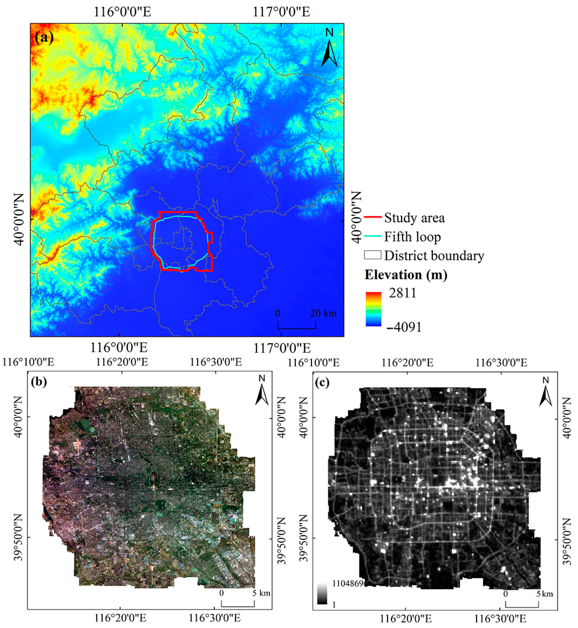
2.1. Study Area

Figure 1a presents a description of the research field in the central part of Beijing, China, within the 5th ring road area (116°10′–116°40′ E and 39°40′–40°10′ N), covering approximately 850 km². Beijing is recognized as the economic, political, and cultural center of China. Beijing’s urban area is encircled by ring roads that go around the forbidden city. The area’s western, northern, and northeastern sides encompass mountains, while the southeastern side slopes gently toward the Bohai Sea.

The LCZ classification system categorizes the study area with 2 primary categories and 17 sub-categories. While LCZs A to G are sparsely populated areas that are generally defined based on the type of ground cover, LCZs 1 to 10 are built-up areas that are mostly categorized based on their spatial morphological characteristics. The 17 LCZs meet the minimum categories for the global urban–rural study environment. It is possible to add or subtract from the LCZ classification when considering the local characteristics and to adjust the parameter ranges of some of these categories based on the local spatial morphology of the city. With regard to the urbanization process and characteristics of the study area, the 16 LCZ types employed in this investigation are listed in

Table 1. Table of LCZ classification systems.

LCZ Type	Schematic	LCZ Type	Schematic
LCZ-1 compact high-rise		LCZ-9 sparsely built
LCZ-2 compact mid-rise		LCZ-A dense trees
LCZ-3 compact low-rise		LCZ-B scattered trees
LCZ-4 open high-rise		LCZ-C bush or scrub
LCZ-5 open mid-rise		LCZ-D low plants
LCZ-6 open low-rise		LCZ-E bare rock or paved
LCZ-7 lightweight low-rise		LCZ-F bare soil or sand
LCZ-8 large low-rise		LCZ-G water

below [9].

2.2. Datasets

The Zhuhai-1 and Luojia-1 satellites collected, respectively, the day hyperspectral and night light pictures used in this investigation.

Table 2. Zhuhai-1 and Luojia-1 satellite parameters.

	Zhuhai-1	ALOS	Luojia-1
Spatial resolution (m)	10	12.5	130
Orbital altitude (km)	500	691.65	634
Weight (kg)	67	4000	20
Imaging range (km2)	150 × 2500	35 × 35	260 × 260
Number of spectral bands	32	4	1
Spectral range (nm)	400–1000	520–770	480–800
Operational orbit (°)	98	98.16	/

displays the main parameters of the Zhuhai-1 image and the Luojia-1 image.

The Zhuhai-1 image has 32 bands with coverage from 400 to 1000 nm and a resolution of 10 m. They provide rich spectral information for LCZ classification and help to distinguish ground features better. The cloud-free Zhuhai-1 images were acquired on 9 September and 1 November 2020, as shown in Figure 1b.

The DEM data source was made using a resampled 12.5 m resolution DEM that was formed based on ALOS satellite data.

The Luojia-1 satellite carries a high-sensitivity nighttime light camera with a 130 m ground resolution accuracy and a 260 km wide light imaging capability for the precise identification of roads and neighborhoods [29]. The Luojia-1 imagery used was collected in 2018, as shown in Figure 1c.

The road network was acquired in 2021 from the Open Street Map (OSM). We represented block boundaries using the network, with blocks considered the basic unit of the LCZ mapping [30,31]. As LCZs in parcels directly delineated by the OSM can be heterogeneous and mixed, we further divided the mixed zones into purer sub-blocks in order to label the attributes of the blocks. Finally, 7070 sub-districts were generated based on the road network. In order to manually interpret the ground reference of the LCZs based on the field survey, open-source geographic data sources such as sites of interest and street view pictures were used [32].

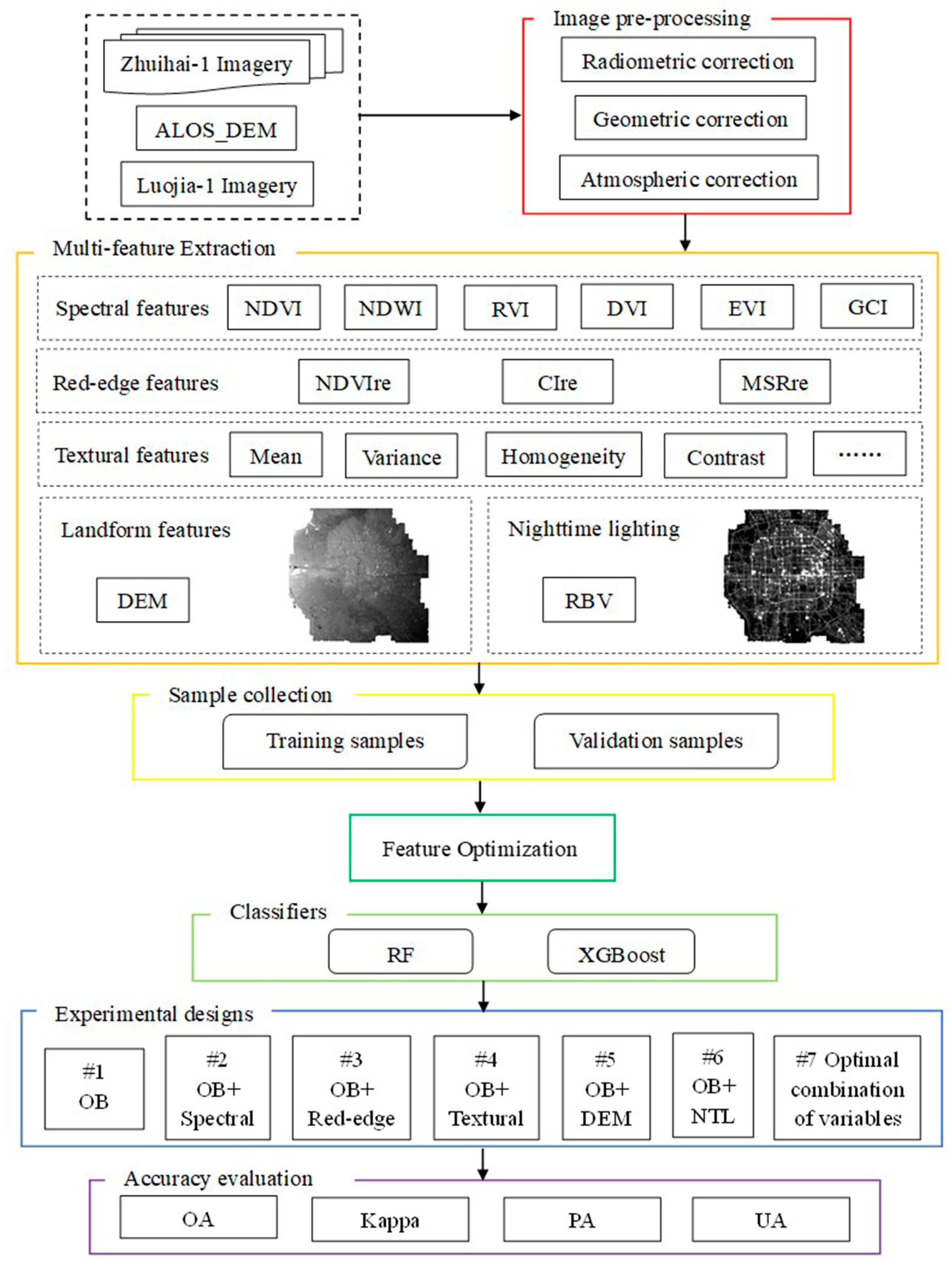
3. Methodology

Figure 2 depicts the six essential processes that make up the research workflow. (1) multi-feature extraction, including spectral, red-edge, textural, and landform features and nighttime lighting; (2) sample selection, categorized as training and validation datasets; (3) feature optimization, the optimal combination of variables for LCZ classification was selected using an average impurity reduction approach; (4) classifier use, in which the best combination of variables for LCZ classification was selected from two machine learning methods, namely random forest (RF) and XGBoost algorithms, in order to select the best classifier for LCZ classification; (5) experimental design, in which seven scenarios using different input features were designed; and (6) accuracy evaluation and the results of the analysis.

3.1. Multi-Feature Extraction

Feature extraction enables the full use of the Zhuhai-1 images’ rich spectral and spatial information.

Table 3. Detailed characterization of the indicators for this study.

Category	Feature	Input Band	Output Number of Features	Reference
Original band	Spectral information	B1, B2……B32	32	[23]
Spectral features	Normalized Difference Vegetation Index (NDVI)	NIR: B23-B29 R: B11-B14	28	[35]
	Normalized Difference Water Index (NDWI)	NIR: B23-B29 G: B3-B7	35	[36]
	Ratio Vegetation Index (RVI)	NIR: B23-B29 R: B11-B14	28	[37]
	Difference Vegetation Index (DVI)	NIR: B23-B29 R: B11-B14	28	[38]
	Enhanced Vegetation Index (EVI)	NIR: B23-B29 R: B11-B14 B: B1, B2	56	[39]
	Green Chlorophyll Vegetation Index (GCI)	NIR: B23-B29 G: B3-B7	35	[40]
Red-edge features	Red-edge Normalized Difference Vegetation Index (NDVIre)	NIR: B23-B29 RE: B15-B20	42	[41]
	Red-edge Chlorophyll Index (CIre)	NIR: B23-B29 RE: B15-B20	42
	Modified Red-edge Simple Ratio Index (MSRre)	NIR: B23-B29 RE: B15-B20	42
Textural features	Gray-level Co-occurrence Matrix (GLCM)	The first principal component of the Zhuhai-1 images	8	[23]
Landform features	Digital Elevation Model (DEM)	ALOS data resampling	1	/
Nighttime lighting	Radiation Brightness Value (RBV)	Luojia-1 Image	1	[32]

lists the features employed in this investigation, including spectral, red-edge, textural, and landform features and nighttime lighting, for the subsequent LCZ classification. As shown in the table, the original bands were the Zhuhai-1 data original bands (OBs) 1–32; the spectral features included NDVI, NDWI, RVI, DVI, EVI, and GCI. The red-edge features included NDVIre, CIre, and MSRre. The health of the plants is frequently evaluated using NDVIre, while the amount of chlorophyll in the canopy is determined using CIre. The distinct indicators of the gray-level co-occurrence matrix (GLCM) reflect distinct textural properties. On the Zhuhai-1 images, we ran a principal component analysis. To obtain the eigenvalues of the 32 principal components, we next used the covariance matrix approach. The first principal component was selected to calculate the GLCM, namely the mean, variance, homogeneity, contrast, dissimilarity, entropy, angular second moment, and correlation [23,33]. In particular, the landform feature DEM data source was made using a resampled 12.5m resolution DEM, formed based on ALOS satellite data. Finally, we extracted the nighttime lighting features, i.e., the radiometric brightness values (RBV) of Luojia-1 [34].

3.2. Sample Collection

We identified sixteen LCZ categories based on the spectral data from the Zhuhai-1 images and the field assessment of the research area. By using the high-resolution Zhuhai-1 images and Google Earth images with comparable imaging times, we classified the sample classes. The eigenvalues were obtained according to their properties from the respective sample blocks. Finally, the samples were split into 80% training and 20% validation using random sampling.

Table 4. Number of samples selected from the 16 local climate zones.

Type	Number of Training Samples	Number of Validation Samples
LCZ-1 compact high-rise	104	22
LCZ-2 compact mid-rise	172	44
LCZ-3 compact low-rise	229	63
LCZ-4 open high-rise	760	196
LCZ-5 open mid-rise	806	196
LCZ-6 open low-rise	474	106
LCZ-7 lightweight low-rise	35	19
LCZ-8 large low-rise	301	63
LCZ-9 sparsely built	370	76
LCZ-A dense trees	242	58
LCZ-B scattered trees	55	11
LCZ-C bush or scrub	48	12
LCZ-D low plants	394	108
LCZ-E bare rock or paved	852	230
LCZ-F bare soil or sand	599	159
LCZ-G water	215	51

shows the number of samples selected for the sixteen LCZ types.

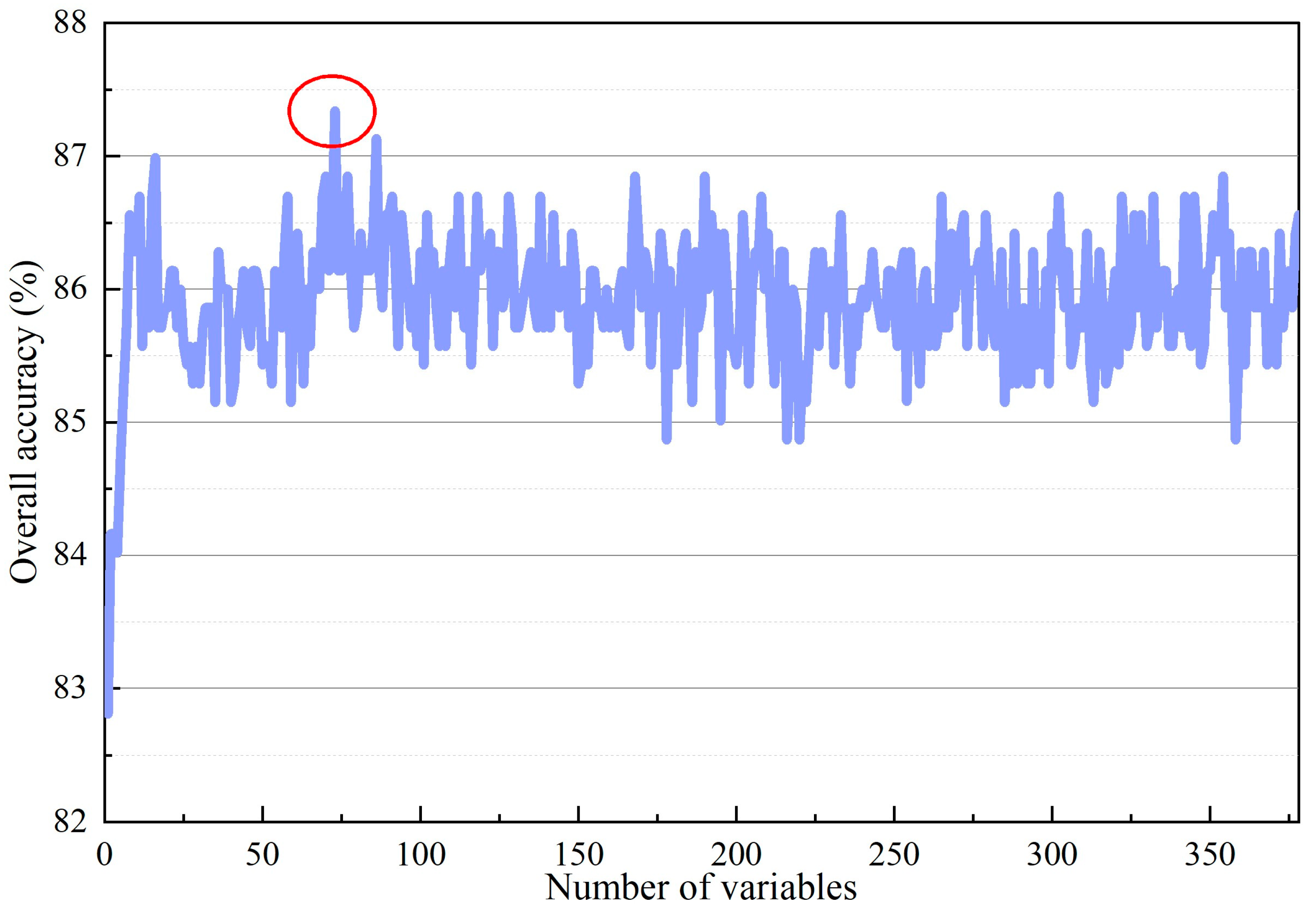
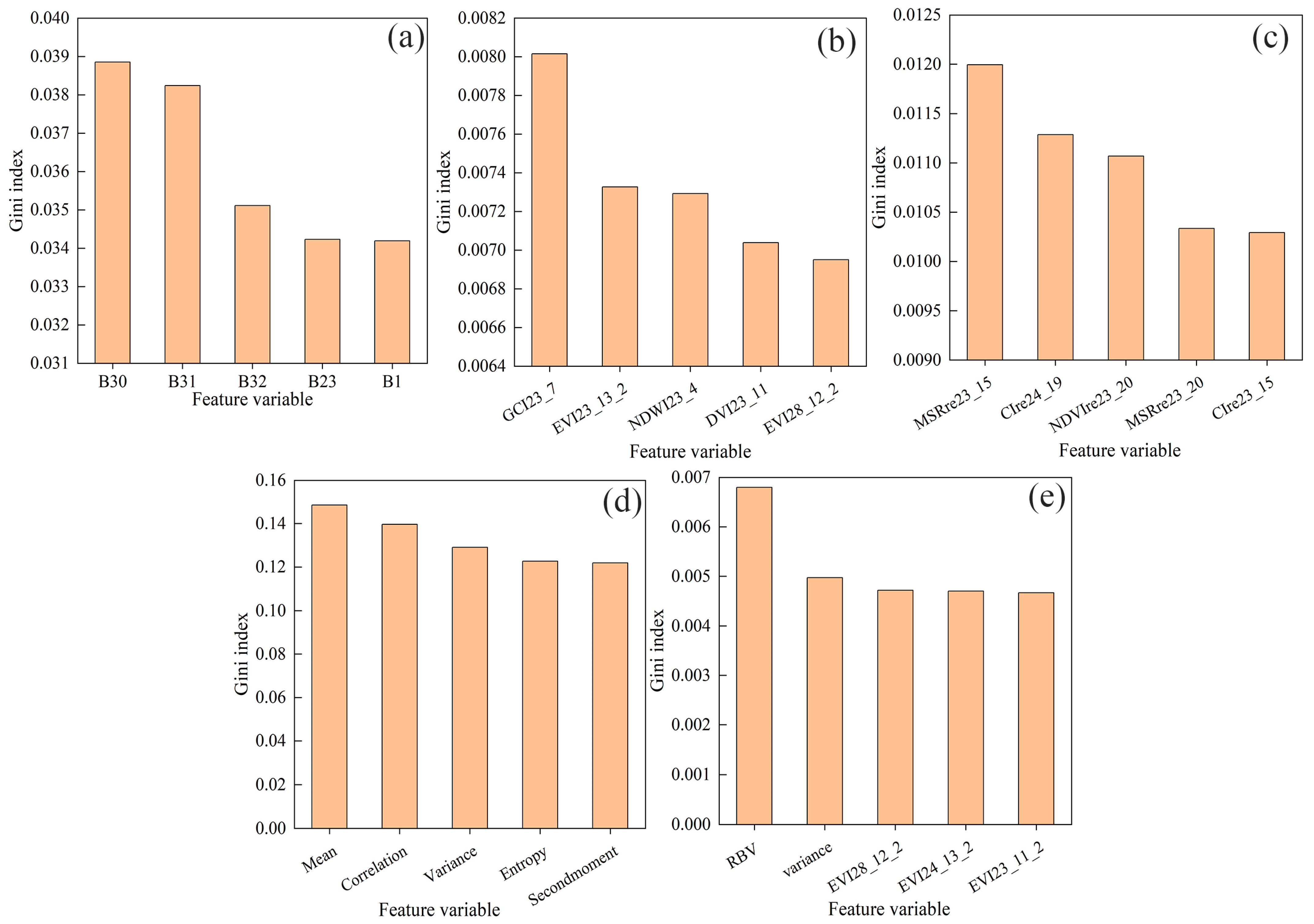
3.3. Feature Optimization

Feature optimization makes it possible to better comprehend the significance of the features and is essential to the avoidance of computational inefficiencies and to the improvement of the classification accuracy of high-dimensional data. We use the Gini index (GI) (i.e., the average reduction in impurities) to evaluate each variable’s significance [42]. The average error reduction for each feature is represented by the GI, which is calculated using the RF classifier’s structural data [43].

$$GI\left(P\right)={\sum }_{k=1}^K{P}_k\left(1-P_k\right)=1-{\sum }_{k=1}^K{P}_k^2$$

(1)

where P_k is the likelihood that the sample belongs to class k, k stands for the kth class, and GI(P) represents the GI value. Generally, a higher GI value denotes that the relevant variable has a significant influence on the classification. All the sample variable values were first extracted via the feature optimization stages. Secondly, the RF classifier was trained using the samples. Thirdly, the variable with the least importance was determined by ranking all the variables according to their GI values. Fourthly, the variables with the least importance were eliminated from the input parameters. The feature values of the newly combined variables for the sample were then retrieved and re-input into the RF classifier for training. The procedure was repeated until there were no more input variables. The variable terms and classification accuracies for each RF training were recorded during the iterative process. Finally, all the recorded accuracies were ranked to discover the optimal classification results and their corresponding variable terms, and the optimal variable combinations were output.

3.4. Classifiers

Two classifiers label LCZs, including Random Forest [44] and XGBoost [45].

(1)

Random forests have been extensively employed for categorization [46,47,48] and regression [49,50,51] in remote sensing. The recursive bifurcation method is used by the RF algorithm, which is based on categorical regression trees, to reach the tree structure’s final node [44]. Different decision trees can be used to train samples and forecast results in the RF classifier, which comprises many decision trees. Every tree generates its own prediction. The RF then integrates its votes to anticipate the result by computing the votes in each decision tree [52]. As a result, as compared to individual decision trees, the RF model can greatly enhance the classification results. Furthermore, the RF does well with outliers and noise, successfully avoiding overfitting [12]. Numerous fields have successfully used this technique with positive outcomes. The RF method is superior to many other methods in that it records full data with high accuracy, minimal grading, and no parameters [53].

(2)

The XGBoost (extreme gradient boosting) classifier is a tree-integration-based machine learning algorithm for binary or multiclassification problems. It is a gradient boosting framework that trains multiple weak classifiers and combines them into a single strong classifier to improve prediction accuracy. XGBoost uses an optimization algorithm that continuously adds new weak classifiers during training and optimizes the predictive power of each weak classifier using gradient boosting methods to minimize the loss function [45]. It can carry out multiple weak assessments of data collecting by condensing the modeling outcomes of the weak assessments. In addition, the XGBoost approach effectively handles classification and regression issues to produce more data than individual methods [54,55]. XGBoost also has an adaptive regularization capability to prevent overfitting and improve generalization ability [56]. Due to its efficiency and accuracy, one of the most widely used machine learning algorithms is XGBoost.

3.5. Experimental Design

We used the GI approach to optimize the features and then chose the top features for LCZ mapping. To further investigate how certain features affect LCZ classification, based on the outcomes of the feature optimization, we created seven alternative variable combination tests. The seven feature combination schemes were created to examine how different input feature variables performed in LCZ mapping. The feature combination schemes are detailed in

Table 5. Seven feature combination schemes for LCZ classification.

Experiment	Original Band	Spectral Features	Red-Edge Features	Textural Features	Landform Features	Nighttime Lighting
1	√
2	√	√
3	√		√
4	√			√
5	√				√
6	√					√
7	Optimal variables combination

. As shown in Table 5, Experiment 1 only used the original band as an input feature to assess how it affected LCZ mapping. Experiments 2 to 6 combined spectral, red-edge, textural, and landform features and nighttime lighting with the original bands to analyze and compare the roles of the added features in improving LCZ mapping accuracy. Exp. 7 included optimal variables for all feature classes, i.e., the original bands, spectral, red-edge, textural, and landform features and nighttime lighting, to explore the impact of multi-feature combinations on LCZ mapping.

3.6. Accuracy Evaluation

In order to properly analyze remote sensing image classification, accuracy evaluation is a crucial step which provides an important basis for analyzing the classification results [57]. To assess the precision of the LCZ classification, we used the confusion matrix [58]. A common method for evaluating accuracy, the confusion matrix primarily compares the level of misunderstanding between categorization results and actual measurements [59]. It has been widely used in studies on the classification of remote sensing images [60,61]. The confusion matrix displays the overall sample count for each category as well as the number of ordered and unreturned samples. The producer accuracy (PA), user accuracy (UA), overall accuracy (OA), and kappa coefficient, which show categorization accuracy from various perspectives, are the evaluation metrics of the confusion matrix. The overall classification accuracy is represented by the OA and kappa. The OA measures how many samples have been correctly identified out of all the samples. The kappa coefficient considers every component of the confusion matrix. With the UA commission error assessment and the PA omission error measurement, higher UA and PA indicate the categorization accuracy of specific categories [62].

4. Results

4.1. Results of Feature Optimization

We tested the varied OA values linked to various input variables, and Figure 3 shows the trend of OA with the input variables. The highest classification accuracy (OA = 87.34%) was achieved when the number of input variables was 73. OA increased rapidly as the input variables increased from 0 to 16. This indicates that with fewer input variables, the correlation between variables was negligible and that there was less redundancy when the classifier had higher classification efficiency and accuracy. As the number of input variables increased from 17 to 73, a slowly growing trend of OA was observed. The increase in the number of input variables from 74 to 378 caused the OA to stabilize. Due to increased data redundancy and correlation between factors, the performance of the classifier declined with an increase in the quantity of input variables. The efficiency and accuracy of classification also declined.

Table 6. Distribution of 73 optimal variables.

Feature	Optimal Variable Selection	Number
Original band	B2, B16, B30, B31	4
Spectral features	NDWI23_5, DVI23_13, EVI23_11_1, EVI23_11_2, EVI23_12_1, EVI23_12_2, EVI23_13_1, EVI23_13_2, EVI23_14_2, EVI24_11_1, EVI24_11_2, EVI24_12_1, EVI24_12_2, EVI24_13_1, EVI24_13_2, EVI24_14_1, EVI24_14_2, EVI25_11_1, EVI25_11_2, EVI25_12_1, EVI25_12_2, EVI25_13_1, EVI25_13_2, EVI25_14_1, EVI25_14_2, EVI26_11_1, EVI26_11_2, EVI26_12_2, EVI26_13_1, EVI26_13_2, EVI26_14_1, EVI26_14_2, EVI27_11_1, EVI27_11_2, EVI27_12_1, EVI27_12_2, EVI27_13_1, EVI27_13_2, EVI27_14_1, EVI27_14_2, EVI28_11_1, EVI28_11_2, EVI28_12_1, EVI28_12_2, EVI28_13_1, EVI28_13_2, EVI28_14_2, EVI29_11_2, EVI29_12_2, EVI29_13_1, EVI29_13_2, EVI29_14_1, EVI29_14_2, GCI23_5, GCI23_7, GCI28_4	56
Red-edge features	NDVIre24_19, CIre24_20, MSRre24_19	3
Textural features	Mean, Variance, Homogeneity, Contrast, Dissimilarity, Entropy, Second moment, Correlation	8
Landform features	DEM	1
Nighttime light	RBV	1

reveals the distribution of the 73 ideal variables, which included 4 original bands, 56 spectral features, 3 red-edge features, 8 texture features, 1 landform feature, and 1 nighttime light. Therefore, 73 variables were selected for the subsequent LCZ mapping.

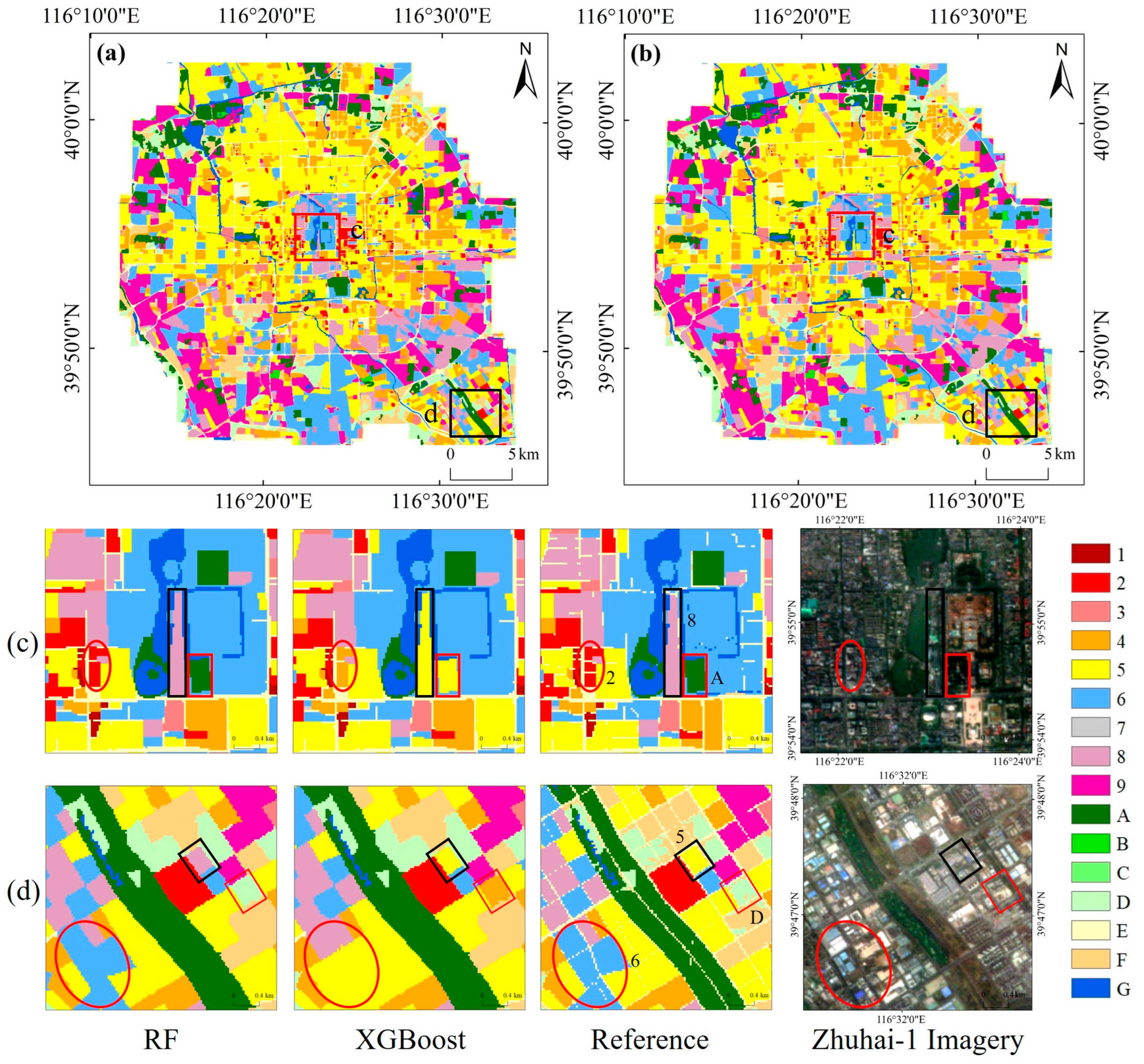
4.2. Results of LCZ Classification

Table 7. Results of LCZ classification accuracy of RF and XGBoost algorithm.

Type	RF		XGBoost
	PA (%)	UA (%)	PA (%)	UA (%)
1	72.73	100.00	84.21	88.89
2	81.82	100.00	74.47	100.00
3	77.78	100.00	78.46	100.00
4	89.29	81.02	87.98	80.90
5	83.67	83.67	89.83	85.95
6	84.91	90.91	81.82	86.09
7	100.00	100.00	100.00	100.00
8	88.89	93.33	83.33	87.30
9	89.47	85.00	89.80	84.62
A	89.66	89.66	76.79	82.69
B	100.00	100.00	100.00	100.00
C	100.00	100.00	100.00	100.00
D	87.96	95.96	82.80	82.80
E	92.17	84.13	88.99	82.55
F	83.65	81.10	86.67	89.14
G	92.16	100.00	84.31	87.76
OA (%)	87.34		86.07
Kappa	0.86		0.85

displays the LCZ classification accuracy using the RF and XGBoost classifiers. The table shows that with an OA value of 87.34% and a kappa coefficient of 0.86 the RF classifier produced the highest level of accuracy. The XGBoost classifier had slightly lower classification accuracy (OA value of 86.07% and a kappa coefficient of 0.85). In conclusion, the RF classifier outperformed the XGBoost classifier in terms of accuracy and had a clear advantage in recognizing LCZs.

Figure 4a,b display the results of the LCZ categorization utilizing the ideal combination of the RF and XGBoost classifier variables. Two sub-regions were chosen in order to show their differences in spatial classification detail (Figure 4c,d). The red rectangle shown in Figure 4c is LCZ-A (dense trees), and the black rectangle gives an example of LCZ-8 (large low-rise). We found that the two blocks were well identified using the RF classifier; however, the XGBoost classifier misclassified them as LCZ-5 (open mid-rise). Similarly, the red circle in Figure 4c gives an example of LCZ-2 (compact mid-rise) and shows that the RF classifier could accurately classify that location; however, the XGBoost classifier incorrectly classified it as LCZ-4 (open high-rise). In addition, the red rectangle in Figure 4d shows LCZ-D (low plants). The RF classifier identified the block well but used the XGBoost classifier to incorrectly classify it as LCZ-4. In Figure 4d, the red circle shows LCZ-6 (open low-rise), which the RF classifier identified correctly. Still, the XGBoost classification incorrectly identified the block as LCZ-5 and LCZ-8. An example of an LCZ-5 is given in the black rectangle in Figure 4d, showing that the XGBoost classifier could identify the block well. Still, the RF classification incorrectly misclassified it as LCZ-8. Therefore, based on the above analysis, the RF classifier is better suited to LCZ classification.

4.3. Classification Results for Multi-Feature Combinations

In this study, Zhuhai-1 images, a fresh supply of high spectral resolution data, and the feature indices that were produced from them, i.e., spectral features, red-edge features, and textural features, fused with ALOS_DEM images and Luojia-1 nighttime light data, were used for the LCZ classification study. To examine the impact of various the feature indices on the precision of the LCZ classification, six unoptimized schemes were developed (Table 6). Figure 5 shows the OA of seven feature combinations using both RF and XGBoost classifiers. Exp1 used only the original bands as input features, and the RF and XGBoost algorithms achieved OAs of 82.96% and 80.83%, respectively. Exps 2 to 6 combined spectral, red-edge, textural, and landform features and nighttime lights with the original bands, respectively. The OA improved for both classifiers when the original bands were combined with the additional features. Compared to the original bands alone, the OAs of the RF algorithm increased by 2.33%, 1.34%, 2.19%, 1.91%, and 1.91%, respectively, and the OAs of XGBoost increased by 4.60%, 4.17%, 4.38%, 1.98%, and 2.26%, accordingly. These findings demonstrate how the accuracy of LCZ classification was considerably increased by the spectral and textural data. Landform features and nighttime lighting were effective in enhancing the LCZ classification accuracy. These results are consistent with those of earlier research [27,32,63]. Exp7 included optimal variables for all feature classes, i.e., original band; spectral, red-edge, textural, and landform feature DEM; and NTL. Both classifiers achieved the highest accuracies of 87.34% and 86.07%, respectively. It can be concluded that multi-feature fusion improves LCZ mapping accuracy.

Combining OBs and spectral features produced the most accurate results out of the six unoptimized techniques (Figure 5). Spectral features are an important indicator for vegetation monitoring as they identify vegetation and non-vegetation and capture different vegetation types. Furthermore, combining optimized variables solved the data redundancy problem and significantly improved the classification accuracy of the LCZ (Figure 5). The classification accuracy was highest with a kappa coefficient of 0.86 and an OA of 87.34%. Figure 6 shows a zoomed-in view of the LCZ results for the seven scenarios using RF classifiers. Among the six unoptimized schemes, the LCZ mapping of Exp2 performed well (Figure 6b), while Exp7 outperformed the others (Figure 6g).

The classification outcomes for the six studies utilizing the RF classifier are displayed in Figure 7. The classification accuracy results for the six systems are illustrated in detail in Figure 8. Figure 5 shows the extent of the OA from 82.96% to 85.29%, indicating that the input features influence the accuracy of LCZ classification.

(1)

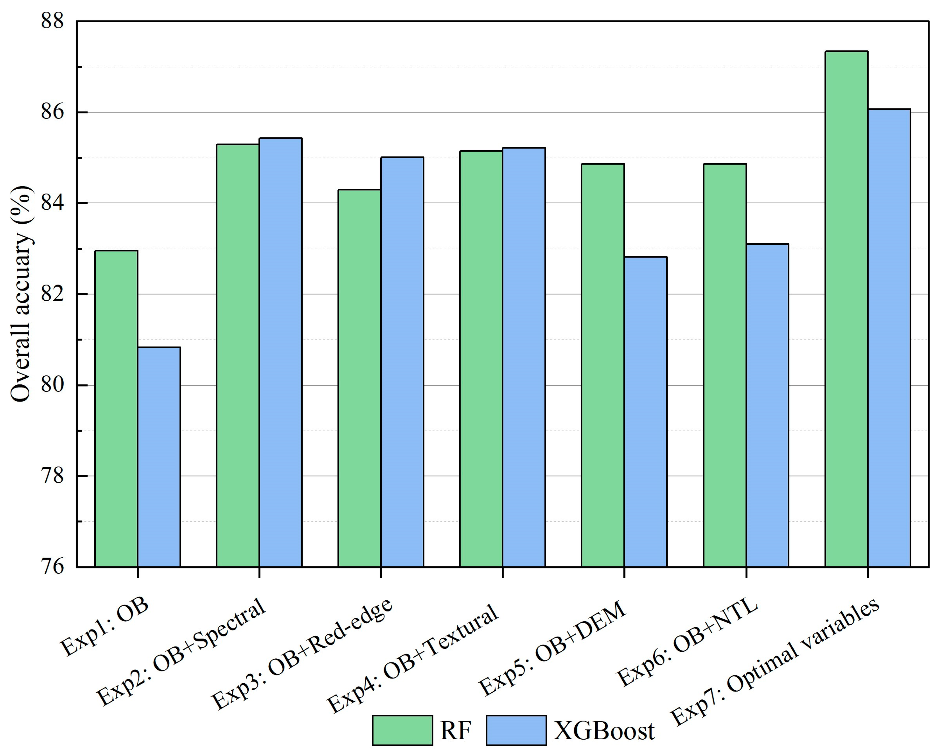
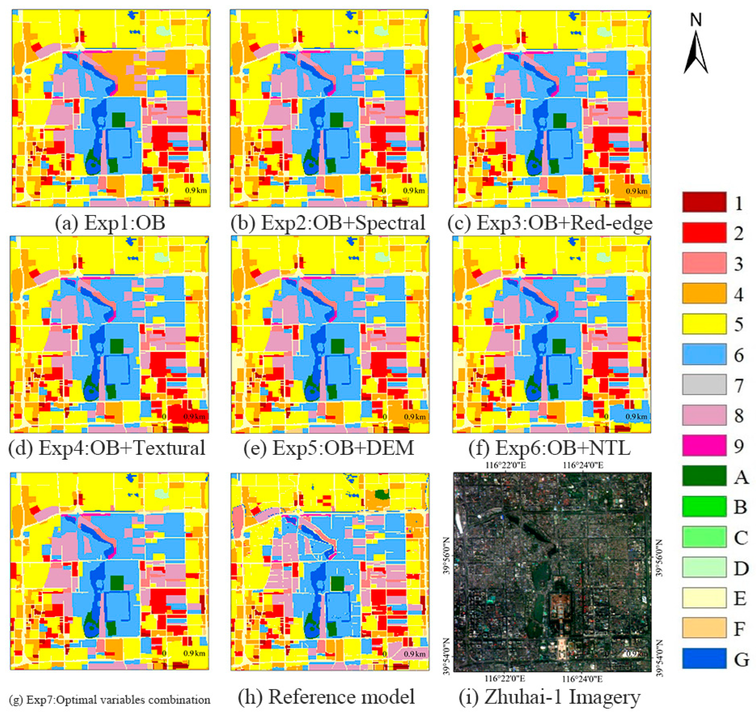
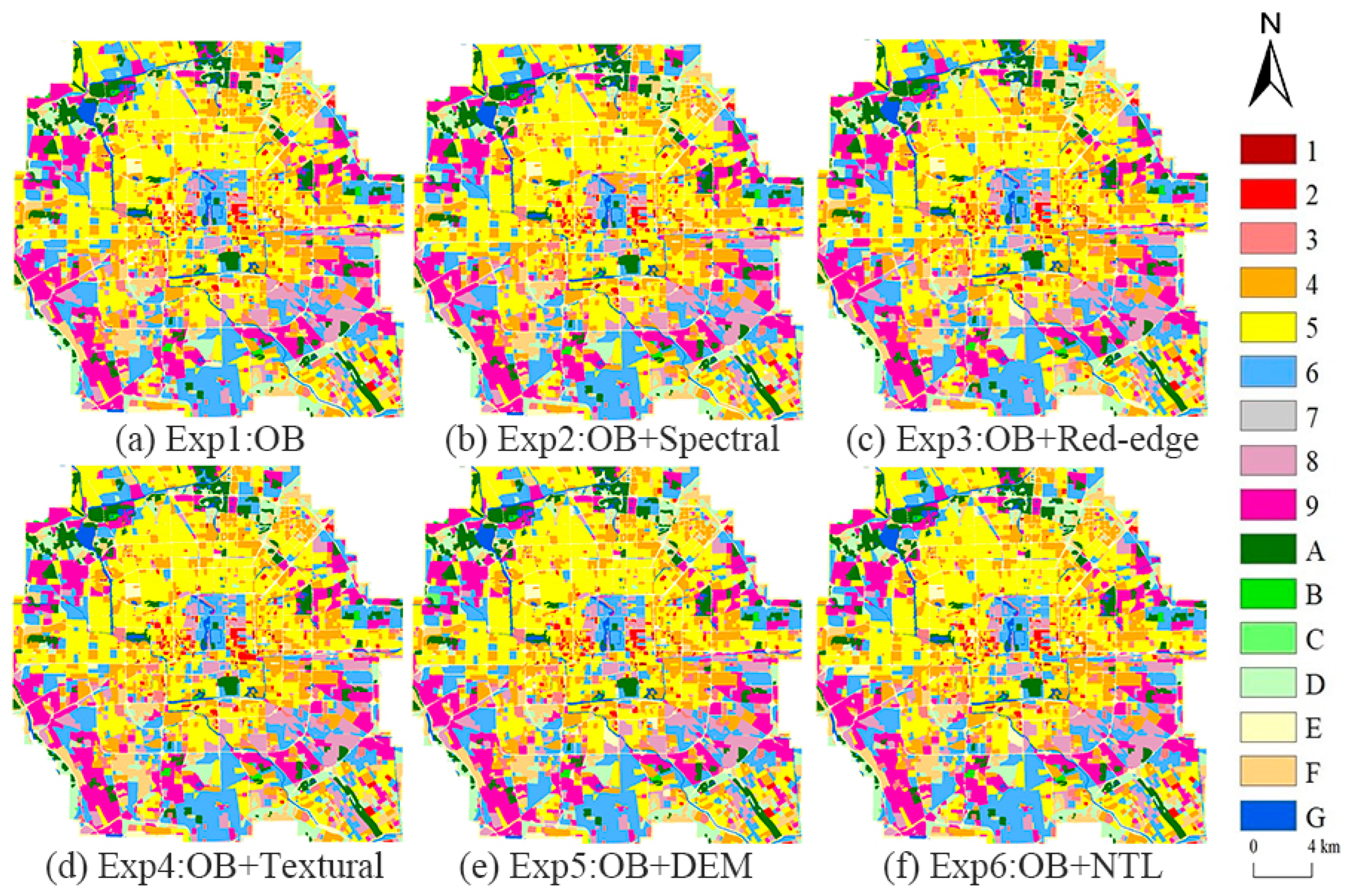
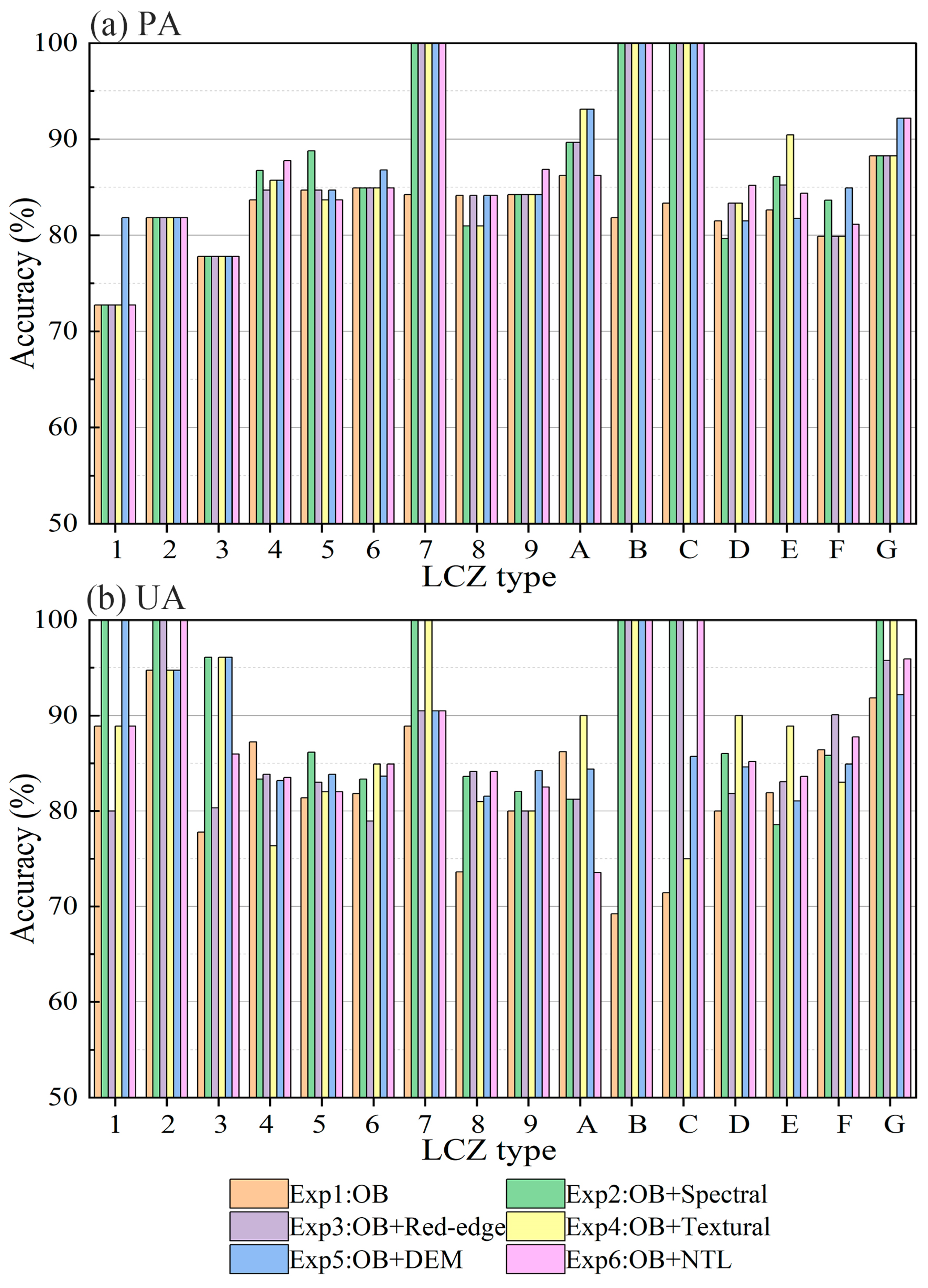
Exp1, which used only the original bands as an input feature, showed the lowest classification accuracy (Exp1: OA = 82.96%, kappa coefficient = 0.81). Most LCZs had PA values above 80%, except for LCZ-1 (compact high-rise), LCZ-3 (compact low-rise), and LCZ-F (bare soil and sand). The UA of LCZ-2 (compact mid-rise) and LCZ-G (water) exceeded 90%.

(2)

With regard to the six scenarios, Exp2’s original bands and spectral properties had the best classification accuracy (Exp2: OA = 85.29%, kappa coefficient = 0.84). Aside from that, LCZ-5 (open mid-rise) had the highest PA compared to the other experiments. The UA of Exp2 reached 100% in LCZ-1, LCZ-2, LCZ-7 (lightweight low-rise), LCZ-B (scattered trees), LCZ-C (bush or scrub), and LCZ-G. Similarly, the accuracy of the original bands combined with the textural features as input features in Exp4 was second only to Exp2 (Exp4: OA = 85.15%, kappa coefficient = 0.83). The GLCM helped to improve the PA of LCZ-A (dense trees) and LCZ-E (bare rock or paved). The UA of Exp4 reached 100% in LCZ-7, LCZ-B, and LCZ-G. In conclusion, the accuracy of the LCZ classification was greatly increased by spectral and textural features.

(3)

Exp5 used a combination of original bands and landform feature DEMs as input features for classification (Exp5: OA = 84.87%, kappa coefficient = 0.83). The DEM in Exp5 helped to improve the PA of LCZ-1, LCZ-6 (open low-rise), LCZ-A, LCZ-F, and LCZ-G. The UA of Exp5 reached 100% in LCZ-1 and LCZ-B. Similarly, Exp6 used original bands combined with nighttime lights as input features; only Exp5 had the same accuracy. However, the RBV in Exp6 helped to improve the PA of LCZ-4 (open high-rise), LCZ-9 (sparsely built), LCZ-D (low plants), and LCZ-G. The UA of Exp6 reached 100% in LCZ-2, LCZ-B, and LCZ-C.

(4)

Exp3 combined the original bands and red-edge features as input features with slightly lower classification accuracy (Exp5: OA = 84.30%, kappa coefficient = 0.83). The UA of Exp3 reached 100% for LCZ-2, LCZ-B, and LCZ-C.

5. Discussion

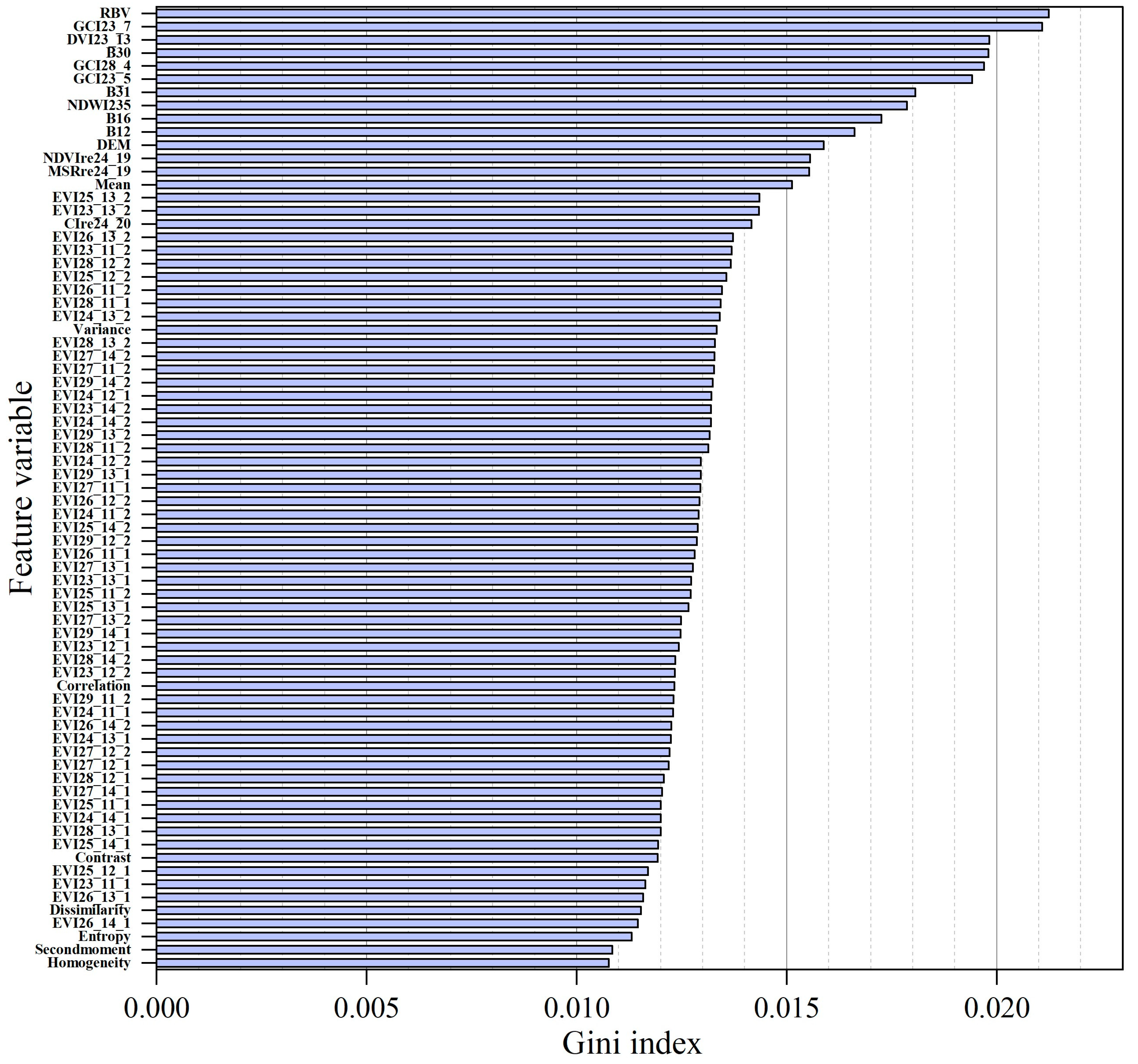
5.1. Variable Importance Analysis

It was necessary to investigate the significance of factors for the LCZ classification due to the high spectral resolution of the Zhuhai-1 images. In order to analyze the variable relevance of each feature class, we used the Gini index approach. Figure 9a–e illustrate the top five significant variables for the original bands, spectral features, red-edge features, textural features, and all input variables. Of the original bands, the NIR bands B30, B31, B32, and B23 and the blue band B1 were the most crucial factors in LCZ classification, indicating that the NIR bands played a crucial role in LCZ classification. GCI23_7, calculated from the green band B7 and the NIR band B23, was the key factor affecting the spectral characteristics. The key variables in the red-edge features were MSRre23_15, CIre24_19, and NDVIre23_20. In addition, the GLCM was ranked in order of importance as mean > correlation > variance > entropy > second moments. The first five input variables are shown in Figure 9e. The variation in textural features, the three EVIs, and RBV were the three most crucial variables. Each classification scheme had a different set of correlations between its variables since two or more feature variables made up the input variables. The relative importance of the variables was ranked in this manner in this study. The mean, for instance, is the most crucial variable in Figure 9d’s texture feature, whereas Figure 9f’s variance is the variable that performs the best overall.

Figure 10 shows the importance ranking of the 73 optimal variables in the LCZ classification. First, RBV (GI value = 0.0212) attained the classification’s highest variable importance value, indicating that night lighting strongly influences LCZ classification. GCI23_7 had a GI value of 0.0211, and DVI23_13 also produced a high GI value (0.0198), demonstrating the importance of vegetation indices for LCZ mapping. The DEM also produced a high GI value (0.0159), indicating that landform features strongly influence LCZ classification. The original bands had better classification performance (they all had GI values above 0.016); the textural features had relatively low GI values (most of them had GI values below 0.015). In summary, the variables in descending order of importance are nighttime lighting > original bands > landform feature > red-edge features > spectral features > textural features.

5.2. Comparison with Existing Methods

LCZ classification using remotely sensed data has been the subject of numerous prior studies, and many researchers have concentrated on introducing new data sources or classification techniques [23,24,26,64,65,66]. Furthermore, the accuracy of LCZ classification can be greatly improved by using the specific measurements that the derived features offer to identify features. Because of this, it is essential to investigate the potential and worth of novel remote sensing data sources and their derivation features in LCZ classification applications. This study combined a new multi-source remote sensing data combination approach; Zhuhai-1 images, ALOS_DEM data, and Luojia-1 images with their derived feature indices, i.e., spectral features, red-edge features, textural features, landform features, and nighttime lights, were used in the LCZ classification studies. While previous studies have only enabled features such as spectral and textural features for LCZ classification, our approach considered the potential of red-edge features, landform features, and nighttime lights, i.e., NDVIre, CIre, MSRre, DEM, and RBV for LCZ classification, as different LCZs essentially produce heterogeneity. Our results confirm that adding new features can significantly improve the OA value of the LCZ.

We compared the proposed strategy with the data sources and evaluation results (i.e., OA values), using current state-of-the art models to demonstrate the benefits of our approach more clearly (

Table 8. Comparison of existing LCZ classification methods.

Methodology	Data Source	Study Area	Overall Accuracy	References
Machine learning random forest algorithm	Landsat and ASTER data and their GLCM	Guangzhou and Wuhan, China	66%, 84%	[23]
An ensemble classifier	Data products for Sentinel-1 Level-1 Dual-Pol	Global scale, 29 cities	61.8%	[24]
Residual convolutional neural network (ResNet)	Sentinel-2 and Landsat-8 images and the VIIRS-based NTL data	Nine cities in Europe	78%	[26]
The semi-automatic algorithm	Building information, land use data, and remote sensing images from Landsat 8	Chenzhou, China	69.54%	[64]
Supervised convolutional neural networks (CNNs)	Multi-temporal Sentinel-2 composites	Eight German cities	86.5%	[65]
WUDAPT (level 0) method	Landsat 5 satellite images	Hong Kong, China	58%	[66]
Our method	Zhuhai-1 images, ALOS_DEM data, Luojia-1 nighttime lighting data	Beijing, China	87.34%	/

). Our approach produced more respectable evaluation results (OA value = 87.34%) compared to those of most strategies. Second, the major goal of LCZ categorization is to make the most of the variations in spectral properties, spatial patterns of objects, and textural features among the different LCZs, bearing in mind that other tactics and metrics could cost more. Our method requires Zhuhai-1 images, ALOS-DEM images, and Luojia-1 images to be freely available. Based on the foregoing description, our method, with its higher accuracy and cheaper cost, is ideal for accurate LCZ classification.

As previously stated, by considering different feature combinations, this study used an accurate technique for LCZ classification. There are, however, several drawbacks to be aware of. The importance of additional features in LCZ mapping is first highlighted in this study. However, more variables are needed to obtain good LCZ classification findings in cities with complex and varied environments. Second, different activities are often carried out in diverse LCZs and are connected to socio-economic events. For LCZ mapping, open social data about human activities are useful. To enable more precise LCZ mapping, future research must investigate other features that are already available and that include open social data.

Although spectral, red-edge, and texture features from Zhuhai-1 imagery, ALOS_DEM data, and nighttime light data from Luojia-1 were incorporated in this study, other relevant variables may improve the model’s performance. Exploring the inclusion of additional variables, such as meteorological data, topographic features, or surface temperature, could provide valuable information to capture local climate features better and improve LCZ mapping accuracy. The success of the method relies on the availability and quality of the input data. In some regions or countries, obtaining high-resolution hyperspectral imagery, accurate DEMs, and reliable nighttime light data may pose challenges. Future work could focus on addressing data limitations by exploring alternative data sources, such as open satellite imagery or aerial surveys, and improving data quality through pre-processing techniques and data fusion methods. Although the method has shown good accuracy in the central Beijing area, its generalizability to other regions, especially those with unique climatic and environmental conditions, needs further investigation. Future studies should aim to assess the performance of the method in different urban contexts, considering variations in land cover types, urban forms, and climate patterns. This may involve conducting case studies in different regions and assessing the transferability of the method to ensure its broader applicability.

6. Conclusions

In this research, we suggested a brand-new LCZ mapping technique for merging diurnal data from many remote sensing sources, i.e., fusing daytime Zhuhai-1 hyperspectral images and their derived feature indices, ALOS_DEM data, and Luojia-1 nighttime lighting data; we validated the method in Beijing, China and explored the potential of each feature in LCZ mapping. We considered all possible combinations of bands to obtain features and enhance LCZ classification to evaluate the full range of useful information from the Zhuhai-1 images. We devised feature optimization methods to reduce redundancy and improve LCZ classification accuracy. In addition, to examine and contrast the impacts of various input features on the LCZ classification accuracy, we created six classification schemes and used RF and XGBoost classifiers. The following are the study’s principal conclusions.

(1)

Our findings demonstrate the method’s superb LCZ mapping accuracy. The RF classifier had a kappa coefficient of 0.86 and the greatest OA (87.34%). The classification accuracy of the XGBoost classifier was marginally lower (OA value of 86.07% and kappa coefficient of 0.85). In a word, the RF classifier outperformed the XGBoost classifier in terms of accuracy and had a clear advantage in recognizing LCZs.

(2)

Using only the original bands as input features, the RF and XGBoost algorithms achieved OAs of 82.96% and 80.83%, respectively. The results of the study showed that the accuracies of LCZ classification in terms of spectral and textural features were improved by 2.33% and 2.19% using the RF classifier, respectively.

(3)

With a GI value of 0.0212, the variable importance analysis revealed that RBV was the variable that had the greatest impact on LCZ classification. The DEM also yielded a high GI value (0.0159). The feature indices were ranked in order of importance as nighttime lights > original bands > landform features > red-edge features > spectral features > textural features.

Our study offers a fresh viewpoint on LCZ mapping and emphasizes that NTL and landform feature DEMs should be considered in future LCZ mapping studies.

References

- Cao, S.; Cai, Y.; Du, M.; Weng, Q.; Lu, L. Seasonal and diurnal surface urban heat islands in China: An investigation of driving factors with three-dimensional urban morphological parameters. GIScience Remote Sens. 2022, 59, 1121–1142. [Google Scholar] [CrossRef]
- Kamali Maskooni, E.; Hashemi, H.; Berndtsson, R.; Daneshkar Arasteh, P.; Kazemi, M. Impact of spatiotemporal land-use and land-cover changes on surface urban heat islands in a semiarid region using Landsat data. Int. J. Digit. Earth 2021, 14, 250–270. [Google Scholar] [CrossRef]
- Lee, Y.Y.; Din, M.F.M.; Ponraj, M.; Noor, Z.Z.; Iwao, K.; Chelliapan, S. Overview of Urban Heat Island (UHI) phenomenon towards human thermal comfort. Environ. Eng. Manag. J. 2017, 16, 2097–2112. [Google Scholar] [CrossRef]
- Stewart, I.D. A systematic review and scientific critique of methodology in modern urban heat island literature. Int. J. Climatol. 2011, 31, 200–217. [Google Scholar] [CrossRef]
- Voogt, J.A.; Oke, T.R. Thermal remote sensing of urban climates. Remote Sens. Environ. 2003, 86, 370–384. [Google Scholar] [CrossRef]
- Li, G.; Zhang, J.; Cheng, H.; Zhao, L.; Tian, H. Urban Heat Island Effect against the Background of Global Warming and Urbanization. Prog. Meteorol. Sci. Technol. 2012, 6, 45–49. [Google Scholar]
- Manley, G. On the frequency of snowfall in metropolitan England. Q. J. R. Meteorolog. Soc. 1958, 84, 70–72. [Google Scholar] [CrossRef]
- Mills, G.; Bechtel, B.; Ching, J.; See, L.; Feddema, J.; Foley, M.; Alexander, P.; O’Connor, M. An Introduction to the WUDAPT project. In Proceedings of the 9th International Conference on Urban Climate (ICUC9), Toulouse, France, 20–24 July 2015; p. 6. [Google Scholar]
- Stewart, I.D.; Oke, T.R. Local climate zones for urban temperature studies. Bull. Am. Meteorol. Soc. 2012, 93, 1879–1900. [Google Scholar] [CrossRef]
- Alberti, M.; Weeks, R.; Coe, S. Urban land-cover change analysis in Central Puget Sound. Photogramm. Eng. Remote Sens. 2004, 70, 1043–1052. [Google Scholar] [CrossRef] [Green Version]
- Kane, K.; Tuccillo, J.; York, A.M.; Gentile, L.; Ouyang, Y. A spatio-temporal view of historical growth in Phoenix, Arizona, USA. Landsc. Urban Plann. 2014, 121, 70–80. [Google Scholar] [CrossRef]
- Yao, Y.; Li, X.; Liu, X.; Liu, P.; Liang, Z.; Zhang, J.; Mai, K. Sensing spatial distribution of urban land use by integrating points-of-interest and Google Word2Vec model. Int. J. Geog. Inf. Sci. 2017, 31, 825–848. [Google Scholar] [CrossRef]
- Johnston, R.B. Arsenic and the 2030 Agenda for sustainable development. In Arsenic Research and Global Sustainability—Proceedings of the 6th International Congress on Arsenic in the Environment, AS 2016, Stockholm, Sweden, 19–23 June 2016; CRC Press: Boca Raton, FL, USA, 2016; pp. 12–14. [Google Scholar] [CrossRef]
- Danylo, O.; See, L.; Gomez, A.; Schnabel, G.; Fritz, S. Using the LCZ framework for change detection and urban growth monitoring. EGU Gen. Assem. Conf. Abstr. 2017, 19, 18043. [Google Scholar]
- Bechtel, B.; Conrad, O.; Tamminga, M.; Verdonck, M.L.; Van Coillie, F.; Tuia, D.; Demuzere, M.; See, L.; Lopes, P.; Fonte, C.C.; et al. Beyond the urban mask: Local climate zones as a generic descriptor of urban areas—Potential and recent developments. In Proceedings of the 2017 Joint Urban Remote Sensing Event (JURSE), Dubai, United Arab Emirates, 6–8 March 2017; pp. 1–4. [Google Scholar]
- Ching, J.; Mills, G.; See, L.; Bechtel, B.; Feddema, J.; Stewart, I.; Wang, X.; Ng, E.; Ren, C.; Brousse, O.; et al. Wudapt (World Urban Database and Access Portal Tools): An International Collaborative Project for Climate Relevant Physical Geography Data for the World‘s Cities. In Proceedings of the 96th Amercian Meteorological Society Annual Meeting, New Orleans, LA, USA, 10–14 January 2016; pp. 1–7. [Google Scholar]
- Feddema, J.; Mills, G.; Ching, J. Demonstrating the Added Value of WUDAPT for Urban Climate Modelling. In Proceedings of the ICUC9, Toulouse, France, 20–24 July 2015; Volume 19, p. 15889. [Google Scholar]
- Bechtel, B.; Alexander, P.J.; Böhner, J.; Ching, J.; Conrad, O.; Feddema, J.; Mills, G.; See, L.; Stewart, I. Mapping local climate zones for a worldwide database of the form and function of cities. ISPRS Int. J. Geo-Inf. 2015, 4, 199–219. [Google Scholar] [CrossRef] [Green Version]
- Ren, C.; Cai, M.; Li, X.; Zhang, L.; Wang, R.; Xu, Y.; Ng, E. Assessment of Local Climate Zone Classification Maps of Cities in China and Feasible Refinements. Sci. Rep. 2019, 9, 18848. [Google Scholar] [CrossRef] [PubMed] [Green Version]
- Bechtel, B.; Daneke, C. Classification of local climate zones based on multiple earth observation data. IEEE J. Sel. Top. Appl. Earth Obs. Remote Sens. 2012, 5, 1191–1202. [Google Scholar] [CrossRef]
- Gál, T.; Bechtel, B.; Unger, J. Comparison of two different local climate zone mapping methods. In Proceedings of the ICUC9-9th International Conference on Urban Climates, Toulouse, France, 20–24 July 2015; pp. 1–6. [Google Scholar]
- Liu, S.; Shi, Q. Local climate zone mapping as remote sensing scene classification using deep learning: A case study of metropolitan China. ISPRS J. Photogramm. Remote Sens. 2020, 164, 229–242. [Google Scholar] [CrossRef]
- Xu, Y.; Ren, C.; Cai, M.; Edward, N.Y.Y.; Wu, T. Classification of Local Climate Zones Using ASTER and Landsat Data for High-Density Cities. IEEE J. Sel. Top. Appl. Earth Obs. Remote Sens. 2017, 10, 3397–3405. [Google Scholar] [CrossRef]
- Hu, J.; Ghamisi, P.; Zhu, X.X. Feature Extraction and Selection of Sentinel-1 Dual-Pol Data for Global-Scale Local Climate Zone Classification. ISPRS Int. J. Geo-Inf. 2018, 7, 379. [Google Scholar] [CrossRef] [Green Version]
- He, S.; Zhang, Y.; Gu, Z.; Su, J. Local climate zone classification with different source data in Xi’an, China. Indoor Built Environ. 2019, 28, 1190–1199. [Google Scholar] [CrossRef]
- Qiu, C.; Schmitt, M.; Mou, L.; Ghamisi, P.; Zhu, X.X. Feature importance analysis for local climate zone classification using a residual convolutional neural network with multi-source datasets. Remote Sens. 2018, 10, 1572. [Google Scholar] [CrossRef] [Green Version]
- Mo, Y.; Zhong, R.; Cao, S. Orbita hyperspectral satellite image for land cover classification using random forest classifier. J. Appl. Remote Sens. 2021, 15, 014519. [Google Scholar] [CrossRef]
- Chen, C.; Bagan, H.; Xie, X.; La, Y.; Yamagata, Y. Combination of sentinel-2 and palsar-2 for local climate zone classification: A case study of nanchang, China. Remote Sens. 2021, 13, 1902. [Google Scholar] [CrossRef]
- Ou, J.; Liu, X.; Liu, P.; Liu, X. Evaluation of Luojia 1-01 nighttime light imagery for impervious surface detection: A comparison with NPP-VIIRS nighttime light data. Int. J. Appl. Earth Obs. Geoinf. 2019, 81, 1–12. [Google Scholar] [CrossRef]
- Shin, H.B. Residential redevelopment and the entrepreneurial local state: The implications of Beijing’s shifting emphasis on urban redevelopment policies. Urban Stud. 2009, 46, 2815–2839. [Google Scholar] [CrossRef] [Green Version]
- Zhao, P.; Lü, B. Transportation implications of metropolitan spatial planning in mega-city Beijing. Int. Dev. Plan. Rev. 2009, 31, 235–261. [Google Scholar] [CrossRef]
- Huang, X.; Yang, J.; Li, J.; Wen, D. Urban functional zone mapping by integrating high spatial resolution nighttime light and daytime multi-view imagery. ISPRS J. Photogramm. Remote Sens. 2021, 175, 403–415. [Google Scholar] [CrossRef]
- Haralick, R.M.; Dinstein, I.H.; Shanmugam, K. Textural Features for Image Classification. IEEE Trans. Syst. Man Cybern. 1973, SMC-3, 610–621. [Google Scholar] [CrossRef] [Green Version]
- Zhang, R.; Huang, C.; Zhan, X.; Jin, H.; Song, X.P. Development of S-NPP VIIRS global surface type classification map using support vector machines. Int. J. Digit. Earth 2018, 11, 212–232. [Google Scholar] [CrossRef]
- Jiang, Z.; Huete, A.R.; Chen, J.; Chen, Y.; Li, J.; Yan, G.; Zhang, X. Analysis of NDVI and scaled difference vegetation index retrievals of vegetation fraction. Remote Sens. Environ. 2006, 101, 366–378. [Google Scholar] [CrossRef]
- McFeeters, S.K. The use of the Normalized Difference Water Index (NDWI) in the delineation of open water features. Int. J. Remote Sens. 1996, 17, 1425–1432. [Google Scholar] [CrossRef]
- Priebe, S.; Huxley, P.; Knight, S.; Summary, S.E. Application and Results of the Manchester Short Assessment of Quality of Life (Mansa). Int. J. Soc. Psychiatry 1999, 45, 7–12. [Google Scholar] [CrossRef] [PubMed] [Green Version]
- Tucker, C.J. Red and photographic infrared linear combinations for monitoring vegetation. Remote Sens. Environ. 1979, 8, 127–150. [Google Scholar] [CrossRef] [Green Version]
- Stewart, I.D.; Oke, T.R.; Bechtel, B.; Foley, M.M.; Mills, G.; Ching, J.; See, L.; Alexander, P.J.; O’Connor, M.; Albuquerque, T.; et al. Generating WUDAPT’s Specific Scale -dependent Urban Modeling and Activity Parameters: Collection of Level 1 and Level 2 Data. In Proceedings of the ICUC9, Toulouse, France, 20–24 July 2015; Volume 5, pp. 1–4. [Google Scholar]
- Gitelson, A.A.; Gritz, Y.; Merzlyak, M.N. Relationships between leaf chlorophyll content and spectral reflectance and algorithms for non-destructive chlorophyll assessment in higher plant leaves. J. Plant Physiol. 2003, 160, 271–282. [Google Scholar] [CrossRef] [PubMed]
- Thenkabail, P.S.; Smith, R.B.; De Pauw, E. Wiegand and Richardson, † International Center for Agricultural Research in the Dry Areas 1990), natural vegetation (Friedl et al., 1994), and in (ICARDA). Environ 1995, 71, 158–182. [Google Scholar]
- Strobl, C.; Boulesteix, A.L.; Augustin, T. Unbiased split selection for classification trees based on the Gini Index. Comput. Stat. Data Anal. 2007, 52, 483–501. [Google Scholar] [CrossRef] [Green Version]
- Zhang, F.; Yang, X. Improving land cover classification in an urbanized coastal area by random forests: The role of variable selection. Remote Sens. Environ. 2020, 251, 112105. [Google Scholar] [CrossRef]
- Breiman, L. Statistical modeling: The two cultures. Stat. Sci. 2001, 16, 199–215. [Google Scholar] [CrossRef]
- Thongsuwan, S.; Jaiyen, S.; Padcharoen, A.; Agarwal, P. ConvXGB: A new deep learning model for classification problems based on CNN and XGBoost. Nucl. Eng. Technol. 2021, 53, 522–531. [Google Scholar] [CrossRef]
- Li, M.; Im, J.; Beier, C. Machine learning approaches for forest classification and change analysis using multi-temporal Landsat TM images over Huntington Wildlife Forest. GIScience Remote Sens. 2013, 50, 361–384. [Google Scholar] [CrossRef]
- Park, S.; Im, J.; Park, S.; Yoo, C.; Han, H.; Rhee, J. Classification and mapping of paddy rice by combining Landsat and SAR time series data. Remote Sens. 2018, 10, 447. [Google Scholar] [CrossRef] [Green Version]
- Sim, S.; Im, J.; Park, S.; Park, H.; Ahn, M.H.; Chan, P.W. Icing detection over East Asia from geostationary satellite data using machine learning approaches. Remote Sens. 2018, 10, 631. [Google Scholar] [CrossRef] [Green Version]
- Lee, J.; Im, J.; Kim, K.; Quackenbush, L.J. Machine learning approaches for estimating forest stand height using plot-based observations and Airborne LiDAR data. Forests 2018, 9, 268. [Google Scholar] [CrossRef] [Green Version]
- Richardson, H.J.; Hill, D.J.; Denesiuk, D.R.; Fraser, L.H. A comparison of geographic datasets and field measurements to model soil carbon using random forests and stepwise regressions (British Columbia, Canada). GIScience Remote Sens. 2017, 54, 573–591. [Google Scholar] [CrossRef]
- Yoo, C.; Im, J.; Park, S.; Quackenbush, L.J. Estimation of daily maximum and minimum air temperatures in urban landscapes using MODIS time series satellite data. ISPRS J. Photogramm. Remote Sens. 2018, 137, 149–162. [Google Scholar] [CrossRef]
- Pal, M. Random forest classifier for remote sensing classification. Int. J. Remote Sens. 2005, 26, 217–222. [Google Scholar] [CrossRef]
- Shi, X.; Yu, X.; Esmaeili-Falak, M. Improved arithmetic optimization algorithm and its application to carbon fiber reinforced polymer-steel bond strength estimation. Compos. Struct. 2023, 306, 116599. [Google Scholar] [CrossRef]
- Esmaeili-Falak, M.; BenemaranReza, S. Ensemble deep learning-based models to predict the resilient modulus of modified base materials subjected to wet-dry cycles. Geomech. Eng. 2023, 32, 583–600. [Google Scholar] [CrossRef]
- Benemaran, R.S.; Esmaeili-Falak, M.; Javadi, A. Predicting resilient modulus of flexible pavement foundation using extreme gradient boosting based optimised models. Int. J. Pavement Eng. 2022. [Google Scholar] [CrossRef]
- Chen, T.; Guestrin, C. XGBoost: A scalable tree boosting system. In Proceedings of the ACM SIGKDD International Conference on Knowledge Discovery and Data Mining, Washington, DC, USA, 13–17 August 2016; pp. 785–794. [Google Scholar] [CrossRef] [Green Version]
- Stuckens, J.; Coppin, P.R.; Bauer, M.E. Integrating contextual information with per-pixel classification for improved land cover classification. Remote Sens. Environ. 2000, 71, 282–296. [Google Scholar] [CrossRef]
- Lewis, H.G.; Brown, M. A generalized confusion matrix for assessing area estimates from remotely sensed data. Int. J. Remote Sens. 2001, 22, 3223–3235. [Google Scholar] [CrossRef]
- Congalton, R.G. A review of assessing the accuracy of classifications of remotely sensed data. Remote Sens. Environ. 1991, 37, 35–46. [Google Scholar] [CrossRef]
- Onojeghuo, A.O.; Onojeghuo, A.R. Object-based habitat mapping using very high spatial resolution multispectral and hyperspectral imagery with LiDAR data. Int. J. Appl. Earth Obs. Geoinf. 2017, 59, 79–91. [Google Scholar] [CrossRef]
- Ucar, Z.; Bettinger, P.; Merry, K.; Akbulut, R.; Siry, J. Estimation of urban woody vegetation cover using multispectral imagery and LiDAR. Urban For. Urban Green. 2018, 29, 248–260. [Google Scholar] [CrossRef]
- Clevers, J.G.P.W.; Gitelson, A.A. Remote estimation of crop and grass chlorophyll and nitrogen content using red-edge bands on sentinel-2 and-3. Int. J. Appl. Earth Obs. Geoinf. 2013, 23, 344–351. [Google Scholar] [CrossRef]
- Sanlang, S.; Cao, S.; Du, M.; Mo, Y.; Chen, Q.; He, W. Integrating aerial lidar and very-high-resolution images for urban functional zone mapping. Remote Sens. 2021, 13, 2573. [Google Scholar] [CrossRef]
- Chen, Y.; Zheng, B.; Hu, Y. Mapping local climate zones using arcGIS-based method and exploring land surface temperature characteristics in Chenzhou, China. Sustainability 2020, 12, 2974. [Google Scholar] [CrossRef] [Green Version]
- Rosentreter, J.; Hagensieker, R.; Waske, B. Towards large-scale mapping of local climate zones using multitemporal Sentinel 2 data and convolutional neural networks. Remote Sens. Environ. 2020, 237, 111472. [Google Scholar] [CrossRef]
- Wang, R.; Ren, C.; Xu, Y.; Lau, K.K.L.; Shi, Y. Mapping the local climate zones of urban areas by GIS-based and WUDAPT methods: A case study of Hong Kong. Urban Clim. 2018, 24, 567–576. [Google Scholar] [CrossRef]