Article

Dynamic Changes of Terrestrial Water Cycle Components over Central Asia in the Last Two Decades from 2003 to 2020

1
State Key Laboratory of Desert and Oasis Ecology, Xinjiang Institute of Ecology and Geography, Chinese Academy of Sciences, Urumqi 830011, China
2
College of Resources and Environment, University of Chinese Academy of Sciences, Beijing 101408, China
3
Research Center for Ecology and Environment of Central Asia, Chinese Academy of Sciences, Urumqi 830011, China
4
Institute of Water Problems, Hydropower, and Ecology of the National Academy of Sciences of Tajikistan, Dushanbe 734042, Tajikistan
5
College of Geography and Remote Sensing Sciences, Xinjiang University, Urumqi 830049, China
*
Author to whom correspondence should be addressed.
Remote Sens. 2023, 15(13), 3318; https://doi.org/10.3390/rs15133318
Submission received: 24 May 2023 / Revised: 19 June 2023 / Accepted: 27 June 2023 / Published: 28 June 2023

Abstract

:
The terrestrial water cycle is important for the arid regions of central Asia (CA). In this study, the spatiotemporal variations in the three climate variables [temperature (TMP), precipitation (PRE), and potential evapotranspiration (PET)] and terrestrial water cycle components [soil moisture (SM), snow water equivalent (SWE), runoff, terrestrial water storage (TWS), and groundwater storage (GWS)] of CA are comprehensively analyzed based on multiple datasets from 2003 to 2020. The major results are as follows: (1) Significant decreasing trends were observed for the TWS anomaly (TWSA) and GWS anomaly (GWSA) during 2003–2020, indicating serious water resource depletion. The annual linear trend values of TWSA and GWSA are −0.31 and −0.27 mm/a, respectively. The depletion centers are distributed over most areas of western and southern Kazakhstan (KAZ) and nearly all areas of Uzbekistan (UZB), Kyrgyzstan (KGZ), and Tajikistan (TJK). (2) TMP and PET have the largest significant negative impacts on SM and SWE. The PRE has a positive impact on terrestrial water variations. (3) During 1999–2019, water withdrawal did not significantly increase, whereas TWS showed a significant decreasing trend. Our results provide a comprehensive analysis of the basic TWS variation that plays a significant role in the water resource management of CA.

1. Introduction

Water is one of the most essential resources on Earth and is crucial for supporting life and sustaining ecosystems [1,2]. The terrestrial water cycle plays a critical role in regulating the distribution and availability of water resources [3,4], which are fundamental to human society and natural systems [5,6]. The terrestrial water cycle involves the movement of water between the atmosphere, land surface, and subsurface, including soil moisture, groundwater, snow, and ice [7,8]. Understanding the dynamics of the terrestrial water cycle is essential for managing water resources, maintaining biodiversity, and predicting the impact of climate change on the water cycle [9,10].
Soil moisture (SM) is a critical component of the terrestrial water cycle that influences plant growth and evapotranspiration, plays a significant role in regulating the water balance on land, and is an essential indicator of drought conditions [11]. The snow water equivalent (SWE) is another crucial component of the terrestrial water cycle that represents the amount of water contained in the snowpack [12,13]. It is an important input for water resource management, particularly in mountainous regions where snowmelt contributes significantly to streamflow during the spring and summer months. Changes in the SM and SWE significantly affect water availability, ecosystem health, and agricultural production [14,15].
The terrestrial water storage anomaly (TWSA) and groundwater storage anomaly (GWSA) provide insight into the dynamics of terrestrial water cycles. TWSA is an indicator of changes in terrestrial water storage, representing the difference between actual water storage and the long-term average. The GWSA represents changes in the actual groundwater storage relative to the long-term average. Both the TWSA and GWSA are essential for monitoring drought conditions, predicting floods, and managing water resources in arid and semi-arid regions [2,16,17].
Central Asia (CA) is one of the most water-stressed regions in the world, and water scarcity is exacerbated by the increasing water demand and climate change [18]. This region faces several challenges related to the terrestrial water cycle, including limited water resources, uneven distribution in time and space, declining groundwater levels, and increased water demand for agriculture and energy production. Moreover, with its significantly increased temperature (Hu et al., 2014), the water resource problems in CA have become more serious. The previous literature indicates that terrestrial water storage and groundwater have largely depleted. The soil moisture in northwestern China does not have similar variations based on multiple different datasets [19,20]. However, for terrestrial water storage and its components, there are some important and urgent problems to be answered, which play a key role in understanding the water resource variations. First, what are the temporal and spatial variations in terrestrial water storage and its components? Second, what are the relationships between terrestrial water storage and the climate variables? A strong joint research effort is required to understand the current changes in the terrestrial water cycle and climatic system and the interactions between them.
Therefore, to address the above problems, we aim to provide an overview of the current state of knowledge on the terrestrial water cycle in CA, with a particular focus on the SM, SWE, runoff, groundwater storage anomaly (GWSA), and TWSA. We review the existing literature on the topic, highlighting the gaps in knowledge and research requirements to improve our understanding of the terrestrial water cycle and relationships with the climate variables in this region. In the end, we discuss the implications of our findings on water resource management and biodiversity conservation and identify the research priorities for advancing our understanding of the terrestrial water cycle in CA.

2. Materials and Methods
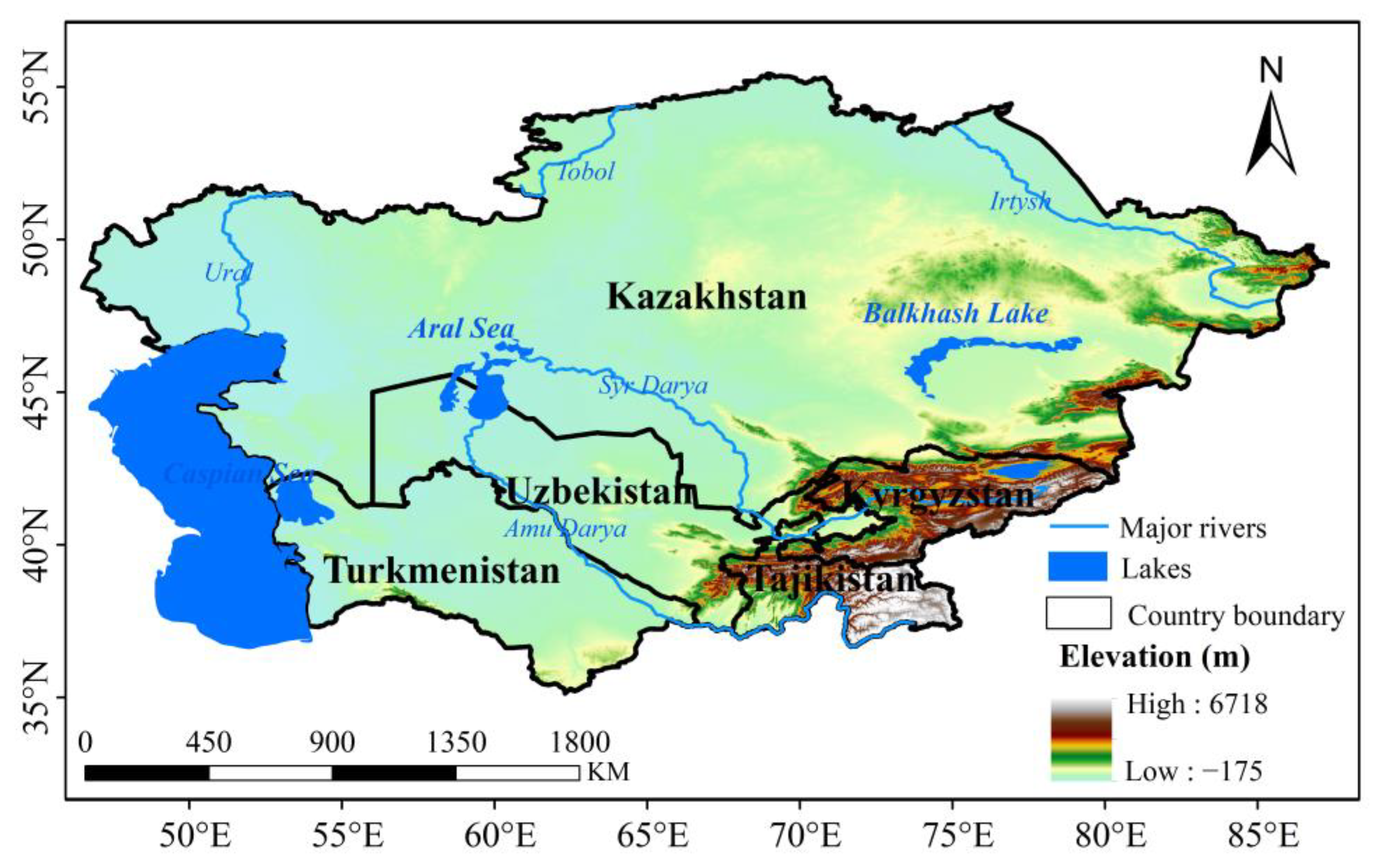
2.1. Study Area

With a total area of 566 × 104 km2, central Asia (CA) is situated between the latitudes of 30° 20′N and 50° 30′N and the longitudes of 46° 30′E and 96° 30′E (Figure 1). Kazakhstan (KAZ; 272.49 × 10⁴ km2), Kyrgyzstan (KGZ; 19.99 × 10⁴ km2), Tajikistan (TJK; 14.31 × 10⁴ km2), Turkmenistan (TKM; 49.12 × 10⁴ km2), and Uzbekistan (UZB; 44.74 × 10⁴ km2) are the five nations that make up CA. [21,22]. These states are present in the hinterlands of the Eurasian continent and have complex terrains and geomorphic features, including major lakes, rivers, and seas, such as Balkhash Lake, Issyk-Kul Lake, the Aral Sea, Syr River, and Amu River [23,24]. The study area of CA is known for its diverse geography and varying elevations and climates, which support a range of ecosystems and habitats. This region is also home to a rich cultural heritage, with ancient trade routes and Silk Road cities that have shaped its history and development. Studying this area is important for understanding the complex relationships between natural systems, human societies, and environmental changes. This has significant implications for water resource management, agriculture, biodiversity conservation, and sustainable development in the region.
In the five states of CA, the total water resources are mainly composed of surface water resources and groundwater resources [25]. The rich glacier resources are the major water resources for the terrestrial water storage components (e.g., rivers and lakes). The total terrestrial water storage of CA is about 1.877 × 10⁸ m3, which has uneven spatial distributions with the largest terrestrial water resources in KAZ, followed by TJK, KGZ, UZB, and TKM. The groundwater is mainly sourced from precipitation, snow water, and surface water. In the former Soviet republics, irrigation-intensive industries sucked water bodies dry in CA, which resulted in the serious Aral Sea crisis together with climate change [26].

2.2. Datasets

To investigate the variations in terrestrial water storage and their relationships with climate variables, in this study, we employed climate data and terrestrial water storage data sourced from multiple datasets (Table 1). In particular, the climate data include three variables, temperature (TMP), precipitation (PRE), and potential evapotranspiration (PET), which were obtained from the Climatic Research Unit (CRU) TS v4.06. The three climate variables have the same spatial resolution of 0.5° × 0.5°, covering the period of 1901–2020 [27]. In this study, the climate data were obtained from 2003 to 2020, which is consistent with the period of the terrestrial water storage and its components [28]. Analyzing long-term changes in TMP, PRE, and PET will help better understand the relationship between the water cycle and climate change. The performance of CRU datasets over CA has been evaluated in previous studies [29,30], and they have suggested that CRU datasets can effectively capture climatic variations and spatiotemporal characteristics in CA.
The terrestrial water storage components include SM, SWE, runoff, and groundwater. SM, SWE, and runoff datasets were downloaded from the Global Land Data Assimilation System (GLDAS) of NASA’s Earth Observing System Data and Information System (EOSDIS) Data Archive [28,29] with the same spatial resolution of 0.25° × 0.25°. The GLDAS uses advanced land surface modeling and data assimilation techniques to fuse satellite remote sensing observations and ground observations to generate the best fields that provide land surface states and fluxes [31,32,33]. The system drives multiple offline land surface models (e.g., Noah and Variable Infiltration Capacity (VIC) models) that integrate high-resolution data based on observations with global coverage. The GLDAS-2.0, GLDAS-2.1, 3-hourly, and monthly data products from the Noah land surface model (LSM) were divided into four layers (0–7, 7–28, 28–100, and 100–289 cm). The monthly GWSA products from the NOAH model simulations of GLDAS-2.0 GWSA (2003–2020) and GLDAS-2.1 GWSA (2000-present) were used in this study over a selected depth range of 0–10 cm, with a spatial resolution of 0.25° × 0.25°.
The TWSA data are derived from the Gravity Recovery and Climate Experiment (GRACE) products, which have been widely used to monitor the water storage and water fluxes in regional and global water resources analyses [34,35,36,37]. Launched in March 2002, the twin satellites known as GRACE analyze changes in the Earth’s gravitational field. Their data are used to examine changes in water supplies over land, ice, and oceans related to climate change and human activities [23]. Monthly fluctuations in the Earth’s gravity field over the basin can be used to detect vertically integrated changes in the water reserves of the planet. The monthly GRACE datasets are from April 2002 to present day, with spatial resolutions of 0.25° × 0.25°, 0.5° × 0.5°, and 1° × 1°. Generally, the TWSA data are derived from the Release dataset of the monthly GRACE Tellus products of the Centre for Space Research (CSR), the Geo Forschungs Zentrum (GFZ), the Jet Propulsion Laboratory (JPL), CSR GRACE Mascons and GRCTellus JPL-RL06 Mascons. Since June 2018, the Gravity Recovery and Climate Experiment Follow-On (GRACE-FO) has extended the 15-year monthly mass change record of the GRACE mission, which ended in June 2017. The GRACE-FO instrument and flight system performance improved over GRACE [38]. Extending the global mass change data record: GRACE Follow-On instrument and science data performance [39].
However, in this study, there is no observed record from meteorological station, hydrologic station, and groundwater well because it is very hard to obtain the observed record in CA.

2.3. Methods

In this study, before the comprehensive analysis of the terrestrial water cycle variations and their relationships with the three climate variables, the spatial resolutions of different variables are resampled using the bilinear interpolation method on the CRU dataset of 0.5° × 0.5°. The missing data of GRACE are filled using linear interpolation and monthly mean values. The record gap between the GRACE and GRACE-FO is filled by the convolutional neural network. Then, a continuous TWSA time series from the period of 2003 to 2020 is obtained as the study period.
The GWSA is derived from the TWSA, SM, and SWE according to the terrestrial water storage components and the water resource characteristics over CA as follows [16].
GWSA = TWSA − SMA − SWEA
where the SMA and SWEA are the SM anomaly and SWE anomaly based on the monthly mean value of the period of 2004–2009.
The linear trends of the climate factors, TWSA, and its components (i.e., SM, SWE, runoff, and GWSA) are computed using the linear least-squares method. The correlations between the climate factors and TWSA and its components are quantified by the correlation coefficient (CC). The significance of the linear trend and CC is examined at the 95% significant confidence level (p < 0.05). All the spatial and temporal variations are analyzed at annual and seasonal scales. The four seasons are defined as MAM (March, April, and May), JJA (June, July, and August), SON (September, October, and November), and DJF (December, January, and February).

3. Results

In this section, we present the spatiotemporal characteristics of the three climate variables (i.e., TMP, PRE, and PET) and four terrestrial water cycle components (i.e., SM, SWE, TWSA, and GWSA) from 2003 to 2020. For climatic variables, only the annual scale was considered. For SM, SWE, TWSA, and GWSA, both annual and seasonal scales were considered. A linear trend was used to illustrate the spatiotemporal variations in the hydro climatic variables, which were obtained using the linear least-squares method at a confidence level of 95% (p < 0.05).

3.1. Temporal and Spatial Characteristics of TMP, PRE, and PET

In this section, the temporal and spatial characteristics of the three climate variables, TMP, PRE, and PET, are explored using linear trends between 2003 and 2020. The annual variations in TMP, PRE, and PET provide the background of climate change for the terrestrial water cycle components.

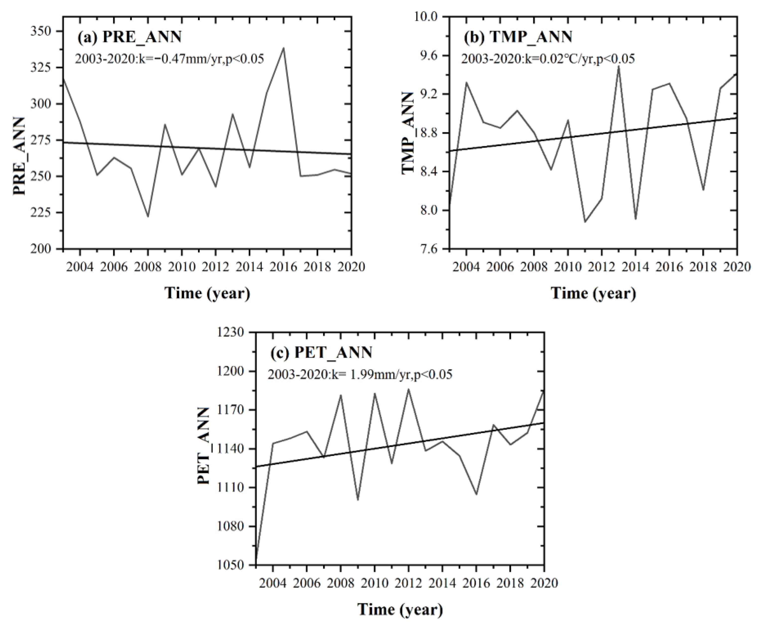
3.1.1. Temporal Characteristics of TMP, PRE, and PET

We observed a significant decreasing linear trend in the annual PRE, with a value of −0.46 mm/y (Figure 2a and Table 2). Large positive annual PRE anomalies were observed in 2003, 2009, 2013, and 2016, suggesting high PRE values during these years. Large negative anomalies in PRE were observed in 2005, 2008, 2010, 2012, 2014, and 2017, indicating lower PRE values during these years.
The annual PET showed a significant increasing linear trend in CA, with a value of 1.99 mm/yr over 18 years (p < 0.05). Positive TMP anomalies were observed in 2004, 2006, 2008, 2010, 2012, 2017, and 2020, indicating higher temperatures. Conversely, negative TMP anomalies were observed in 2003, 2009, 2011, 2014, and 2016, indicating cooler temperatures (Figure 2c).

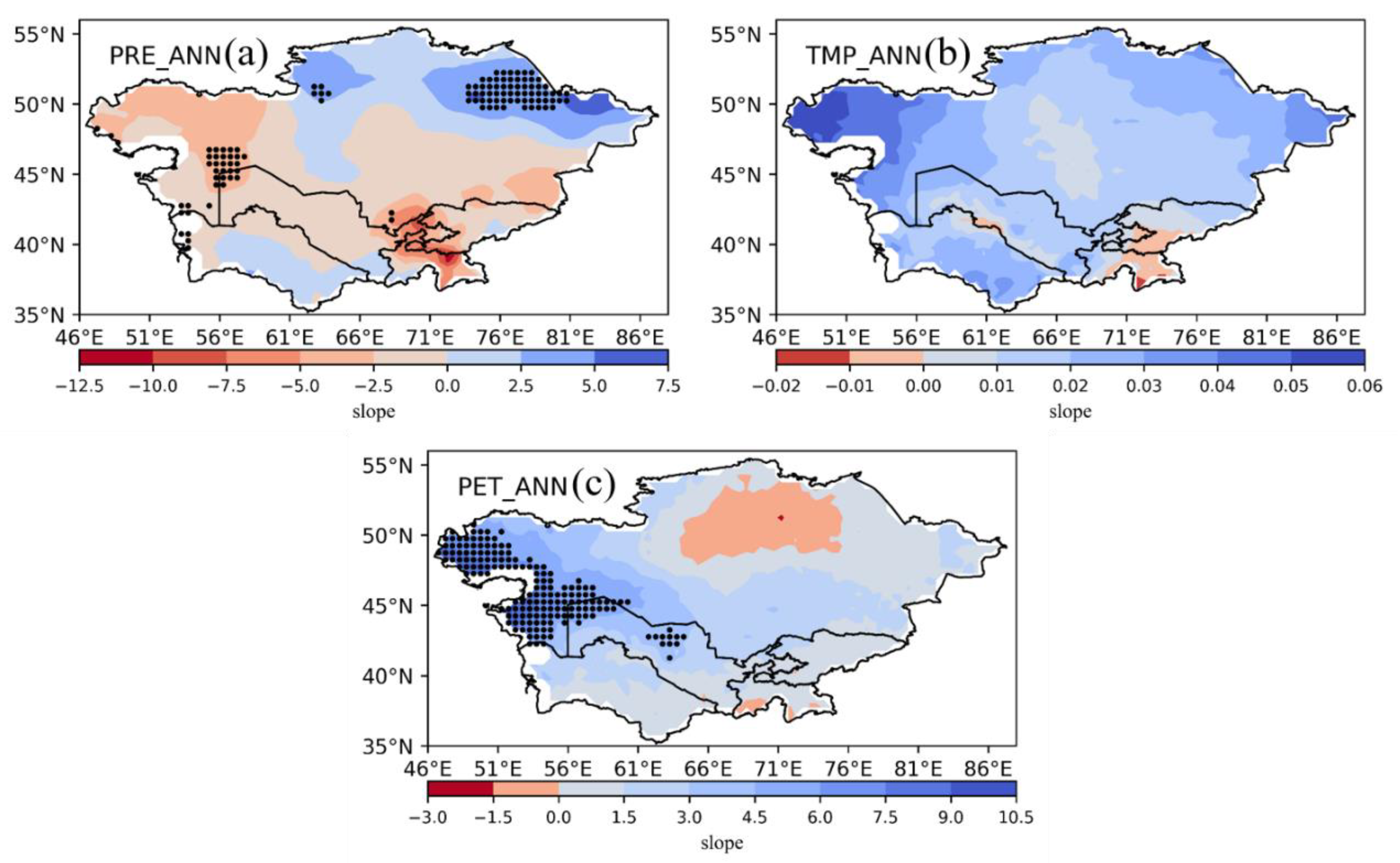
3.1.2. Spatial Characteristics of TMP, PRE, and PET

The spatial distributions of the linear trends of annual PRE, TMP, and PET are shown in Figure 3. The annual PRE and PET showed large spatial differences (Figure 3a,c). The annual TMP showed a consistently increasing linear trend over most of the study area.
In particular, the positive linear trends of the annual PRE were distributed over northern KAZ and most areas of TKM, with centers in the northeastern KAZ (Figure 3a). Parts of western KAZ and most areas of TJK and KGZ had decreasing centers. Moreover, positive linear trend areas accounted for 39% of the total, with a significant trend area of 4%. The negative linear trend areas of the annual PRE, as shown in Figure 3a, accounted for 61%, and the significantly negative trend areas accounted for 2%. The positive linear trends of the annual TMP were observed across most western areas of KAZ and TKM, wherein the centers were located in the western region of KAZ (Figure 3b). However, the southeastern parts of TJK and KGZ exhibited decreasing centers. Furthermore, areas displaying positive linear trends accounted for 97% of the total area, whereas those displaying negative trends accounted for only 3%, as shown in Figure 3b. As shown in Figure 3c, the positive linear trends of the annual PET are concentrated in western KAZ and northwestern UZB. Conversely, the northern and southern regions of KAZ and TJK, respectively, showed decreasing annual PET trends. Additionally, the significant trend areas accounted for 9% of the total area, with the remaining 88% showing a positive linear trend. Areas showing negative trends accounted for 12% of the total trend areas, as shown in Figure 3c.

3.2. Temporal and Spatial Characteristics of SM and SWE

In this section, we examine the temporal and spatial characteristics of two crucial climate variables, SM and SWE, by analyzing their linear trends between 2003 and 2020. We focused on the annual and seasonal variations in SM and SWE, which provide insights into components of the terrestrial water cycle. Exploring these variables can help obtain a better understanding of the changes in SM and SWE in CA.

3.2.1. Temporal Characteristics of SM and SWE

CA is a large and diverse region spanning several countries, including KAZ, UZB, TKM, TJK, and KGZ. The temporal characteristics of the SM in this region can vary depending on the specific location and local climate conditions. However, in some areas, the timing and amount of snowmelt are unpredictable, leading to fluctuations in SM levels. Overall, the annual and seasonal SM patterns in CA were influenced by the arid to semi-arid climate and topography of the region. Climate and land-use changes, such as increased irrigation and land degradation, can also have a significant impact on SM dynamics in the region.
Considering the annual and seasonal SWE, the temporal characteristics of SWE in CA varied depending on the specific location and elevation, as well as other factors, such as the weather patterns and topography. However, the annual SWE in CA is typically the highest in the winter months, with peak accumulation occurring in February or March. In spring, owing to temperature rise and the melting of snow, SWE begins to decrease. Seasonally, the SWE in CA varies depending on the region. For example, in the high-altitude regions of the Tian Shan and Pamir Mountains, the winter SWE accounts for more than 90% of the annual total, whereas in lower-elevation areas, such as the arid plains of KAZ, the SWE may be negligible or nonexistent. Notably, significant variability in SWE was observed from one year to another owing to weather patterns, and climate change is expected to have an impact on the timing and amount of SWE in CA in the following decades.

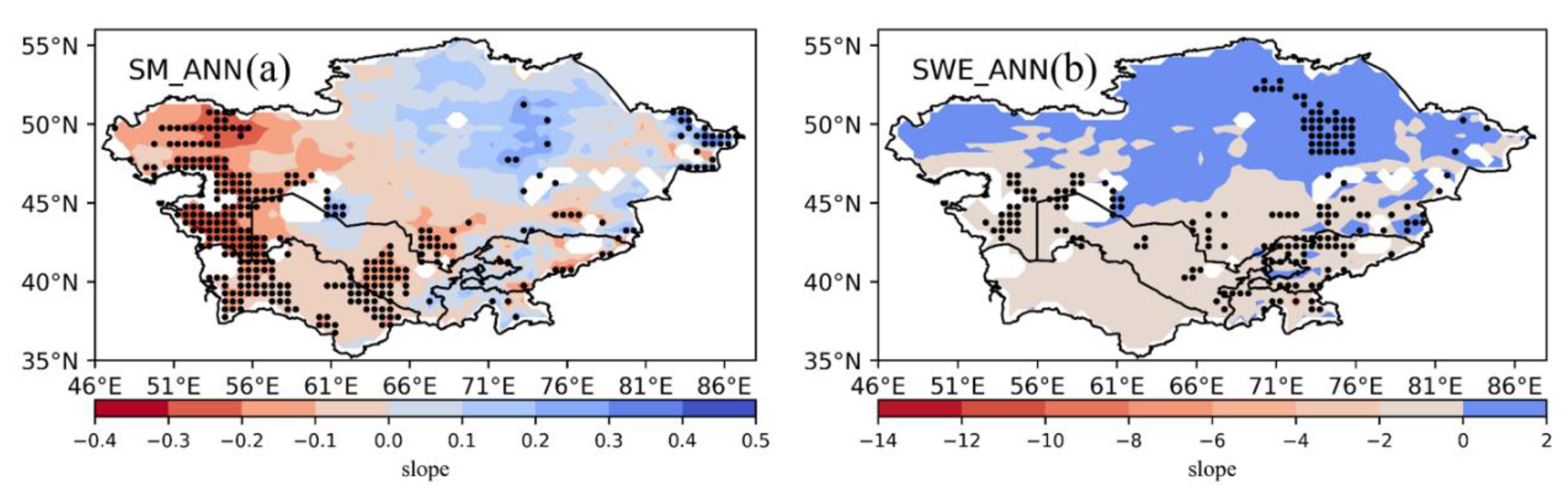
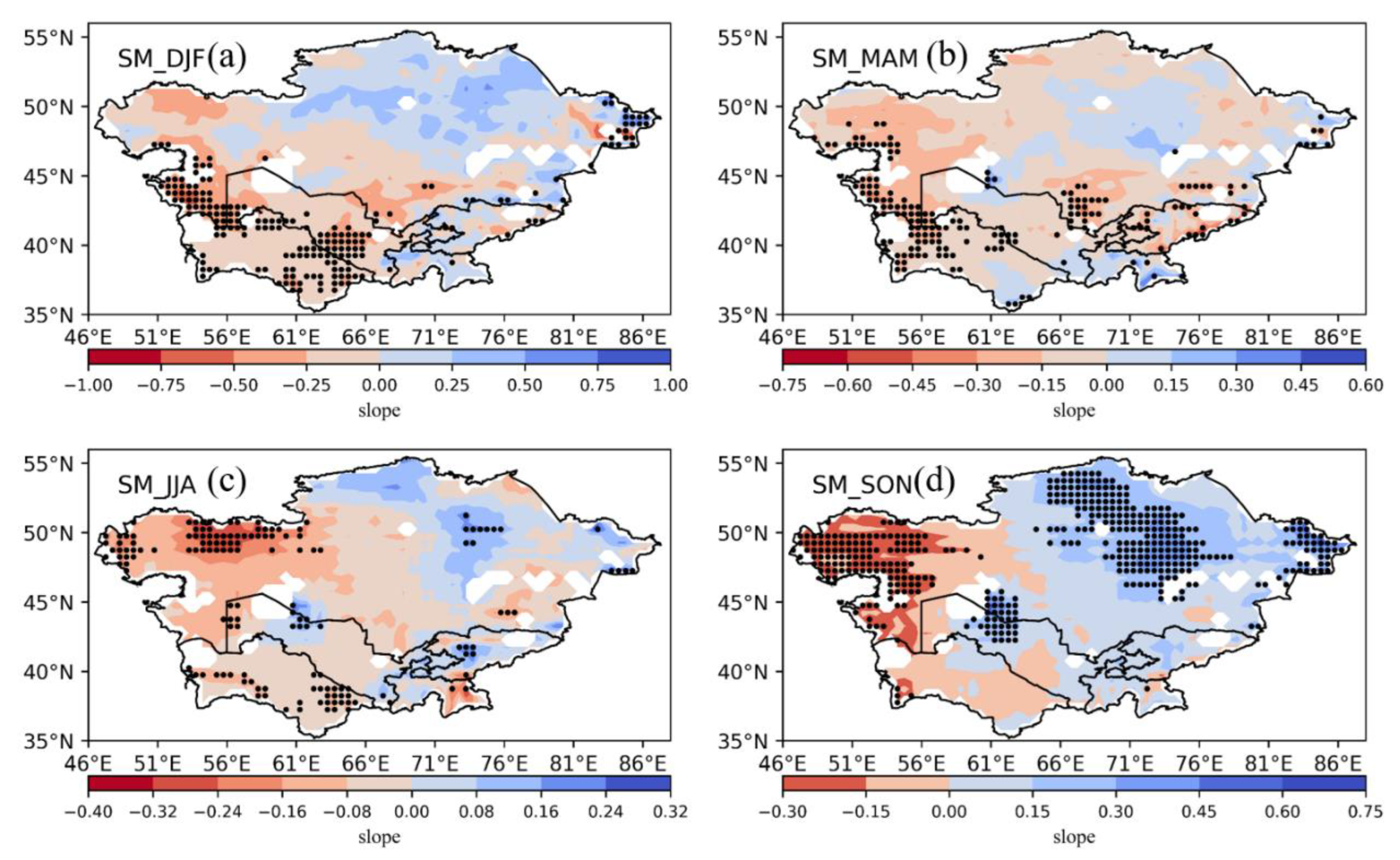
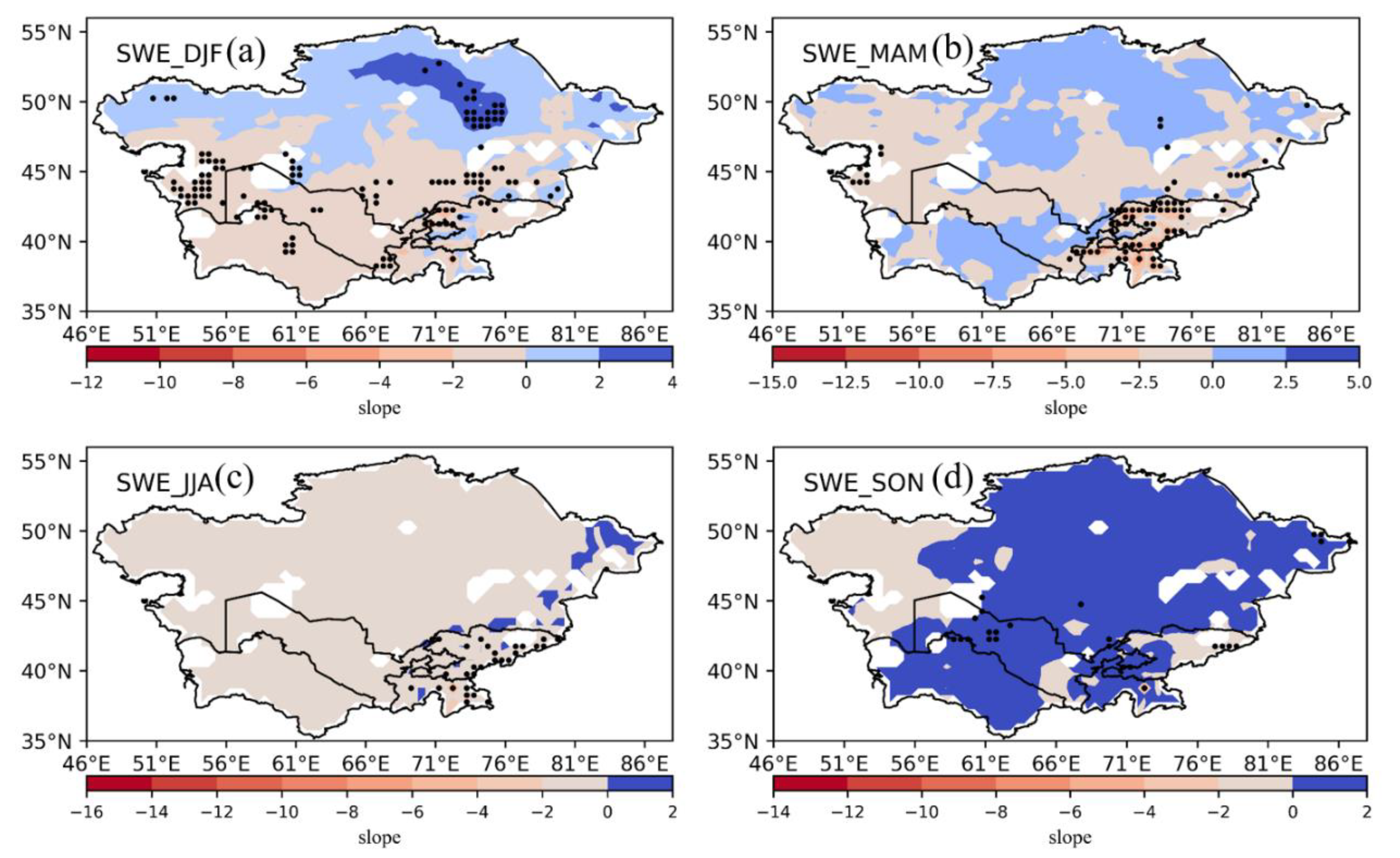
3.2.2. Spatial Characteristics of SM and SWE

Figure 4 depicts the spatial distributions of the linear trends obtained using the linear least-squares approach. To further analyze the data, we computed the percentages of areas with significantly increasing annual SM trends, as shown in Figure 5a. The results revealed that 42% of the areas exhibited a positive linear trend of annual SM of 3%. The areas showing significant increases in SM were mainly concentrated in KAZ, the western areas of TJK, and southwestern KGZ, whereas most of southwestern KAZ and southern TKM showed significantly decreasing SM trends. In particular, 16% of the areas demonstrated a negative linear trend in the annual SM, accounting for 58% of the total across the study area (Figure 4a).
The annual SWE was analyzed by determining the spatial distribution of linear trends using the linear least-squares approach. Additionally, the percentages of areas with significantly increasing annual SWE trends were calculated, as shown in Figure 5b. The findings indicated that 46% of the areas showed a positive linear trend of annual SWE of 4%. The areas showing significant increases in SWE were primarily concentrated in KAZ and the western, northern, and eastern regions of the study area. In contrast, the eastern TJK region shows a significantly decreasing trend of annual SWE. Notably, 7% of the areas exhibited a negative linear trend of annual SWE, accounting for 54% of the total across the study area (as shown in Figure 4b).
Figure 5 displays the spatial distributions of the linear trends of seasonal SM during the period of 2003–2020. DJF, MAM, and JJA have similar spatial distributions with the negative trends across most areas of CA (Figure 5a–c), and the significant decreased trends are distributed in western CA. The positive trends of the three seasons have the percentages of 42%, 26%, and 31% mainly distributed in parts of northern KAZ. The positive trend areas of SON SM are larger than the other seasons with the area shown in Figure 5. Moreover, the significant positive areas are mainly distributed across northern KAZ (Figure 5d), and the significant negative areas are distributed in northwestern KAZ with a percentage value of 17%.
The spatial distribution of linear trends of seasonal SWE was evaluated over 18 years from 2003 to 2020. Figure 6 shows the linear trends of seasonal SWE during MAM, JJA, SON, and DJF. Positive linear trends in seasonal SWE were observed over the northern and eastern regions of the study area, except for areas showing the greatest increase in SWE (Figure 6). These trends differ from the increasing trend observed for the annual SWE. During SON (Figure 6d), the SWE increased in most areas, but a significant drying trend was observed in KGZ, KAZ, TJK, UZB, and TKM. However, the northeastern and southeastern KAZ showed a significant increase in SWE of 78%. During JJA (Figure 6c), the SWE showed a significant increasing trend in the northeastern KAZ and southern TJK, whereas most areas showed a decreasing trend, except for southeastern TJK. Conversely, during MAM and DJF (Figure 6a,b), larger areas showed increasing trends than during DJF and SON. Regions showing increasing trends were mainly distributed in KAZ. We observed that the SWE in the western parts of the arid region of KGZ decreased slowly during spring, whereas it increased as a whole in autumn, wherein the speed of increase gradually decreased from northern KAZ to southern and eastern TJK.

3.3. Temporal and Spatial Characteristics of Runoff

In this section, we analyze the temporal and spatial characteristics of a crucial climate variable, runoff, by examining its linear trends from 2003 to 2020. We primarily focused on the annual and seasonal variations in runoff, which can provide valuable insights into the components of the terrestrial water cycle. The goal of this study was to gain a deeper understanding of changes in the runoff in CA.

3.3.1. Temporal Characteristics of Runoff

The annual runoff showed a significant negative linear trend, with a value of −0.0005 cm/a. Years with a positive anomaly in runoff occur 50% of the time, whereas those with negative anomalies comprise the remaining 50%. Among the four seasons, the greatest decreases in runoff were observed during JJA, MAM, DJF, and SON; these seasons showed significant negative linear trends of −0.0002, −0.0002, −0.0001, and 0.0003 cm/a, respectively.

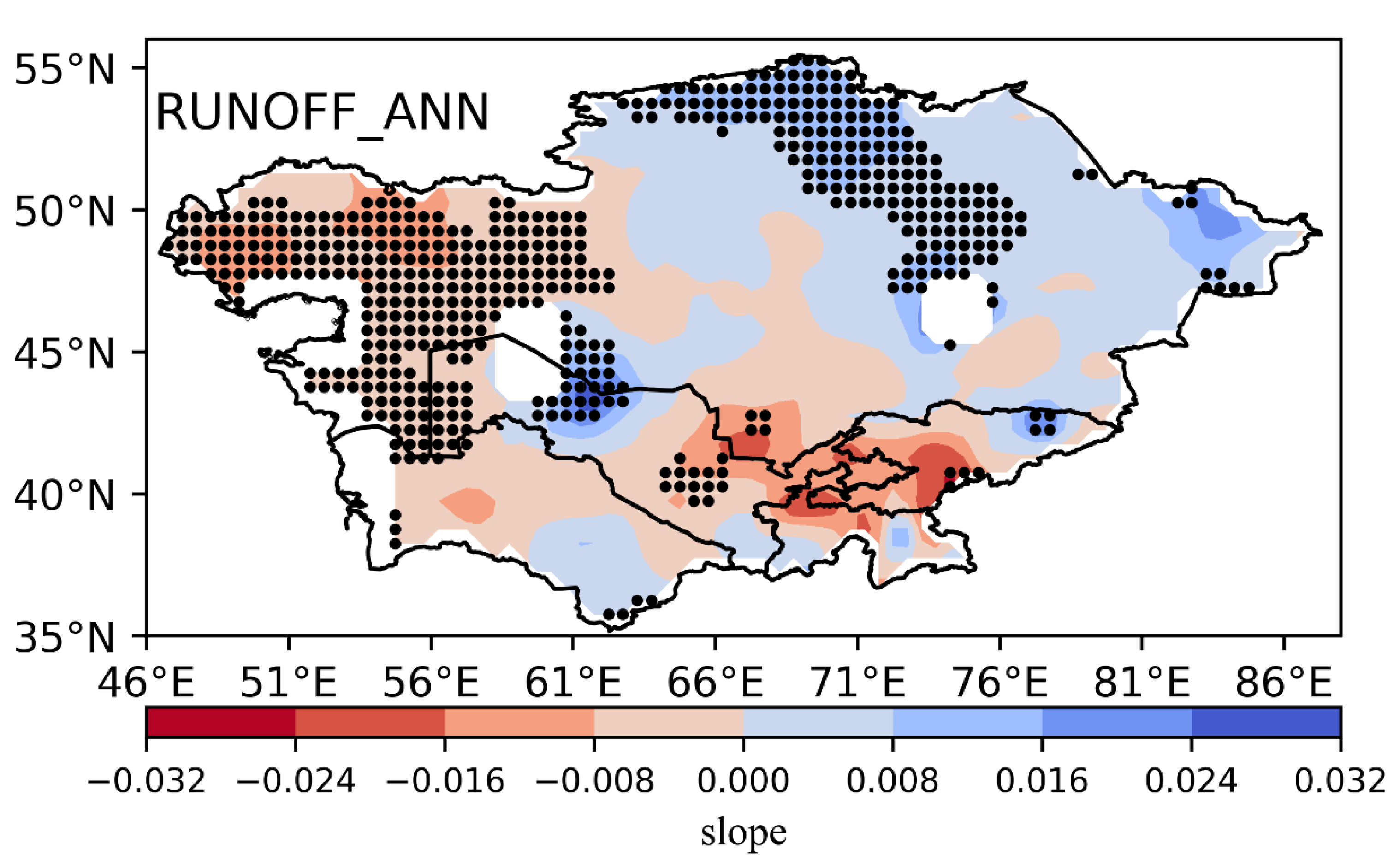
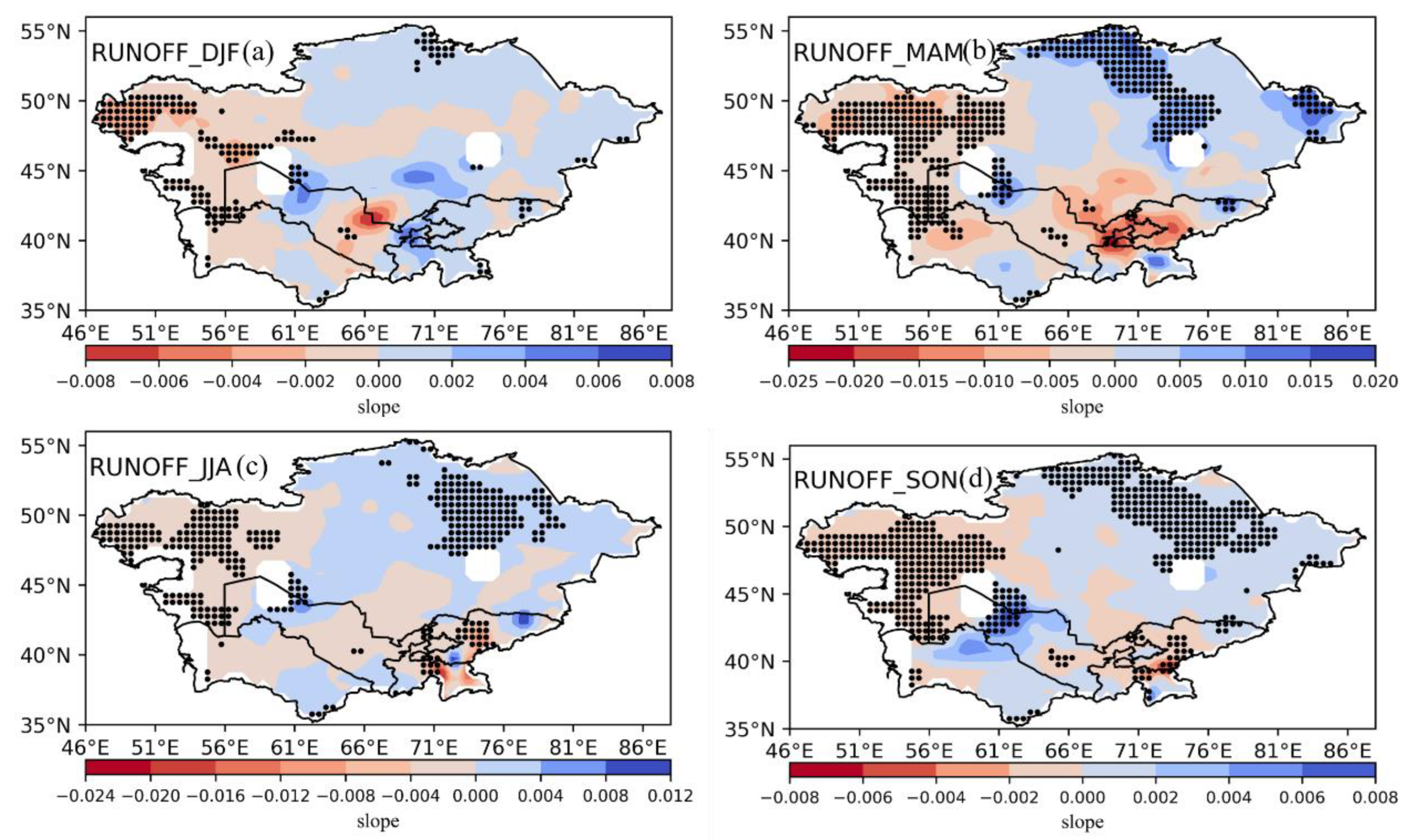
3.3.2. Spatial Characteristics of Runoff

In this section, we determine the spatial distribution of linear trends of the annual runoff. Our findings indicate that the positive linear trends are primarily distributed over the northeastern areas of KAZ, the northwestern parts of UZB, and the northeastern parts of KGZ, with centers in the northeastern part of the KAZ, as depicted in Figure 7. However, the northwestern parts of KAZ, including the region bordering northern TJK, the southeastern part, and a small portion of the northeastern parts of KGZ showed decreasing centers. Furthermore, areas showing positive linear trends accounted for 50% of the total, wherein areas showing significant trends accounted for 13%. In contrast, as shown in Figure 7, 50% of the areas showed negative linear trends, and areas showing significant negative trends accounted for 17%. Notably, areas showing negative trends were distributed over a more extensive region than those showing positive trends. Overall, the results suggest that the northeastern part of KAZ shows a positive annual runoff trend, whereas the northwestern parts of KAZ and some parts of KGZ show a negative annual runoff trend. However, further research is required to determine the underlying causes of these trends and their potential impacts on the region.
Figure 8 illustrates the spatial distribution of linear trends of seasonal runoff over 18 years from 2003 to 2020. Linear trends in seasonal runoff are shown for MAM, JJA, SON, and DJF. Negative linear trends in season runoff were observed in the southeastern regions of CA, except for areas with the greatest decrease in runoff (Figure 8). These trends differed from the decreasing trends of runoff during MAM (Figure 8b), wherein the runoff decreased in most areas, but a significant drying trend was observed in KGZ, TJK, KAZ, and UZB. However, the southeastern study area showed a significant decrease in runoff of 51%. During SON (Figure 8d), runoff showed a significant increasing trend in the southwestern areas of UZB and northern TKM. Although most areas showed a decreasing trend, there were exceptions in eastern TJK and southern KGZ. Conversely, during DJF and JJA (Figure 8a,b), larger areas showed increasing trends in northern TJK, eastern and northwestern UZB, and southern KAZ than during DJF. The regions with increasing trends were mainly distributed in KAZ and TJK. Runoff in the southern parts of the arid region of KAZ and northeastern UZB decreased slowly during winter, whereas it increased as a whole in autumn, wherein the rate of increase gradually decreased from KGZ to TJK.

3.4. Temporal and Spatial Characteristics of TWSA

In this section, we analyze the temporal and spatial characteristics of TWSA by examining its linear trends from 2003 to 2020. We focused on the annual and seasonal variations in the TWSA, which can provide valuable insights into the components of the terrestrial water cycle. Through this evaluation, we aimed to gain valuable insights regarding changes in the TWSA in CA.

3.4.1. Temporal Characteristics of TWSA

A significant negative linear trend was observed in the annual TWSA derived from JPL, with a value of −0.3065 cm/a. The percentage of positive anomaly years was 32%, and that of negative anomaly years was 68%. Among the four seasons, the largest decrease was observed in JJA, followed by MAM, DJF, and SON, with significant negative linear trends of −0.3483, −0.3291, −0.2917, and −0.2464 cm/a.

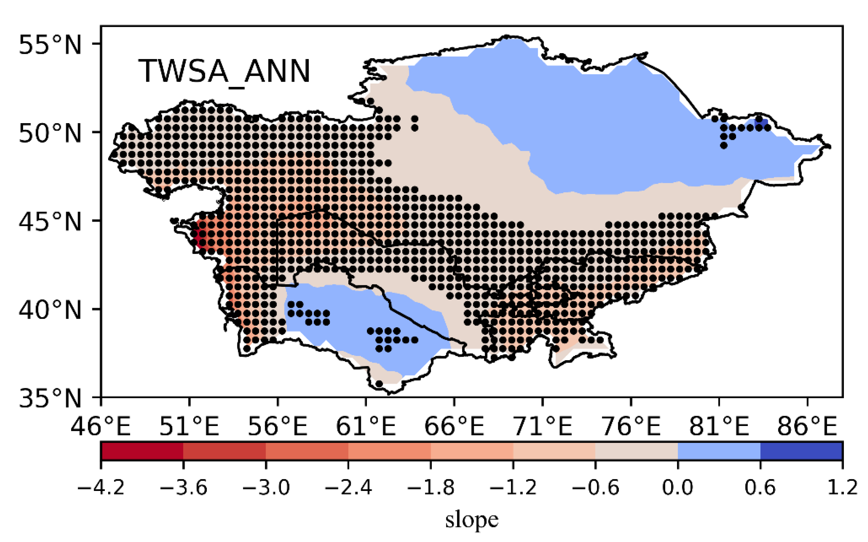
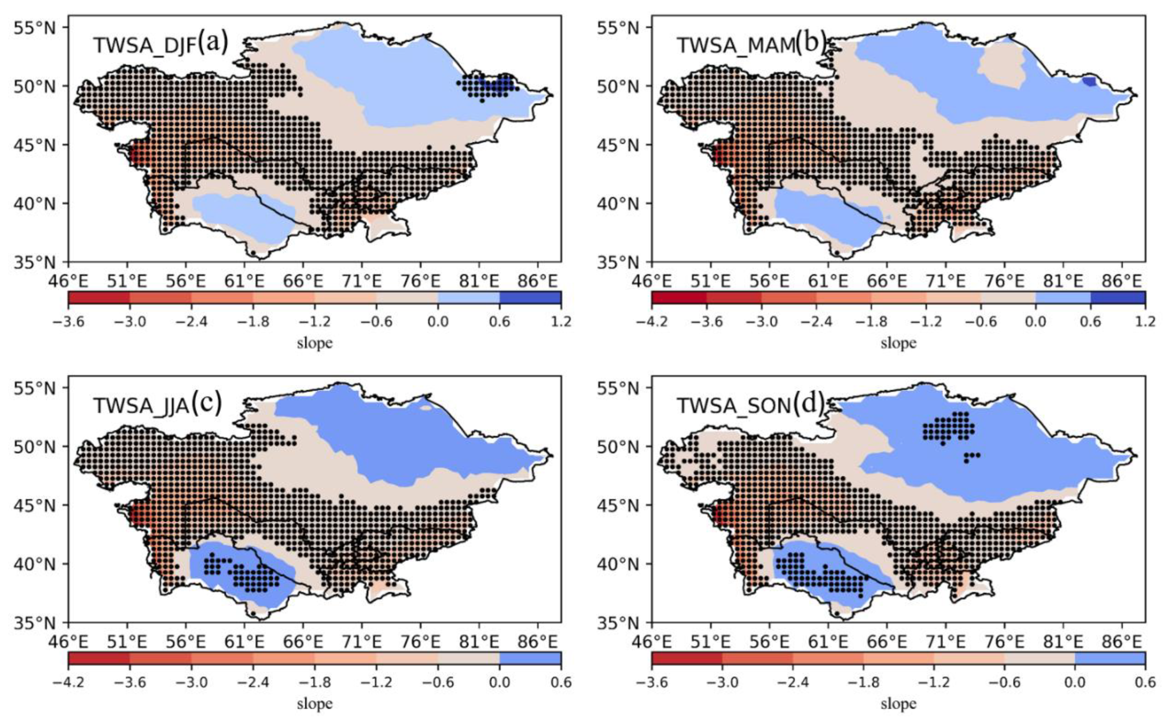
3.4.2. Spatial Characteristics of TWSA

In this section, we analyze the annual TWSA and determine the spatial distribution of linear trends. Positive linear trends were distributed over northeastern KAZ and most areas of TKM, wherein the centers were observed in the northeastern part of KAZ, as depicted in Figure 9. However, southwestern KAZ and short western TKM showed decreasing centers. Additionally, areas showing positive linear trends accounted for 32% of the total, wherein areas showing significant trends accounted for 2%. In contrast, as shown in Figure 9, areas showing negative linear trends accounted for 68%, and those showing significantly negative trends accounted for 49%.
Figure 10 shows the spatial distribution of linear trends in the surface TWSA during the vegetation period from 2003 to 2020 for four seasons: MAM, JJA, SON, and DJF. Positive linear trends in the TWSA during the growing season were observed in the northern and eastern regions of the study area, except for areas with the most decreased TKM TWSA (Figure 10b). These trends differ from the decreasing trend observed in the annual TWSA (Figure 9). For instance, during MAM (Figure 10b), the TWSA decreased in most areas, and a significant drying trend was observed in KGZ and KAZ. However, southwestern KAZ, northwestern TKM, and eastern TJK experienced a significant decrease in TWSA of 47%, but positive trends were observed in northeastern KAZ (with a value of 27%). During JJA (Figure 10c), the TWSA showed a significant increasing trend in northwestern KAZ, central TKM, and southern UZB, whereas most areas showed a decreasing trend, except for southwestern KAZ and western TKM. Conversely, during SON and DJF (Figure 10a,d), larger areas showed decreasing trends than during MAM and JJA. The regions showing increasing trends were mainly distributed in KAZ and TKM. We observed that the TWSA in the southwestern parts of the arid region of KAZ decreased slowly during spring, whereas it increased as a whole in autumn, wherein the increasing speed gradually decreased from northeastern KAZ to southern and eastern TJK and TKM.

3.5. Temporal and Spatial Characteristics of GWSA

CA is an arid region with limited water resources, and groundwater is a vital source of water for agricultural, industrial, and domestic use. A study on the temporal and spatial characteristics of GWSA from 2003 to 2020 in CA found that the region has experienced significant changes in groundwater levels over the years. Furthermore, the study revealed that GWSA mainly occurred in the eastern part of CA, particularly in the Tarim and Amu Darya basins. This anomaly is characterized by a persistent decline in groundwater levels, indicating the unsustainable use of terrestrial water cycle components in these regions. In this section, we analyzed the temporal and spatial characteristics of the GWSA during 2003–2020, both at annual and seasonal scales.

3.5.1. Temporal Characteristics of GWSA

A significant negative linear trend was observed in GWSA derived from the JPL and GLDAS, with a value of −0.2742 cm/a. The percentage of positive anomaly years was 32%, and that of negative anomaly years was 68%. Among the four seasons, the largest decrease was observed in JJA, followed by DJF, MAM, and SON, with significant negative linear trends of −0.3033, −0.2796, −0.2748, and −0.2222 cm/a.

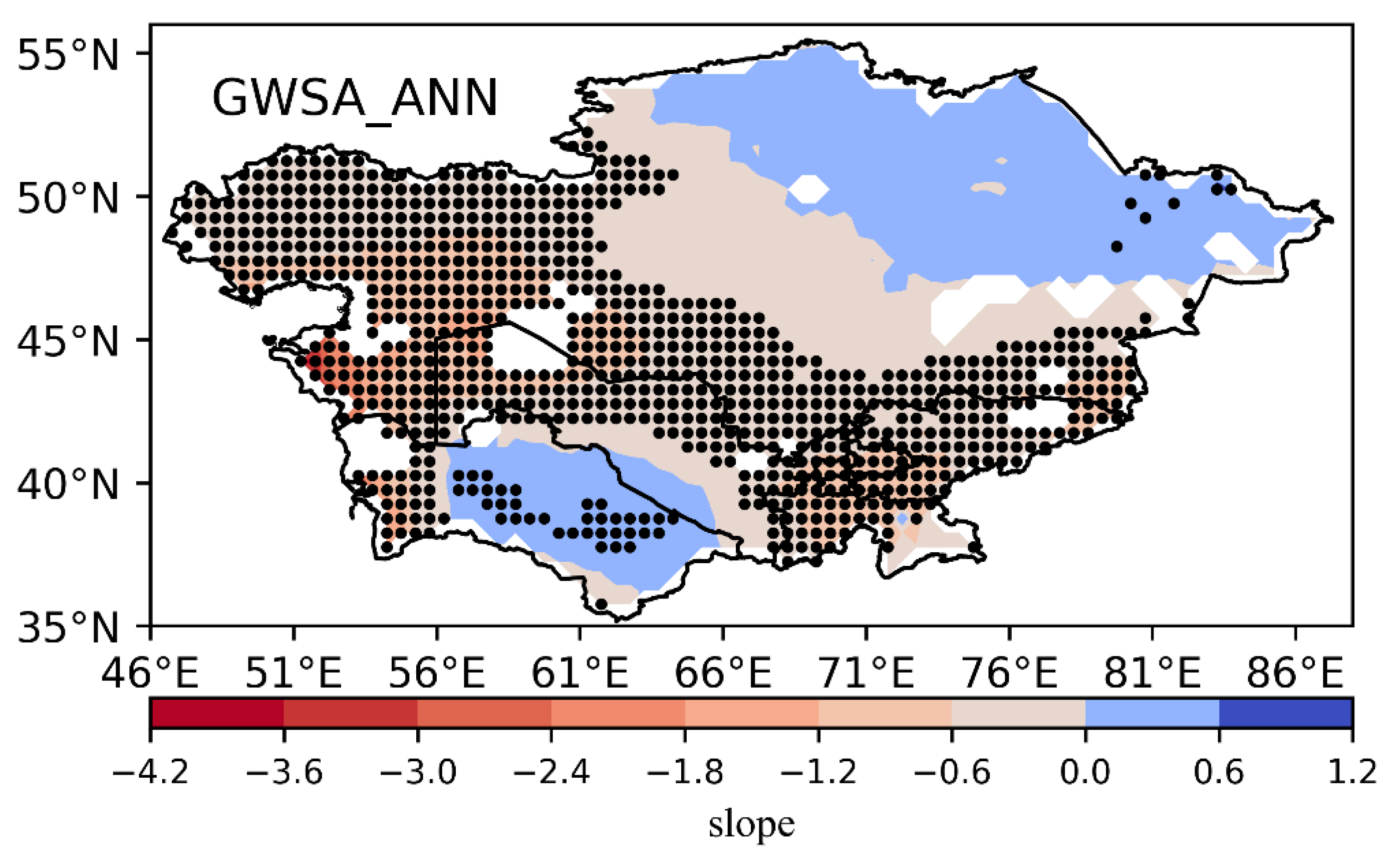
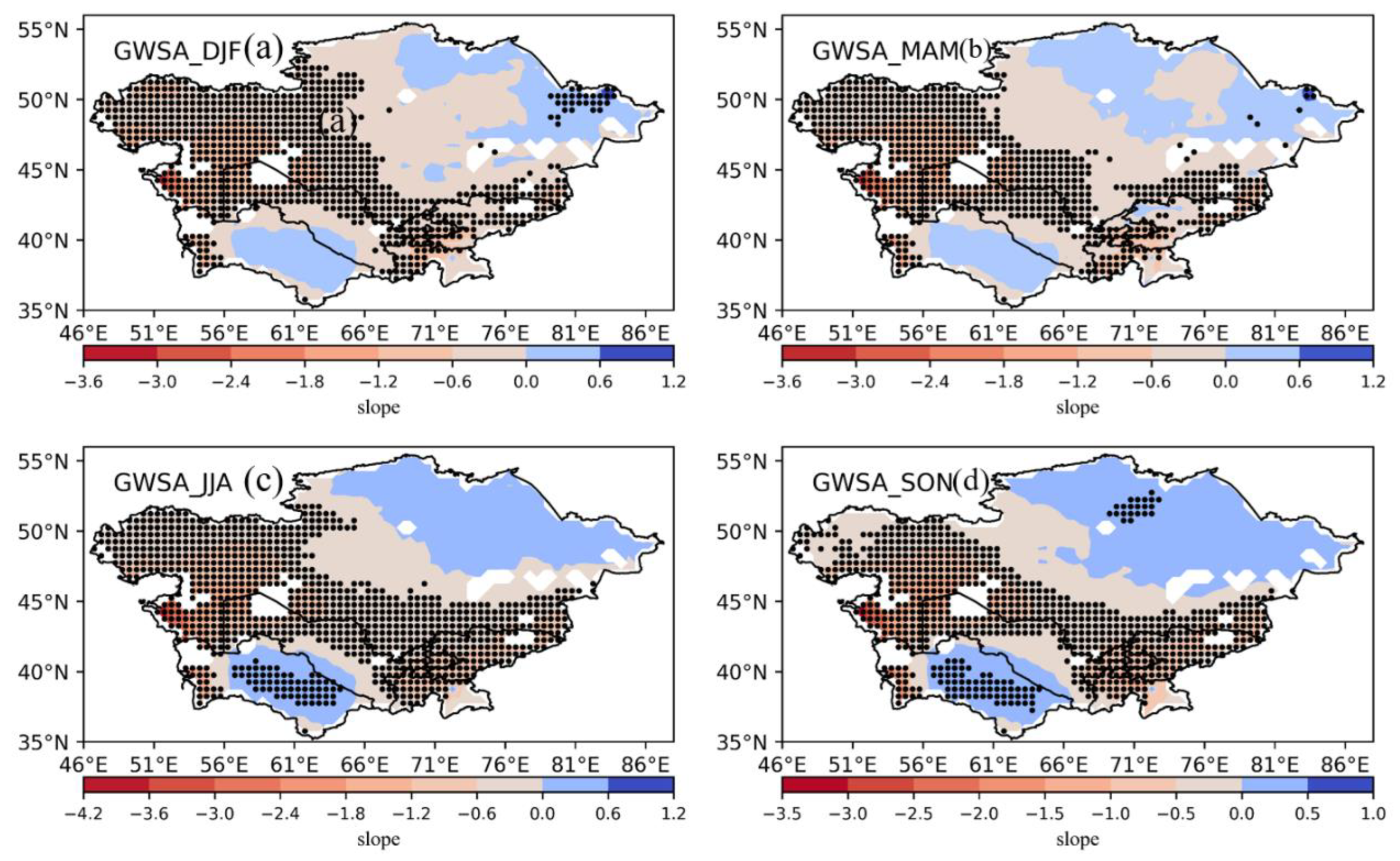
3.5.2. Spatial Characteristics of GWSA

Approximately 47% of the areas in CA showed significant negative trends for the annual GWSA, and approximately 3% showed significant positive trends (Figure 11). The trends in other areas were insignificant. The spatial distributions of the linear trends in GWSA were very similar, with negative centers of 68% in southwestern KAZ, central TJK, southwestern KGZ, and western TKM. Positive centers were observed in northeastern KAZ, northeastern TKM, and southeastern UZB (32%) (Figure 11). Most areas in CA showed decreasing trends for GWSA.
Compared with the annual GWSA, the areas with significant trends in the seasonal GWSA in JJA were smaller, especially for areas with significant negative trends of 48% (Figure 12c). The negative centers in parts of southwestern KAZ and western TKM show decreasing trends in seasonal GWSA, and positive centers showing increasing linear trends in seasonal GWSA during JJA still appear in the same regions as the annual GWSA. During MAM, most areas of KAZ, western–southern TKM, and western and eastern TJK showed insignificant changes of 41%, as shown in Figure 12b. During the other two seasons, areas showing significant positive/negative trends in GWSA were equivalent to those during SON and DJF (Figure 12a,d). The areas showing significant positive trends during SON and JJA were larger than those during SON and DJF.

4. Discussion

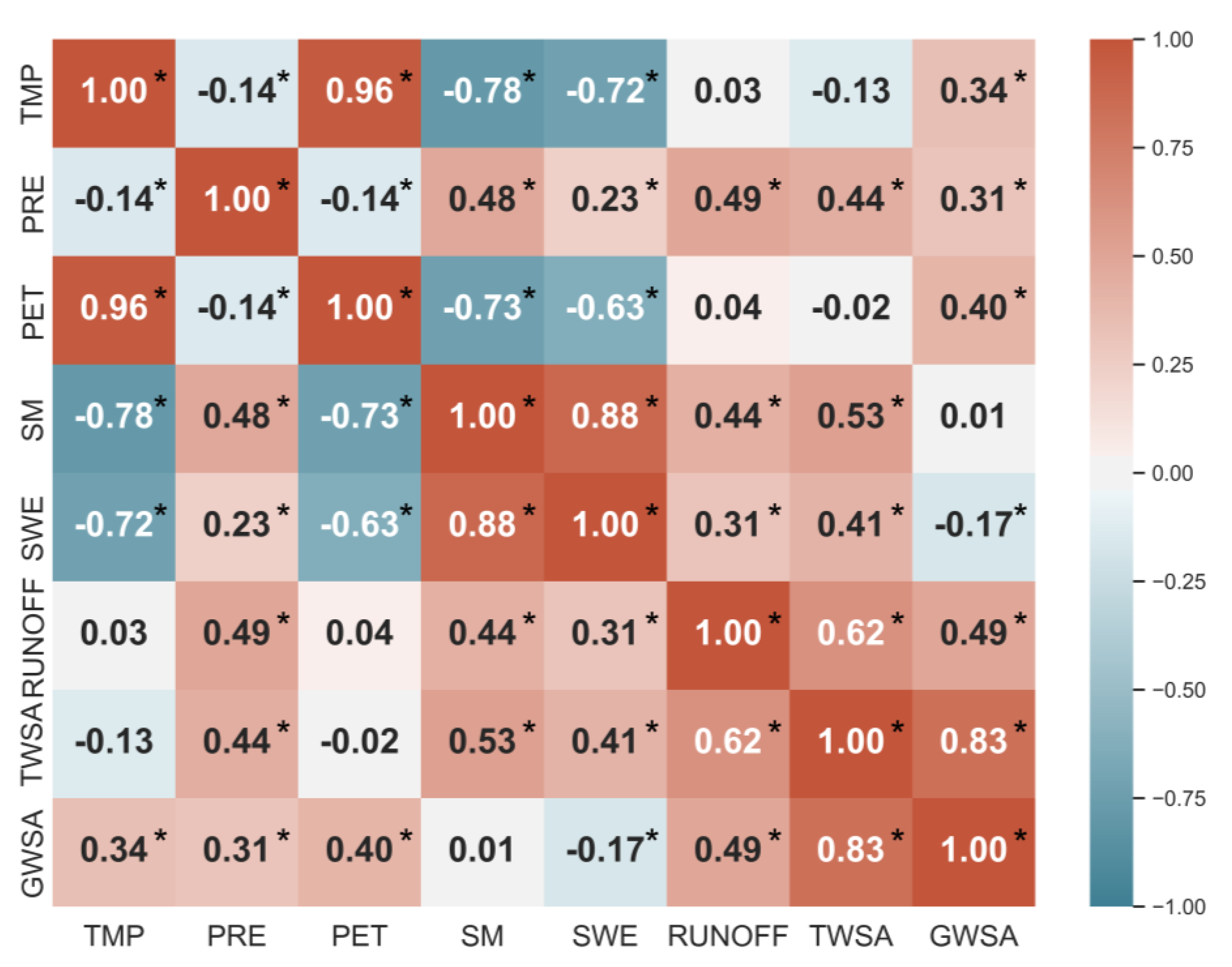
4.1. Relationships between the Climate Variables and the Different Terrestrial Water Components

The terrestrial water cycle components of CA are complex [1,14], and the relationships between the different components need to be clarified [21]. Based on a previous study, we evaluated the impacts of PRE and TMP on various hydrological variables, such as TWSA, TMP, PRE, PET, SM, SWE, RUNOFF, and GWSA. The study found that PRE had positive impacts on terrestrial water cycle components, as indicated by the similar variations between the CCs of the two variables shown in Figure 13. Additionally, increased CCs were observed between the TWSA and several other variables, including PET and GWSA, when compared with that between TMP and other variables. However, TMP negatively impacted several other hydrological variables, such as PRE, SM, SWE, and TWSA, as indicated by the negative CCs. In particular, the CCs between TMP and PRE, SM, SWE, TWSA, and GWSA are −0.14 *, −0.78 *, −0.72 *, −0.13, and −0.17 *, respectively. Overall, PRE was found to have a positive impact on the TWSA and other hydrological variables, whereas TMP has negative impacts on some of these variables. Notably, these findings may depend on the specific location and periods studied as well as the methods used for analysis.

4.2. Water Resources and Water Withdrawal over Central Asia during 1999–2019

This section presents a comprehensive analysis of the rising water demand and decreasing terrestrial water cycle components, which are closely related to sustainable development goal (SDG) 6.4.2, related to the water and water management strategies in CA. According to SDG 6.4.2, the level of water stress is freshwater extraction as a share of available freshwater resources; this represents the ratio between the total freshwater extraction of the main sectors of the economy and the total renewable freshwater resources, considering the water requirements of the environment (https://www.fao.org/sustainable-development-goals/data/en, accessed on 21 December 2022).
The variability in cultivated areas (arable land and permanent crops) significantly impacts water consumption and abstraction, particularly in dry regions. This section analyzes the variation in the crop area of five countries (KAZ, KGZ, TJK, TKM, and UZB) in CA to illustrate the change in water resources in the dry regions of CA.
The cultivated area of KAZ decreased from 3220 × 104 ha in 1999 to 2999 × 104 ha in 2019 at a rate of 10.5 × 10⁴ ha/year, representing a decrease of 0.99%. Considering UZB, the sown area decreased from 483 × 104 ha in 1999 to 475 × 104 ha in 2009 and then increased to 444 × 104 ha in 2019. The sown area of KGZ decreased from 14.3 × 10⁴ ha in 1999 to 13.64 × 10⁴ ha in 2019. The sown area slightly decreased from 88.6 × 10⁴ ha in 1999 to 85.3 × 10⁴ ha in 2019 in TJK. In TKM, the sown area increased from 189 × 104 ha in 1999 and 2004 to 205 × 104 ha in 2014 and 2019 (Table 3). This indicates that KAZ had the largest cultivation area, followed by UZB and TKM. Considering the irrigated area, KAZ had a very small percentage of cultivated area, and the cultivated areas of the other four countries almost accounted for the remaining irrigated area. For example, UZB had the largest irrigated area of 456 × 104 ha in 2009, followed by KAZ (2874 × 104 ha) and TKM (205 × 104 ha). TJK has the smallest irrigated area, with a value of 88.4 × 10⁴ ha in 2009.
For each of the three water resource variables, each country had the same value in five years, namely, 1999, 2004, 2009, 2014, and 2019, indicating that the renewable water resources of the five countries did not change during 1999–2019 (Table 3). Significant differences were observed in renewable water resources among the five countries. In particular, KAZ has the largest total renewable water resources, total renewable surface water, and total renewable groundwater, with values of 108.4, 100.6, and 33.85 Gt/y during 1999–2019, respectively. The total renewable water resources, total renewable surface water, and total renewable groundwater in CA were 227.57, 207.09, and 62.745 Gt/y, respectively. However, the total renewable groundwater in CA is vulnerable and sensitive, with a small share of total renewable water resources (i.e., 227.57, 207.09, and 62.745 Gt/y, with percentages of 5.8, 6.4, and 21%, respectively). These results were consistent with the water stress values for CA from SDG 6.4.2 (Table 3). Moreover, comparing the annual TWSA of reservoir depletion, the decrease in the annual TWSA was 5.8% of the total renewable water resources for CA at the current rate of depletion, indicating that renewable water supplies in some states may have been depleted in 1999. During 1999–2019, in UZB and TKM, the water used during the total withdrawal (i.e., 59.8 Gt/y in 1999 and 57.1 Gt/y in 2005 for UZB; 27.95 Gt/y in 2004 and 27.95 Gt/y in 2009 for TKM) and water extraction for agriculture (i.e., 54.1 Gt/y in 2009 and 51.8 Gt/y in 2014 for UZB; 27.95 Gt/y in 2014 and 27.95 Gt/y in 2019 for TKM) was greater than that in KAZ, KGZ, and TJBK. In terms of water use in different years, the total water withdrawal rates of KAZ and TKM increased from 23.5 Gt/y (1999) to 25 Gt/y (2019) and 24.91 Gt/y (1999) to 27.95 Gt/y (2019), respectively. In other countries, the total water withdrawal decreased due to a decrease in the cultivated area. Except for TJK, all the other countries have seen a decline in agricultural water use based on agricultural water withdrawal rates. Moreover, the percentage of water extraction for agricultural use regarding total water withdrawal is declining, mainly due to the decrease in cultivated areas, especially in CA, with a percentage decrease from 10% in 1999 to 9% in 2019. This also shows that water extraction for agricultural use in CA accounted for nearly all water extraction activities (over 10% in CA). Regarding the relationship between annual water depletion in terms of the TWSA and total water withdrawal, total water withdrawal in CA has little effect on the decrease in TWSA (e.g., 10% in 1999 vs. 10% in 2019). Finally, the value of water stress variables (%) in CA decreased from 2.9% in 1999 to 2.8% in 2019 and from 3% in 2009 to 2.9% in 2004, indicating the severity of water scarcity in CA. Reduced water stress has also been observed in CA. Compared with that in other countries, water stress appears to be higher in TJK and UZB, which is consistent with their higher levels of water storage (Table 3). Moreover, a water load of more than 100% in TKM and UZB indicates that the total renewable freshwater resources cannot meet the socioeconomic demand for water, which may lead to the over-exploration of groundwater.

5. Conclusions

In this study, the temporal and spatial characteristics of the terrestrial water cycle and their relationships with the climate variables across CA are comprehensively analyzed at annual and seasonal scales during the two decades of 2003–2020. The major results are as follows:
For TWSA and GWSA, they have significant decreasing trends at annual and seasonal scales with annual linear trend values of −0.31 and −0.27 cm/a, respectively, which indicate large water depletion during the period of 2003–2020. For the seasonal changes, the largest water depletions are observed in JJA with linear trend values of −0.35 and −0.30 cm/a for TWSA and GWSA. Moreover, the depletion centers were spatially distributed over most areas of western and southern KAZ and nearly all areas of UZB, KGZ, and TJK.
For SM, SWE, and runoff, except for the increased SM during SON, SM showed a decreasing trend at annual and seasonal scales. The annual, SON, and DJF values of SWE showed increasing trends. Weak linear trends in runoff were observed at annual and seasonal scales.
The increased TMP and PET and the decreased PRE have significant impacts on the terrestrial water cycle in CA. Particularly, TMP and PET had the largest significant negative impacts on SM and SWE compared with the other terrestrial water components. PRE had a positive impact on terrestrial water variations, with similar impacts on SM (CC = 0.48), runoff (CC = 0.49), and TWSA (CC = 0.44). SM, SWE, runoff, and GWSA had significant positive contributions to the variations in TWSA. GWSA had the largest contribution, followed by runoff, SM, and SWE.
Considering water resources and water withdrawal in CA during 1999–2019, water withdrawal did not significantly increase, whereas terrestrial water storage experienced a significant decreasing trend. This suggests that the large depletion of water resources in CA may be mainly caused by climate change. Therefore, according to our analysis, the water resource depletion in CA has been primarily caused by climate change in the last two decades (2003–2020). The differences in the spatial distributions of TWS result in different water resource challenges. Our results provide a comprehensive understanding of terrestrial water resource variation that plays a significant role in water resource management and the SDG in CA.

Author Contributions

Conceptualization, M.O., Z.H. and X.C.; data curation, X.C., Z.Z., H.Z. and M.W.; formal analysis, M.O., Z.H. and M.M.; funding acquisition, X.C.; investigation, H.Z.; methodology, M.O., Z.H., X.C., M.M., Z.Z. and M.W.; project administration, X.C.; resources, Z.H. and M.M.; software, M.O., M.M. and Z.Z.; supervision, X.C.; validation, M.O. and Z.Z.; visualization, M.O., Z.H., M.M. and H.Z.; writing—original draft, M.O.; writing—review and editing, Z.H. All authors have read and agreed to the published version of the manuscript.

Funding

This study was supported by the National Natural Science Foundation of China, grant number 42230708, 41971386, Western Scholars of the Chinese Academy of Sciences, grant number 2020-XBQNXZ-010, the National Youth Talent Project, grant number E1190301 and the Third Xinjiang Scientific Expedition Program, grant number 2021xjkk1300.

Data Availability Statement

GRACE data are from https://grace.jpl.nasa.gov/data/get-data/ (accessed on 21 December 2022). GLDAS 2.1 were downloaded from https://disc.gsfc.nasa.gov/datasets?keywords=GLDAS (accessed on 21 December 2022). TMP, PRE, and PET were found from CRU TS v 4.01 from CRU TS v 4.06 https://crudata.uea.ac.uk/cru/data/hrg/ (accessed on 21 December 2022). Monthly surface climate China V2.0 was downloaded from http://data.cma.cn/ (accessed on 21 December 2022).

Acknowledgments

This study is the part of Ph.D. research of Mirshakar Odinaev and has been sponsored by the CAS-TWAS President’s Fellowship for International Ph.D. Students awarded to him.

Conflicts of Interest

The authors declare no conflict of interest.

References

  1. Hu, Z.; Chen, X.; Zhou, Q.; Yin, G.; Liu, J. Dynamical variations of the terrestrial water cycle components and the influences of the climate factors over the Aral Sea Basin through multiple datasets. J. Hydrol. 2022, 604, 127270. [Google Scholar] [CrossRef]
  2. Chen, J.; Famigliett, J.S.; Scanlon, B.R.; Rodell, M. Groundwater storage changes: Present status from GRACE observations. In Remote Sensing and Water Resources. Space Sciences Series of ISSI; Springer: Cham, Switzerland, 2016; pp. 207–227. [Google Scholar]
  3. McColl, K.A.; Roderick, M.L.; Berg, A.; Scheff, J. The terrestrial water cycle in a warming world. Nat. Clim. Change 2022, 12, 604–606. [Google Scholar] [CrossRef]
  4. Hu, Z.; Zhou, Q.; Chen, X.; Qian, C.; Wang, S.; Li, J. Variations and changes of annual precipitation in Central Asia over the last century. Int. J. Climatol. 2017, 37, 157–170. [Google Scholar] [CrossRef]
  5. Yin, D.; Roderick, M.L. Inter-annual variability of the global terrestrial water cycle. Hydrol. Earth Syst. Sci. 2020, 24, 381–396. [Google Scholar] [CrossRef] [Green Version]
  6. Zhou, Q.; Huang, J.; Hu, Z.; Yin, G. Spatial-temporal changes to GRACE-derived terrestrial water storage in response to climate change in arid Northwest China. Hydrol. Sci. J. 2022, 67, 535–549. [Google Scholar] [CrossRef]
  7. Kåresdotter, E.; Destouni, G.; Ghajarnia, N.; Lammers, R.B.; Kalantari, Z. Distinguishing Direct Human-Driven Effects on the Global Terrestrial Water Cycle. Earth’s Future 2022, 10, e2022EF002848. [Google Scholar] [CrossRef]
  8. Rummler, T.; Arnault, J.; Gochis, D.; Kunstmann, H. Role of lateral terrestrial water flow on the regional water cycle in a complex terrain region: Investigation with a fully coupled model system. J. Geophys. Res. Atmos. 2019, 124, 507–529. [Google Scholar] [CrossRef]
  9. Lv, M.; Ma, Z.; Peng, S. Responses of terrestrial water cycle components to afforestation within and around the Yellow River basin. Atmos. Ocean. Sci. Lett. 2019, 12, 116–123. [Google Scholar] [CrossRef] [Green Version]
  10. Harding, R.; Best, M.; Blyth, E.; Hagemann, S.; Kabat, P.; Tallaksen, L.M.; Warnaars, T.; Wiberg, D.; Weedon, G.P.; Lanen, H.V. WATCH: Current knowledge of the terrestrial global water cycle. J. Hydrometeorol. 2011, 12, 1149–1156. [Google Scholar] [CrossRef]
  11. Yang, W.; Yang, H.; Li, C.; Wang, T.; Liu, Z.; Hu, Q.; Yang, D. Long-term reconstruction of satellite-based precipitation, soil moisture, and snow water equivalent in China. Hydrol. Earth Syst. Sci. 2022, 26, 6427–6441. [Google Scholar] [CrossRef]
  12. Hu, Z.; Chen, X.; Li, Y.; Zhou, Q.; Yin, G. Temporal and Spatial variations of soil moisture over Xinjiang based on multiple GLDAS datasets. Front. Earth Sci. 2021, 9, 654848. [Google Scholar] [CrossRef]
  13. Zahmatkesh, Z.; Tapsoba, D.; Leach, J.; Coulibaly, P. Evaluation and bias correction of SNODAS snow water equivalent (SWE) for streamflow simulation in eastern Canadian basins. Hydrol. Sci. J. 2019, 64, 1541–1555. [Google Scholar] [CrossRef]
  14. Hu, Z.; Zhang, Z.; Sang, Y.-F.; Qian, J.; Feng, W.; Chen, X.; Zhou, Q. Temporal and spatial variations in the terrestrial water storage across Central Asia based on multiple satellite datasets and global hydrological models. J. Hydrol. 2021, 596, 126013. [Google Scholar] [CrossRef]
  15. Bouamri, H.; Boudhar, A.; Gascoin, S.; Kinnard, C. Performance of temperature and radiation index models for point-scale snow water equivalent (SWE) simulations in the Moroccan High Atlas Mountains. Hydrol. Sci. J. 2018, 63, 1844–1862. [Google Scholar] [CrossRef]
  16. Hu, Z.; Zhou, Q.; Chen, X.; Chen, D.; Li, J.; Guo, M.; Yin, G.; Duan, Z. Groundwater depletion estimated from GRACE: A challenge of sustainable development in an arid region of Central Asia. Remote Sens. 2019, 11, 1908. [Google Scholar] [CrossRef] [Green Version]
  17. Mohamed, A.; Abdelrady, A.; Alarifi, S.S.; Othman, A. Geophysical and Remote Sensing Assessment of Chad’s Groundwater Resources. Remote Sens. 2023, 15, 560. [Google Scholar] [CrossRef]
  18. Yin, G.; Hu, Z.; Chen, X.; Tiyip, T. Vegetation dynamics and its response to climate change in Central Asia. J. Arid Land 2016, 8, 375–388. [Google Scholar] [CrossRef] [Green Version]
  19. Yue, D.; Zhou, Y.; Guo, J.; Chao, Z.; Guo, X. Relationship between net primary productivity and soil water content in the Shule River Basin. Catena 2022, 208, 105770. [Google Scholar] [CrossRef]
  20. Peng, D.; Zhou, Q.; Tang, X.; Yan, W.; Chen, M. Changes in soil moisture caused solely by vegetation restoration in the karst region of southwest China. J. Hydrol. 2022, 613, 128460. [Google Scholar] [CrossRef]
  21. Chen, X. Retrieval and Analysis of Evapotranspiration in Central Areas of Asia; China Meteorology Press: Beijing, China, 2012; p. 8.
  22. Ochege, F.U.; Shi, H.; Li, C.; Ma, X.; Igboeli, E.E.; Luo, G. Assessing Satellite, Land Surface Model and Reanalysis Evapotranspiration Products in the Absence of In-Situ in Central Asia. Remote Sens. 2021, 13, 5148. [Google Scholar] [CrossRef]
  23. Tapley, B.D.; Bettadpur, S.; Ries, J.C.; Thompson, P.F.; Watkins, M.M. GRACE measurements of mass variability in the Earth system. Science 2004, 305, 503–505. [Google Scholar] [CrossRef] [Green Version]
  24. Gulakhmadov, A.; Chen, X.; Gulahmadov, N.; Liu, T.; Davlyatov, R.; Sharofiddinov, S.; Gulakhmadov, M. Long-Term hydro–climatic trends in the mountainous kofarnihon river basin in central asia. Water 2020, 12, 2140. [Google Scholar] [CrossRef]
  25. Deng, M.; Long, A.; Zhang, Y.; Li, X.; Lei, Y. Assessment of Water Resources Development and Utilization in the Five Central Asia Countries. Adv. Earth Sci. 2010, 25, 1347. [Google Scholar]
  26. Varis, O. Resources: Curb vast water use in central Asia. Nature 2014, 514, 27–29. [Google Scholar] [CrossRef] [PubMed] [Green Version]
  27. Nietullaeva, S.; Fayzullaev, B.; Karimova, A.; Shaudenbayev, N. An Investigation into the Hydro-Climate Processes Impacting Aral Sea Region in Central Asia. Ann. Rom. Soc. Cell Biol. 2021, 25, 11692–11703. [Google Scholar]
  28. Harris, I.; Jones, P.D.; Osborn, T.J.; Lister, D.H. Updated high-resolution grids of monthly climatic observations–the CRU TS3. 10 Dataset. Int. J. Climatol. 2014, 34, 623–642. [Google Scholar] [CrossRef] [Green Version]
  29. Hu, Z.; Zhang, C.; Hu, Q.; Tian, H. Temperature changes in Central Asia from 1979 to 2011 based on multiple datasets. J. Clim. 2014, 27, 1143–1167. [Google Scholar] [CrossRef]
  30. Hu, Z.; Zhou, Q.; Chen, X.; Li, J.; Li, Q.; Chen, D.; Liu, W.; Yin, G. Evaluation of three global gridded precipitation data sets in central Asia based on rain gauge observations. Int. J. Climatol. 2018, 38, 3475–3493. [Google Scholar] [CrossRef]
  31. Shen, Y.; Zheng, W.; Zhu, H.; Yin, W.; Xu, A.; Pan, F.; Wang, Q.; Zhao, Y. Inverted Algorithm of Groundwater Storage Anomalies by Combining the GNSS, GRACE/GRACE-FO, and GLDAS: A Case Study in the North China Plain. Remote Sens. 2022, 14, 5683. [Google Scholar] [CrossRef]
  32. Feng, W.; Zhong, M.; Lemoine, J.M.; Biancale, R.; Hsu, H.T.; Xia, J. Evaluation of groundwater depletion in North China using the Gravity Recovery and Climate Experiment (GRACE) data and ground-based measurements. Water Resour. Res. 2013, 49, 2110–2118. [Google Scholar] [CrossRef]
  33. Lundberg, I.E.; Tjärnlund, A.; Bottai, M.; Werth, V.P.; Pilkington, C.; de Visser, M.; Alfredsson, L.; Amato, A.A.; Barohn, R.J.; Liang, M.H. 2017 European League against Rheumatism/American College of Rheumatology classification criteria for adult and juvenile idiopathic inflammatory myopathies and their major subgroups. Arthritis Rheumatol. 2017, 69, 2271–2282. [Google Scholar] [CrossRef]
  34. Tapley, B.D.; Watkins, M.M.; Flechtner, F.; Reigber, C.; Bettadpur, S.; Rodell, M.; Sasgen, I.; Famiglietti, J.S.; Landerer, F.W.; Chambers, D.P. Contributions of GRACE to understanding climate change. Nat. Clim. Change 2019, 9, 358–369. [Google Scholar] [CrossRef]
  35. Jacob, T.; Wahr, J.; Pfeffer, W.T.; Swenson, S. Recent contributions of glaciers and ice caps to sea level rise. Nature 2012, 482, 514–518. [Google Scholar] [CrossRef]
  36. Li, X.; Zhang, W.; Guo, X.; Lu, C.; Wei, J.; Fang, J. Constructing heterojunctions by surface sulfidation for efficient inverted perovskite solar cells. Science 2022, 375, 434–437. [Google Scholar] [CrossRef] [PubMed]
  37. Li, X.; Long, D.; Scanlon, B.R.; Mann, M.E.; Li, X.; Tian, F.; Sun, Z.; Wang, G. Climate change threatens terrestrial water storage over the Tibetan Plateau. Nat. Clim. Change 2022, 12, 801–807. [Google Scholar] [CrossRef]
  38. Landerer, F.W.; Flechtner, F.M.; Save, H.; Webb, F.H.; Bandikova, T.; Bertiger, W.I.; Bettadpur, S.V.; Byun, S.H.; Dahle, C.; Dobslaw, H. Extending the global mass change data record: GRACE Follow-On instrument and science data performance. Geophys. Res. Lett. 2020, 47, e2020GL088306. [Google Scholar] [CrossRef]
  39. Peidou, A.; Landerer, F.; Wiese, D.; Ellmer, M.; Fahnestock, E.; McCullough, C.; Spero, R.; Yuan, D.N. Spatiotemporal Characterization of Geophysical Signal Detection Capabilities of GRACE-FO. Geophys. Res. Lett. 2022, 49, e2021GL095157. [Google Scholar] [CrossRef]
Figure 1. Research area: central Asia (CA) and territories of five countries, namely, Kazakhstan (KAZ), Kyrgyzstan (KGZ), Tajikistan (TJK), Uzbekistan (UZB), and Turkmenistan (TKM).
Remotesensing 15 03318 g001
Figure 2. Annual precipitation anomalies: (a) temperature anomalies and (b) potential anomalies in (c) evapotranspiration for 2003–2020.
Remotesensing 15 03318 g002
Figure 3. Spatial distributions of the linear trends of the (a) annual PRE, (b) annual TMP, and (c) annual PET during the period of 2003–2020.
Remotesensing 15 03318 g003
Figure 4. Spatial variation in the annual (a) soil moisture and (b) snow water equivalent trends in central Asia (linear trend).
Remotesensing 15 03318 g004
Figure 5. Spatial variation in seasonal SM trends: (a) December, January, and February; (b) March, April, and May; (c) June, July, and August; and (d) September, October, and November in central Asia.
Remotesensing 15 03318 g005
Figure 6. Spatial variation in seasonal SWE trends in central Asia.
Remotesensing 15 03318 g006
Figure 7. Spatial variation in the annual runoff trends in central Asia (linear trend).
Remotesensing 15 03318 g007
Figure 8. Spatial variation in the seasonal runoff in central Asia.
Remotesensing 15 03318 g008
Figure 9. Spatial variation in annual TWSA trends in central Asia (linear trend).
Remotesensing 15 03318 g009
Figure 10. Spatial variation in the seasonal TWSA in central Asia.
Remotesensing 15 03318 g010
Figure 11. Spatial variation in the annual GWSA in central Asia.
Remotesensing 15 03318 g011
Figure 12. Spatial variation in the seasonal GWSA in central Asia.
Remotesensing 15 03318 g012
Figure 13. The CC values for PRE, TMP, PET, SM, SWE, RUNOFF, TWSA, and GWSA. The * represents that the significance of CC should be a negative or positive trend, indicating the comparison of the terrestrial water cycle component with the seventh climate factor.
Remotesensing 15 03318 g013
Table 1. Datasets used in this study.
VariableAcronymPeriodSpatial ResolutionSource
TemperatureTMP1901–2020 monthly0.5° × 0.5°CRU TS v 4.06 https://crudata.uea.ac.uk/cru/data/hrg/ (accessed on 28 December 2022)
monthly surface climate China V2.0
PrecipitationPRE1901–2020 monthly0.5° × 0.5°
Potential evapotranspirationPET1901–2020 monthly0.5° × 0.5°
Soil moistureSM2003–2020 monthly0.25° × 0.25°https://search.earthdata.nasa.gov/ (accessed on 28 December 2022)
Snow water equivalentSWE2003–2020 monthly0.25° × 0.25°
RunoffRunoff2003–2020 monthly0.25° × 0.25°https://grace.jpl.nasa.gov/data/get-data/ (accessed on 28 December 2022)
Terrestrial water storage anomaliesTWSA2003–2020 monthly0.25° × 0.25°
Groundwater strong anomaliesGWSA2003–2020 monthly0.25° × 0.25°https://disc.gsfc.nasa.gov/datasets?keywords=GLDAS (accessed on 28 December 2022)
Table 2. Linear trends of the climate variables (i.e., TMP, PRE, and PET) and terrestrial water cycle components (i.e., SM, SWE, runoff, TWSA, and GWSA) at annual and seasonal scales across CA from 2003 to 2020, where * indicates that the linear trend is significant at the 95% confidence level.
ANNMAMJJASONDJF
TMP0.02010.06370.0486−0.1019 *0.0944
PRE−0.4705−0.2722−0.42430.1280.6195
PET1.99150.87181.6445−0.71370.4194
SM−0.0207−0.0676−0.03460.0554−0.0343
SWE0.0269−0.162−0.0399 *0.03530.1731
RUNOFF−0.0005−0.0002−0.00020.0003−0.0001
TWSA−0.3065 *−0.3291 *−0.3483 *−0.2464 *−0.2917 *
GWSA−0.2742 *−0.2748 *−0.3033 *−0.222 *−0.2796 *
Table 3. Variables related to land use, water withdrawal, and sustainable development in the Sustainable Development Goal (SDG) 6.4.2, including CA: cultivated area (arable land and permanent crops; 10,000 ha); TRWR: total renewable water resources (Gt/y); TRSW: total renewable surface water (Gt/y); TRGW: total renewable groundwater (Gt/y); AWW: agricultural water withdrawal (Gt/y); TWW: total water withdrawal (Gt/y); and WS: water stress (%), which is defined as the ratio between the total freshwater extraction by major sectors of the economy and total renewable freshwater resources. All datasets are obtained from the Sustainable Development Goals of the Food and Agriculture Organization of the United Nations (FAO), 2023, AQUASTAT main database. P1: 1999–2003; P2: 2004–2008; P3: 2009–2013; P4; 2014–2018; and P5: 2019.
CountryVariableYearP1YearP2YearP3YearP4YearP5
KAZCA1999322020042860200928742014296020192999
TRWR1999108.42004108.42009108.42014108.42019108.4
TRSW1999100.62004100.62009100.62014100.62019100.6
TRGW199933.85200433.85200933.85201433.85201933.85
AWW199916.68200416.29200913.06201413.34201915.81
TWW199923.5200423.6200921.5201423201925
WS199930.42200432.79200929.88201432.01201932.65
KGZCA199914352004140620091351201413.5620191364
TRWR199923.62200423.62200923.62201423.62201923.62
TRSW199921.15200421.15200921.15201421.15201921.15
TRGW199913.69200413.69200913.69201413.69201913.69
AWW19999.4520048.120097.220147.120197.1
TWW199910.0820048.7020097.8020147.6620197.66
WS199965.13200455.17200950.03201450.03201950.03
TJKCA199988620048772009884.42014866.72019852.7
TRWR199921.91200421.91200921.91201421.91201921.91
TRSW199918.91200418.91200918.91201418.91201918.91
TRGW1999620046200962014620196
AWW19998.9620049.8120099.5720148.1320197.38
TWW19999.64200410.73200910.5320148.91201910.6
WS19998034200476.30200972.15201469.31201969.94
TKMCA19991892004210200920520142002019200
TRWR199924.77200424.77200924.77201424.77201924.77
TRSW199924.36200424.36200924.36201424.36201924.36
TRGW19990.40520040.40520090.40520140.40520190.405
AWW199923.9200423.04200926.36201426.36201926.36
TWW199924.91200427.95200927.95201427.95201927.95
WS1999126.92004143.62009143.62014143.62019143.6
UZBCA19994832004475200945620144422019444
TRWR199948.87200448.87200948.87201448.87201948.87
TRSW199942.07200442.07200942.07201442.07201942.07
TRGW19998.820048.820098.820148.820198.8
AWW199954.6200451.5200949201447.4201954.4
TWW199959.8200457.1200954.1201451.8201958.9
WS1999153.32004144.32009142.62014144.72019168.9
Disclaimer/Publisher’s Note: The statements, opinions and data contained in all publications are solely those of the individual author(s) and contributor(s) and not of MDPI and/or the editor(s). MDPI and/or the editor(s) disclaim responsibility for any injury to people or property resulting from any ideas, methods, instructions or products referred to in the content.

