A Self-Supervised Learning Approach for Extracting China Physical Urban Boundaries Based on Multi-Source Data

Abstract

Physical urban boundaries (PUBs) are basic geographic information data for defining the spatial extent of urban landscapes with non-agricultural land and non-agricultural economic activities. Accurately mapping PUBs provides a spatiotemporal database for urban dynamic monitoring, territorial spatial planning, and ecological environment protection. However, traditional extraction methods often have problems, such as subjective parameter settings and inconsistent cartographic scales, making it difficult to identify PUBs objectively and accurately. To address these problems, we proposed a self-supervised learning approach for PUB extraction. First, we used nighttime light and OpenStreetMap road data to map the initial urban boundary for data preparation. Then, we designed a pretext task of self-supervised learning based on an unsupervised mutation detection algorithm to automatically mine supervised information in unlabeled data, which can avoid subjective human interference. Finally, a downstream task was designed as a supervised learning task in Google Earth Engine to classify urban and non-urban areas using impervious surface density and nighttime light data, which can solve the scale inconsistency problem. Based on the proposed method, we produced a 30 m resolution China PUB dataset containing six years (i.e., 1995, 2000, 2005, 2010, 2015, and 2020). Our PUBs show good agreement with existing products and accurately describe the spatial extent of urban areas, effectively distinguishing urban and non-urban areas. Moreover, we found that the gap between the national per capita GDP and the urban per capita GDP is gradually decreasing, but regional coordinated development and intensive development still need to be strengthened.

1. Introduction

Every coin has two sides. Urbanization provides an effective boost to economic construction and social development [1,2] but it also poses hidden dangers in some important aspects [3,4,5], such as food security, eco-environment protection, and frequent natural disasters. China is one of the countries with the most significant urbanization in the past 30 years [6,7]. Accurately mapping China physical urban boundaries (PUBs) is essential, as it can provide a spatiotemporal database for urban dynamic monitoring, territorial spatial planning, and ecological environment protection. The PUB is basic geographic information data used to delineate the urban landscape extent with non-agricultural land and non-agricultural economic activities [8]. However, there are various concepts related to the urban extent, such as administrative urban areas, urban built-up areas, and PUBs. In contrast, the PUB takes into account the physical structure of the land and socioeconomic activities, enabling it to more accurately reflect the actual urban boundary from a land-use perspective [9].

Scholars have carried out much research to extract PUBs, which can be divided into three types from the perspective of data: human mobility data, terrain vector data, and remote sensing image data. Human mobility data mainly includes social media check-in data [10,11], taxi trajectory data [12], etc., which can be applied in urban boundary extraction at the local scale. Due to the difficulty of obtaining these data and the strong heterogeneity of data between regions, it is difficult to extract PUBs at the national scale. Terrain vector data is also used to extract boundaries. The terrain vector data processing methods based on fractal theory can effectively extract boundaries [13,14]. Remote sensing image data is advantageous due to its large scale, fast update rate, easy acquisition, and low cost. It is the most widely used data type for current research on PUB extraction.

The PUB extraction algorithms for remote sensing images are mainly divided into three categories, including the threshold method, the clustering method, and the mutation detection method. The threshold method is the most widely used method in local-scale PUB extraction and has a good effect on local-scale applications [15,16,17]. However, at the national scale, this rule-based threshold selection is difficult to apply on a large scale because it is heavily influenced by artificial parameters. The clustering method is integrated into various automatic urban boundary extraction algorithms, which can be widely applied at the national scale. Rozenfeld et al. (2008) proposed an innovative city clustering algorithm, which can automatically determine PUBs [18]. Jiang and Jia (2011) explored the relationship between road nodes and urban extent in the United States based on the city clustering algorithm and defined the urban extent as “natural cities” [19]. Oliveira et al. (2018) proposed an improved city clustering algorithm using population data to determine the global urban boundaries [20]. Liu et al. (2022) applied the clustering method to the nighttime light data from 2012 to 2020 to extract the multi-temporal urban boundaries in China [21]. Li et al. (2020) used the 30 m global artificial impervious area dataset, based on spatial clustering and cellular automata, to extract the multi-temporal global urban boundaries, which can describe the urban boundary [22].

The mutation detection method is essentially an automatic threshold method, and much exploratory research has been carried out on this type of algorithm in PUB extraction. Peng et al. (2018) proposed mutation detection for impervious surface density series based on spatial continuous wavelet transform (SCWT) to identify PUBs in Beijing; experimental results show that the approach can capture the urban form well [23]. Yang et al. (2022) used SCWT to extract the boundaries of Jiangyin City and Zhangjiagang City by detecting the mutation of multi-source data [24]. Taubenböck et al. (2019) proposed a fan-shaped area-constrained extraction approach, identified mutation points by a decision tree, and delineated the global urban boundaries [25]. The above approaches directly connecting the mutation points can effectively determine the PUBs, but they cannot describe the details of the boundaries.

Inspired by the idea of self-supervised learning, a classification task to extract PUBs without human intervention can be constructed. Self-supervised learning is an intermediate form of unsupervised and supervised learning for processing unlabeled data to obtain useful representations that can help with downstream learning tasks [26,27,28]. Scholars have noticed that the continuous accumulation of remote sensing data makes it difficult to label all the data and began to introduce self-supervised learning to solve the issues in the field of remote sensing. Zhao et al. (2020) achieved state-of-the-art classification performance based on self-supervised learning on four representative remote sensing scenes [29]. Stojnic and Risojevic (2021) studied the applicability of self-supervised learning in remote sensing classification, and the experimental results show that self-supervised learning can be easily extended to other downstream tasks [30]. Heidler et al. (2023) designed a self-supervised approach for processing multimodal tasks; the experimental results show that it can benefit different downstream tasks by designing a reasonable pretext task [31]. Self-supervised learning can learn valuable information from unlabeled data, which will enable automated, national-scale classification tasks. For this purpose, we expect to automatically generate positive and negative samples without relying on human-labeled data in the pretext task. Fortunately, mutation detection methods can be used to extract boundaries, which has demonstrated the feasibility of such methods to identify urban and non-urban areas. In other words, the detected mutation points can represent the critical point between urban and non-urban areas, and then the area on either side of this point can be used to distinguish between the two feature attributes in the indicative series. This generative task is exactly the kind of pretext task needed in self-supervised learning.

Therefore, we proposed a self-supervised learning approach for extracting PUBs based on mutation detection and machine learning with Google Earth Engine (GEE), fusing multi-source data to produce a multi-temporal PUB dataset in China, named China physical urban boundary (CPUB). Specifically, we used the nighttime light and OpenStreetMap road data to roughly produce the initial urban boundary, and OpenStreetMap’s city place name data was used to obtain the center point of the city. Based on the center point and initial urban boundary, radial sampling lines were produced. Then, the sampling lines were used to obtain the series of impervious surface density data, and these series were input to the pretext task to generate sample points with supervised information. Finally, the PUB was extracted by combining the impervious surface density data, nighttime light data, and sampling points in the classification task. The remainder of this paper is organized as follows. Section 2 introduces the data sources. Section 3 describes the production process of CPUB and the detailed principles of the used methods. We show the detailed features of CPUB and the comparisons with other products in Section 4. The spatiotemporal dynamics of urban extent, impervious surface, GDP, and urban population in China are discussed in Section 5. Section 6 concludes the study.

2. Data

This section introduces the data used to map CPUB, including impervious surface data, nighttime light data, OpenStreetMap data, and China’s administrative boundary.

Impervious surface, as the main landscape and feature of the city, will help to accurately map the urban boundaries by fully exploring the inner connection between the impervious surface and the urban boundary. We collected monthly Landsat time series images from 1992 to 2021 and produced an annual impervious surface dataset in China based on a multi-level classification approach that combines temporal similarity, spectral features, and logical reasoning. We set 58,839 points based on stratified random sampling, including 35,746 points in 2020, 5273 points in 2010, and 5212 points in 2000. Other than that, we set 1400 to 1600 points for each even-numbered year between 2000 and 2020, for a total of 12,608 points in the eight even-numbered years. To ensure the uniform distribution of the samples, urban, suburban, and rural areas in China in different locations were selected. In the city administrative region of each location, we randomly selected 800 to 1000 points in 2000, 2010, and 2020, respectively, of which six different locations were selected in 2000 and 2010. These points cannot be less than 300 m away from each other to ensure their spatial independence. After experimental verification, the overall accuracy reached 90.05%. These impervious surfaces will be used to further explore urban and non-urban land-type relationships.

Nighttime light data can provide objective and quantitative technical support for describing human social and economic activities. These data are available from 1992 to the present. However, the data series from 1992 to 2013 comes from the Defense Meteorological Program’s Operational Line-Scan System (DMSP/OLS), an annual synthetic data with a spatial resolution of 927 m. Since 2012, monthly data is provided from the Suomi National Polar-orbiting Partnership satellite’s Visible Infrared Imaging Radiometer Suite (Suomi NPP/VIIRS) with a spatial resolution of 463 m. These data will assist in obtaining the initial urban boundary for further processing and will also be used as one of the feature elements for mapping CPUB.

OpenStreetMap data is currently the most popular volunteered geographic information and can provide rich semantic information, diverse location information, and instant-updated feature elements [32]. In the process of PUB extraction, we use two main types of OpenStreetMap data, namely road data and city place name data. In the data cleaning stage, road data only retains urban-type roads and removes some OpenStreetMap road types with rural characteristics, such as “path”, “footway”, “track”, and link-type roads [19]. The place name data only retains the place name of the city whose code is 1001 in OpenStreetMap. Furthermore, road data will be used as supporting data to map the initial urban boundary. Place name data will be used as the center point of the initial urban boundary.

To determine the spatial location of features, China’s administrative boundary will be used, which can be obtained from the National Geomatics Center of China, Beijing, China [33].

3. Methodology

There are three main steps to implement our mapping strategy (Figure 1), which include data preprocessing, pretext task, and downstream task, respectively. Taking Beijing as an example for a display, first (step 1), after fusing the nighttime light data and the kernel density map of OpenStreetMap road data, the initial urban boundary is mapped by the threshold method. Radial sampling lines centered on the center of the city are made with the constraint of the initial urban boundary. Then (step 2), the impervious surface density map is calculated to obtain the impervious surface density series by the sampling lines. The BFAST (breaks for additive season and trend) algorithm is crafted as a pretext task. Multiple types of features are obtained by detecting the mutation points in the density series, and these features are used to determine the attributes of the points. Finally (step 3), the support vector machine (SVM) in GEE [34] is designed as a downstream task. The urban and non-urban areas are classified using the points with attributes, as well as the impervious surface density data and nighttime light data.

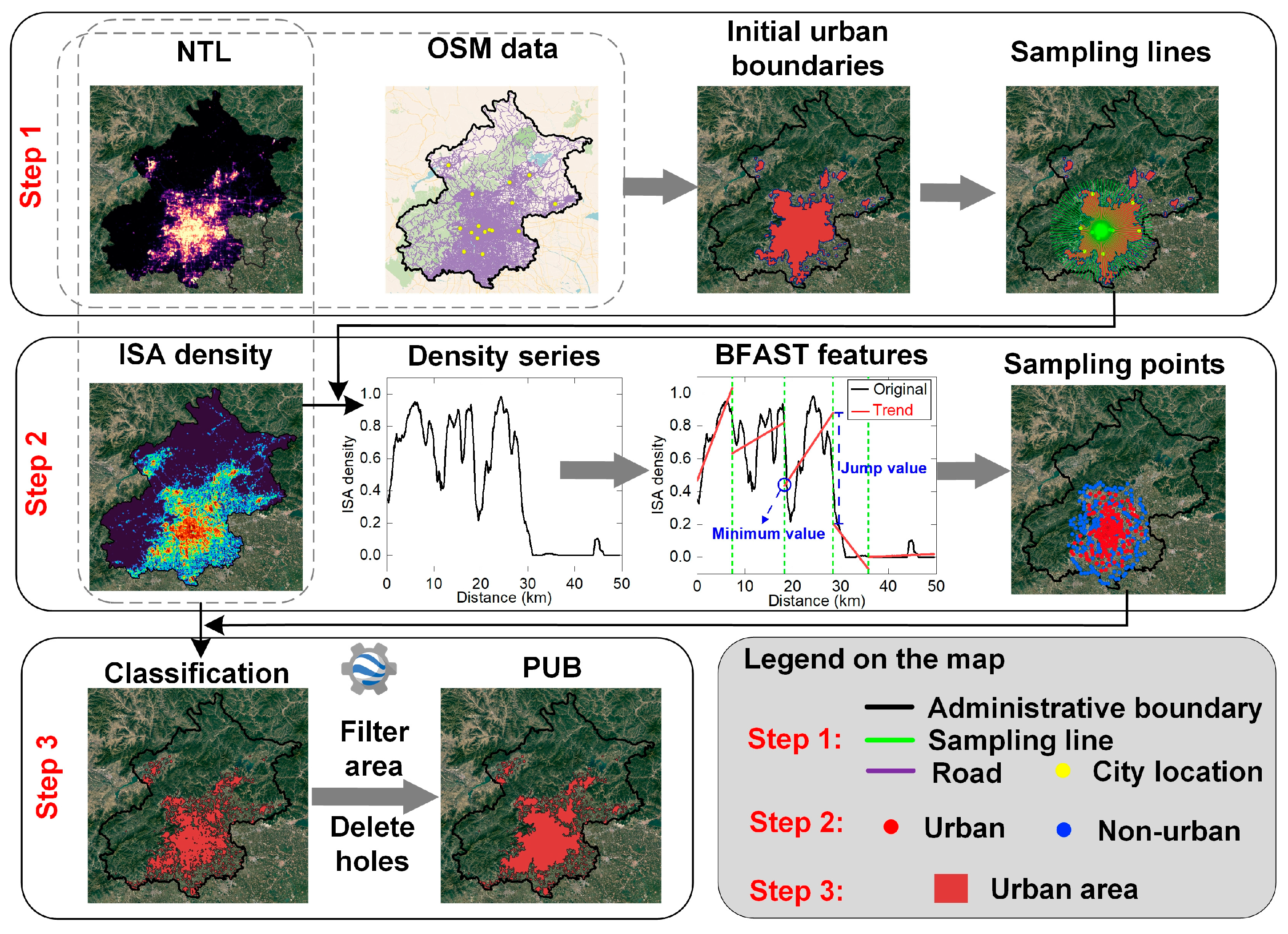
3.1. Initial Urban Boundary

Nighttime light data and road data are widely used in the extraction of urban built-up areas and the delineation of PUBs [35,36,37]. However, due to their limited spatial resolution, they can only be roughly used to preliminarily delineate the urban boundary. We briefly introduce the generation steps of the initial urban boundary:

(a)

Nighttime light maximum image synthesis. We assume that urban development is irreversible. Even if the urban development center may move, resulting in a decrease in the brightness of lights in some local areas, we still consider these local areas to have urban attributes. Therefore, an image with the maximum in every raster unit is synthesized by taking the maximum value of the nighttime light images over the years.

(b)

Nighttime light outlier handling. NPP/VIIRS data is sensitive to light brightness and is easily affected by bright scenes, such as fire areas and airport lights. Beijing is one of the most prosperous cities in China, and the maximum light value, except for the airport, is selected as the maximum value of urban light in the country. If the light value is greater than the set maximum value, the value will be assigned to the set maximum value.

(c)

Kernel density estimation for road nodes. Based on OpenStreetMap road nodes (Figure S1), kernel density estimation is performed. The kernel density radius is set to 1000 m [38], and 1/10 of the radius was used as the raster resolution for the calculation results [39] to obtain its kernel density map (Figure S2).

(d)

Initial urban boundary extraction. The nighttime light data and the kernel density map are normalized and subsequently multiplied. Then, the initial urban boundary (independent area > 2 km²) [40] is obtained based on the threshold method and morphological processing (Figure S3).

Obviously, in the process of generating the initial urban boundary, only preliminary urban boundaries can be obtained. The extraction results are affected by the blooming effect of the nighttime light data [41], the update and accuracy of the volunteered road data, the subjective awareness of the threshold method, etc. Therefore, the initial urban boundary may overestimate the developed cities and underestimate the developing cities, especially those cities with fewer crowdsourced data updates due to fewer volunteers (Figure S4).

3.2. Sampling Line

The sampling line is set up as a radial line extending outward from the city center. Therefore, the city center point and the radius of the radial lines need to be determined. For the city center point, the OpenStreetMap city place name and the initial urban boundary will be used to obtain the city center point. First, the largest independent patch of the initial urban boundary is selected in Beijing’s administrative boundary. Then, all the city place names in the independent patch will be obtained. If the number of points is greater than 1, the median coordinate of the point collection will be used as the city center point. For the radius of the radial line, the maximum distance from the city center point to the initial urban boundary will be used as the radius of the radial line. It is worth mentioning that the initial urban boundary can restrict the location of the sampling line to avoid the sampling line being influenced by subjective factors.

The size of the sampling line can be determined by the city center point and the radius obtained in the above way. Moreover, we set up an equal division of 90 sampling lines so as not to make the sampling lines too dense, resulting in sampling points that are not spatial-independent.

Scale plays a crucial role in cartography and spatial analysis. It determines the level of detail and accuracy in the representation of geographic features on a map. A larger scale means that features are represented more accurately, while a smaller scale may not accurately represent smaller features or distances. However, some PUB extraction approaches have the problem of scale inconsistency. Figure 2 illustrates the scale inconsistency problem caused by different sampling strategies.

Based on the natural principle theory [42], when mapping geographic elements, the more vertices, the more detailed the description of the features. In other words, the density of vertices per unit distance will describe the corresponding scale. In Figure 2a, parts 1–5 describe rough boundaries due to the long line segment, while parts 6–8 describe more detailed boundaries. Similarly, in Figure 2b, the more outward, the rougher the boundary description. The features of the real world are complex. Therefore, when these two strategies map boundaries, there will be problems with inconsistent cartographic scales even in the same boundary. In Figure 2c, by making the grid, the mutation points become denser compared to the previous strategies. However, this strategy actually dilutes the cartographic scale, which makes it difficult to truly express the shape of the actual land type in the boundary products. Even though mutation points are identified on each sampling line, scale inconsistencies still exist on some local boundaries.

Therefore, to avoid inconsistent scaling problems, we no longer directly connect mutation points. Instead, we further process these points as training samples for supervised machine learning classification.

3.3. Sampling Impervious Surface Density Series

Impervious surface is an important part of the urban landscape and a key feature reflecting urbanization. Figure S5 shows the impervious surface of Beijing in 2020. The impervious surface density can reflect the degree of urbanization within a specific range. Transitioning from the city center to suburban and then rural areas, the impervious surface density gradually decreases, and this indicative feature can be reflected in the density series. The impervious surface density is calculated as follows:

$$ISAD=\frac{P_{ISA}}{P_{all}}$$

(1)

where P_ISA denotes the number of impervious surface pixels in the area of a 33 × 33 pixel matrix, P_all denotes the number of all pixels in the area, and ISAD represents the impervious surface density of the central pixel of the area.

After obtaining the impermeable surface density image (Figure S6), the image will be sampled by the sampling line layer to obtain the density series, which will be subjected to mutation detection to obtain points with attributes.

3.4. Pretext Task in the Self-Supervised Learning Approach

The pretext task is used to obtain useful representations from unlabeled data by an objective function. For a binary classification task, the pretext task should automatically generate positive and negative samples provided to the downstream task for further learning. In this study, the pretext task automatically obtains training samples characterizing urban and non-urban areas by a mutation detection algorithm. However, we need an adaptive algorithm instead of the one with subjective parameters. Taking the SCWT algorithm, for example, different wavelet basis functions or even different sliding window sizes will give different mathematical meanings to the mutation points.

Therefore, we introduce an unsupervised mutation detection algorithm, BFAST. It is often used in additive time series [43,44], which can avoid subjective parameter setting to obtain objective results. In particular, BFAST usually decomposes the time series into trend item, seasonal item, and residual item based on the seasonal decomposition of the time series by Loess [45]. Then, the number of mutation points is determined by the Bayesian information criterion. After that, the ordinary least squares residual moving sum method is used to detect components where there is at least one significant breakpoint. Finally, the component is fitted piecewise linearly by significance calculation (p < 0.05) to determine the breakpoint locations. The decomposition component and piecewise linear fit are iterated until convergence.

For these imperious surface density series, the impervious surface density map has strong spatial heterogeneity, resulting in no periodicity in the series. Therefore, the sampling series of impervious surface density is considered an additive series of trend items and residual items. Then, the series detects mutation points by the BFAST algorithm, obtaining the urban-to-non-urban mutation points. However, these points cannot clearly represent urban or non-urban attributes, and it is necessary to distinguish binary attributes based on the features detected by BFAST. Figure S7 shows the impervious surface density series sampled by a sampling line in Beijing and its features after BFAST detection. To this end, we take these sub-series segmented by mutation points to determine the binary attributes of these points based on their BFAST features. These points will be used as training samples and validation samples for the downstream task.

3.5. Downstream Task in the Self-Supervised Learning Approach

In the downstream task, the supervised information obtained in the pretext task can be put into supervised learning to perform classification, segmentation, prediction, etc. In this study, our downstream task is a binary classification task with positive and negative samples obtained in the pretext task, which enables supervised learning to further characterize urban and non-urban areas.

The SVM is chosen as the classifier in GEE. Samples, nighttime light maximum images, and impervious surface density data will be fed into the classifier to extract PUBs. Specifically, first, sampling points with attributes will be divided into 70% training data and 30% validation data. Then, the sampled features are impervious surface density and nighttime light maximum, and these data will be classified by the SVM classifier. Finally, we filter some non-urban patches (patch-independent area < 2 km²) [40]. Moreover, we fill the voids within the urban area, which are the green spaces and water bodies, carrying urban functions.

After these post-processing steps, we map CPUBs in 1995, 2000, 2005, 2010, 2015, and 2020. Noteworthily, due to the unsaturation of DMSP data and the non-uniform values of the two nighttime light data, we use the overlap part of the two types of nighttime light data in 2012 and 2013 to perform linear regression and convert the DMSP to VIIRS-like images. Moreover, the sampling points are obtained based on impervious surface density data calculated separately for each temporal. Therefore, even if there are deviations between different nighttime light values in multi-temporal data, for independent training data, they do not interfere with the classification results.

4. Results

4.1. Characteristics of CPUB

Figure 3 shows the spatial extent of CPUB urban areas in the Beijing–Tianjin region and Hefei City, Anhui Province, in 2020. CPUB is overlaid on the high-resolution Google Earth image basemap, and it can be clearly observed that CPUB matches well with the spatial extent of the actual urban areas, indicating that CPUB can distinguish urban areas and non-urban areas well.

The Beijing–Tianjin region demonstrates the urban-scale PUB. For the six local enlarged maps, CPUB can accurately capture the PUB, and can still accurately identify places on the urban edge far from the city center (Figure 3a). The actual development and construction of the city, connecting to the overall urban spatial extent, can be identified instead of being identified as non-urban. Hefei shows the more detailed spatial extent of the urban areas. Based on the Hefei high-resolution image basemap, our results can map the PUBs well. In the local details of the six building-scale urban edges, patches of buildings are accurately mapped to their boundaries, indicating that CPUB can accurately quantify the urban boundaries.

By overlaying CPUB on high-resolution satellite images, CPUB matches well with the spatial extent of the actual urban area. Therefore, CPUB is a reliable and accurate product and can describe the actual urban areas at the urban scale and building scale.

To observe the dynamic changes of multi-temporal CPUBs, we show PUBs and the initial urban boundaries of Chengdu in Sichuan Province, Hefei in Anhui Province, Wuhan in Hubei Province, and Xi’an in Shaanxi Province in Figure 4. From 1995 to 2020, CPUB can describe the dynamic changes of PUBs, and all four cities have experienced obvious growth. We superimpose the urban boundaries on satellite images, and it can be clearly observed that our results describe the urban area extent well. For the initial urban boundary, in general, the urban form is consistent with CPUB. However, the initial urban boundary is overestimated compared to CPUB because the threshold method is difficult to accurately segment urban and non-urban. The light brightness at the edges of prosperous cities is significantly stronger than at the edges of less developed areas, which is one of the reasons why the initial urban boundary is underestimated in Figure S4.

4.2. Comparison with Other Products

In order to evaluate CPUB accurately, it will be compared with global urban boundaries (GUBs). The GUB is a physical urban boundary dataset produced by secondary processing of impervious surface data based on kernel density estimation and cellular automata methods [22]. The latest temporal of the GUB dataset has been updated to 2020. In order to verify the effectiveness of CPUB, we performed a visual comparison and quantitative accuracy verification of these two products.

Figure 5 shows the PUBs of Hefei and Xi’an. For the overall of the two cities, the GUB in 2020 is larger than CPUB in 2020, indicating that the GUB may slightly overestimate the boundaries. To this end, we randomly selected six parts at the edges of the two cities to display their details. In the six local enlarged maps of Hefei, the area included in the GUB but not in CPUB contains some agricultural land and few buildings. These six areas are far away from the main body of the city and should be defined as rural areas. Therefore, CPUB can accurately distinguish between urban and non-urban areas. Similarly, in the six local enlarged maps of Xi’an, except for Xi’an(g) (Figure 5g), other submaps are dominated by agricultural land. For Xi’an(g) (Figure 5g), the area is a cluster of villages and contains a large amount of cropland, so it is considered rural.

In addition to the visual comparison, we also compare the two datasets by a quantitative accuracy evaluation. We select ten different cities with different locations, sizes, and development levels. These cities are Shanghai, Chengdu, Xi’an, Wuhan, Hefei, Changsha in Hunan Province, Linyi in Shandong Province, Xuzhou in Jiangsu Province, Yancheng in Jiangsu Province, and Weifang in Shandong Province. Then, 200 points are randomly generated for each city. Below, we describe, in detail, the process of generating these samples. The central areas of cities are difficult to classify as non-urban areas. Thus, we do not set sample points at the central areas of the cities. On the contrary, the edge areas of the cities are more likely to be misidentified (Figure 5). Therefore, our accuracy verification experiments should be designed to pay more attention to the urban fringe. Firstly, we buffer the selected urban boundaries, and the radius of the buffer is 2.5 km. Then, we randomly generate 200 points in the buffer polygon, and these points cannot be less than 300 m away from each other to ensure their spatial independence. Finally, each point is visually interpreted by two urban research experts based on high-resolution Google Earth images.

We counted the confusion matrix and calculated producer accuracy (PA), user accuracy (UA), overall accuracy (OA), and F1-score in

Table 1. Confusion matrix of CPUB and GUB products in 2020 and their accuracy assessments.

CPUB	Urban	Non-Urban	UA	GUB	Urban	Non-Urban	UA
Urban	837	45	94.9%	Urban	885	535	62.3%
Non-urban	69	1049		Non-urban	21	559
PA	92.4%			PA	97.7%
OA	94.3%	F1-score	93.6%	OA	72.2%	F1-score	76.1%

. We take the PUB extraction as an example to explain the meaning of these indicators. PA is the ratio of urban attribute samples that are correctly classified to real urban samples. UA is the ratio of urban attribute samples that are correctly classified to those that are judged to be urban attributes by the boundary dataset. OA represents the ratio of all correctly classified samples to all samples. The F1-score conveys the balance between PA and UA.

Firstly, both datasets have relatively high PAs, indicating that both datasets enclose the city well. The UA of CPUB reaches 94.9%, indicating that CPUB excludes non-urban areas. However, the UA of the GUB is only 62.3%, which shows that the GUB overestimates the urban extent and includes many non-urban areas. For both the OA and F1-score, the values of CPUB are above 90%, indicating that CPUB can extract physical urban boundaries well. However, the values of the GUB are significantly lower than CPUB, which shows that the GUB does not distinguish between urban and non-urban areas. This is consistent with the evaluation of the GUB given in the literature [9]. The reason why the GUB overestimates the urban extent may be because the impervious surface also exists in rural areas, and the impervious surface in rural areas is mistakenly classified as urban land.

In general, CPUB has a finer-grained ability to delineate the boundaries than existing products and can effectively distinguish urban and non-urban areas. Therefore, it can be considered that CPUB is a highly credible PUB product.

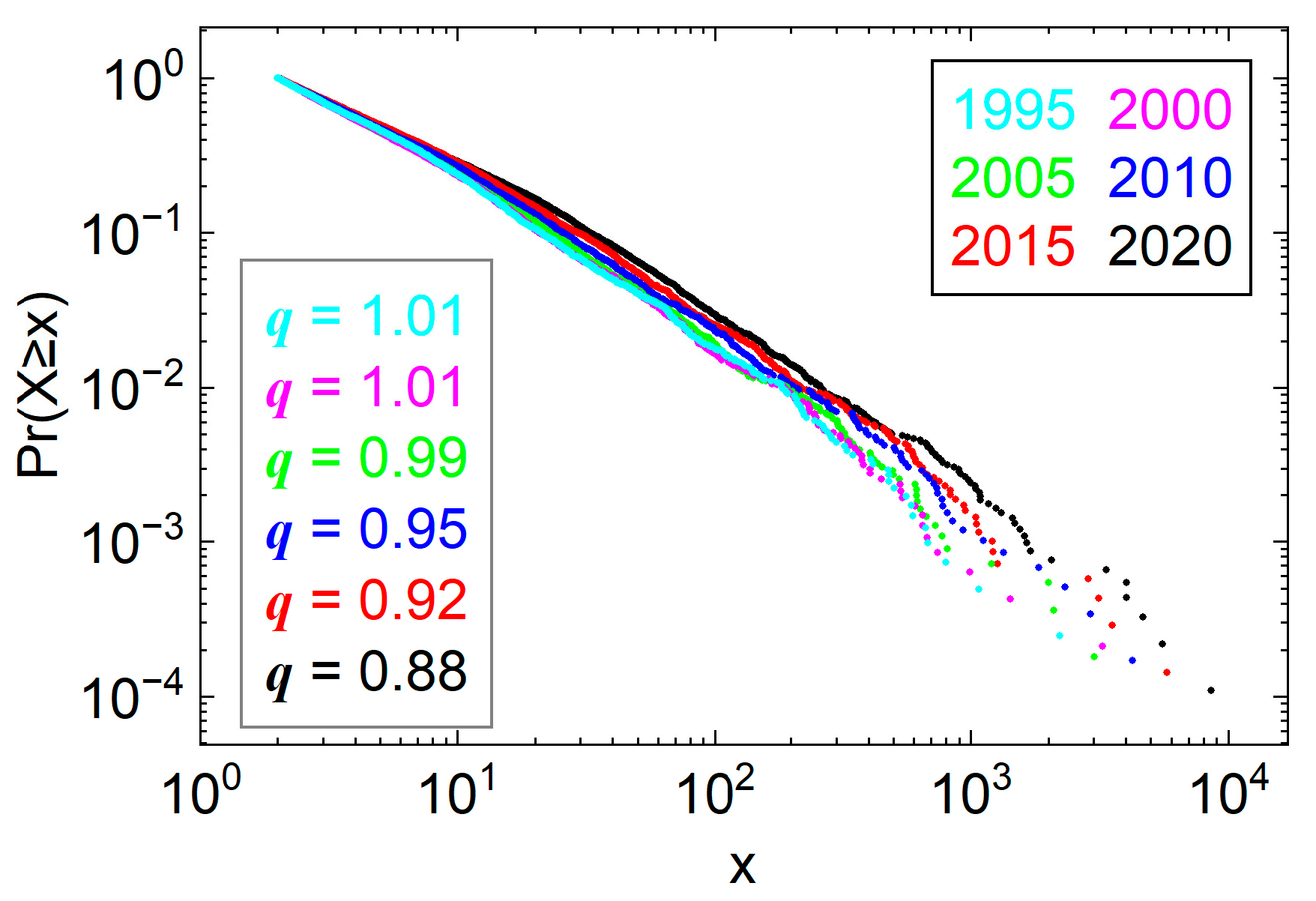
4.3. Size Rank Characteristics of Chinese Cities

We rank the cities for analyzing urban development from 1995 to 2020 (Figure 6). In 1995, the number of cities in China is 4077; by 2020, the number of cities has increased to 9164, which is 2.2 times that of 1995. For the large cities (an area greater than 100 km²), there are 72 in 1995; by 2020, the number of large cities has increased to 269, which is 3.7 times that of 1995. Moreover, with the acceleration of China’s urbanization process, the difference in China’s urban areas is increasing, and the number of non-large cities is increasing, which shows that Chinese cities are actively developing overall. Furthermore, the city rank of the GUB statistics (Figure S8) is basically consistent with our results.

Zipf’s law is one of the most significant empirical facts in the ranking of city size [46,47]. It is generally believed that the city’s size is inversely proportional to its rank of size. We give the mathematical expression of Zipf’s in the rank size as follows:

$$S_i=S_1\ast R_i{}^{-q}$$

(2)

where S_i denotes the size of the i-th city, S₁ denotes the size of the largest city, R_i denotes the rank of the i-th city, and q denotes Zipf’s exponent. Obviously, city size is inversely proportional to the rank of the city. Moreover, when the city size obeys a power law distribution and q is close to 1, it can be considered to be in line with Zipf’s law [19]. To characterize the power law distribution of city size, formula (2) can be equivalent to:

$$\mathrm{Pr}\left(X\ge x\right)=r^{-q}$$

(3)

where $\mathrm{Pr}\left(X\ge x\right)$ represents the probability that the number of cities with a size greater than x in all cities accounts for the number of all cities and r represents the rank of the probability of the number of cities with a size greater than x among all cities in the probability set. For example, if there are 10 cities and the set of city sizes is from 1 to 10, the probability of the cities with sizes larger than the smallest city, $\mathrm{Pr}\left(X\ge x\right)$ is equal to 1.

Figure 7 shows Zipf’s distribution of Chinese cities from 1995 to 2020. We define the cut-off size of the city in advance, so the beginnings of Zipf’s distributions of these six groups of Chinese cities are coincident. We fit the area size of Chinese cities, and Zipf’s exponents are shown in Figure 7. Zipf’s exponents are close to 1; however, with the continuous development of Chinese cities, Zipf’s exponent has decreased from 1.01 in 1995 to 0.88 in 2020. In terms of the exponent in China, the development status of Chinese cities has changed from the coordinated development of large, medium, and small cities to insufficient development of small and medium cities. Furthermore, Zipf’s distribution of our results is basically consistent with the GUB statistics (Figure S9).

5. Discussion

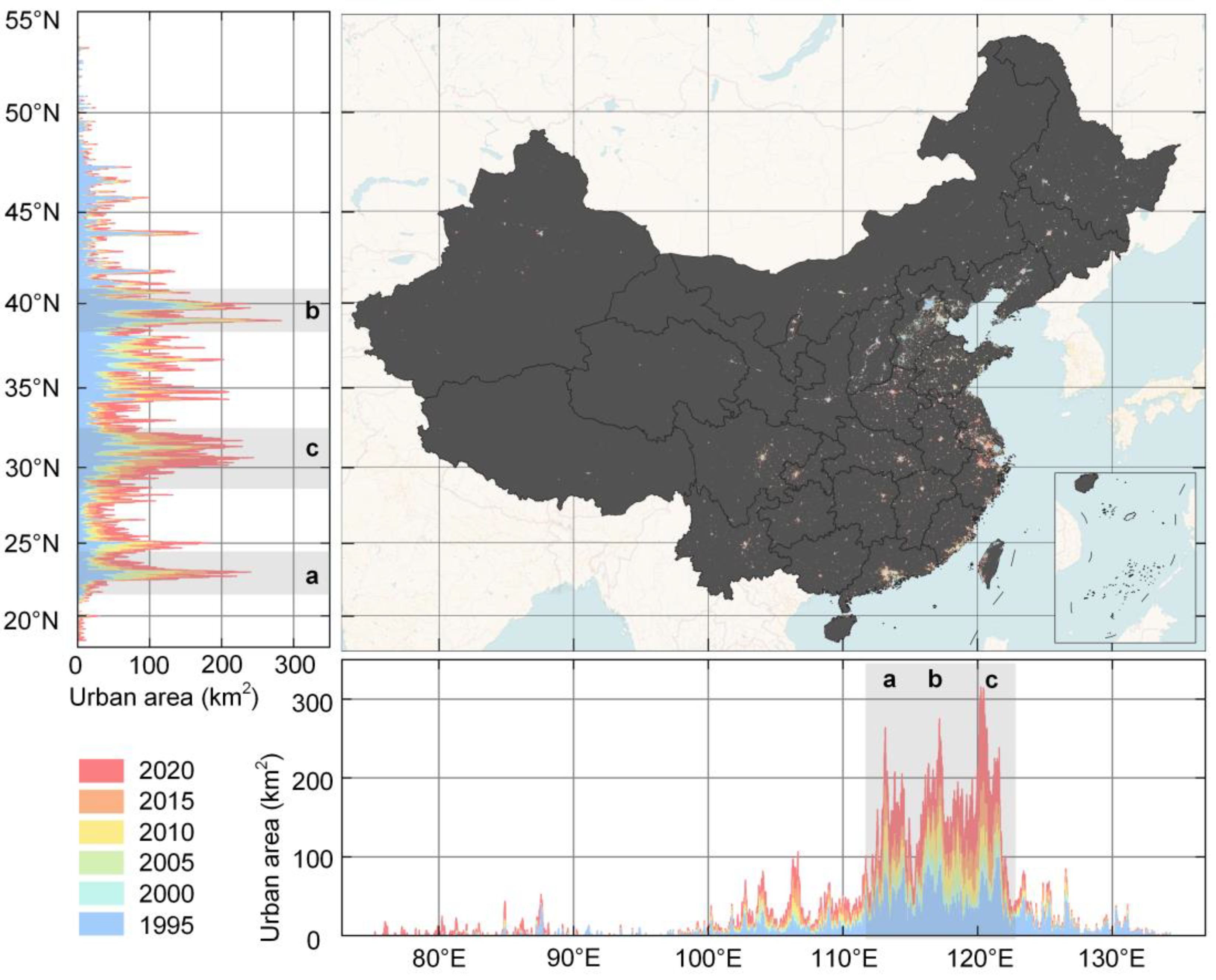
5.1. Regional SpatioTemporal Dynamics of Chinese Cities

In order to explore the regional development of Chinese cities, we use the provinces where the nine major urban agglomerations in China are located as the spatial extent to conduct regional spatiotemporal dynamic analysis. The province collection of these urban agglomerations and their locations are presented in Table S1 and Figure S10. The nine urban agglomerations are the Beijing–Tianjin–Hebei region (BTH), Yangtze River Delta (YRD), Guangdong–Hong Kong–Macao Greater Bay Area (GBA), the Three Northeastern Provinces (TNPs), Shandong Peninsula Urban Agglomeration (SPUA), Triangle of Central China (TCC), Chengdu–Chongqing City Group (CCCG), Guanzhong Plain City Group (GPCG), Central Plains Urban Agglomeration (CPUA).

We counted the overall urban area of China in the longitude and latitude directions (Figure 8). For the statistical results in the longitude direction, there are three obvious area peaks in the mask, marked a, b, and c, which correspond to GBA, BTH, and YRD, respectively. Moreover, in areas greater than 110°E, the urban area accounts for 89.3% of China’s total urban area in 1995, and this ratio is 86.3% in 2020. For the statistical results in the latitude direction, the three regions also have high peaks, and the peak around 35°N points to CPUA. Similarly, in areas less than 40°N, the urban area accounts for 74.2% of China’s total urban area in 1995, and this ratio is 83.5% in 2020. In general, China’s urban development center has moved westward and southward. China’s urban development has a phenomenon of uncoordinated regional development at the national scale.

At the regional scale, the spatiotemporal dynamics of urban development intensification are also worthy of attention in regional urban development. Therefore, we analyze the urban development intensification in the areas where the nine urban agglomerations are located (Figure 9).

It can be seen in Figure 9 that the urban areas of all regions are growing, among which YRD, TCC, and CPUA have seen rapid urban area growth since 2010, while the TNPs have grown slowly. For the ratio of impervious surface and urban area (urban land intensification), both GBA and GPCG are at a high level of intensification, which may be due to the fact that the plains of Guangdong Province only account for 21.7% of the province’s land area [48], resulting in the forced intensive development of the cities. Likewise, GPCG has a small amount of plain area, which may be one of the reasons contributing to the intensification. Moreover, in 1995 and 2000, urban space has strong aggregation and intensification. With the development of cities, urban sprawl generally occurs in cities with high-speed construction, and some urban agglomerations ignore the intensive construction of cities, such as TCC, CCCG, and CPUA.

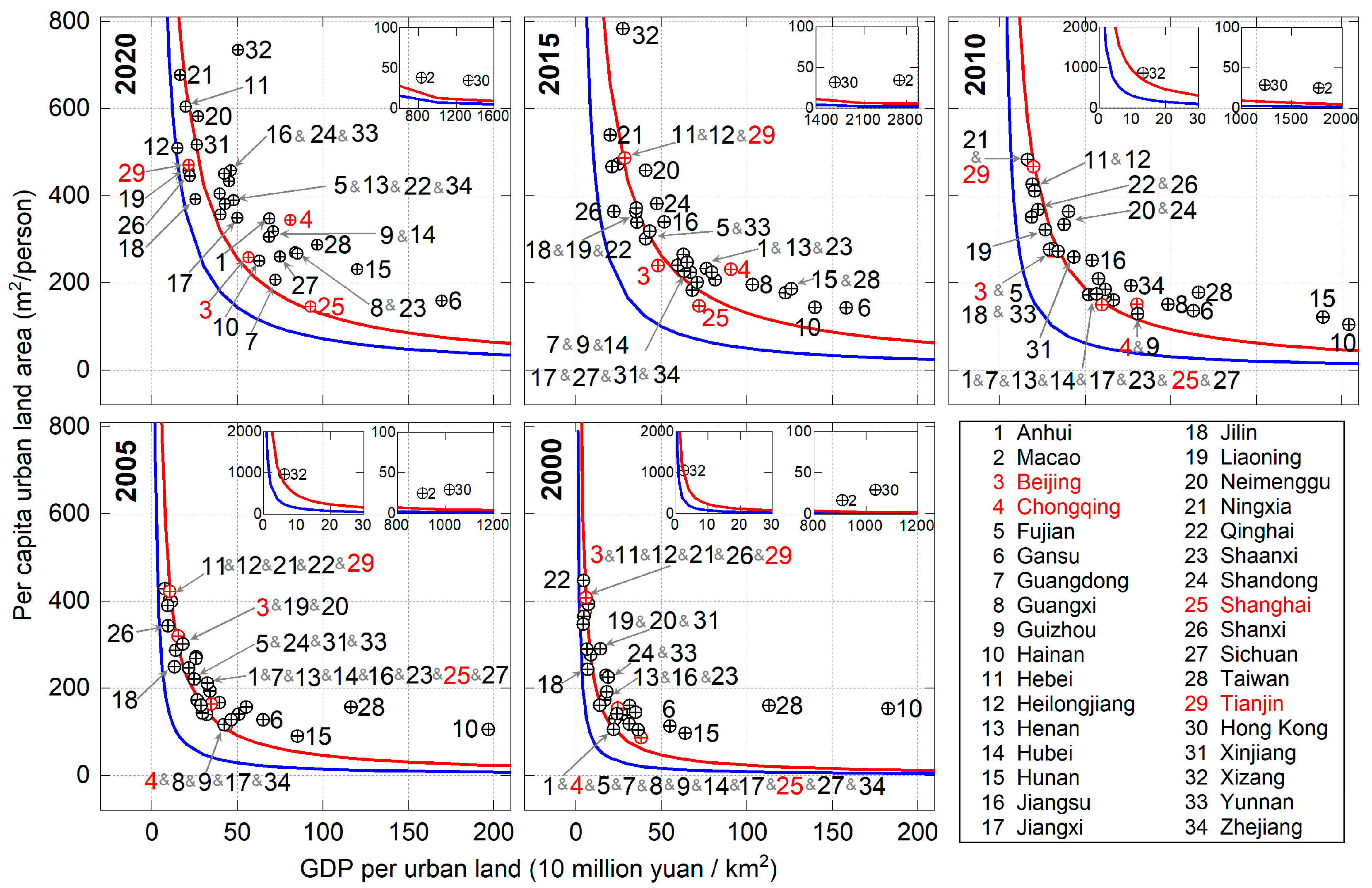
5.2. Urbanization in Chinese Provinces

Urbanization assessment requires not only the calculation of the urban area but also the analysis of the urban economy and urban population. Therefore, we collected GDP data from the China City Statistical Yearbook and the 100 m resolution population raster data from WorldPop [49] in 2000, 2005, 2010, 2015, and 2020 for assessing urban development in China’s provinces and cities. The GDP data of Hong Kong, Macao, and Taiwan comes from the International Monetary Fund [50]. Noteworthily, when counting urban GDP, only the sum of the secondary industry and the tertiary industry is counted; that is, the GDP is produced by non-agricultural activities because the economic development of the city is mainly supported by the secondary industry and tertiary industry.

The development of a city is inseparable from the GDP volume of the city, and GDP growth requires the expansion of the city’s size to increase the city’s development potential. Hence, we calculated the relationship between the urban area and GDP in each province (Figure 10). We consider the area of a city to be positively correlated with GDP and assume that the two obey a linear relationship; that is, y = k × x, where x means the urban area, y means the GDP, and k means the slope of the fitted line. In Figure 10, the linear relationship can fit the distribution of the two well with a good fitting effect, except for 2000. In addition, the fitted slope from 2000 to 2015 shows an upward trend, indicating that urban expansion brings more GDP. In 2015, the conversion ratio of the urban area to GDP reaches its peak (4.8). However, from 2015 to 2020, the economic conversion ratio generated by urban expansion has slightly decreased, but it still has a good performance. In general, cities need to be developed more intensively to maximize the economic conversion ratio. Similarly, we show the relationship between the urban area and GDP at the city level (Figure S11), and the results are basically consistent with those at the province level.

To meticulously analyze the urban intensification in each province, we correlate the urban area with the corresponding economic and population data and calculate indicators reflecting the urban intensification [51]. The GDP per urban land (I_gp) and the per capita urban land (I_ap) are calculated as follows:

$$I_{gp}=\frac{\mathrm{GDP}\ast \left(1-f\right)}{S_a}$$

(4)

$$I_{ap}=\frac{S_a}{P_{op}}$$

(5)

where f represents the ratio of the primary industry in the GDP, S_a represents the area of the city, and P_op represents the population counts within the spatial extent of the corresponding PUB. Obviously, the per urban capita GDP is obtained by multiplying the above two formulas together. When taking I_gp and I_ap as the x and y axes, respectively, the per urban capita GDP at this time is expressed as an inversely proportional function, which is a contour line (y = a/x, a is the urban per capita GDP) in the first quadrant.

Figure 11 shows the distribution of urban intensification indicators in each province of China. From 2000 to 2020, most of the provinces show an increasing trend in the GDP per urban land and the per capita urban land, indicating that the aggregation of urban population and urban economic potential are both well-represented. We have marked in red four Chinese municipalities: Beijing (3), Chongqing (4), Shanghai (25), and Tianjin (29).

In 2000, Beijing and Tianjin have a high level of per capita urban land and a low level of GDP per urban land, while Chongqing and Shanghai develop more reasonably at the same time. By 2020, the two indicators of Tianjin are still similar to those in 2000. This may be attributed to the fact that Tianjin is a port and transportation city that requires significant land for construction to fulfill its urban functions. Shanghai in 2020 has a high level of urban intensification and a high economic output of urban land because the dense population leads to these phenomena. Heilongjiang (12), Jilin (18), and Liaoning (19) in the TNPs were always in a low-intensive urban state, which may be the reason for the insufficient utilization of urban space due to population loss in these areas [52,53].

The two contour lines (Figure 11) represent the national per capita GDP (blue) and the province-level average per urban capita GDP (red).

Table 2. Statistical results of the national per capita GDP and the province-level average per urban capita GDP.

Year	2000	2005	2010	2015	2020
National per capita GDP (CNY)	7900	14,400	30,800	49,900	71,800
Province-level average per Urban capita GDP (CNY)	23,300	45,700	92,900	131,100	128,000
Ratio	2.9	3.2	3.0	2.6	1.8

gives their values and ratios. The results show that the national per capita GDP and the province-level average per urban capita GDP are basically increasing. The ratios of these two indicators reaches a peak in 2005, and then begins to decrease, which shows that the overall gap between rich and poor in China began to gradually decrease.

Urban expansion drives GDP growth, which accelerates China’s urbanization process. The conversion ratio between the urban area and the urban economy is significant, and the intensification of Chinese cities is increasing. In Figure S12, the urban intensification has a regional and clustered distribution, which reveals that China’s urbanization requires regional coordinated development. Moreover, the ratios between the city-level average per urban capita GDP and the national per capita GDP also show that the gap between rich and poor in China is gradually decreasing.

6. Conclusions

In this study, we developed a self-supervised learning approach for extracting physical urban boundaries that was driven by multi-source data without any subjective parameter constraints and priori labeled samples, generating CPUB dataset including in 1995, 2000, 2005, 2010, 2015, and 2020. Firstly, we set a sampling line layer to obtain the series of impervious surface density data. Then, based on the unsupervised mutation detection algorithm, BFAST, designed as a pretext task, the samples representing urban and non-urban attributes were automatically generated. Finally, a supervised learning task, the SVM in GEE, was designed as a downstream task to classify the PUB. In this way, the problem of scale inconsistency caused by only connecting mutation points to delineate urban boundaries can be avoided. When extracting PUBs, automatic rather than manual boundary mapping can be realized.

CPUB can accurately describe the spatial extent of the urban area at both the city scale and the building scale. It is capable of effectively capturing the expansion of cities. Compared with the GUB, CPUB can better distinguish rural and urban areas. The size rank characteristics of Chinese cities follow Zipf’s law, which has good agreement with the existing dataset. Furthermore, our analysis of the regional spatiotemporal dynamics of Chinese cities reveals that the development center of Chinese cities has shifted westward and southward. By calculating the relationship between urban area, population, and economy, we also find that the conversion ratio of urban area to GDP is increasing, with a peak in 2015 and a subsequent slight decrease. Meanwhile, the intensification of Chinese cities is increasing, and the gap between rich and poor in China is decreasing.

In general, the proposed method combines the advantages of mutation detection and a data-driven strategy to provide a new baseline method for urban boundary extraction research. CPUB can provide high-confidence base data for urban monitoring, urban management, and spatial planning. In future work, we will continuously update this dataset to provide immediate and effective geographic information services for urban research.

References

1. Guan, X.; Wei, H.; Lu, S.; Dai, Q.; Su, H. Assessment on the urbanization strategy in China: Achievements, challenges and reflections. Habitat Int. 2018, 71, 97–109. [Google Scholar] [CrossRef]
2. Chen, M.; Zhang, H.; Liu, W.; Zhang, W. The global pattern of urbanization and economic growth: Evidence from the last three decades. PLoS ONE 2014, 9, e103799. [Google Scholar] [CrossRef] [Green Version]
3. Song, X.P.; Hansen, M.C.; Stehman, S.V.; Potapov, P.V.; Tyukavina, A.; Vermote, E.F.; Townshend, J.R. Global land change from 1982 to 2016. Nature 2018, 560, 639–643. [Google Scholar] [CrossRef] [PubMed]
4. Li, Y.; Li, X.; Lu, T. Coupled Coordination Analysis between Urbanization and Eco-Environment in Ecologically Fragile Areas: A Case Study of Northwestern Sichuan, Southwest China. Remote Sens. 2023, 15, 1661. [Google Scholar] [CrossRef]
5. Cumming, G.S.; Buerkert, A.; Hoffmann, E.M.; Schlecht, E.; von Cramon-Taubadel, S.; Tscharntke, T. Implications of agricultural transitions and urbanization for ecosystem services. Nature 2014, 515, 50–57. [Google Scholar] [CrossRef] [PubMed]
6. Liu, X.; Huang, Y.; Xu, X.; Li, X.; Li, X.; Ciais, P.; Lin, P.; Gong, K.; Ziegler, A.D.; Chen, A.; et al. High-spatiotemporal-resolution mapping of global urban change from 1985 to 2015. Nat. Sustain. 2020, 3, 564–570. [Google Scholar] [CrossRef]
7. Seto, K.C.; Fragkias, M.; Guneralp, B.; Reilly, M.K. A meta-analysis of global urban land expansion. PLoS ONE 2011, 6, e23777. [Google Scholar] [CrossRef]
8. Zhou, Y.; Shi, Y. Toward establishing the concept of physical urban area in China. Acta Geogr. Sin. 1995, 50, 289–301. (In Chinese) [Google Scholar]
9. Zhang, X.; Du, S.; Zhou, Y.; Xu, Y. Extracting physical urban areas of 81 major Chinese cities from high-resolution land uses. Cities 2022, 131, 104061. [Google Scholar] [CrossRef]
10. Zhen, F.; Cao, Y.; Qin, X.; Wang, B. Delineation of an urban agglomeration boundary based on Sina Weibo microblog ‘check-in’ data: A case study of the Yangtze River Delta. Cities 2017, 60, 180–191. [Google Scholar] [CrossRef]
11. Yin, J.; Soliman, A.; Yin, D.; Wang, S. Depicting urban boundaries from a mobility network of spatial interactions: A case study of Great Britain with geo-located Twitter data. Int. J. Geogr. Inf. Sci. 2017, 31, 1293–1313. [Google Scholar] [CrossRef] [Green Version]
12. Li, Y.; Sun, Q.; Ji, X.; Xu, L.; Lu, C.; Zhao, Y. Defining the Boundaries of Urban Built-up Area Based on Taxi Trajectories: A Case Study of Beijing. J. Geovis. Spat. Anal. 2020, 4, 1–12. [Google Scholar] [CrossRef]
13. Tannier, C.; Thomas, I. Defining and characterizing urban boundaries: A fractal analysis of theoretical cities and Belgian cities. Comput. Environ. Urban Syst. 2013, 41, 234–248. [Google Scholar] [CrossRef]
14. Tannier, C.; Thomas, I.; Vuidel, G.; Frankhauser, P. A Fractal Approach to Identifying Urban Boundaries. Geogr. Anal. 2011, 43, 211–227. [Google Scholar] [CrossRef]
15. Li, X.; Zheng, K.; Qin, F.; Wang, H.; Zhao, C. Deriving Urban Boundaries of Henan Province, China, Based on Sentinel-2 and Deep Learning Methods. Remote Sens. 2022, 14, 3752. [Google Scholar] [CrossRef]
16. Dai, X.; Jin, J.; Chen, Q.; Fang, X. On Physical Urban Boundaries, Urban Sprawl, and Compactness Measurement: A Case Study of the Wen-Tai Region, China. Land 2022, 11, 1637. [Google Scholar] [CrossRef]
17. Hu, S.; Tong, L.; Frazier, A.E.; Liu, Y. Urban boundary extraction and sprawl analysis using Landsat images: A case study in Wuhan, China. Habitat Int. 2015, 47, 183–195. [Google Scholar] [CrossRef]
18. Rozenfeld, H.D.; Rybski, D.; Andrade Jr, J.S.; Batty, M.; Stanley, H.E.; Makse, H.A. Laws of population growth. Proc. Natl. Acad. Sci. USA 2008, 105, 18702–18707. [Google Scholar] [CrossRef] [Green Version]
19. Jiang, B.; Jia, T. Zipf’s law for all the natural cities in the United States: A geospatial perspective. Int. J. Geogr. Inf. Sci. 2011, 25, 1269–1281. [Google Scholar] [CrossRef]
20. Oliveira, E.A.; Furtado, V.; Andrade, J.S.; Makse, H.A. A worldwide model for boundaries of urban settlements. Roy. Soc. Open Sci. 2018, 5, 180468. [Google Scholar] [CrossRef] [Green Version]
21. Liu, S.; Shi, K.; Wu, Y. Identifying and evaluating suburbs in China from 2012 to 2020 based on SNPP–VIIRS nighttime light remotely sensed data. Int. J. Appl. Earth Obs. Geoinf. 2022, 114, 103041. [Google Scholar] [CrossRef]
22. Li, X.; Gong, P.; Zhou, Y.; Wang, J.; Bai, Y.; Chen, B.; Hu, T.; Xiao, Y.; Xu, B.; Yang, J.; et al. Mapping global urban boundaries from the global artificial impervious area (GAIA) data. Environ. Res. Lett. 2020, 15, 094044. [Google Scholar] [CrossRef]
23. Peng, J.; Hu, Y.n.; Liu, Y.; Ma, J.; Zhao, S. A new approach for urban-rural fringe identification: Integrating impervious surface area and spatial continuous wavelet transform. Landsc. Urban Plan. 2018, 175, 72–79. [Google Scholar] [CrossRef]
24. Yang, J.; Dong, J.; Sun, Y.; Zhu, J.; Huang, Y.; Yang, S. A constraint-based approach for identifying the urban–rural fringe of polycentric cities using multi-sourced data. Int. J. Geogr. Inf. Sci. 2022, 36, 114–136. [Google Scholar] [CrossRef]
25. Taubenböck, H.; Weigand, M.; Esch, T.; Staab, J.; Wurm, M.; Mast, J.; Dech, S. A new ranking of the world’s largest cities—Do administrative units obscure morphological realities? Remote Sens. Environ. 2019, 232, 111353. [Google Scholar] [CrossRef]
26. Schiappa, M.C.; Rawat, Y.S.; Shah, M. Self-supervised learning for videos: A survey. ACM Comput. Surv. 2022. [Google Scholar] [CrossRef]
27. Li, H.; Li, Y.; Zhang, G.; Liu, R.; Huang, H.; Zhu, Q.; Tao, C. Global and local contrastive self-supervised learning for semantic segmentation of HR remote sensing images. IEEE Trans. Geosci. Remote Sens. 2022, 60, 1–14. [Google Scholar] [CrossRef]
28. Zbontar, J.; Jing, L.; Misra, I.; LeCun, Y.; Deny, S. Barlow twins: Self-supervised learning via redundancy reduction. In Proceedings of the International Conference on Machine Learning, PMLR, Virtual, 18–24 July 2021; pp. 12310–12320. [Google Scholar]
29. Zhao, Z.; Luo, Z.; Li, J.; Chen, C.; Piao, Y. When Self-Supervised Learning Meets Scene Classification: Remote Sensing Scene Classification Based on a Multitask Learning Framework. Remote Sens. 2020, 12, 3276. [Google Scholar] [CrossRef]
30. Stojnic, V.; Risojevic, V. Self-supervised learning of remote sensing scene representations using contrastive multiview coding. In Proceedings of the IEEE/CVF Conference on Computer Vision and Pattern Recognition (CVPR), Nashville, TN, USA, 19–25 June 2021; pp. 1182–1191. [Google Scholar]
31. Heidler, K.; Mou, L.; Hu, D.; Jin, P.; Li, G.; Gan, C.; Wen, J.-R.; Zhu, X.X. Self-supervised audiovisual representation learning for remote sensing data. Int. J. Appl. Earth Obs. Geoinf. 2023, 116, 103130. [Google Scholar] [CrossRef]
32. Haklay, M.; Weber, P. Openstreetmap: User-generated street maps. IEEE Pervas. Comput. 2008, 7, 12–18. [Google Scholar] [CrossRef] [Green Version]
33. National Geomatics Center of China. 1: 1 Million Public Version of Basic Geographic Information Data. Available online: https://www.webmap.cn/commres.do?method=result100W (accessed on 29 March 2022).
34. Gorelick, N.; Hancher, M.; Dixon, M.; Ilyushchenko, S.; Thau, D.; Moore, R. Google Earth Engine: Planetary-scale geospatial analysis for everyone. Remote Sens. Environ. 2017, 202, 18–27. [Google Scholar] [CrossRef]
35. Liu, X.; Ning, X.; Wang, H.; Wang, C.; Zhang, H.; Meng, J. A Rapid and Automated Urban Boundary Extraction Method Based on Nighttime Light Data in China. Remote Sens. 2019, 11, 1126. [Google Scholar] [CrossRef] [Green Version]
36. Cheng, F.; Liu, S.; Hou, X.; Zhang, Y.; Dong, S.; Coxixo, A.; Liu, G. Urban land extraction using DMSP/OLS nighttime light data and OpenStreetMap datasets for cities in China at different development levels. IEEE J. Sel. Top. Appl. Earth Obs. Remote Sens. 2018, 11, 2587–2599. [Google Scholar] [CrossRef]
37. Zhou, Y.; Li, X.; Asrar, G.R.; Smith, S.J.; Imhoff, M. A global record of annual urban dynamics (1992–2013) from nighttime lights. Remote Sens. Environ. 2018, 219, 206–220. [Google Scholar] [CrossRef]
38. Wu, H.; Wang, L.; Zhang, Z.; Gao, J. Analysis and optimization of 15-minute community life circle based on supply and demand matching: A case study of Shanghai. PLoS ONE 2021, 16, e0256904. [Google Scholar] [CrossRef] [PubMed]
39. Li, F.; Yan, Q.; Bian, Z.; Liu, B.; Wu, Z. A POI and LST adjusted NTL urban index for urban built-up area extraction. Sensors 2020, 20, 2918. [Google Scholar] [CrossRef]
40. Jiang, Z.; Zhai, W.; Meng, X.; Long, Y. Identifying Shrinking Cities with NPP-VIIRS Nightlight Data in China. J. Urban Plan. Dev. 2020, 146, 04020034. [Google Scholar] [CrossRef]
41. Cao, X.; Hu, Y.; Zhu, X.; Shi, F.; Zhuo, L.; Chen, J. A simple self-adjusting model for correcting the blooming effects in DMSP-OLS nighttime light images. Remote Sens. Environ. 2019, 224, 401–411. [Google Scholar] [CrossRef]
42. Li, Z.; Openshaw, S. Algorithms for automated line generalization1 based on a natural principle of objective generalization. Int. J. Geogr. Inf. Sci. 1992, 6, 373–389. [Google Scholar] [CrossRef]
43. Masiliūnas, D.; Tsendbazar, N.-E.; Herold, M.; Verbesselt, J. BFAST Lite: A Lightweight Break Detection Method for Time Series Analysis. Remote Sens. 2021, 13, 3308. [Google Scholar] [CrossRef]
44. Verbesselt, J.; Hyndman, R.; Newnham, G.; Culvenor, D. Detecting trend and seasonal changes in satellite image time series. Remote Sens. Environ. 2010, 114, 106–115. [Google Scholar] [CrossRef]
45. Cleveland, R.B.; Cleveland, W.S.; McRae, J.E.; Terpenning, I. STL: A seasonal-trend decomposition. J. Off. Stat. 1990, 6, 3–73. [Google Scholar]
46. Gabaix, X. Zipf’s law for cities: An explanation. Q. J. Econ. 1999, 114, 739–767. [Google Scholar] [CrossRef] [Green Version]
47. Xu, Z.; Jiao, L.; Lan, T.; Zhou, Z.; Cui, H.; Li, C.; Xu, G.; Liu, Y. Mapping hierarchical urban boundaries for global urban settlements. Int. J. Appl. Earth Obs. Geoinf. 2021, 103, 102480. [Google Scholar] [CrossRef]
48. Deng, Y.; Yang, R. Influence mechanism of production-living-ecological space changes in the urbanization process of Guangdong province, China. Land 2021, 10, 1357. [Google Scholar] [CrossRef]
49. Stevens, F.R.; Gaughan, A.E.; Linard, C.; Tatem, A.J. Disaggregating census data for population mapping using random forests with remotely-sensed and ancillary data. PLoS ONE 2015, 10, e0107042. [Google Scholar] [CrossRef] [Green Version]
50. International Monetary Fund. Government Finance Statistics. Available online: https://data.imf.org/?sk=a0867067-d23c-4ebc-ad23-d3b015045405 (accessed on 6 January 2023).
51. Li, R.; Kuang, W.; Chen, J.; Chen, L.; Liao, A.; Peng, S.; Guan, Z. Spatio-temporal pattern analysis of aritificial surface use efficiency based on Globeland30. Sci. Sin. Terrae 2016, 46, 1436–1445. (In Chinese) [Google Scholar]
52. Yu, S.; Wang, C.; Jin, Z.; Zhang, S.; Miao, Y. Spatiotemporal evolution and driving mechanism of regional shrinkage at the county scale: The three provinces in northeastern China. PLoS ONE 2022, 17, e0271909. [Google Scholar] [CrossRef]
53. Tong, Y.; Liu, W.; Li, C.; Zhang, J.; Ma, Z. Understanding patterns and multilevel influencing factors of small town shrinkage in Northeast China. Sustain. Cities Soc. 2021, 68, 102811. [Google Scholar] [CrossRef]
Figure 1. Flowchart of producing CPUB (NTL means the nighttime light data; OSM means OpenStreetMap; ISA means the impervious surface).
Remotesensing 15 03189 g001
Figure 2. Schematic diagram explaining the scale inconsistency problem caused by directly connecting mutation points for different strategies (black lines: sampling lines; blue lines: mapped boundaries; red dots: detected mutation points). (a) Connection of mutation points obtained by radial lines; (b) connection of mutation points obtained by a fan-shaped area-constrained method; (c) connection of mutation points obtained by a grid.
Remotesensing 15 03189 g002
Figure 3. The spatial extent of CPUB urban areas in the Beijing–Tianjin region and Hefei, Anhui Province, in 2020 (Subfigures (af) show the local details of the urban-scale boundaries in the Beijing–Tianjin region. Subfigures (gl) show the local details of the building-scale boundaries in Hefei. Basemap: High-resolution Google Earth images).
Remotesensing 15 03189 g003
Figure 4. PUBs at multiple periods and the initial urban boundaries of Chengdu (Sichuan Province), Hefei (Anhui Province), Wuhan (Hubei Province), and Xi’an (Shaanxi Province) (Red region means the urban extent. Basemap: Landsat; the natural color band combination strategy. Initial UB means the initial urban boundary).
Remotesensing 15 03189 g004
Figure 5. Comparison of urban boundaries derived from CPUB and the GUB in Hefei and Xi’an (Subfigures (af) show the local details of Hefei. Subfigures (gl) show the local details of Xi’an. Basemap: Google Earth images).
Remotesensing 15 03189 g005
Figure 6. The size rank relationship of Chinese cities (an area greater than 2 km2) from 1995 to 2020.
Remotesensing 15 03189 g006
Figure 7. Zipf’s distribution of Chinese cities from 1995 to 2020.
Remotesensing 15 03189 g007
Figure 8. The urban areas of China in the longitude and latitude directions from 1995 to 2020 (interval: 10 km; basemap: OpenStreetMap).
Remotesensing 15 03189 g008
Figure 9. Impervious surface areas and urban areas and their ratios in different regions from 1995 to 2020.
Remotesensing 15 03189 g009
Figure 10. Scatter distribution of urban area and GDP at the province level and its fitting line.
Remotesensing 15 03189 g010
Figure 11. Distribution of urban intensification in each province of China (blue line: national per capita GDP; red line: province-level average per urban capita GDP).
Remotesensing 15 03189 g011