CGC-Net: A Context-Guided Constrained Network for Remote-Sensing Image Super Resolution

Abstract

In remote-sensing image processing tasks, images with higher resolution always result in better performance on downstream tasks, such as scene classification and object segmentation. However, objects in remote-sensing images often have low resolution and complex textures due to the imaging environment. Therefore, effectively reconstructing high-resolution remote-sensing images remains challenging. To address this concern, we investigate embedding context information and object priors from remote-sensing images into current deep learning super-resolution models. Hence, this paper proposes a novel remote-sensing image super-resolution method called Context-Guided Constrained Network (CGC-Net). In CGC-Net, we first design a simple but effective method to generate inverse distance maps from the remote-sensing image segmentation maps as prior information. Combined with prior information, we propose a Global Context-Constrained Layer (GCCL) to extract high-quality features with global context constraints. Furthermore, we introduce a Guided Local Feature Enhancement Block (GLFE) to enhance the local texture context via a learnable guided filter. Additionally, we design a High-Frequency Consistency Loss (HFC Loss) to ensure gradient consistency between the reconstructed image (HR) and the original high-quality image (HQ). Unlike existing remote-sensing image super-resolution methods, the proposed CGC-Net achieves superior visual results and reports new state-of-the-art (SOTA) performance on three popular remote-sensing image datasets, demonstrating its effectiveness in remote-sensing image super-resolution (RSI-SR) tasks.

1. Introduction

The development of airborne satellite imaging technology has led to the widespread use of remote-sensing images in various fields such as agriculture [1], military [2], and civilian [3]. These images have been extensively used for land vegetation detection [4], military reconnaissance [5], building extraction [6,7,8], and other applications. At the same time, higher-resolution remote-sensing images achieve better performance on downstream tasks [9,10,11,12]. However, the resolution of target objects [13] is limited due to the high imaging altitude, which negatively affects the performance of downstream tasks. For instance, while cars in natural images generally have hundreds of pixels, in remote-sensing images, they have less than 20 pixels. Due to the high cost and long period to acquire high-quality remote-sensing images from aerial satellites, remote-sensing image super-resolution (RSI-SR), which reconstructs high-quality (HQ) remote-sensing images from low-quality (LQ) ones via image super-resolution (SR) algorithms [14], have aroused wide concern from the remote-sensing community.

Image super-resolution is a fundamental task aiming at recovering a high-resolution image with detailed textures from a relatively low-resolution image or image sequence. Image super-resolution algorithms have been widely employed in natural images [15] and achieved excellent reconstruction results. Indeed, researchers recently adopted the Swin Transformer [16] model into the SR task and proposed a novel SwinIR [17] model. It has been proven that SwinIR [17] surpassed most competitive methods attaining state-of-the-art reconstruction results. Furthermore, Restormer [18] reduced the computational cost via the progressive learning training strategy and performed excellently on most natural image super-resolution benchmarks.

However, compared to natural images, the texture in remote-sensing images is much more complex [19,20]; therefore, directly adopting existing natural image super-resolution methods onto remote-sensing images does not pose an appealing option. To address this issue, the MHAN [21] method effectively utilizes hierarchical features by implementing HOA modules of various orders to feature maps with different frequency bands. In a recent study, researchers built upon the SwinIR [17] method and introduced the ARSRN [22] method, which utilizes self-adaptive difference convolution blocks to enhance the reconstruction performance of remote-sensing images.

Although the methods mentioned above have made significant progress on RSI-SR, some defects still exist, such as ignoring the texture distribution gap between natural and artificial objects in remote-sensing images. In addition, the contextual information must be fully explored due to the complex texture in remote-sensing images. Therefore, this paper investigates how to effectively learn texture, contextual information, and object prior to remote-sensing images. Thus, we propose the Context-Guided Constrained Network (CGC-Net), which enhances the inter-class global texture context and in-class local texture context in remote-sensing images and performs remarkably on three typical RSI-SR datasets. The main contributions of this study are as follows:

(1)

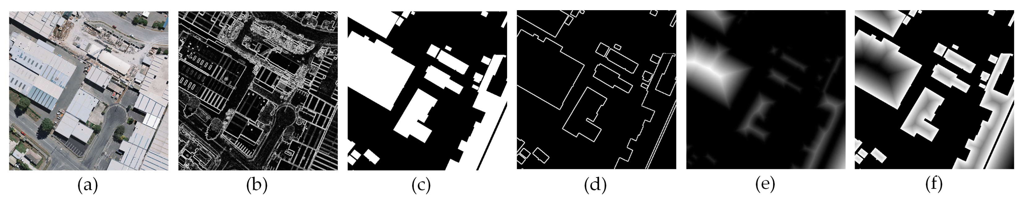
Firstly, we design a prior map generator to generate the segmentation maps and the inverse distance maps. These two maps are applied as prior information for the proposed GCCL module and GLFE module.

(2)

We propose a global context-constrained layer (GCCL), which effectively utilizes the prior knowledge to model high-quality features with global context constraints.

(3)

To enhance the semantic feature with local details, we propose the guided local feature enhancement block (GLFE), which obtains features with local texture context via a learnable guided filter from deeper layers.

(4)

To enhance the gradient consistency between the reconstructed HR image and the original HQ image, we develop a novel high-frequency consistency loss (HFC loss) by training a three-layer convolution neural network to simulate the canny boundary detection operator [23]. Then, the trained network is used as the loss network to enhance the high-frequency details of the reconstructed HR image.

The remainder of this paper is structured as follows: Section 2 presents the related work, Section 3 details the proposed CGC-Net, and Section 4 covers the experimental results, ablation studies, and our analysis. Finally, Section 5 concludes this work. In this paper, we use LQ, HQ, and HR to demonstrate the original low-quality image, ground-truth high-quality image, and reconstructed high-resolution image, respectively.

2. Related Work

2.1. Image Super-Resolution

A series of deep neural network-based methods have emerged in the field of SR in recent years due to the accelerating development of deep learning techniques. For instance, SRCNN [15] employs a three-layer convolution neural network to reconstruct high-resolution images. Although bicubic LR images outperform many conventional SR methods, such as SC [24], K-SVD [25], and ARN [26], they are computationally slow, causing a slow training speed. In order to solve this issue, the FSRCNN [27] and ESPCNN [28] methods send LR images directly to the network to extract features and learn HR feature maps. These methods reduce the reconstruction time of SRCNN [15] to 1/10 (ESPCNN [28])) and 1/38 (FSRCNN [27]), respectively.

Methods utilizing shallow network layers have a smaller receptive field. However, increasing the network’s depth affects its convergence and leads to gradient explosion or gradient disappearance [29] problems. Therefore, VDSR [30] integrates residual learning [31] to the SR field and applies adaptive gradient clipping to avoid gradient explosion [29] and deepen the model’s depth, strengthening the network’s hierarchical feature representation ability. Additionally, considering that the interpolation method in SRCNN [15] leads to reconstruction artifacts, the ESRCNN [32] method replaces interpolation with a sub-pixel convolution layer for upsampling. However, the simple shallow structure of ESRCNN [32] cannot easily learn the complex mapping between LR and HR images. Thus, Lai et al. designed LapSRN [33] (Laplacian Pyramid Networks for SR), a network structure based on the Laplacian pyramid model, to obtain a multilevel super-resolution map through the parameter sharing between modules and module cascaded step-by-step amplification.

However, CNN-based methods cannot distinguish and learn across feature channels, which limits the expression ability of the network. In addition to CNN-based methods, the self-attention mechanism and the Transformer [34] model have been gradually introduced into image SR tasks due to the powerful ability of sequence modeling and global information awareness. As the first attempt to use the attention mechanism on SR tasks, the residual channel attention network RCAN [35] adds the channel attention mechanism to the residual module, making it adaptively learn more useful channel features. Based on the Transformer [34] model, TTSR [36] uses the attention mechanism to recover the texture information of low-resolution images by learning the texture features of reference images.

2.2. Prior Knowledge-Based Image Super-Resolution

In recently reported review articles on image SR, most methods based on prior knowledge outperform traditional-based SR methods, which typically suffer from sharpening effects and difficulty in preserving details and textures.

To alleviate these problems, Yang et al. proposed a sparse coding-based image super-resolution method [24] that assumes high-resolution images can be represented as a linear combination of low-resolution images. Learning a K-dictionary [25] means the low-resolution images can be represented as a linear combination of sparse coefficients. Additionally, they incorporate regularization and L₂ parametric [37] minimization to ensure image sparsity. This approach employs dictionary learning to capture local features and achieves image SR. The core concept of this method is to create a sparse representation model that leverages small fragments of low-resolution images. Moreover, this method assumes that some local segments of high-resolution images can represent each of these fragments by utilizing L₂ parametric [37] minimization to obtain a sparse representation of each small fragment. This method effectively addresses the over-fitting issue in image SR, enhancing the model’s generalization ability. Subsequently, Liang et al. proposed SRCNN-Pr [38], which, combined with prior knowledge and the SRCNN [15], alleviated the problem of excessive parameters and reduced the network’s computational burden. However, achieving high-quality reconstruction of high-magnification images is still a challenge that SRCNN-Pr [38] needs to solve.

Previous works include edge-detection-based and edge-weighted-based super-resolution methods, which cannot recover the finer texture details. Although these methods enhance super-resolution results by introducing edge information, they have low edge detection accuracy and use ineffective edge-weighted strategies. To address these challenges, Chun et al. proposed SREdgeNet [39], a single-image SR method that enhances edges based on segmentation prior. This technique employs a dense edge detection network and a feature fusion network to enhance the SR effect. The edge detection network extracts the gradient features of the image, while the feature fusion network combines the edge information with the low-resolution features of the image to produce a high-resolution image.

2.3. Perceptual Loss

The effectiveness of MSE [40] and other pixel-wise loss functions in reconstructing high-frequency details of HR images is limited: minimizing MSE [40] encourages finding a pixel-averaged solution that is overly smooth and perceptually a poor result. Rather than pixel-wise loss, perceptual loss [41] compares the feature map obtained by HQ image convolution with the one obtained by HR image convolution to make the high-level information more consistent. The perceptual loss [41] comprises a trained loss network and loss functions, where the former extracts high-level semantic features, and the latter reduces the error between the feature maps extracted by the pre-trained loss network. Compared with the traditional comparison between the differences of individual pixels, the perceptual loss [41] can better retain higher levels of information on image SR tasks.

Numerous studies concentrate on designing loss functions with better-oriented texture learning ability. Extending from pixel-wise error measures, some researchers [42] measure the error from the features extracted from a pre-trained loss network. Perceptually more realistic SR results have been achieved by designing a loss function between feature maps extracted from the VGG network [43]. Subsequently, Li [44] studied the impact of patch comparison and mixing in the pixel and VGG feature spaces. However, existing perceptual loss methods do not consider semantic information when computing the reconstruction loss over the entire image. Recently, researchers have proposed a new method called SROBB [45], which generates object, background, and boundary (OBB) labels from segmentation labels to estimate the appropriate perceptual loss at the boundary. Additionally, SROBB [45] applies different penalties for images at different semantic levels.

Remote-sensing images usually not only cover the spectral information of multiple bands but also have a wealth of surface information. The traditional MSE [40] loss functions often make it difficult to retain the information accurately during overprocessing. However, a few perceptual loss [41] methods have been applied to remote sensing. To our knowledge, only Chen et al. advocated using semantic edge-aware loss [46] to improve remote-sensing segmentation precision.

3. Method

3.1. Overview of the Proposed Network

Figure 1 illustrates the proposed CGC-Net involving a simple encoder–decoder structure comprising five parts: prior maps generator, shallow content encoder, deep texture encoder, HR image reconstruction, and HFC Loss. The prior map generator includes a segmentation network (DeeplabV3+ [47] in this paper) and the inverse distance map generator. In a prior map generator, the low-quality (LQ) image $I_{LQ}\in {ℝ}^{H\times W\times C}$ (H, W, C are the image height, width, and the channel of the LQ image, respectively) is input into a segmentation network to obtain its segmentation map $I_{seg}\in {ℝ}^{H\times W\times C_1}$, and then from our carefully designed inverse distance transform, we generate the inverse distance map $I_{iv}\in {ℝ}^{H\times W\times C_1}$ from the segmentation map.

In the shallow content encoder, we use a simple convolutional layer to extract shallow features $F_l\in {ℝ}^{H\times W\times C_2}$ of the input LQ remote-sensing image, where the convolution layer provides a simple way to map the LQ image into higher-dimensional feature representations. Then, we extract deep features $F_d\in {ℝ}^{H\times W\times C_2}$ via the deep texture encoder, consisting of several global context-constrained layers (GCCL), guided local feature enhancement blocks (GLFE), and additional convolution layers. We input the LQ image with the segmentation map and the inverse distance map into the global context-constrained layer (GCCL) as prior knowledge to model the global contextual information of remote-sensing images. Although deeper layers focus on learning semantic representation [48], such networks lack learning local textures. Therefore, we design the guided local feature enhancement block (GLFE) to enhance the semantic features with local texture context. The additional convolution layer at the end of the deep texture encoder is designed to enhance the inductive bias, laying the foundation for the subsequent convergence of shallow and deep features.

At the end of the model, we use the sub-pixel convolution [17] as the high-resolution image reconstruction decoder to reconstruct the high-resolution (HR) remote-sensing image from aggregating shallow and deep features. In addition, we designed a novel high-frequency consistency (HFC Loss) to enhance the gradient consistency between the reconstructed HR image and the HQ image.

Section 3.2 introduces the proposed Prior Maps Generator. Section 3.3 and Section 3.4 present the global context-constrained layer (GCCL) and the guided local feature enhancement block (GLFE), and Section 3.5 introduces the loss functions.

3.2. Prior Maps Generator

Figure 1 depicts that the low-quality (LQ) remote-sensing image is first fed into a segmentation network (DeeplabV3+ [47]) to obtain the segmentation map. Next, we generate the inverse distance map via the inverse distance map generator. All processes for generating inverse distance maps are presented in Algorithm 1: Specifically, for one input segmentation map, p represents a pixel point inside the objects, and q is a pixel point on the object boundaries. Then, we calculate the distance between pixel point p and pixel point q using the Euclidean distance:

$$d(p,q)={‖p,q‖}_2$$

(1)

Furthermore, for every pixel point p, we define the transformation distance as:

$$D\left(p\right)=\underset{\forall q\in Q}{\min }\left(F(q)+d(p,q)\right)$$

(2)

where Q denotes the set of pixels on the object boundaries and $F(q)$ is the pixel value of point q. Then, we obtain the distance map $I_{\mathrm{dis}}$ by constantly updating the pixel values. Subsequently, we generate the inverse distance map by inverting the non-background region of the distance map. The result of the inverse distance map generator is illustrated in Figure 2.

Algorithm 1: Inverse Distance Map Generator

3.3. Global Contex-Constrained Layer (GCCL)

As shown in Figure 3, the proposed GCCL consists of a RSTB [17] and a constrained cross-attention block (CCAB). In GCCL, we input the LQ image with the segmentation map and the inverse distance map obtained from Section 3.2 as prior knowledge to model global contextual constraint information. Figure 2 highlights that the geometric context of images is well represented in the inverse distance map (Figure 2d), such as shape, boundary, and profile information. In addition, the segmentation map (Figure 2b) indicates the context of regions where pixels belonging to the same (different) class might have similar (different) textures in remote-sensing images. Therefore, we design a constrained cross-attention block (CCAB) in GCCL to use these maps as prior knowledge to learn high-quality features with global context constraints.

The workflow of CCAB is depicted in Figure 3b. We use the natural exponential function to smooth the value because there is a significant amount of zero entries in the segmentation map and the inverse distance map, as presented in Equations (3) and (4).

$$F_{seg}=\left(\exp \left(I_{seg}\right)-\min \left(\exp \left(I_{seg}\right)\right)\right)/\left(\max \left(\exp (I_{seg})\right)-\min \left(\exp \left(I_{seg}\right)\right)\right)$$

(3)

$$F_{iv}=\left(\exp \left(I_{iv}\right)-\min \left(\exp \left(I_{iv}\right)\right)\right)/\left(\max \left(\exp (I_{iv})\right)-\min \left(\exp \left(I_{iv}\right)\right)\right)$$

(4)

For convenience, we use $F_{seg}$ and $F_{iv}$ to demonstrate the tensor extracted from the normalized segmentation map and the inverse distance map, respectively. We use $F_{i-1}$ to demonstrate the tensor extracted from RSTB [17]. Specifically, we first calculate query (Q) from $F_{i-1}\in {ℝ}^{\widehat{H}\widehat{W}\times \widehat{C}}$ via a simple linear layer. Next, we apply element-wise multiplication between $F_{iv}\in {ℝ}^{\widehat{H}\times \widehat{W}\times C_i}$ and $F_{i-1}\in {ℝ}^{\widehat{H}\widehat{W}\times \widehat{C}}$. Then, the dot product $\widehat{F}\in {ℝ}^{\widehat{H}\widehat{W}\times \widehat{C}}$ is fed to another linear layer to get the value (V). Finally, we use a 3 × 3 convolution layer to extract the features of the segmentation map, and then we produce key (K) via another linear transformation. The process is described through the following equations:

$$Q=LN(F_{i-1})$$

(5)

$$K=LN\left(CONV\left(F_{seg}\right)\right)$$

(6)

$$V=LN(F_{iv}\odot F_{i-1})$$

(7)

where LN is the linear transform, and the CONV represents the convolution layer, while $\odot$ denotes element-wise multiplication. Finally, we calculate the constrained cross-attention value by applying the softmax function [49]. In addition, the input of CCAB is added to the output through the residual connection [31]. The overall process of CCAB is defined as follows:

$$\mathrm{Attention}(Q,K,V)=\mathrm{softmax}(Q{K}^{{\rm T}}/\sqrt{d_k})\cdot V$$

(8)

$$F_i=\mathrm{Attention}(Q,K,V)+F_{i-1}$$

(9)

where $d_k$ is the dimension of the query (Q), $F_{i-1}$ denotes the original input tensor, and $F_i$ represents the final output of GCCL. The Formula (8) is calculating the constrained cross-attention score. It is based on the calculation method of attention score proposed in Transformer [34] model. The formula 9 describes the process of residual connection, which is first proposed in Resnet [31]. Moreover, the coefficients are learned adaptively from the training data. The proposed CCAB borrows the ideas of Transformer [34] model.

3.4. Guided Local Feature Enhancement Block (GLFE)

As described in Section 3.3, the proposed CGC-Net models the global contextual constraint information from three GCCLs. Neural network with deeper layers has great ability on learning high-level features, while the ability of extracting low-level and local features is relatively weak [50]. Therefore, we propose a guided local feature enhancement block (GLFE) to enhance the local texture context via a learnable guided filter from deep layers. GLFE uses the Sobel gradient map of the segmentation map as the guided image (the guided image selection is studied in the experimental section) of a carefully designed guided filter layer while playing the key role in obtaining features with local texture context. The whole process of GLFE is depicted in Figure 4.

Figure 4 presents a feature map $I_f$, which is extracted from RSTB [17], as one of the input images of the guided filter layer. From the perspective of a guided filter, the high-frequency information of the output image $I_o$ is determined by the guided image. The developed scheme uses the Sobel Edge Detect operator [51] to create the segmentation map. Then, we use the Sobel gradient map of the segmentation map ${\mathrm{sobel}(I}_{\mathit{seg}})$ as the guided image (the choice of the guided image is studied in the experimental section) in the guided filter layer. Next, the output image is regarded as the local linear transformation of the guided image in the filtering window $w_k$. Thus, the output image can be expressed as:

$$I_o[i]=a_k\ast \left(\mathrm{sobel}\left(I_{seg}\right)[i]\right)+b_k,\forall i\in w_k$$

(10)

where $I_0[i]$ is the pixel value of the i-th point in the output image, $\mathrm{sobel}(I_{seg})[i]$ is the i-th point in the Sobel gradient map of the segmentation map, $a_k$ and $b_k$ are the linear coefficients of the local filtering window. This strategy has been proven useful in enhancing local details of the output image $I_o$.

To determine the linear coefficients, we assume that the noise between the output image $I_0$ and the input feature map $I_f$ is as small as possible. In addition, in the guided filter, a regularization parameter $ϵ$ is introduced to prevent $a_k$ from being too large. Thus, in the filtering window $w_k$, this purpose can be formulated as follows:

$$\arg \min {\displaystyle \sum _{i\in w_k}\left({\left(a_k\ast \left(\mathrm{sobel}(I_{seg})[i]\right)+b_k-I_f[i]\right)}^2+ϵa_k^2\right)}$$

(11)

Linear regression can give the optimization in Equation (11):

$$a_k=\frac{\frac{1}{\left|w\right|}{\displaystyle {\sum }_{i\in w_k}\left(\mathrm{sobel}\left(I_{seg}\right)[i]\ast I_f[i]\right)-{\mathsf{\mu }}_k\frac{1}{\left|w\right|}{\displaystyle {\sum }_{i\in w_k}{I}_f[i]}}}{{\sigma }_k^2+ϵ}$$

(12)

$$b_k=\frac{1}{\left|w\right|}{\displaystyle \sum _{i\in w_k}{I}_f}[i]-a_k{\mathsf{\mu }}_k$$

(13)

where ${\mathsf{\mu }}_k$ and ${\sigma }_k^2$ are the mean and variance of $\mathrm{sobel}(I_{seg})[i]$ in the filtering window $w_k$ and $\left|w\right|$ is the number of pixels in $w_k$. Then, by substituting the two linear coefficients into Equation (10), we can obtain the output of the guided filter [52]. In addition, in this module, we employ the residual connection [31]. Overall, the GLFE process is formulated as follows:

$$I_o=GF\left(I_f,\mathrm{sobel}\left(I_{seg}\right)\right)$$

(14)

$$F_o=I_f+I_o$$

(15)

where GF represents the guided filter, $I_f$ is the feature map extracted from RSTB [17], ${\mathrm{sobel}(I}_{\mathit{seg}})$ is the Sobel gradient map of the segmentation map, $I_o$ is the output of the guided filter layer, and $F_o$ is the final output of GLFE.

3.5. Loss Functions

High-frequency consistency loss (HFC loss). Unlike traditional perceptual loss [41], we design a novel high-frequency consistency loss (HFC loss) to measure the high-frequency information variance between the reconstructed HR images and the original HQ images. Specifically, we use the canny edge detector [23] to extract the high-frequency information of the image and then employ the canny gradient image as the true value to train a three-layer CNN network Ω (Figure 5a). Then, from the perspective of perceptual loss [41], Ω is considered a high-frequency loss network whose parameter is fixed while training the CGC-Net. In the HFC loss, we calculate the $L_1$ loss [29] between the feature maps of the reconstructed HR and HQ images while preserving their high-frequency consistency to enhance the high-frequency texture in the reconstructed HR image. The computational flow of HFC loss is illustrated in Figure 5b, and it can be formulated as follows:

$${\mathcal{L}}_{HFC}={\displaystyle \sum _i{\mathsf{\alpha }}_i{‖{\mathsf{\Omega }}_i(I_{HR})-{\mathsf{\Omega }}_i(I_{HQ})‖}_1}$$

(16)

where ${\mathsf{\Omega }}_i$ represents the i-th feature map of the high-frequency loss network and ${\mathsf{\alpha }}_i$ is the weight coefficient of this feature map, set to 1/4, 1/4, and 1/2, respectively.

Reconstruction loss. Considering that using $L_2$ loss [37] for reconstructing HR images will excessively smooth them, we adopt the $L_1$ loss [29] because it better maintains the spatial structure of the LQ images:

$${\mathcal{L}}_{rec}={‖I_{HR}-I_{HQ}‖}_1$$

(17)

Adversarial loss. To enhance the visual quality of the reconstructed image and restore its original texture, we utilize the adversarial loss from GAN [53]:

$${\mathcal{L}}_D={\displaystyle \sum _i\log }\left(1-D_{\eta }\left(G_{\theta }\left(x_i\right)\right)\right)$$

(18)

The total losses of the CGC-Net are as follows:

$$\mathcal{L}={\lambda }_1\ast {\mathcal{L}}_{rec}+{\lambda }_2\ast {\mathcal{L}}_D+{\lambda }_3\ast {\mathcal{L}}_{HFC}$$

(19)

where $\lambda$ represents the equilibrium parameter of each loss, set to 1, 0.2, and 0.04, respectively.

4. Experiments and Analysis

4.1. Datasets and Implementation Details

4.1.1. Datasets

In order to evaluate the effectiveness of our proposed model, we employ three challenging public remote-sensing image datasets, including the Inria Aerial Image dataset [54], the WHU Building dataset [55], and the ISPRS Potsdam dataset [56]. Several representative image samples are depicted in Figure 6.

The Inria Aerial Image dataset [54] consists of five open-access land-cover types from Chicago, Kitsap Country, Austin, Vienna, and West Tyrol. The images are aerial RGB with a very high spatial resolution of 0.3 m. There are 36 rectified images totaling 81 km² in each location. The dataset images are divided into 18,000 non-overlapping 500 × 500 tiles, and to decrease graphics memory requirements, we choose 120 images randomly and further crop them into 3000 smaller images, each measuring 100 × 100 pixels. The remaining images are utilized as the training set.

The WHU Building dataset [55] has 8189 image samples divided into building and non-building categories. A training set (4736 tiles), a test set (2416 tiles), and a validation set (1036 tiles) with a 512 × 512 size make up the 3 official divisions. Over 220,000 buildings from New Zealand are extracted for the WHU Building dataset [55], having the same spatial resolution of 0.3 m as the Inria Aerial Image dataset [54]. The dataset’s building labels are all artificially aligned. The 216 images used in our studies are randomly chosen, and the test set is split into 3456 smaller images with a 128 × 128 size. The remaining samples are used as the training set.

The 38 UAV remote-sensing images in the ISPRS Potsdam dataset [56] have a fixed resolution of 6000 × 6000 and generally fall into the following 6 categories: background, car, tree, low vegetation, building, and impervious surfaces. We divide these images into 5472 500 × 500 patches following earlier efforts. Then, 200 images are used as the test set, and 5272 images are randomly chosen as the training set. Additionally, the test set’s 200 images are divided into 3200 sub-images with a 100 × 100 size, which is used as the final test set to save graphics memory.

4.1.2. Implementation Details and Metrics

To generate low-quality (LQ) images with two, four, and eight sampling factors, the original high-quality (HQ) images are downsampled using the Bicubic function [29]. In order to evaluate the effectiveness of the proposed CGC-Net, we compare its performance with several classical SR methods (SRCNN [15], VDSR [30], EDSR [57], RCAN [35]), two of the latest state-of-the-art (SOTA) SR methods (SwinIR [17], Restormer [18]), and the specifically designed RSI-SR methods (MHAN [21], SA-GAN [58]). We employ two widely used image quality assessment metrics, namely PSNR and SSIM, to quantify the model’s performance. A larger PSNR value indicates a smaller distortion in the reconstructed HR image. The PSNR value can be calculated as follows:

$$PSNR=10{\log }_{10}\frac{MAX}{MSE}$$

(20)

where MAX is the maximum pixel value in the image, and the calculation formula of MSE is:

$$MSE=\frac{1}{HW}{\displaystyle \sum _{i=0}^{H-1}{\displaystyle \sum _{j=0}^{W-1}{\left[I_{HR}-I_{HQ}\right]}^2}}$$

(21)

where H and W represent the height and width of the image, respectively. Another full-reference index for evaluating image quality is SSIM, which evaluates image similarity based on brightness, contrast, and structure. The SSIM formula is:

$$SSIM(x,y)=l{(x,y)}^{\mathsf{\alpha }}c{(x,y)}^{\beta }s{(x,y)}^{\gamma }$$

(22)

However, the traditional image similarity measurement metrics are usually based on pixel value or structure information, which cannot reflect the difference in perception of human system vision. Therefore, to further demonstrate the effectiveness of our method, we also compare and evaluate the LPIPS value of each method. The LPIPS is calculated as:

$$LPIPS(x,y)=\frac{1}{n}{\displaystyle \sum _{i=1}^n{‖f_i(x)-f_i(y)‖}_2}$$

(23)

where x and y are the two images to be compared, $f_i$ represents the feature extractor of the i-th convolutional layer, and n represents the number of convolutional layers. All models are trained on a desktop with Ubuntu 22.04, CUDA 11.7, CUDNN 8.4, and two NVIDIA GTX 3090 GPUs. The Adam optimizer [37] is employed for optimization with β₁ = 0.9 and β₂ = 0.99. The learning rate is initialized to 2 × 10⁻⁴ and decreases based on a polygon learning rate adjustment schedule.

4.2. Comparison Experiments on the Inria Aerial Image Dataset

Table 1. SOTA comparisons on the Inria Aerial Image dataset [54]. The best and suboptimal results are shown in bold and underlined respectively.

Methods	Scales	PSNR↑	SSIM↑	LPIPS↓
SRCNN [15]		33.9729	0.8680	0.0963
VDSR [30]		34.1635	0.8710	0.0880
EDSR [57]		34.4402	0.8779	0.0800
RCAN [35]		34.4525	0.8782	0.0776
SwinIR [17]	×2	34.4400	0.8784	0.0831
Restormer [18]		34.4450	0.8787	0.0772
MHAN [21]		34.3525	0.8774	0.0783
SA-GAN [58]		34.3901	0.8777	0.0801
CGC-Net (Ours)		34.8202	0.8886	0.0715
SRCNN [15]		29.6069	0.7058	0.1787
VDSR [30]		29.6957	0.7110	0.1592
EDSR [57]		29.8370	0.7153	0.1401
RCAN [35]		29.8044	0.7141	0.1431
SwinIR [17]	×4	29.8411	0.7150	0.1409
Restormer [18]		29.8405	0.7009	0.1422
MHAN [21]		29.8212	0.7121	0.1410
SA-GAN [58]		29.8016	0.7119	0.1417
CGC-Net (Ours)		30.1717	0.7249	0.1376

shows the average performance of the proposed CGC-Net and other competing deep learning-based methods on the Inria Aerial Image dataset [54] with scale factors of 2 and 4. Bold values indicate the optimal outcomes and the underlined values are suboptimal. The proposed CGC-Net attains the best performance on the Inria Aerial Image dataset [54], achieving an average PSNR value of 0.3677/0.3306 dB, higher than the suboptimal method, for scale factors of 2 and 4, respectively. The mean SSIM values are 0.0099/0.0096 higher than the suboptimal method when the scale factors are 2 and 4, respectively. Furthermore, the mean LPIPS values are 0.0057/0.0025 lower than the suboptimal method when the scale factors are 2 and 4, respectively. It further demonstrates the effectives of our proposed CGC-Net method.

Figure 7 displays the reconstructed images from the other competing algorithms on the Inria Aerial Image dataset [54] with a scale factor of 2. Images in the third and fourth rows present the MSE maps between the reconstructed HR and the original HQ images. According to the reconstruction results, the proposed CGC-Net obtains superior PSNR/SSIM values than current approaches, which is also reflected in the MSE maps that present fewer errors (zoom in for a better view).

4.3. Comparison Experiments on the WHU Building Dataset

Table 2. SOTA comparisons on the WHU Building dataset [55]. The best and suboptimal results are shown in bold and underlined, respectively.

Methods	Scales	PSNR↑	SSIM↑	LPIPS↓
SRCNN [15]		25.7705	0.7119	0.1326
VDSR [30]		26.3692	0.7391	0.1124
EDSR [57]		26.7306	0.7531	0.1031
RCAN [35]		26.7347	0.7532	0.1030
SwinIR [17]	×2	26.7504	0.7543	0.1023
Restormer [18]		26.6706	0.7510	0.1048
MHAN [21]		26.7312	0.7533	0.1034
SA-GAN [58]		26.6692	0.7507	0.1051
CGC-Net (Ours)		27.0772	0.7615	0.1005
SRCNN [15]		22.8173	0.4857	0.2252
VDSR [30]		23.1390	0.5186	0.1932
EDSR [57]		23.5048	0.5464	0.1824
RCAN [35]		23.5346	0.5481	0.1818
SwinIR [17]	×4	23.5216	0.5468	0.1820
Restormer [18]		23.5754	0.5522	0.1804
MHAN [21]		23.5122	0.5466	0.1822
SA-GAN [58]		23.4817	0.5452	0.1841
CGC-Net (Ours)		24.0004	0.5626	0.1780

reports the performance comparison of CGC-Net and other deep learning-based methods on the WHU Building dataset [55] with scaling factors of 2 and 4. The optimal results are shown in bold, and the non-ideal results are underlined. The results infer that CGC-Net outperforms all competing methods on the WHU Building dataset [55]. Specifically, the mean PSNR value of CGC-Net is 0.3268/0.4250 dB, higher than the suboptimal method when the scale factors are 2 and 4, respectively. The mean SSIM values are 0.0072/0.0104 higher than those of the suboptimal method. Furthermore, the mean LPIPS values are 0.0018/0.0024 lower than those of the suboptimal method. A higher PSNR value indicates lower noise in the reconstructed image, while a higher SSIM value indicates less distortion in the reconstructed image. Additionally, a lower LPIPS value indicates the smaller the perceived distance between the reconstructed HR image and the original HQ image.

Figure 8 displays the reconstructed HR images of the WHU Building dataset [55] using various competitive methods with a scale factor of 2, demonstrating the same outcome. The third and fourth rows show the MSE maps between the original HQ and the reconstructed HR images. CGC-Net achieves better PSNR/SSIM values than the competitor deep learning-based SR methods, demonstrated by better recovering the textures and structures, such as clearer lines, in the reconstructed results. The MSE maps in the third and fourth rows also reflect fewer errors in our reconstructed HR image (zoom in for a better view).

4.4. Comparison Experiments on the ISPRS Potsdam Dataset

Furthermore, to evaluate the effectiveness of the proposed CGC-Net at higher amplification scale factors, we conduct a comparison study with several deep learning-based methods on the ISPRS Potsdam dataset [56]. In this study, we use scale factors of 4 and 8, which differs from those used in the other two datasets (2 and 4).

Table 3. SOTA comparisons on the ISPRS Potsdam dataset [56]. The best and suboptimal results are shown in bold and underlined, respectively.

Methods	Scales	PSNR↑	SSIM↑	LPIPS↓
SRCNN [15]		33.4417	0.8521	0.1206
VDSR [30]		34.1902	0.8645	0.1056
EDSR [57]		34.8442	0.8764	0.0944
RCAN [35]		34.8863	0.8784	0.0947
SwinIR [17]	×4	34.7476	0.8750	0.0951
Restormer [18]		34.8876	0.8789	0.0956
MHAN [21]		34.8246	0.8762	0.0960
SA-GAN [58]		34.6547	0.8709	0.0993
CGC-Net (Ours)		34.9884	0.8802	0.0898
SRCNN [15]		29.9821	0.7689	0.2151
VDSR [30]		30.2869	0.7787	0.1894
EDSR [57]		31.0672	0.7955	0.1727
RCAN [35]		31.0507	0.7953	0.1734
SwinIR [17]	×8	30.9103	0.7905	0.1751
Restormer [18]		31.0779	0.7994	0.1726
MHAN [21]		31.0501	0.7954	0.1732
SA-GAN [58]		31.0320	0.7948	0.1740
CGC-Net (Ours)		31.1674	0.7985	0.1729

reports the average performance of these methods, with bold values indicating optimal outcomes and underlined values representing suboptimal outcomes. Compared to the suboptimal method, the Restormer [18], CGC-Net shows higher average PSNR values of 0.1008/0.0895 dB with scale factors of 4 and 8, respectively. Similarly, when the scale factor is 4, CGC-Net exhibits a higher average SSIM of 0.0013 than Restormer [18]. In addition, CGC-Net exhibits a lower average LPIPS of 0.0046 than EDSR [57]. However, CGC-net shows larger SSIM values on the ×8 test set, mainly because the original spatial resolution is high, depressing the importance of learning the global and local constraint representations when the sampling ratio is high.

To better compare the reconstruction effect, we visualize the reconstructed high-resolution (HR) images on the ISPRS Potsdam dataset [56] with a scale factor of 4. The mean squared error (MSE) between the original high-quality (HQ) images and the reconstructed HR images is shown in the third and fourth rows of Figure 9. The suggested CGC-Net outperforms the competitor methods, as evidenced by the smaller reconstruction error highlighted in the red box (zoom in for a better view).

4.5. Model Efficiency Analysis

In order to evaluate the computational complexity of the proposed CGC-Net, we report the values of the model parameters (Params/M) and the floating-point operations per second (FLOPs) of these image super-resolution methods in

Table 4. Comparisons of model parameters (Params) and floating-point operations per second (FLOPs). Params and FLOPs are tested on a LR image with 48 × 48 pixels.

Method	Param (M)	FLOPs (G)
SRCNN [15]	0.06	0.26
VDSR [30]	0.67	1.53
EDSR [57]	40.72	4.75
RCAN [35]	15.44	35.36
SwinIR [17]	11.75	27.03
Restormer [18]	26.12	4.96
MHAN [21]	11.20	26.10
SA-GAN [58]	36.39	18.39
CGC-Net (Ours)	15.17	39.01

. The higher parameters indicate that the proposed CGC-Net has a stronger representation ability than the SwinIR [17] method. Combined with the floating-point operations per second (FLOPs) value of the proposed CGC-Net, it can be concluded that our method achieves a great trade-off between computational performance and model parameters. However, it also means higher computational cost and memory consumption of the CGC-Net. There is no doubt that this large computational complexity of the proposed CGC-Net leads to longer training time. In our feature studies, we will further optimize the computational complexity of the proposed CGC-Net.

4.6. Ablation Studies and Analysis

In this section, we ablate the importance of the elements involved in CGC-Net. All ablation results are conducted on the WHU Building dataset [55] with a scale factor of 2.

4.6.1. Hyperparameter Tuning of Weight Loss

This ablation study is conducted to determine the suitable setting for the weight loss. As described in Section 3.5, λ₁, λ₂, and λ₃ represent the weight coefficients of reconstruction loss, adversarial loss, and high-frequency consistency loss (HFC loss), respectively. Following previous works [59], we first experiment with the effect of only using reconstruction loss ${\mathcal{L}}_{rec}$, when λ₂ and λ₃ are set to 0. As shown in

Table 5. Results of average PSNR and SSIM values of different equilibrium parameters of each loss. The best and suboptimal results are shown in bold and underlined, respectively.

λ1	λ2	λ3	PSNR↑	SSIM↑
1	0	0	26.7891	0.7557
1	0.1	0.04	26.9293	0.7602
1	0.2	0.02	26.8841	0.7577
1	0.2	0.04	27.0772	0.7615

, when λ₂ and λ₃ are set to 0.1/0.04, an additional 0.1402 dB PSNR value and 0.0045 SSIM value can be obtained compared with only using reconstruction loss. However, when λ₂ and λ₃ are set to 0.2/0.02, a slight decrease of the PSNR/SSIM values can be observed. To obtain the best results, many hyperparameter adjustment experiments have been conducted, and we set the weight hyperparameters for reconstruction loss, adversarial loss, and HFC loss to 1, 0.2, 0.04, respectively. Due to the integral property of the Fourier transform [60], the weight of the proposed HFC loss is much less than other loss functions.

4.6.2. The Influence of Using Different Images as Guided Images

In this section, we investigate the impact of utilizing various images, such as the low-quality (LQ) image, the Sobel gradient map of the LQ image, the segmentation map, the Sobel gradient map of the segmentation map, the distance map, and the inverse distance map, as guided images in guided local feature enhancement block (GLFE). The guided filter assigns high-frequency information to the output image based on the guided image, influencing the overall SR results. Figure 10 illustrates the different guided image representations.

Table 6. The effect of using different images as guided images on the performance of the model in guided local feature enhancement block (GLFE). The bold represents the best value for each metric, and the upward arrow indicates that the larger the value is, the better the performance.

Guided Image	PSNR↑	SSIM↑
LQ image	26.7858	0.7559
the gradient map of LQ image	26.7906	0.7561
Segmentation map	26.7379	0.7541
the gradient map of the segmentation map	27.0772	0.7615
distance map	26.7388	0.7543
inverse distance map	26.7440	0.7543

reports the most optimal results achieved when utilizing the gradient map of the segmentation map as the guided image. Conversely, unsatisfactory performance is observed when using the LQ image and its gradient map. Deeper layers focus on learning a semantic representation [48], while lacking learning local textures. Due to the global characteristics of the LQ image and its Sobel gradient map, the model fails to focus on the local objective textures effectively. Since the segmentation map approximates the attention map, driving the model pays more attention to the local textures that need to be restored, explicitly enhancing local textures. The local information in the segmentation, distance, and inverse distance maps are redundant, resulting in unsatisfactory results.

4.6.3. Components Ablations

In order to showcase the efficacy of the individual components, we progressively incorporated the global context-constrained layer (GCCL), the guided local feature enhancement block (GLFE), the high-frequency consistency loss (HFC loss), and GAN loss into the baseline model. We trained all models with the same configuration, and the corresponding results per metric are presented in

Table 7. The effect of incrementally adding different components on model performance compared to the baseline model. GCCL represents the global contextual constraint layer, GLFE represents guided local feature enhancement block, HFC Loss represents high-frequency consistency loss. Bold text indicates the optimal value for each metric.

Baseline	GCCL	GLFE	HFC Loss	GAN Loss	PSNR↑	SSIM↑
✓	✗	✗	✗	✗	25.7745	0.7120
✓	✓	✗	✗	✗	26.5934	0.7480
✓	✓	✓	✗	✗	26.7891	0.7557
✓	✓	✓	✓	✗	26.9291	0.7600
✓	✓	✓	✓	✓	27.0772	0.7615

. Additionally, Figure 11 displays the visualization images.

Table 7 demonstrates that including additional modules results in a gradual improvement of the PSNR and SSIM values. The developed CGC-Net exhibits the best performance when all modules are incorporated, as the proposed guided context-constrained layer (GCCL) increases the PSNR values to 0.8189 dB and the SSIM values to 0.0360 SSIM values compared to the baseline model. Next, adding the guided local feature enhancement block (GLFE) significantly improves PSNR/SSIM to 0.1957 dB/0.0077, respectively. An additional 0.1400 dB PSNR value and 0.0043 SSIM value can be obtained via our carefully designed high-frequency consistency loss (HFC Loss). Furthermore, applying GAN Loss has a minor positive impact on the result, demonstrating that all modules are indispensable for the proposed CGC-Net.

Figure 11 reveals that the reconstruction effect of the baseline model is blurry. After adding GCCL, the lines in the playground are clearer, while GLFE increases the information detail. After adding our carefully designed HFC loss, the lines in the playground and the roads are more accurate. Finally, by adding GAN Loss, the reconstruction HR image obtains the best visual performance.

4.6.4. CGC-Net with Different Training Scales

In this section, we investigate the adaptability of the proposed CGC-Net to a different number of training labels. We divide the WHU Building dataset [55] into a training set and a test set according to different partition ratios of 8:2, 5:5, and 2:8, respectively. As shown in

Table 8. The adaptability of the proposed CGC-Net to different numbers of training labels. The best and suboptimal results are shown in bold and underlined, respectively.

Partition Ratio	Model	PSNR↑	SSIM↑
	RCAN [35]	26.6043	0.7530
training set/test set	MHAN [21]	26.5778	0.7528
(8:2)	SwinIR [17]	26.6201	0.7532
	CGC-Net (Ours)	26.9438	0.7591
	RCAN [35]	26.4044	0.7503
training set/test set	MHAN [21]	26.4001	0.7493
(5:5)	SwinIR [17]	26.4079	0.7504
	CGC-Net (Ours)	26.5021	0.7506
	RCAN [35]	26.2502	0.7394
training set/test set	MHAN [21]	26.2379	0.7388
(2:8)	SwinIR [17]	26.2505	0.7396
	CGC-Net (Ours)	26.3376	0.7401

, when the dataset partition ratio is 8:2, the mean PSNR/SSIM values are 0.3237 dB/0.0059 higher than the SwinIR [17] model. This is mainly because sufficient training samples enable CGC-Net to make full use of the target information in prior maps. Especially, to evaluate the performance of the proposed CGC-Net on small labels, we divide a smaller training set according to the dataset partition ration of 2:8. Experimental results still show greater performance of the proposed CGC-Net compared to the other models. It can be observed from Table 8 that our proposed method achieves consistent performance improvements on all training scales.

4.6.5. Adaptability to Noise

To further demonstrate the progressiveness of the proposed CGC-Net, we study the adaptability of the proposed algorithm to image noise. As a common experimental setup in the literature [61], additional Gaussian noises [62] with zero mean and standard deviation σ are added to images to test the performance of noise adaptability. In this paper, noise level σ are set as 10, 30, and 50, respectively. Figure 12 shows the test images with different noise levels. SRCNN [15], VDSR [30], EDSR [57], RCAN [35], SwinIR [17], Restormer [18], MHAN [21], and SA-GAN [58] are compared. As shown in

Table 9. Average PSNR and SSIM results of σ 10, 30, 50 on WHU Building dataset [55]. The best and suboptimal results are shown in bold and underlined, respectively.

	$\sigma =10$	$\sigma =30$	$\sigma =50$
	PSNR↑
SRCNN [15]	25.0205	22.8105	21.6805
VDSR [30]	25.6692	23.5392	22.4392
EDSR [57]	26.0402	23.9402	22.7402
RCAN [35]	25.9947	23.9647	22.7747
SwinIR [17]	26.0404	23.9104	22.7804
Restormer [18]	25.9606	23.7906	22.5906
MHAN [21]	26.0312	23.8812	22.7112
SA-GAN [58]	25.9392	23.8392	22.7092
CGC-Net (Ours)	26.3672	24.0672	22.9772
	SSIM↑
SRCNN [15]	0.6714	0.4851	0.3927
VDSR [30]	0.6944	0.5489	0.4197
EDSR [57]	0.7353	0.5900	0.4570
RCAN [35]	0.7352	0.5991	0.4569
SwinIR [17]	0.7359	0.5975	0.4591
Restormer [18]	0.7350	0.5910	0.4483
MHAN [21]	0.7354	0.5913	0.4585
SA-GAN [58]	0.7342	0.5879	0.4555
CGC-Net (Ours)	0.7442	0.6029	0.4665

, the mean PSNR/SSIM values of the proposed CGC-Net are 0.3268 dB/0.0083, 0.1025 dB/0.0038, and 0.1968 dB/0.0074 higher than the suboptimal results when the noise level σ is 10, 30, 50, respectively. The experimental results demonstrate that the proposed CGC-Net has better robustness and generalization ability compared to other models.

4.6.6. Lower and Upper Boundaries of the Proposed CGC-Net

This section investigates the impact of directly utilizing Ground Truth prior maps (including the segmentation map and the inverse distance map), prior maps predicted by the DeeplabV3+ [47] model, and random noise maps on the performance of CGC-Net. These different map representations are depicted in Figure 13.

Table 10. The influence of utilizing different prior maps on the performance of CGC-Net. The best results are shown in bold.

Prior Maps	PSNR↑	SSIM↑
Ground Truth	27.1979	0.7619
DeeplabV3+ [47]	27.0772	0.7615
Random noise map	26.5379	0.7401

reveals that using Ground Truth prior maps achieves the best PSNR/SSIM values, our model’s upper boundary. Our method uses the DeeplabV3+ [47] model to generate the segmentation map and then generates the inverse distance map. This method achieves 27.0772/0.7615 PSNR/SSIM values. Using random noise maps achieves unsatisfactory results because disorganized noise points disable the model from learning effective information. Thus, we assume that the results of using random noise maps are the lower boundary of our model.

4.6.7. The Influence of Different Reconstructed HR Datasets on Segmentation Task

This study examines the impact of super-resolution reconstruction on downstream tasks by reconstructing the WHU Building dataset [55] using different SR methods. Specifically, we use datasets with varying resolutions to assess the segmentation performance of the segformer [63] model. The mean intersection over union (mIoU) and mean accuracy (mAcc) are used as standard evaluation metrics to assess the performance of the segmentation model. The mIOU metric calculates the average ratio of the intersection and union between two images (ground truth and expected outcome), and mACC represents the average forecast accuracy per category. All segmentation experiments are conducted under the same parameters to ensure a fair comparison.

Table 11. The influence of WHU Building dataset [55] reconstructed by different SR methods with a scale factor of 2 on the downstream segmentation task. All segmentation experimental results are based on segformer [63] model. The best and suboptimal results are shown in bold and underlined, respectively.

Datasets	IoU (%)		Acc (%)		mIoU (%)	mAcc (%)
	Building	Clutter	Building	Clutter
SRCNN (HR) [15]	86.09	98.47	89.97	99.52	92.28	94.75
VDSR (HR) [30]	86.91	98.54	91.46	99.44	92.72	95.45
EDSR (HR) [57]	87.46	98.60	92.45	99.39	93.03	95.92
RCAN (HR) [35]	87.61	98.63	91.90	99.48	93.12	95.69
SwinIR (HR) [17]	88.18	98.69	92.21	99.51	93.44	95.86
Restormer (HR) [18]	87.89	98.66	92.21	99.48	93.27	95.84
CGC-Net (Ours HR)	89.47	98.83	93.84	99.48	94.15	96.66

highlights that the dataset reconstructed by the proposed CGC-Net achieves the best mIoU and mAcc values, presenting the best SR results compared to the competitor methods. Due to the unsatisfactory reconstruction effect of the SRCNN [15] method, the results of segformer [63] model on this dataset are also unsatisfying. Combined with the reconstruction performance of each method, Table 7 infers that the performance of the segmentation model is positively correlated with the resolution of the reconstructed image. Figure 14 demonstrates that the segformer [63] model achieves better results on the dataset reconstructed by CGC-Net. Hence, the local areas are visualized much better, strongly demonstrating the significance of the SR algorithm in improving the performance of downstream tasks.

5. Conclusions

This paper proposes a novel Context-Guided Constrained Network, named CGC-Net for remote-sensing image super-resolution. In CGC-Net, we first design a simple but effective method to generate inverse distance maps from the remote-sensing image segmentation maps as prior information. Combined with prior information, we propose a Global Context-Constrained layer (GCCL). In GCCL, we employ the characteristics of the segmentation map and the inverse distance map to model high-quality features with global context constraints. Furthermore, we introduce a Guided Local Feature Enhancement Block (GLFE) to enhance local texture context via a learnable guided filter from deeper layers. Additionally, we design a High-Frequency Consistency loss (HFC Loss) to balance the gradient consistency between the reconstructed HR image and the original HQ image. Compared with competitive deep learning-based methods, the experimental results demonstrate promising SR performance from CGC-Net on three typical remote-sensing image datasets. The reconstructed HR datasets of the proposed CGC-Net achieve state-of-the-art (SOTA) results on downstream image segmentation tasks, strongly demonstrating the potential of super-resolution (SR) algorithm to boost the performance of downstream tasks.

References

1. Sishodia, R.P.; Ray, R.L.; Singh, S.K. Applications of Remote Sensing in Precision Agriculture: A Review. Remote Sens. 2020, 12, 3136. [Google Scholar] [CrossRef]
2. Majumdar, S. The Role of Remote Sensing and GIS in Military Strategy to Prevent Terror Attacks. Intell. Data Anal. Terror. Threat. Predict. Archit. Methodol. Tech. Appl. 2021, 14, 79–94. [Google Scholar]
3. Yang, L.; Shi, L.; Sun, W.; Yang, J.; Li, P.; Li, D.; Liu, S.; Zhao, L. Radiometric and Polarimetric Quality Validation of Gaofen-3 over a Five-Year Operation Period. Remote Sens. 2023, 15, 1605. [Google Scholar] [CrossRef]
4. Giovos, R.; Tassopoulos, D.; Kalivas, D.; Lougkos, N.; Priovol, A. Remote Sensing Vegetation Indices in Viticulture: A Critical Review. Agriculture 2021, 11, 457. [Google Scholar] [CrossRef]
5. Shimoni, M.; Haelterman, R.; Perneel, C. Hypersectral Imaging for Military and Security Applications: Combining Myriad Processing and Sensing Techniques. IEEE Geosci. Remote Sens. Mag. 2019, 7, 101–117. [Google Scholar] [CrossRef]
6. Zhu, Q.; Zhen, L.; Zhang, Y.; Guan, Q. Building Extraction from High Spatial Resolution Remote Sensing Images via Multiscale-Aware and Segmentation-Prior Conditional Random Fields. Remote Sens. 2020, 12, 3983. [Google Scholar] [CrossRef]
7. Zhang, L.; Dong, R.; Yuan, S.; Li, W.; Zheng, J.; Fu, H. Making Low-Resolution Satellite Images Reborn: A Deep Learning Approach for Super-Resolution Building Extraction. Remote Sens. 2021, 13, 2872. [Google Scholar] [CrossRef]
8. Schuegraf, P.; Bittner, K. Automatic Building Footprint Extraction from Multi-Resolution Remote Sensing Images Using a Hybrid FCN. ISPRS Int. J. Geo-Inf. 2019, 8, 191. [Google Scholar] [CrossRef] [Green Version]
9. Zeng, Y.; Guo, Y.; Li, J. Recognition and extraction of high-resolution satellite remote sensing image buildings based on deep learning. Neural Comput. Appl. 2022, 34, 2691–2706. [Google Scholar] [CrossRef]
10. Dong, Z.; Wang, M.; Wang, Y.; Zhu, Y.; Zhang, Z. Object Detection in High Resolution Remote Sensing Imagery Based on Convolutional Neural Networks With Suitable Object Scale Features. IEEE Trans. Geosci. Remote Sens. 2020, 58, 2104–2114. [Google Scholar] [CrossRef]
11. Su, Y.; Wu, Y.; Wang, M.; Wang, F.; Cheng, J. Semantic Segmentation of High Resolution Remote Sensing Image Based on Batch-Attention Mechanism. In IEEE International Geoscience and Remote Sensing Symposium; IEEE: Piscataway, NJ, USA, 2019. [Google Scholar]
12. Guo, Z.; Wu, G.; Song, X.; Yuan, W.; Chen, Q.; Zhang, H.; Shi, X.; Xu, M.; Xu, Y.; Shibasaki, R.; et al. Super-Resolution Integrated Building Semantic Segmentation for Multi-Source Remote Sensing Imagery. IEEE Access 2019, 7, 99381–99397. [Google Scholar] [CrossRef]
13. Ding, Y.; Zhang, Z.; Zhao, X.; Cai, W.; Yang, N.; Hu, H.; Yuan, C.; Cai, W. Unsupervised Self-Correlated Learning Smoothy Enhanced Locality Preserving Graph Convolution Embedding Clustering for Hyperspectral Images. TGRS 2022, 60. [Google Scholar] [CrossRef]
14. Zhang, J.; Xu, T.; Li, J.; Jiang, S.; Zhang, Y. Single-Image Super Resolution of Remote Sensing Images with Real-World Degradation Modeling. Remote Sens. 2022, 14, 2895. [Google Scholar] [CrossRef]
15. Dong, C.; Loy, C.C.; He, K.; Tang, X. Image Super-Resolution Using Deep Convolutional Networks. IEEE Trans. Pattern Anal. Mach. Intell. 2014, 38, 295–307. [Google Scholar] [CrossRef] [Green Version]
16. Liu, Z.; Lin, Y.; Cao, Y.; Hu, H.; Wei, Y.; Zhang, Z.; Lin, S.; Guo, B. Swin Transformer: Hierarchical Vision Transformer using Shifted Windows. arXiv 2021, arXiv:2103.14030. [Google Scholar]
17. Liang, J.; Cao, J.; Sun, G.; Zhang, K.; Gool, L.V.; Timofte, R. SwinIR: Image Restoration Using Swin Transformer. In Proceedings of the IEEE/CVF International Conference on Computer Vision (ICCV) Workshops, Montreal, BC, Canada, 11–17 October 2021. [Google Scholar]
18. Zamir, S.W.; Arora, A.; Khan, S.; Hayat, M.; Khan, F.S.; Yang, M.H. Restormer: Efficient Transformer for High-Resolution Image Restoration. In Proceedings of the IEEE/CVF Conference on Computer Vision and Pattern Recognition (CVPR), New Orleans, LA, USA, 18–24 June 2022. [Google Scholar]
19. Ding, Y.; Zhang, Z.; Zhao, X.; Hong, D.; Wei, C.; Yang, N.; Wang, B. Multi-scale receptive fields: Graph attention neural network for hyperspectral image classification. Expert Syst. Appl. 2023, 223, 119858. [Google Scholar] [CrossRef]
20. Zhang, Z.; Ding, Y.; Zhao, X.; Siye, L.; Yang, N.; Cai, Y.; Zhan, Y. Multireceptive field: An adaptive path aggregation graph neural framework for hyperspectral image classification. Expert Syst. Appl. 2023, 217, 119508. [Google Scholar] [CrossRef]
21. Zhang, D.; Shao, J.; Li, X.; Shen, H. Remote Sensing Image Super-Resolution via Mixed High-Order Attention Network. IEEE Trans. Geosci. Remote Sens. 2021, 59, 5183–5196. [Google Scholar] [CrossRef]
22. Wang, J.; Shao, Z.; Huang, X.; Lu, T. From Artifact Removal to Super-Resolution. IEEE Trans. Geosci. Remote Sens. 2022, 60. [Google Scholar] [CrossRef]
23. Canny, J. A Computational Approach to Edge Detection. IEEE Trans. Pattern Anal. Mach. Intell. 1987, PAMI-8, 679–698. [Google Scholar] [CrossRef]
24. Yang, J.; Wright, J.; Huang, W.S.; Ma, Y. Image Super-Resolution Via Sparse Representation. IEEE Trans. Image Process. 2010, 19, 2861–2873. [Google Scholar] [CrossRef] [PubMed]
25. Aharon, M.; Elad, M.; Bruckstein, A. K-SVD: An algorithm for designing overcomplete dictionaries for sparse representation. IEEE Trans. Signal Process. 2006, 54, 4311–4322. [Google Scholar] [CrossRef]
26. Zhang, Y.; Sun, L.; Yan, C.; Ji, X.; Dai, Q. Adaptive Residual Networks for High-Quality Image Restoration. IEEE Trans. Image Process. 2018, 27, 3150–3163. [Google Scholar] [CrossRef] [PubMed]
27. Dong, C.; Loy, C.; Tang, X. Accelerating the super-resolution convolutional neural network. In Proceedings of the Computer Vision–ECCV 2016: 14th European Conference, Amsterdam, The Netherlands, 11–14 October 2016. [Google Scholar]
28. Shi, W.; Caballero, J.; Huszár, F.; Totz, J.; Aitken, A.P.; Bishop, R.; Rueckert, D.; Wang, Z. Real-Time Single Image and Video Super-Resolution Using an Efficient Sub-Pixel Convolutional Neural Network. In Proceedings of the IEEE Conference on Computer Vision and Pattern Recognition (CVPR), Las Vegas, NV, USA, 27–30 June 2016. [Google Scholar]
29. BenGio, Y.; Simard, P.; Fransconi, P. Learning Long-Term Dependencies with Gradient Descent is Difficult. IEEE Trans. Neural Netw. 1994, 5, 157–166. [Google Scholar] [CrossRef] [PubMed]
30. Kim, J.; Lee, J.K.; Lee, K.M. Accurate Image Super-Resolution Using Very Deep Convolutional Networks. In Proceedings of the IEEE Conference on Computer Vision and Pattern Recognition, Las Vegas, NV, USA, 27–30 June 2016; pp. 1646–1654. [Google Scholar]
31. He, K.; Zhang, X.; Ren, S.; Sun, J. Deep Residual Learning for Image Recognition. In Proceedings of the IEEE Conference on Computer Vision and Pattern Recognition (CVPR), Las Vegas, NV, USA, 27–30 June 2016. [Google Scholar]
32. Jung, Y.; Choi, Y.; Sim, J.; Kim, L. eSRCNN: A Framework for Optimizing Super-Resolution Tasks on Diverse Embedded CNN Accelerators. In Proceedings of the IEEE/ACM International Conference on Computer-Aided Design, Westminster, CO, USA, 4–7 November 2019. [Google Scholar]
33. Lai, W.; Huang, J.; Ahuja, N.; Yang, M. Deep Laplacian Pyramid Networks for Fast and Accurate Super-Resolution. In Proceedings of the IEEE Conference on Computer Vision and Pattern Recognition (CVPR), Honolulu, HI, USA, 21–27 July 2017. [Google Scholar]
34. Vaswani, A.; Shazeer, N.; Parmar, N.; Uszkoreit, J.; Jones, L.; Gomez, A.N.; Lukasz, K.; Polosukhin, L. Attention Is All You Need. arXiv. Adv. Neural Inf. Process. Syst. 2017, 30. [Google Scholar] [CrossRef]
35. Zhang, Y.; Li, K.; Wang, L.; Zhong, B.; Fu, Y. Image Super-Resolution Using Very Deep Residual Channel Attention Networks. In Proceedings of the European Conference on Computer Vision (ECCV), Munich, Germany, 8–14 September 2018. [Google Scholar]
36. Yang, F.; Yang, H.; Fu, J.; Lu, H.; Guo, B. Learning Texture Transformer Network for Image Super-Resolution. In Proceedings of the IEEE/CVF Conference on Computer Vision and Pattern Recognition, Seattle, WA, USA, 13–19 June 2020. [Google Scholar]
37. Loshchilov, I.; Hutter, F. Decoupled Weight Decay Regularization. In Proceedings of the International Conference on Learning Representations (ICLR), Toulon, France, 24–26 April 2017. [Google Scholar]
38. Liang, J.; Wang, J.; Zhou, S.; Gong, Y.; Zheng, N. Incorporating image priors with deep convolutional neural networks for image super-resolution. Neurocomputing 2016, 194, 340–347. [Google Scholar] [CrossRef] [Green Version]
39. Kim, K.; Chun, S.Y. SREdgeNet: Edge Enhanced Single Image Super Resolution using Dense Edge Detection Network and Feature Merge Network. arXiv 2018, arXiv:1812.07174. [Google Scholar]
40. Wang, Z.; Bovik, A.C.; Sheikh, H.R.; Simoncelli, E.P. Image quality assessment: From error visibility to structural similarity. IEEE Trans. Image Process. 2004, 13, 600–612. [Google Scholar] [CrossRef] [Green Version]
41. Johnson, J.; Alahi, A.; Li, F. Perceptual Losses for Real-Time Style Transfer and Super-Resolution. In Proceedings of the Computer Vision—ECCV 2016, Amsterdam, The Netherlands, 11–14 October 2016. [Google Scholar]
42. Bruna, J.; Sprechmann, P.; LeCun, Y. Super-Resolution with Deep Convolutional Sufficient Statistics. arXiv 2016, arXiv:1511.05666. [Google Scholar]
43. Li, C.; Wand, M. Precomputed Real-Time Texture Synthesis with Markovian Generative Adversarial Networks. In Proceedings of the Computer Vision—ECCV 2016, Amsterdam, The Netherlands, 11–14 October 2016. [Google Scholar]
44. Li, C.; Wand, M. Combining Markov Random Fields and Convolutional Neural Networks for Image Synthesis. In Proceedings of the IEEE Conference on Computer Vision and Pattern Recognition (CVPR), Las Vegas, NV, USA, 27–30 June 2016. [Google Scholar]
45. Rad, M.S.; Bozorgtabar, B.; Marti, U.; Basler, M.; Ekenel, H.; Thiran, J. SROBB: Targeted Perceptual Loss for Single Image Super-Resolution. In Proceedings of the IEEE/CVF International Conference on Computer Vision (ICCV), Seoul, Republic of Korea, 27 October–2 November 2019. [Google Scholar]
46. Chen, Y.; Dapogny, A.; Cord, M. SEMEDA: Enhancing Segmentation Precision with Semantic Edge Aware Loss. Pattern Recognit. 2019, 108, 107557. [Google Scholar] [CrossRef]
47. Chen, L.; Zhu, Y.; Papandreou, G.; Schoroff, F.; Adam, H. Encoder-Decoder with Atrous Separable Convolution for Semantic Image Segmentation. arXiv 2018, arXiv:1802.02611. [Google Scholar]
48. Saha, S.; Obukhov, A.; Paudel, D.; Kanakis, M.; Chen, Y.; Georgoulis, S.; Gool, L. Learning to Relate Depth and Semantics for Unsupervised Domain Adaptation. arXiv 2021, arXiv:2105.07830. [Google Scholar]
49. Liu, W.; Wen, Y.; Yu, Z.; Yang, M. Large-Margin Softmax Loss for Convolutional Neural Networks. arXiv 2016, arXiv:1612.02295. [Google Scholar]
50. Schoenholz, S.S.; Gilmer, J.; Ganguli, S.; Sohl-Dickstein, J. Deep Information Propagation. arXiv 2016. [Google Scholar] [CrossRef]
51. Zhang, Y.; Han, X.; Zhang, H.; Zhao, L. Edge detection algorithm of image fusion based on improved Sobel operator. In Proceedings of the IEEE 3rd Information Technology and Mechatronics Engineering Conference, Chongqing, China, 3–5 October 2017. [Google Scholar]
52. He, K.; Sun, J.; Tang, X. Guided Image Filtering. IEEE Trans. Pattern Anal. Mach. Intell. 2012, 35, 1397–1409. [Google Scholar] [CrossRef]
53. Goodfellow, L.J.; Pouget-Abadie, J.; Mirza, M.; Xu, B.; Warde-Farley, D.; Ozair, S.; Courville, A.; Bengio, Y. Generative Adversarial Networks. IEEE Signal Process. Mag. 2018, 35, 53–65. [Google Scholar] [CrossRef]
54. Maggiori, E.; Tarabalka, Y.; Charpiat, G.; Alliez, P. Can semantic labelling methods generalize to any city? The inria aerial image labelling benchmark. In Proceedings of the 2017 IEEE International Geoscience and Remote Sensing Symposium (IGARSS), Fort Worth, TX, USA, 23–28 July 2017; pp. 3226–3229. [Google Scholar]
55. Ji, S.; Wei, S.; Lu, M. Fully Convolutional Networks for Multisource Building Extraction From an Open Aerial and Satellite Imagery Data Set. IEEE Trans. Geosci. Remote Sens. 2018, 574, 574–586. [Google Scholar] [CrossRef]
56. ISPRS Potsdam 2D Semantic Labeling Dataset. Available online: https://www.isprs.org/education/benchmarks/UrbanSemLab/2d-sem-label-potsdam.aspx (accessed on 15 December 2022).
57. Lim, B.; Son, S.; Kim, H.; Nah, S.; Lee, K.M. Enhanced Deep Residual Networks for Single Image Super-Resolution. arXiv 2017, arXiv:1707.02921. [Google Scholar]
58. Zhao, J.; Ma, Y.; Chenm, F.; Shang, E.; Yao, W.; Zhang, S.; Yang, J. SA-GAN: A Second Order Attention Generator Adversarial Network with Region Aware Strategy for Real Satellite Images Super Resolution Reconstruction. Remote Sens. 2023, 15, 1391. [Google Scholar] [CrossRef]
59. Zhang, Z.; Wang, Z.; Lin, Z.L.; Qi, H. Image Super-Resolution by Neural Texture Transfer. In Proceedings of the IEEE/CVF Conference on Computer Vision and Pattern Recognition (CVPR), Long Beach, CA, USA, 15–20 June 2019; pp. 7974–7983. [Google Scholar]
60. Healy, D.J. Fast Fourier transforms for Nonequispaced Data. SIAM J. Sci. Comput. 1998, 19, 529–545. [Google Scholar]
61. Mao, X.; Shen, C.; Yang, Y. Image Restoration Using Convolutional Auto-encoders with Symmetric Skip Connections. arXiv 2016, arXiv:1606.08921. [Google Scholar]
62. Portilla, J.; Strela, V.; Wainwright, M.J.; Simoncelli, E.P. Imageenoising using scale mixtures of Gaussians in the wavelet domain. IEEE Trans. Image Process. 2003, 12, 1338–1351. [Google Scholar] [CrossRef] [PubMed] [Green Version]
63. Xie, E.; Wang, W.; Yu, Z.; Anandkumar, A.; Alvarez, J.M.; Luo, P. SegFormer: Simple and Efficient Design for Semantic Segmentation with Transformers. Adv. Neural Inf. Process. Syst. 2021, 34, 12077–12090. [Google Scholar]
Figure 1. The architecture of the proposed model for remote-sensing image super resolution. Our model follows the simple encoder–decoder architecture. The core modules of the model are: (a) Inverse Distance Map Generator that uses the segmentation map to generate the inverse distance map. (b) Global Context-Constrained Layer (GCCL) that uses the segmentation map and the inverse distance map in cross-attention to enhance global features. (c) Guided Local Feature Enhancement Block (GLFE) that uses the gradient map of the segmentation map as the guided image in the guided filter layer to enhance local features. (d) High-frequency Consistency Loss (HFC Loss) that enhances the gradient consistency between the reconstructed HR image and the HQ image. denotes element-wise addition.
Remotesensing 15 03171 g001
Figure 2. One example is input LQ image with different output representations. (a) Low-Quality Image (RGB), (b) Semantic Segmentation Map, (c) Distance Map, (d) Inverse Distance Map.
Remotesensing 15 03171 g002
Figure 3. The structure of the proposed GCCL. (a) Two components of GCCL. (b) The workflow of the proposed constrained cross-attention block (CCAB). LN and CONV stand for linear layer and convolution layer respectively.
Remotesensing 15 03171 g003
Figure 4. The calculation process of the guided local feature enhancement block (GLFE). denotes ele-ment-wise addition.
Remotesensing 15 03171 g004
Figure 5. The proposed HFC loss for gradient consistency. (a) The training process of HFC loss network. (b) The computational flow of HFC loss.
Remotesensing 15 03171 g005
Figure 6. Close-up images of three datasets. The image samples in the Inria Aerial image dataset [54], the WHU Building dataset [55], and the ISPRS Potsdam dataset [56] are shown from the first to the third row, correspondingly.
Remotesensing 15 03171 g006
Figure 7. A visual comparison of the proposed CGC-Net with other models on the Inria Aerial Image dataset [54]. The models were evaluated using a scale factor of 2, and the third and fourth rows of the figure show the mean squared error (MSE) between the high-quality (HQ) image and the high-resolution (HR) results.
Remotesensing 15 03171 g007
Figure 8. A visual comparison of the proposed CGC-Net with other models on the WHU Building dataset [55]. The models were evaluated using a scale factor of 2, and the third and fourth rows of the figure show the mean squared error (MSE) between the high-quality (HQ) image and the high-resolution (HR) results.
Remotesensing 15 03171 g008
Figure 9. A visual comparison of the proposed CGC-Net with other models on the ISPRS Potsdam dataset [56]. The models were evaluated using a scale factor of 4, and the third and fourth rows of the figure show the mean squared error (MSE) between the high-quality (HQ) image and the high-resolution (HR) results.
Remotesensing 15 03171 g009
Figure 10. One example using different images as the guided image. (a) LQ image, (b) The Sobel gradient map of LQ image, (c) Segmentation map, (d) The Sobel gradient map of the segmentation map, (e) Distance map, and (f) Inverse distance map.
Remotesensing 15 03171 g010
Figure 11. The overall visual comparisons show the impact of each module on the reconstruction effect.
Remotesensing 15 03171 g011
Figure 12. Test images with different noise level σ of 10, 30, and 50, respectively.
Remotesensing 15 03171 g012
Figure 13. Different representations of the prior maps. Building: white, and clutter: black.
Remotesensing 15 03171 g013
Figure 14. Mapping results on the WHU Building dataset [55] reconstructed by different SR methods. Building: white and clutter: black.
Remotesensing 15 03171 g014