
Sharp Feature-Preserving 3D Mesh Reconstruction from Point Clouds Based on Primitive Detection

Abstract
:1. Introduction
- We propose a novel complete framework for reconstructing meshes from point clouds based on primitive detection. Our framework can accurately preserve sharp and clear boundary features and generate high-fidelity reconstruction models.
- The framework includes an improved learning-based primitive detection module. Experiments show that it outperforms previous methods, with Seg-IoU and Type-IoU scores improving from to . In addition, we specifically designed a refine submodule to optimize the detected segmentation, obtaining more reasonable segmentation patches.
- The framework also includes an efficient module for mesh splitting that can separate overlapping meshes at the triangle level, producing clear and continuous segmentation blocks. This module helps our framework reconstruct high-quality sharp edges, and it can be well parallelized.
- Our framework also features a novel optimization selection module, which treats the reconstruction task as a minimum subset selection problem. In our framework, this module is responsible for selecting the optimal subset from the already split mesh collection, to obtain the optimal reconstruction result. The design of this module considers both the local and global information of the input model.
2. Related Work
2.1. Surface Reconstruction
2.1.1. Non-Learning-Based Methods
2.1.2. Learning Based Methods
2.2. Primitive Detection
2.2.1. Non-Learning-Based Methods
2.2.2. Learning-Based Methods
3. Method
3.1. Primitive Detection Module
3.1.1. Coarse Primitive Detection Based on Supervised Learning
3.1.2. Refine Clustering via Normal Angle
3.2. Mesh Fitting and Splitting Module
3.3. Selection Module
3.3.1. Energy Terms
3.3.2. Optimization
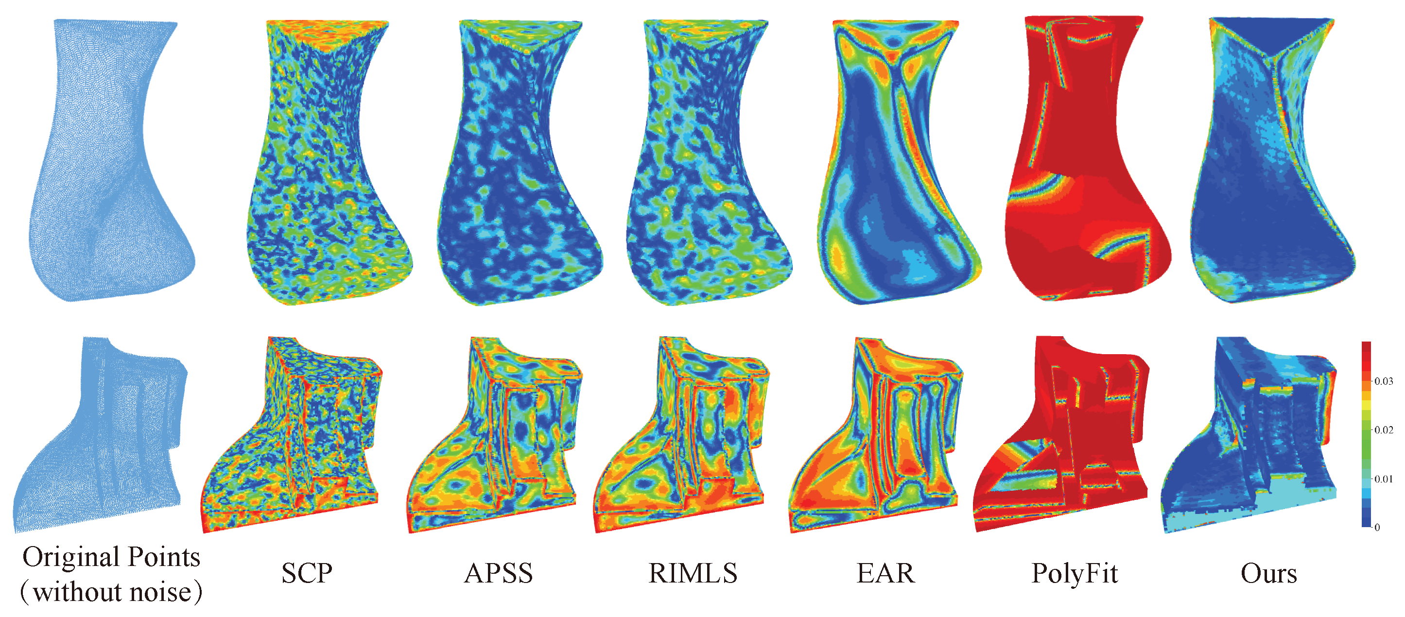
4. Results
4.1. Datasets
4.2. Experiment Details and Results Analysis
- Seg-IoU: this metric measures the similarity between the predicted patches and ground truth segments: , where W is the predicted segmentation membership for each point cloud, is the ground truth, and K is the number of ground truth segments.
- Type-IoU: this metric measures the classification accuracy of primitive type prediction: , where is the predicted primitive type for the kth segment patch and is the ground truth. is an indicator function.
- Throughput: this metric measures the efficiency performance of the network: ins./sec., meaning maximum number of instances the network can handle per second.
4.3. Exploratory Experiments
5. Conclusions
Author Contributions
Funding
Data Availability Statement
Acknowledgments
Conflicts of Interest
References
- Berger, M.; Tagliasacchi, A.; Seversky, L.M.; Alliez, P.; Guennebaud, G.; Levine, J.A.; Sharf, A.; Silva, C.T. A Survey of Surface Reconstruction from Point Clouds. Comput. Graph. Forum 2017, 36, 301–329. [Google Scholar] [CrossRef] [Green Version]
- Berger, M.; Tagliasacchi, A.; Seversky, L.M.; Alliez, P.; Levine, J.a.; Sharf, A.; Silva, C.T.; Tagliasacchi, A.; Seversky, L.M.; Silva, C.T.; et al. State of the Art in Surface Reconstruction from Point Clouds. In Proceedings of the 35th Annual Conference of the European Association for Computer Graphics, Eurographics 2014-State of the Art Reports (No. CONF), Strasbourg, France, 7–11 April 2014; Volume 1, pp. 161–185. [Google Scholar]
- Kaiser, A.; Ybanez Zepeda, J.A.; Boubekeur, T. A Survey of Simple Geometric Primitives Detection Methods for Captured 3D Data. Comput. Graph. Forum 2019, 38, 167–196. [Google Scholar] [CrossRef]
- Fischler, M.A.; Bolles, R.C. Random Sample Consensus: A Paradigm for Model Fitting with Applications to Image Analysis and Automated Cartography. In Readings in Computer Vision; Fischler, M.A., Firschein, O., Eds.; Morgan Kaufmann: San Francisco, CA, USA, 1987; pp. 726–740. [Google Scholar] [CrossRef]
- Schnabel, R.; Wahl, R.; Klein, R. Efficient RANSAC for point-cloud shape detection. Comput. Graph. Forum 2007, 26, 214–226. [Google Scholar] [CrossRef]
- Yan, D.M.; Wang, W.; Liu, Y.; Yang, Z. Variational mesh segmentation via quadric surface fitting. CAD Comput. Aided Des. 2012, 44, 1072–1082. [Google Scholar] [CrossRef]
- Lafarge, F.; Mallet, C. Creating large-scale city models from 3D-point clouds: A robust approach with hybrid representation. Int. J. Comput. Vis. 2012, 99, 69–85. [Google Scholar] [CrossRef] [Green Version]
- Li, L.; Sung, M.; Dubrovina, A.; Yi, L.; Guibas, L.J. Supervised fitting of geometric primitives to 3D point clouds. In Proceedings of the IEEE Computer Society Conference on Computer Vision and Pattern Recognition, Long Beach, CA, USA, 16–20 June 2019; pp. 2647–2655. [Google Scholar] [CrossRef] [Green Version]
- Sharma, G.; Liu, D.; Maji, S.; Kalogerakis, E.; Chaudhuri, S.; Měch, R. ParSeNet: A Parametric Surface Fitting Network for 3D Point Clouds. Lect. Notes Comput. Sci. 2020, 12352, 261–276. [Google Scholar] [CrossRef]
- Yan, S.; Yang, Z.; Ma, C.; Huang, H.; Vouga, E.; Huang, Q. HPNet: Deep Primitive Segmentation Using Hybrid Representations. In Proceedings of the IEEE/CVF International Conference on Computer Vision, Montreal, QC, Canada, 11–17 October 2021. [Google Scholar] [CrossRef]
- Lorensen, W.E.; Cline, H.E. Marching Cubes: A High Resolution 3D Surface Construction Algorithm. SIGGRAPH Comput. Graph. 1987, 21, 163–169. [Google Scholar] [CrossRef]
- Alexa, M.; Behr, J.; Cohen-Or, D.; Fleishman, S.; Levin, D.; Silva, C.T. Computing and rendering point set surfaces. IEEE Trans. Vis. Comput. Graph. 2003, 9, 3–15. [Google Scholar] [CrossRef] [Green Version]
- Wang, H.; Scheidegger, C.E.; Silva, C.T. Bandwidth selection and reconstruction quality in point-based surfaces. IEEE Trans. Vis. Comput. Graph. 2009, 15, 572–582. [Google Scholar] [CrossRef] [Green Version]
- Carr, J.C.; Beatson, R.K.; Cherrie, J.B.; Mitchell, T.J.; Fright, W.R.; McCallum, B.C.; Evans, T.R. Reconstruction and representation of 3D objects with radial basis functions. In Proceedings of the 28th Annual Conference on Computer Graphics and Interactive Techniques, SIGGRAPH 2001, Los Angeles, CA, USA, 12–17 August 2001; pp. 67–76. [Google Scholar] [CrossRef]
- Brazil, E.V.; Macedo, I.; Sousa, M.C.; de Figueiredo, L.H.; Velho, L. Sketching Variational Hermite-RBF Implicits. In Proceedings of the Seventh Sketch-Based Interfaces and Modeling Symposium, Annecy, France, 7–10 June 2010; SBIM ’10. pp. 1–8. [Google Scholar]
- Huang, Z.; Carr, N.; Ju, T. Variational implicit point set surfaces. ACM Trans. Graph. 2019, 38, 124. [Google Scholar] [CrossRef]
- Kazhdan, M.; Bolitho, M.; Hoppe, H. Poisson Surface Reconstruction. In Proceedings of the Fourth Eurographics Symposium on Geometry Processing, Sardinia, Italy, 26–28 June 2006; SGP ’06. pp. 61–70. [Google Scholar]
- Kazhdan, M.; Hoppe, H. Screened poisson surface reconstruction. ACM Trans. Graph. 2013, 32, 29. [Google Scholar] [CrossRef] [Green Version]
- Fleishman, S.; Cohen-Or, D.; Silva, C.T. Robust moving least-squares fitting with sharp features. ACM Trans. Graph. 2005, 24, 544–552. [Google Scholar] [CrossRef] [Green Version]
- Öztireli, A.C.; Guennebaud, G.; Gross, M. Feature Preserving Point Set Surfaces based on Non-Linear Kernel Regression. Comput. Graph. Forum 2009, 28, 493–501. [Google Scholar] [CrossRef] [Green Version]
- Huang, H.; Wu, S.; Gong, M.; Cohen-Or, D.; Ascher, U.; Zhang, H.R. Edge-aware point set resampling. ACM Trans. Graph. 2013, 32, 9. [Google Scholar] [CrossRef]
- Lipman, Y.; Cohen-Or, D.; Levin, D.; Tal-Ezer, H. Parameterization-free projection for geometry reconstruction. In Proceedings of the ACM SIGGRAPH Conference on Computer Graphics, San Diego, CA, USA, 5–9 August 2007. [Google Scholar] [CrossRef] [Green Version]
- Chen, Z.; Zhang, H. Learning Implicit Fields for Generative Shape Modeling. In Proceedings of the IEEE Conference on Computer Vision and Pattern Recognition (CVPR), Long Beach, CA, USA, 15–20 June 2019. [Google Scholar]
- Park, J.J.; Florence, P.; Straub, J.; Newcombe, R.; Lovegrove, S. DeepSDF: Learning Continuous Signed Distance Functions for Shape Representation. In Proceedings of the The IEEE Conference on Computer Vision and Pattern Recognition (CVPR), Long Beach, CA, USA, 15–20 June 2019. [Google Scholar]
- Mescheder, L.; Oechsle, M.; Niemeyer, M.; Nowozin, S.; Geiger, A. Occupancy Networks: Learning 3D Reconstruction in Function Space. In Proceedings of the IEEE Conference on Computer Vision and Pattern Recognition (CVPR), Long Beach, CA, USA, 15–20 June 2019. [Google Scholar]
- Erler, P.; Guerrero, P.; Ohrhallinger, S.; Mitra, N.J.; Wimmer, M. Points2Surf: Learning Implicit Surfaces from Point Clouds. In Proceedings of the Computer Vision—ECCV 2020, Glasgow, UK, 23–28 August 2020; pp. 108–124. [Google Scholar] [CrossRef]
- Jiang, C.M.; Sud, A.; Makadia, A.; Huang, J.; Nießner, M.; Funkhouser, T. Local Implicit Grid Representations for 3D Scenes. In Proceedings of the IEEE Conference on Computer Vision and Pattern Recognition (CVPR), Seattle, WA, USA, 13–19 June 2020. [Google Scholar]
- Songyou, P.; Michael, N.; Lars, M.; Marc, P.; Andreas, G. Convolutional Occupancy Networks. In Proceedings of the European Conference on Computer Vision (ECCV), Glasgow, UK, 23–28 August 2020. [Google Scholar]
- Schnabel, R.; Degener, P.; Klein, R. Completion and reconstruction with primitive shapes. Comput. Graph. Forum 2009, 28, 503–512. [Google Scholar] [CrossRef]
- Lafarge, F.; Alliez, P. Surface reconstruction through point set structuring. Comput. Graph. Forum 2013, 32, 225–234. [Google Scholar] [CrossRef] [Green Version]
- Nan, L.; Wonka, P. PolyFit: Polygonal Surface Reconstruction from Point Clouds. In Proceedings of the IEEE International Conference on Computer Vision, Venice, Italy, 22–29 October 2017; pp. 2372–2380. [Google Scholar] [CrossRef] [Green Version]
- Sharma, G.; Goyal, R.; Liu, D.; Kalogerakis, E.; Maji, S. CSGNet: Neural Shape Parser for Constructive Solid Geometry. In Proceedings of the IEEE Computer Society Conference on Computer Vision and Pattern Recognition, Salt Lake City, UT, USA, 18–23 June 2018; pp. 5515–5523. [Google Scholar] [CrossRef] [Green Version]
- Yu, F.; Chen, Z.; Li, M.; Sanghi, A.; Shayani, H.; Mahdavi-Amiri, A.; Zhang, H. CAPRI-Net: Learning Compact CAD Shapes with Adaptive Primitive Assembly. In Proceedings of the IEEE/CVF Conference on Computer Vision and Pattern Recognition, Nashville, TN, USA, 20–25 June 2021. [Google Scholar] [CrossRef]
- Wang, Y.; Sun, Y.; Liu, Z.; Sarma, S.E.; Bronstein, M.M.; Solomon, J.M. Dynamic Graph CNN for Learning on Point Clouds. ACM Trans. Graph. 2019, 38, 146. [Google Scholar] [CrossRef] [Green Version]
- Comaniciu, D.; Meer, P. Mean shift: A robust approach toward feature space analysis. IEEE Trans. Pattern Anal. Mach. Intell. 2002, 24, 603–619. [Google Scholar] [CrossRef] [Green Version]
- Qian, G.; Li, Y.; Peng, H.; Mai, J.; Hammoud, H.; Elhoseiny, M.; Ghanem, B. PointNeXt: Revisiting PointNet++ with Improved Training and Scaling Strategies. In Advances in Neural Information Processing Systems; Koyejo, S., Mohamed, S., Agarwal, A., Belgrave, D., Cho, K., Oh, A., Eds.; Curran Associates, Inc.: Red Hook, NY, USA, 2022; Volume 35, pp. 23192–23204. [Google Scholar]
- Qi, C.R.; Yi, L.; Su, H.; Guibas, L.J. PointNet++: Deep Hierarchical Feature Learning on Point Sets in a Metric Space. In Proceedings of the 31st International Conference on Neural Information Processing Systems, Long Beach, CA, USA, 4–9 December 2017; NIPS’17; pp. 5105–5114. [Google Scholar]
- Ma, X.; Qin, C.; You, H.; Ran, H.; Fu, Y. Rethinking Network Design and Local Geometry in Point Cloud: A Simple Residual MLP Framework. In Proceedings of the International Conference on Learning Representations, Virtual Event, 25–29 April 2022. [Google Scholar]
- Zhao, H.; Jiang, L.; Jia, J.; Torr, P.H.; Koltun, V. Point Transformer. In Proceedings of the IEEE/CVF International Conference on Computer Vision (ICCV), Montreal, QC, Canada, 10–17 October 2021; pp. 16259–16268. [Google Scholar]
- Sandler, M.; Howard, A.; Zhu, M.; Zhmoginov, A.; Chen, L.C. MobileNetV2: Inverted Residuals and Linear Bottlenecks. In Proceedings of the 2018 IEEE/CVF Conference on Computer Vision and Pattern Recognition, Salt Lake City, UT, USA, 18–23 June 2018; pp. 4510–4520. [Google Scholar] [CrossRef] [Green Version]
- Lu, X.; Yao, J.; Tu, J.; Li, K.; Li, L.; Liu, Y. Pairwise linkage for point cloud segmentation. ISPRS Ann. Photogramm. Remote Sens. Spat. Inf. Sci. 2016, 3, 201–208. [Google Scholar] [CrossRef] [Green Version]
- Alliez, P.; Giraudot, S.; Jamin, C.; Lafarge, F.; Mérigot, Q.; Meyron, J.; Saboret, L.; Salman, N.; Wu, S.; Yildiran, N.F. Point Set Processing. In CGAL User and Reference Manual, 4th ed; CGAL Editorial Board: New York, NY, USA, 2022. [Google Scholar]
- Kettner, L.; Meyer, A.; Zomorodian, A. Intersecting Sequences of dD Iso-oriented Boxes. In CGAL User and Reference Manual, 3rd ed; CGAL Editorial Board: New York, NY, USA, 2021. [Google Scholar]
- Nan, L.; Sharf, A.; Zhang, H.; Cohen-Or, D.; Chen, B. SmartBoxes for interactive urban reconstruction. In ACM Siggraph 2010 Papers, Siggraph 2010; ACM: New York, NY, USA, 2010. [Google Scholar] [CrossRef]
- Gurobi Optimization, LLC. Gurobi Optimizer Reference Manual. 2021. Available online: https://www.gurobi.com (accessed on 27 April 2023).
- Zhou, Q.; Jacobson, A. Thingi10K: A Dataset of 10, 000 3D-Printing Models. arXiv 2016, arXiv:abs/1605.04797. [Google Scholar]
- Koch, S.; Matveev, A.; Williams, F.; Alexa, M.; Zorin, D.; Panozzo, D.; Files, C.A.D. ABC: A Big CAD Model Dataset For Geometric Deep Learning. arXiv 2019, arXiv:1812.06216v2. [Google Scholar]
- Wang, X.; Xu, Y.; Xu, K.; Tagliasacchi, A.; Zhou, B.; Mahdavi-Amiri, A.; Zhang, H. PIE-NET: Parametric Inference of Point Cloud Edges. Adv. Neural Inf. Process. Syst. 2020, 33, 20167–20178. [Google Scholar]
- Kuhn, H.W. The Hungarian method for the assignment problem. Nav. Res. Logist. Q. 1955, 2, 83–97. [Google Scholar] [CrossRef] [Green Version]
- Bernardini, F.; Mittleman, J.; Rushmeier, H.; Silva, C.; Taubin, G. The Ball-Pivoting Algorithm for Surface Reconstruction. IEEE Trans. Vis. Comput. Graph. 1999, 5, 349–359. [Google Scholar] [CrossRef]
- Loshchilov, I.; Hutter, F. Decoupled Weight Decay Regularization. In Proceedings of the ICLR, New Orleans, LA, USA, 6–9 May 2019. [Google Scholar]
- Szegedy, C.; Vanhoucke, V.; Ioffe, S.; Shlens, J.; Wojna, Z. Rethinking the Inception Architecture for Computer Vision. In Proceedings of the 2016 IEEE Conference on Computer Vision and Pattern Recognition (CVPR), Las Vegas, NV, USA, 27–30 June 2016; pp. 2818–2826. [Google Scholar] [CrossRef] [Green Version]
- Kingma, D.P.; Ba, J. Adam: A Method for Stochastic Optimization. arXiv 2014, arXiv:1412.6980. [Google Scholar]
- Guennebaud, G.; Gross, M. Algebraic point set surfaces. In Proceedings of the ACM SIGGRAPH Conference on Computer Graphics, San Diego, CA, USA, 5–9 August 2007. [Google Scholar] [CrossRef]
- Cignoni, P.; Callieri, M.; Corsini, M.; Dellepiane, M.; Ganovelli, F.; Ranzuglia, G. MeshLab: An Open-Source Mesh Processing Tool. In Proceedings of the Eurographics Italian Chapter Conference, Salerno, Italy, 2–4 July 2008; Scarano, V., Chiara, R.D., Erra, U., Eds.; The Eurographics Association: Crete, Greece, 2008. [Google Scholar] [CrossRef]
- Chandra, R.; Dagum, L.; Kohr, D.; Menon, R.; Maydan, D.; McDonald, J. Parallel Programming in OpenMP; Morgan Kaufmann: Burlington, MA, USA, 2001. [Google Scholar]
- Mérigot, Q.; Ovsjanikov, M.; Guibas, L.J. Voronoi-based curvature and feature estimation from point clouds. IEEE Trans. Vis. Comput. Graph. 2011, 17, 743–756. [Google Scholar] [CrossRef] [Green Version]
- Zhuang, Y.; Zou, M.; Carr, N.; Ju, T. Anisotropic geodesics for live-wire mesh segmentation. Comput. Graph. Forum 2014, 33, 111–120. [Google Scholar] [CrossRef] [Green Version]


| Method | Seg-IoU (%) | Type-IoU (%) | Throughput (ins./sec.) |
|---|---|---|---|
| SPFN [8] | 73.41 | 80.04 | 21 |
| ParSeNet [9] | 82.14 | 88.6 | 8 |
| HPNet [10] | 85.24 | 91.04 | 8 |
| Ours | 88.42 | 92.85 | 28 |
| Improvements | Seg-IoU (%) | Type-IoU (%) | Throughput (ins./sec.) |
|---|---|---|---|
| Baseline (HPNet [10]) | 85.24 | 91.04 | 8 |
| +DGCNN [34] → PointNeXt-b [36] | 86.88 | 92.23 | 28 |
| +Adam [53] → AdamW [51] | 87.34 | 92.74 | 28 |
| +Step → Cosine | 87.50 | 92.67 | 28 |
| +Label Smoothing [52] | 88.42 | 92.85 | 28 |
| Vase | Fandisk | |||
|---|---|---|---|---|
| Faces. | Sec. | Faces. | Sec. | |
| Screened Possion [18] | 9996 | 1.98 | 40,028 | 3.08 |
| APSS [54] | 9996 | 1.59 | 17,815 | 4.34 |
| RIMLS [20] | 9996 | 2.41 | 17,801 | 6.63 |
| EAR [21] | 181,170 | 128.98 | 272,593 | 202.39 |
| PolyFit [31] | 38 | 1.81 | 17 | 3.39 |
| Ours | 4068 | 7.92 | 6403 | 69.09 |
| Ours + OpenMP [56] | 4068 | 2.26 | 6403 | 7.35 |
| Method | Vase | Fandisk | ||||||
|---|---|---|---|---|---|---|---|---|
| Shortest dis. ( mm) | Hausdorff dis. ( mm) | Mean dis. ( mm) | Median dis. ( mm) | Shortest dis. ( mm) | Hausdorff dis. ( mm) | Mean dis. ( mm) | Median dis. ( mm) | |
| Screened Possion [18] | 27.35 | 8.014 | 1.766 | 1.390 | 117.8 | 20.24 | 2.983 | 2.572 |
| APSS [54] | 149.0 | 5.579 | 1.120 | 0.897 | 26.28 | 19.32 | 3.051 | 2.806 |
| RIMLS [20] | 31.28 | 5.663 | 1.296 | 1.022 | 97.25 | 19.86 | 3.515 | 3.303 |
| EAR [21] | 8.227 | 10.57 | 1.647 | 1.152 | 197.7 | 19.95 | 3.843 | 3.575 |
| PolyFit [31] | 3525 | 210.7 | 53.52 | 36.32 | 1586 | 260.4 | 45.34 | 31.94 |
| Ours | 0.003 | 8.132 | 1.499 | 1.343 | 15.82 | 18.85 | 1.162 | 1.008 |
Disclaimer/Publisher’s Note: The statements, opinions and data contained in all publications are solely those of the individual author(s) and contributor(s) and not of MDPI and/or the editor(s). MDPI and/or the editor(s) disclaim responsibility for any injury to people or property resulting from any ideas, methods, instructions or products referred to in the content. |
© 2023 by the authors. Licensee MDPI, Basel, Switzerland. This article is an open access article distributed under the terms and conditions of the Creative Commons Attribution (CC BY) license (https://creativecommons.org/licenses/by/4.0/).
Share and Cite
Liu, Q.; Xu, S.; Xiao, J.; Wang, Y. Sharp Feature-Preserving 3D Mesh Reconstruction from Point Clouds Based on Primitive Detection. Remote Sens. 2023, 15, 3155. https://doi.org/10.3390/rs15123155
Liu Q, Xu S, Xiao J, Wang Y. Sharp Feature-Preserving 3D Mesh Reconstruction from Point Clouds Based on Primitive Detection. Remote Sensing. 2023; 15(12):3155. https://doi.org/10.3390/rs15123155
Chicago/Turabian StyleLiu, Qi, Shibiao Xu, Jun Xiao, and Ying Wang. 2023. "Sharp Feature-Preserving 3D Mesh Reconstruction from Point Clouds Based on Primitive Detection" Remote Sensing 15, no. 12: 3155. https://doi.org/10.3390/rs15123155