Article

Influence of On-Site Camera Calibration with Sub-Block of Images on the Accuracy of Spatial Data Obtained by PPK-Based UAS Photogrammetry

Geomatics Department, Federal University of Paraná, Curitiba 81531-990, Brazil
*
Author to whom correspondence should be addressed.
Remote Sens. 2023, 15(12), 3126; https://doi.org/10.3390/rs15123126
Submission received: 6 April 2023 / Revised: 16 May 2023 / Accepted: 16 May 2023 / Published: 15 June 2023

Abstract

:
Unmanned Aerial Systems (UAS) Photogrammetry has become widely used for spatial data acquisition. Nowadays, RTK (Real Time Kinematic) and PPK (Post Processed Kinematic) are the main correction methods for accurate positioning used for direct measurements of camera station coordinates in UAS imagery. Thus, 3D camera coordinates are commonly used as additional observations in Bundle Block Adjustment to perform Global Navigation Satellite System-Assisted Aerial Triangulation (GNSS-AAT). This process requires accurate Interior Orientation Parameters to ensure the quality of photogrammetric intersection. Therefore, this study investigates the influence of on-site camera calibration with a sub-block of images on the accuracy of spatial data obtained by PPK-based UAS Photogrammetry. For this purpose, experiments of on-the-job camera self-calibration in the Metashape software with the SfM approach were performed. Afterward, experiments of GNSS-Assisted Aerial Triangulation with on-site calibration in the Erdas Imagine software were performed. The outcomes show that only the experiment of GNSS-AAT with three Ground Control Points yielded horizontal and vertical accuracies close to nominal precisions of the camera station positions by GNSS-PPK measurements adopted in this study, showing horizontal RMSE (Root-Mean Square Error) of 0.222 m and vertical RMSE of 0.154 m. Furthermore, the on-site camera calibration with a sub-block of images significantly improved the vertical accuracy of the spatial information extraction.

1. Introduction

Unmanned Aerial Systems (UAS), regularly referred to as Unmanned Aerial Vehicles (UAVs) or Remotely Piloted Aircraft Systems (RPAS) [1], have become widely used for spatial data acquisition. In the last decade, the use of UAS has received considerable emphasis in environmental applications, such as the investigation of active volcanos and lava movement [2,3], quantification of soil loss and erosion [4,5,6], landslide monitoring [7,8,9], structural geology studies [10,11] and observation of glaciological movements [12,13]. Positional accuracy and precision are highly relevant for applications focused on Geoscience. Thus, several studies aim to validate and improve the accuracy of spatial data obtained with UAS [14,15]. The quality of three-dimensional information obtained by UAS imagery depends on several factors [14,15,16], such as the number and distribution of Ground Control Points (GCPs) [17,18,19,20], overlap between images [15,21], camera calibration method [22,23], flight configuration [24,25], and processing software [26,27].
Compared to the manned aircraft used in conventional photogrammetric surveys, UAS has a lower operating cost, greater ease of use, and automation of the process [16]. Furthermore, due to the low flight altitude, UAS usage enables the generation of high-resolution terrain models even when equipped with low-cost cameras [28]. However, the use of UAS is still limited to smaller areas, as the flight autonomy of small UAS is commonly less than 30 min [29,30]. Another disadvantage lies in the platform stability, which is more affected by temporal conditions and can interfere with image overlap [31]. Furthermore, as UAS-acquired images are obtained at considerably lower altitudes than those typically used in conventional photogrammetry, they exhibit characteristics similar to those observed in close-range photogrammetric applications, such as increased perspective distortions, as well as wide variations in lighting and scale across images [5,32]. As a result, another essential factor to be considered in achieving accurate UAS Photogrammetric surveys is the variation in surface height relative to the flight altitude.
Traditionally, GCPs are required to perform Indirect Sensor Orientation of the camera via Bundle Block Adjustment (BBA), i.e., Aerial Triangulation. However, in regions that are difficult to access, such as dense vegetation areas and glacial zones, it usually becomes very costly to perform the field survey [23,30]. Moreover, surveying points coordinates on the ground can offer risks to human health in geohazard monitoring, such as the occurrence of wildfires, volcanic activity, and earthquakes [33,34]. In this context, reducing or eliminating the need for GCPs is desirable. With the development of increasingly smaller sensors over the past decade, GNSS (Global Navigation Satellite System) receivers and high-accuracy INS (Inertial Navigation System) are currently available for UAS applications [35].
To directly measure the sensor orientation and position, it is necessary to perform a system calibration. This process involves calibrating the sensors (e.g., GNSS antenna height compensation and estimation of camera Interior Orientation Parameters) and calibrating the mounting parameters referring to the lever-arm offset and boresight angles between INS and camera frame coordinate systems [36,37]. In the case of aerial images acquired using UAS, as these platforms are less stable than the manned aircraft used in traditional photogrammetry, the set of photos obtained presents higher angular variations. Therefore, accurate knowledge of the mounting parameters is crucial when direct measurements of the sensor’s position and orientation are used to achieve accurate spatial data acquisition using UAS photogrammetry [38].
In Direct Georeferencing (DG) or Direct Sensor Orientation, image orientation and position are performed without BBA, only using direct measurements of the position and orientation of the sensor [39]. The main disadvantage of DG consists of the lower reliability of spatial data acquisition when one pixel on the ground is required for accuracy. It occurs because the accuracy of the photogrammetric survey relies directly on the stability and accurate estimation of the mounting parameters and the IOPs since any error in these parameters will be propagated to the 3D coordinates of points on the terrain [40,41].
When the quality of observations with DG does not meet the accuracy required for particular applications, Integrated Sensor Orientation (ISO) or GNSS/INS Assisted Aerial Triangulation (AAT) can be used [42,43]. In the ISO approach, direct position and orientation measurements are used as additional observations in a BBA that includes photogrammetric measurements of tie points and, optionally, GCPs reference coordinates [44,45,46]. However, on low-cost surveys, it is not always possible to obtain direct observations of camera orientation with desirable quality due to the expensive cost of a high angular accuracy INS, added to the low payload of most consumer-grade UAS [29,41]. Therefore, when only the camera position obtained with an on-board GNSS receiver is accurate for UAS imagery, a supported block orientation is performed with camera station coordinates as constraints in BBA, i.e., GNSS-Assisted Aerial Triangulation (GNSS-AAT) or GNSS-Assisted Integrated Sensor Orientation [35,47,48]. Commonly, the positioning methods used for direct camera position measurements in UAS Photogrammetry are RTK (Real Time Kinematic) and PPK (Post Processed Kinematic) [49].
As an example of a GNSS-AAT application, Ref. [41] performed eight flight configurations with a UAS equipped with an RTK-GNSS receiver. In Indirect Orientation with 12 GCPs, the average horizontal RMSE (Root-Mean Square Error) at checkpoints was 0.7 GSD (Ground Sample Distance), and vertical RMSE was 1 GSD. In the experiments performed without GCPs, the average RMSEXY was 1.2 GSD, and RMSEZ was 3.1 GSD. This difference in accuracy, especially in the vertical component, is due to a bias that probably comes from the estimation of the IOPs obtained by self-calibration. Thus, Ref. [41] recommends using on-site (in situ) camera calibration to minimize the correlations between the parameters estimated in the BBA.
In another application, Ref. [50] investigate the influence of different flight configurations on estimating IOPs by self-calibration in RTK-based UAS Photogrammetry. Their analyses show that cross-flights, different heights, and oblique images improve camera calibration outcomes by decreasing the correlation between IOPs and EOPs, especially between focal length ( c ) and camera station coordinates Zs. In the experiments performed without RTK camera positions, the focal length ( c ) value varies significantly (up to 46 pix) from self-calibration experiments with RTK constraints. However, Ref. [50] does not evaluate the influence of these variations on spatial data quality.
The estimation of IOPs in UAS Photogrammetry is commonly performed by self-calibration [25]. The disadvantages of this method consist mainly in the existence of high correlations between IOPs and EOPs, especially the focal length ( c ) with the vertical coordinate Zs of the camera position and the principal point coordinates ( x p , y p ) with Xs and Ys coordinates of the camera position [51]. This correlation can result in estimating IOP values without physical rigor, i.e., in purely local solutions. Eventually, some correlated parameters may model other undesirable effects that depart from the collinearity condition and, therefore, introduce a bias and reduce the accuracy of photogrammetric surveys.
Generally, low-cost cameras onboard UAS have less stability when compared to metric cameras. Therefore, the sensor IOPs may vary under different operating conditions due to temperature changes, slight vibrations, and collisions during landing [52].
Research using on-site (in situ) calibration with a sub-block of images showed an improvement in ISO positional quality in manned aircraft surveys [53,54]. However, there is a paucity of research evaluating the use of calibration with sub-blocks in UAS equipped with low-cost cameras. Hence, this study investigates the influence of on-site camera calibration with a sub-block of images on the accuracy of spatial data obtained by PPK-based UAS Photogrammetry. For this purpose, on-the-job self-calibration experiments are performed using Metashape Software with the SFM approach. Additionally, on-site camera calibration with a sub-block of images is conducted. Finally, using IOPs from this calibration, three GNSS-AAT (BBA) experiments are performed. The obtained results from all experiments are analyzed and discussed.

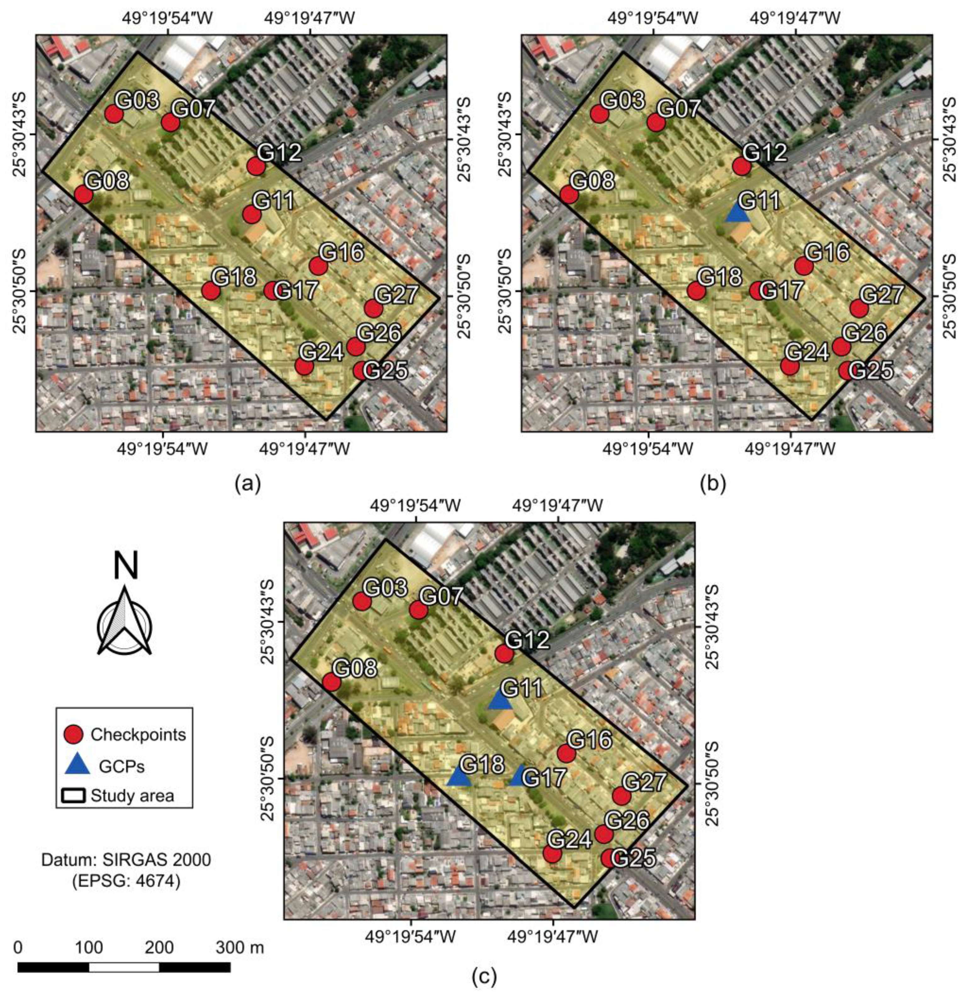
2. Materials and Methods

The photogrammetric survey was conducted in the urban area of Curitiba, Paraná, Brazil, at coordinates 25°30′47″S and 49°19′49″W. The survey covered an area of approximately 12 hectares, characterized as flat terrain. The flight consists of three parallel strips running in the NW-SE direction, totaling 60 aerial images, near to vertical condition, with image forward overlap of 80% and lateral overlap of 70%. The photos of the area were obtained with a flight height of 100 m, resulting in an average ground sample distance (GSD) of 2.84 cm.
For the image acquisition, an Unmanned Aerial System (UAS) Phantom 4 Pro from DJI (Shenzhen, China) was used, with a 1″ CMOS (Complementary Metal Oxide Semiconductor) sensor of 5472 × 3648 pixels, a nominal focal length of 8.8 mm, and pixel size of 2.4 μm. The additional GNSS-PPK receiver module provides the sensor position with a precision of 10 cm in the Xs and Ys camera coordinates and 20 cm in the Zs coordinate, considering the post-processing of GNSS observations performed in the proprietary software of the Guandalini company. In this process, the corrections of the system mounting parameters and time synchronization between camera exposure times and GNSS measurements are also included.
The field survey for determining the geodesic coordinates of reference points (GCPs and checkpoints) was executed by a pair of GNSS Real Time Kinematic (RTK) receivers, Topcon Hiper SR model (Tokyo, Japan), which has a horizontal precision of 10 mm + 0.8 ppm, and a vertical precision of 15 mm + 1.0 ppm [55].
The test version of Agisoft Metashape v 1.5 is used for self-calibration processing using the photogrammetric SfM technique. The measurements of the homologous tie points in the images were carried out autonomously in SfM photogrammetric approach, while the Ground Control Points and checkpoints were measured monoscopically and semi-automatically. For all experiments performed in Metashape, the detail level Highest was set in the process of tie point observations, which yielded a sparse cloud of photogrammetric points.
For GNSS-AAT and on-site calibration procedures with the sub-block of images, the measurements of the tie points are performed autonomously in the Photogrammetry Module of Erdas Imagine. GCPs and checkpoints are measured semi-automatically. In addition, the BBA of GNSS-AAT experiments is also conducted by Erdas Photogrammetric module software.
Federal University of Paraná (UFPR) Calibration Bundle Adjustment Software is used for determining the Interior Orientation Parameters by on-site (in situ) calibration with a sub-block of images.
The coordinate reference system (CRS) utilized for the object space coordinates (X, Y, Z) in all experiments conducted in this study was Datum SIRGAS 2000, and the cartographic projection was UTM zone 22S (EPSG: 31982).
The methodology employed in the present study and the experimental specifications utilized for result comparison are graphically represented in Figure 1.

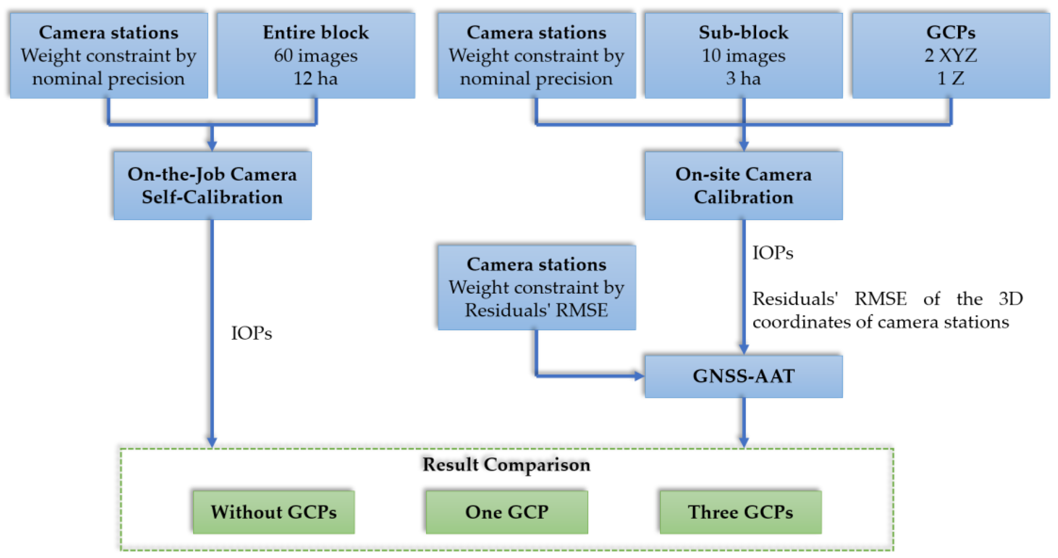
2.1. On-the-Job Camera Self-Calibration

The software Metashape with the SfM approach was used to perform the experiments of on-the-job camera self-calibration. In these experiments, 8.8 mm was used as the initial value for the nominal focal length. All IOPs were calculated in the Metashape self-calibration. In this step, the block with 60 images and three flight strips was used, with the camera station coordinates (Xs, Ys, Zs) measured by the airborne GNSS-PPK receiver.
According to the Metashape user manual [56], the program uses the Conrady-Brown model to obtain the interior orientation of the sensor. Thus, the following parameters were estimated: focal length ( c ), principal point coordinates ( x p , y p ), symmetric radial distortion coefficients ( k 1 , k 2 , k 3 ), and decentering distortion coefficients ( p 1 , p 2 ). For the photogrammetric measurements of the tie points, SfM relies on algorithms that allow the detection, identification, and matching of homologous points, such as SIFT [57]. Subsequently, a Bundle Block Adjustment (BBA) is executed by integrating photogrammetric observations and direct sensor position measurements. The objectives of this BBA are to refine the EOPs, estimate the camera IOPs, and extract 3D object coordinates of the image point feature.
Three self-calibration experiments are proposed in Metashape to evaluate the gain in accuracy derived from the use of Ground Control Points (GCP) in association with the sensor position obtained with GNSS-PPK: without GCP (Figure 2a), with one GCP in the center of the block (Figure 2b) and with three GCP in the central region of the block (Figure 2c). The configuration with three GCPs was established with the same points (G11, G17, and G18) used in the on-site calibration with sub-block. The camera position coordinates (Xs, Ys, Zs) from the GNSS-PPK are included in the bundle adjustment as additional observations by weight constraints, according to the nominal precisions (0.010 m for Xs and Ys coordinates, and 0.020 m for Zs coordinate). Orientation angles (ω, φ, κ) remain unknown to be estimated in the adjustment.
Tridimensional coordinates of 12 reference points were surveyed by geodetic methods using a GNSS-RTK receiver. In each experiment, the points not used as GCPs are defined as checkpoints to verify the accuracy in the extraction of geoinformation obtained with SfM. The GCPs and CPs distributions are shown in Figure 2.

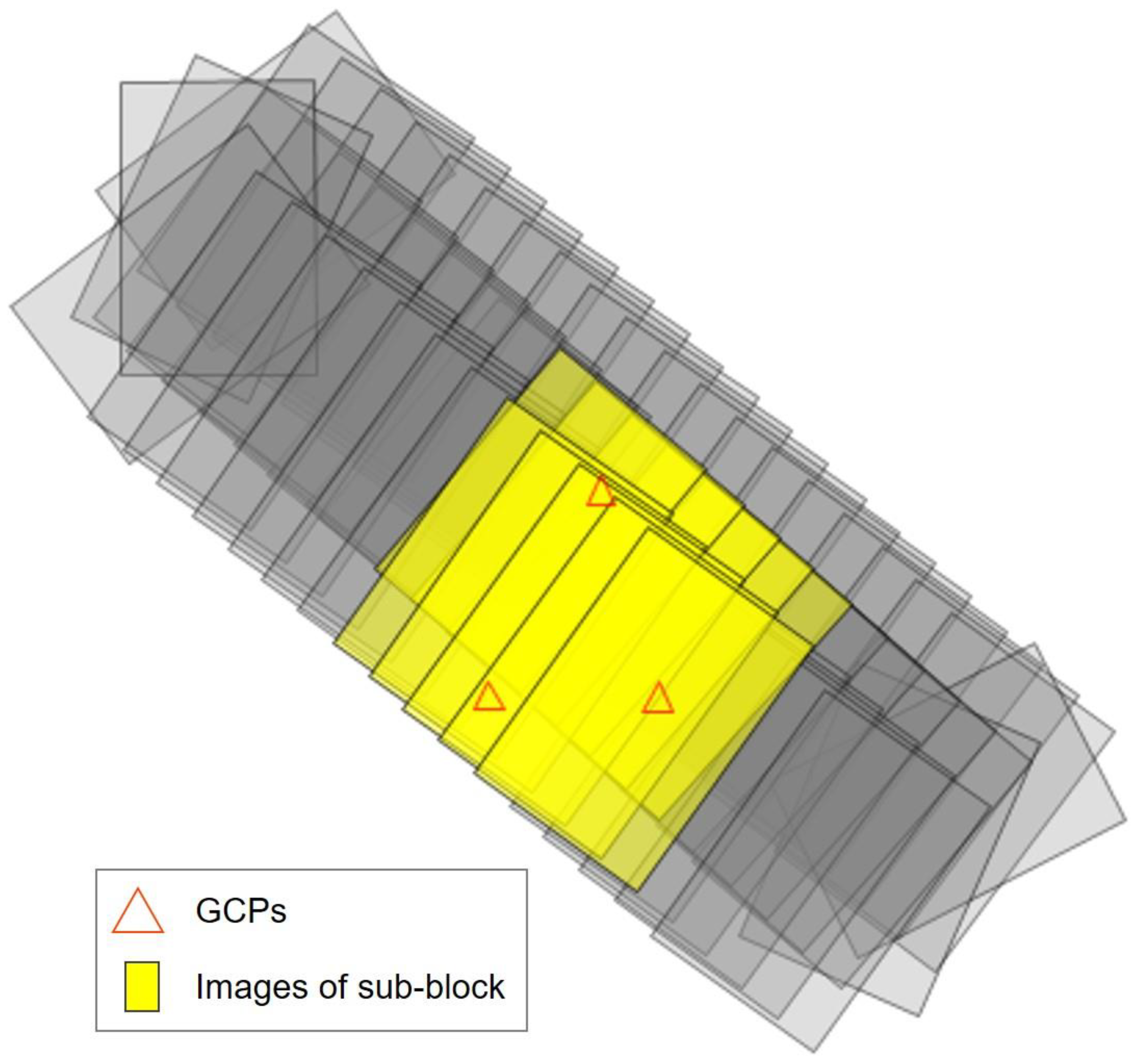
2.2. On-Site Camera Calibration Using Sub-Block of Images

The first step of the on-site calibration is the sub-block definition, i.e., the number of photos and strips that will be used and their location related to the entire block of photos. A set of 10 images, located in the central region of the block, were chosen to compose the sub-block. This configuration was supported by the [54] research regarding on-site calibration with a sub-block of images: among the five sub-block configurations studied in their research (one at each corner of the block and one in the central portion), the sub-block in the central region yielded the best position accuracies in performed experiments of Integrated Sensor Orientation (ISO). Regarding the sub-block dimension, it has two strips flown in opposite directions, with five images in each strip (Figure 3). In addition, the sub-block has only three GCPs, each of which is visible in at least two pictures.
The mathematical model used for camera calibration was proposed by Brown–Conrady [58,59]. In this case, the functional model of the BBA consists of the collinearity equations with IOPs included as additional parameters (Equations (1) and (2)). The tie points were automatically measured near the Von Gruber locations using the Erdas software.
x = c m 11 ( X X s ) + m 12 ( Y Y s ) + m 13 ( Z Z s ) m 31 ( X X s ) + m 32 ( Y Y s ) + m 33 ( Z Z s ) + x p + Δ r a d x + Δ d e c x
y = c m 21 ( X X s ) + m 22 ( Y Y s ) + m 23 ( Z Z s ) m 31 ( X X s ) + m 32 ( Y Y s ) + m 33 ( Z Z s ) + y p + Δ r a d y + Δ d e c y
in which the correction of symmetric radial lens distortion Δ r a d is:
Δ r a d x = ( k 1 r 2 + k 2 r 4 + k 3 r 6 ) ( x x p )
Δ r a d y = ( k 1 r 2 + k 2 r 4 + k 3 r 6 ) ( y y p )
and the correction of decentering lens distortion Δ d e c is:
Δ d e c x = p 1 [ r 2 + 2 ( x x p ) 2 ] + 2 p 2 ( x x p ) ( y y p )
Δ d e c y = 2 p 1 ( x x p ) ( y y p ) + p 2 [ r 2 + 2 ( y y p ) 2 ]
with:
r = ( x x p ) 2 + ( y y p ) 2
where x ,   y are the measured image coordinates of the point; x p , y p are the coordinates of the principal point; c is the focal length; X ,   Y ,   Z are the coordinates of the point in object space; X s ,   Y s ,   Z s are the coordinates of the sensor at the time of exposure; k 1 ,   k 2 ,   k 3 are the symmetric radial distortion coefficients; p 1 ,   p 2 are decentering lens distortions coefficients; and m i , j are the rotation matrix terms for the camera attitude angles.
To perform the on-site calibration, three GCPs were established in the sub-block (two three-dimensional GCPs (G11, G18), and one vertical (G17)), i.e., the minimum configuration to fix the 3D Coordinate System in the object space. Then, an input file required to perform the calibration was generated; this file has the following data: measured coordinates of tie points and GCP points in image space; 3D coordinates of the camera position stations, measured by on-board GNSS-PPK receiver, weighted according to the nominal precisions; approximate values of sensor orientation angles (ω, φ, κ); nominal focal length; pixel size on the sensor of 2.4 μm; the precision of ½ pixel for the imagery observations; Ground Control Points (GCPs) coordinates, in the object-space referential, measured by GNSS-RTK receiver, weighted according to the nominal precisions. From the calibration results, the residuals of image-space coordinates were analyzed to identify possible measurement imprecisions in tie points and GCP points. The maximum tolerance for the residuals was established as three pixels (7.2 μm). Thus, imagery measurements with residuals greater than three pixels were measured again manually or eventually removed from the calibration process.
Furthermore, it is necessary to identify which Interior Orientation Parameters (IOPs) are significant in the camera calibration process or their importance in modeling the displacement of the collinearity condition of an image point and its homologous in the object space. This step can be accomplished by employing hypothesis testing based on the Fisher-Snedecor distribution [60].
For a parameter x i estimated in the adjustment, the following hypotheses are formulated:
  • Null hypothesis ( H 0 ): x i = 0 ;
  • Alternative hypothesis ( H A ): x i 0 ;
For each parameter, the test statistic F x i can be calculated from Equation (8), where σ x i 2 corresponds to the variance of the parameter obtained from the Variance-Covariance Matrix.
F x i = x i 2 σ x i 2
The inverse of the F distribution has two degrees of freedom parameters: the first refers to the number of parameters that will be analyzed and corresponds to the value one since the significance of the IOPs will be checked individually; the second is equivalent to the degree of freedom of the adjustment, i.e., the difference between the number of equations and the number of unknowns. For an arbitrary significance level (α), acceptance of the null hypothesis occurs when the test statistic F x i is less than the inverse of the distribution ( F 1 α , 1 , g l ). Thus, if the null hypothesis is accepted, the parameter analyzed is considered statistically equal to zero and, therefore, is not statistically significant in the mathematical model. If the null hypothesis is rejected, the parameter is evaluated as statistically significant and cannot be eliminated in the model.
The IOPs, not significant statistically on the modeling of the collinearity of the light ray that connects the image point, projection center, and object point, will be weighted as zero. Then, a new calibration will be carried out. Thus, the subsequent GNSS-AAT experiments will use only IOPs statistically significant in the on-site camera calibration process.

2.3. GNSS-AAT Using IOPs from the On-Site Calibration

The obtained results from the GNSS-Assisted Aerial Triangulation, and the on-the-job camera self-calibration, shown in item 2.1, will be compared. To this end, GNSS-AAT (BBA) experiments were carried out in the Erdas Imagine software with the same set and distribution of GCP used in self-calibration experiments performed by Metashape software. In the GNSS-AAT experiments, the IOPs obtained in the on-site camera calibration were fixed. Furthermore, the Root Mean Square Error (RMSE) of the residual camera station coordinates from on-site calibration was used as the uncertainty of camera positions obtained by airborne GNSS-PPK and included in the BBA as additional observations by weight constraint.
Since the camera orientation was not measured directly, the angles estimated in self-calibration without GCP were used as an initial approximation in GNSS-AAT. According to feedback from Agisoft technical support on the company’s official forum [61] and corroborating comparative investigations between the programs performed in this research, the angle of rotation around the Z-axis (κ) is counted counterclockwise in Metashape. Therefore, this angle was converted clockwise to be used as initial parameters in the Erdas program.
The output of Erdas standard report presents the residuals of the photogrammetric measurements at the tie points, which allows more careful analysis of the quality of these measurements in the image space. Based on this report, measurements from tie points with residuals above three pixels (7.2 µm) will be eliminated, ensuring that all measured points remained with observations in at least two images.
It is worth noting that this information can only be accessed in Metashape through the Python API, which restricts its accessibility to individuals familiar with the Python programming language. This limitation may pose a challenge for users who do not possess programming skills. Therefore, it is relevant to develop the possibility of generating a more extensive processing report that includes these and other important information for photogrammetric quality control.
The three GNSS-AAT (BBA) experiments will be executed with the same point distribution of the self-calibrations performed in Metashape software (Figure 2): without Ground Control Points (GCP), with one GCP in the center of the block, and with three GCP in the central area of the block. This configuration of three GCPs in the center of the block was the same configuration and GCPs, used in the sub-block of photos to perform on-site camera calibration (item 2.2). For the three experiments, points not used as GCPs are defined as checkpoints.
For the experiments performed without GCPs or with only one GCP, the 3D coordinate system on the ground cannot be fixed. In these cases, to allow GNSS-AAT (BBA) in the Erdas Software, it was necessary to constrain the position and orientation of the camera station. Since the initial approximation of the orientation angles came from Metashape, the uncertainty of two degrees was established for the orientation angles (ω, φ, κ) so that the weight of these measurements would be significantly low in the adjustment and these parameters could be estimated with high flexibility.

3. Results

3.1. On-the-Job Camera Self-Calibration

The camera self-calibration experiments using a block of 60 images obtained with an Unmanned Aerial System (UAS) were performed by Metashape Software with the SfM approach. Camera position coordinates measured in the on-board GNSS-PPK were constrained in BBA according to the nominal accuracy of the equipment (0.010 m for Xs and Ys coordinates and 0.020 m for Zs coordinates). Table 1 shows the main RMSE results of residuals from self-calibration experiments without GCP, with one GCP, and with three GCP.
Table 1 shows the main results of residuals’ RMSE of the 3D coordinates of camera station positions and 3D coordinates of GCPs used in three Camera Self-Calibration experiments. It can be noted that the values of residuals’ RMSE of the 3D coordinates of camera station positions (Xs, Ys, and Zs) increased with the number of GCPs, included in the self-calibration process. In the experiment without GCPs, the 3D coordinate system on the object space was defined only by the 3D coordinates of the camera station positions. For this condition, the values of residuals’ RMSE of the 3D coordinates of camera station positions are close to the nominal uncertainty of 10 cm. However, using three GCPs, the 3D coordinate system on the object space is defined mainly by the 3D coordinates of the GCPs because their precisions are better than the precisions of 3D coordinates of camera station positions.
In Table 1, the values of residuals’ RMSE of the 3D coordinates of camera station positions and 3D coordinates of the three GCPs are close to the nominal uncertainties of the respective equipment (GNSS-PPK and GNSS-RTK); except for residuals’ RMSE of the Ys coordinates that has a value near to 4x higher than the nominal precision of 10 cm. This outcome suggests that Ys coordinates were computed with higher uncertainty than the value indicated by the manufacturer. Using one GCP in the self-calibration process, the residuals’ RMSE of the 2D coordinates of camera station positions (Xs and Ys) only slightly increased compared to those obtained in the self-calibration process without the use of GCPs. These results are not expected due to the horizontal coordinates of the GCP (X and Y) contributing to the definition of the 2D coordinate system in the object space. On the other hand, the residuals’ RMSE of the vertical coordinates of camera station positions (Zs) is near to 2x higher than the nominal precision of 20 cm, showing that the vertical referential (Z) on the object space was fixed.
The measurements of the homologous points in the images performed autonomously in Metashape software resulted in 78,547 tie points, and the residuals’ RMSE of the photogrammetric measures was equal to 0.4 pixels (0.001 mm) in the self-calibrations experiments without GCP, with one GCP, and with three GCPs.
For all self-calibrations, the interior orientation parameters were estimated by the -Brown-Conrady distortion model: focal length ( c ), principal point coordinates ( x p ,   y p ), radial distortion coefficients ( k 1 ,   k 2 ,   k 3 ), and decentering (tangential) distortion coefficients ( p 1 ,   p 2 ). Table 2 shows the camera calibration parameters estimated in each experiment and their respective standard deviations.
Based on the estimated IOP values, it is possible to notice that the principal point coordinates varied by less than 0.002 mm among the experiments. The radial and decentering distortion coefficients also present minor variations. However, the focal length changes significantly. The difference between the values estimated in the self-calibration without GCP and the experiment with 3 GCP reaches 0.068 mm. This high variation can be explained by the direct mathematical correlation between the focal distance ( c ) and the coordinate (Zs) of the camera station. The Zs coordinate is refined in the BBA and its value variates with the configuration of GCP.
Subsequently, the accuracy of spatial data acquisition by on-the-job camera self-calibration in the Metashape software with the SfM approach can be analyzed by the RMSE of 3D discrepancies from the checkpoints. Table 3 shows the discrepancies in RMSE of the 3D coordinates of the checkpoints and the horizontal (XY) discrepancies in RMSE of the three experiments. The presence of bias in geoinformation extraction was also evaluated. Figure 4a,c,e display a scatter plot with the discrepancies in X and Y for each checkpoint in the experiments without GCP, with one GCP, and with three GCP, respectively. The mean value of discrepancies is highlighted in blue. Similarly, Figure 4b,d,f show the vertical discrepancies (Z) at each checkpoint, with the average value dashed in blue.
Based on obtained results in Table 3, the camera self-calibration without GCPs acquired the lowest positional accuracy; the horizontal and vertical RMSEs are equal to 0.849 m and 0.595 m, respectively. Analyzing the values of obtained discrepancies from the checkpoints in this experiment (Figure 4a,b), it is possible to notice a positive bias in the three coordinates (X, Y, and Z), with the Y coordinate standing out with an average of 0.800 m.
In the camera self-calibration with one GCP, the value of the horizontal RMSE decreased considerably to 0.164 m, and the means discrepancies of X and Y coordinates are close to zero (Figure 4c), fixing the X and Y positive biases that were found in the camera calibration without GCP. On the other hand, the value of the vertical RMSE increased to 0.699 m, and the majority of discrepancies of the Z coordinate remained a positive trend (Figure 4d), with an average value equal to 0.378 m, mainly caused by high positive discrepancies in points G18, G24, and G25.
Outcomes of the camera self-calibration with three GCP (Table 3) show that the horizontal RMSE improved by 71% and the vertical RMSE by 41% compared to the obtained results from the camera self-calibration without GCP. In addition, the vertical discrepancies have a slight negative tendency (Figure 4f), with an average of −0.106 m, thus meaning a reduction in the altimetric bias relative to the other experiments.
Despite the integration of direct measurements of camera station coordinates (Xs, Ys, Zs), the analyses performed in checkpoints discrepancies in this study indicate that the absence of GCP in the camera self-calibration significantly reduces its horizontal and vertical accuracies. The use of one Ground Control Point (GCP) located in the central area of the block during the calibration process resulted in a noteworthy improvement in the horizontal Root Mean Square Error (RMSE). However, no significant improvement was observed in the vertical accuracy. The camera self-calibration with three GCP in the central area of the block (minimum condition to fix the 3D Coordinate System on the ground) provided a significant reduction of the horizontal and vertical bias; in additionally, compared with obtained results from the self-calibration without GCP, the horizontal and vertical accuracies were increased significantly.
The value of the Y discrepancies’ RMSE from the checkpoints analyzed in the self-calibration without GCP, equal to 0.803 m (shown in Table 3 and Figure 4a), shows a probable bias in the Y coordinates of the camera stations. In the same experiment, the residuals’ RMSE of Y coordinates of the camera stations, equal to 0.104 cm (Table 1), is near the nominal precision of the onboard GNSS-PPK (0.10 cm). However, when three GCP were included in the self-calibration experiment, the residuals’ RMSE of Y coordinates changed to 0.468 m. These results reinforce the hypothesis that the Y coordinates of the camera stations may have inaccuracies higher than the nominal uncertainty of the onboard GNSS-PPK. In conclusion, for the dataset used in this study, the on-the-job camera self-calibration without GCP will compromise their horizontal and vertical accuracies.
The self-calibration with three GCP (minimum amount to fix a coordinate system on the object space) achieved more accurate results from the performed experiments; the horizontal and vertical discrepancies’ RMSEs were 0.242 m (8.5 GSD), and 0.308 m (10.8 GSD), respectively. The following topic will entail an investigation of GNSS-AAT using on-site (in situ) camera calibration with a sub-block of images with the aim of enhancing the accuracy of horizontal and vertical measurements in spatial data acquisition.
An additional experiment using on-site calibration was conducted in Metashape Software. This experiment used the same sub-block that is described in Section 3.2. The IOPs were estimated by Metashape Software; the values are, respectively: c = 8.783 mm; x p = −0.007 mm and y p = 0.036 mm; k 1 = 3.21 × 10⁻⁶ mm−2, k 2 = −3.03 × 10⁻⁵ mm−4 and k 3 = 3.18 × 10⁻⁵ mm−6; p 1 = 1.13 × 10⁻⁶ mm−1 and p 2 = −4.49 × 10⁻⁷ mm−1. Afterward, a GNSS-AAT experiment was carried out in Metashape Software. This experiment used the entire block with 3 GCPs (G11, G17, and G18), the IOPs from the on-site camera calibration, and the camera station positions obtained by airborne GNSS-PPK; these values were included in the BBA as additional observations by weight constraint. From this experiment, the horizontal RMSE (XY) of the check-point discrepancies resulted in a value of 0.315 m (11.1 GSD). This value is 30% higher than the value of RMSE XY of 0.242 m (8.5 GSD), obtained from the on-the-job calibration using 3 GCPs performed by Metashape. The vertical RMSE was equal to 0.994 m (35 GSD), three times larger than the RMSE Z of 0.308 m (10.8 GSD) obtained from the on-the-job calibration. The values of IOPs, estimated in on-site calibration with a sub-block, were responsible for these low accuracies. Based on these obtained results, it can be concluded that the Metashape software could not estimate accurate values of IOPs, using a small block. Further investigations will be conducted in future work to understand better this unexpected behavior of the on-site calibration with sub-block in Metashape Software.

3.2. On-Site Camera Calibration

On-site camera calibration was performed to estimate new IOP to improve the quality of geoinformation extraction in the GNSS-AAT approach. To this end, a sub-block was selected in the central area of the block, with ten images and two flight strips running in opposite directions. The sub-block was established in an area that contained three GCPs, all visible in at least two images.
The CALIBRAV program from UFPR was used to perform the on-site calibration. The mathematical model for camera calibration consists of the collinearity equations with additional parameters, which are: focal length ( c ), principal point coordinates ( x p ,   y p ), radial distortion coefficients ( k 1 ,   k 2 ,   k 3 ), and decentering distortion coefficients ( p 1 ,   p 2 ). This on-site calibration procedure was executed with the minimum configuration of points to fix the 3D Coordinate System in the object space, i.e., two three-dimensional GCPs (G11 and G17) and a vertical GCP (G18).
The Erdas Photogrammetric Software was used to perform the photogrammetric measurements. Seventy-six tie points were automatically measured near the “Von Gruber” positions. The nominal focal length, equal to 8.8 mm, and 3D coordinates of the camera positions, measured directly by GNSS-RTK, were included in the Erdas Software to improve the performance of the automatic measurements of the tie points. The GCPs and tie points (not or incorrectly measured) were measured manually. The GCPs and tie points distribution in the sub-block are shown in Figure 5a,b, respectively. In addition, the figures show the image center locations and identifications.
Subsequently, a text file was defined for input in the CALIBRAV program, containing the following information: (1) GCPs coordinates in the geodetic referential measured with GNSS-RTK, (2) camera position coordinates, (3) variance of 3D coordinates of the GCPs and the camera station coordinates, according to the nominal accuracies of the equipment, (4) GCPs and tie points coordinates in the image space, in millimeters, (5) nominal focal length of 8.8 mm, (6) photogrammetric point measurements accuracies of 1/2 pixel, (7) a prior variance of the adjustment equal to 1.0. The GCPs coordinates and the coordinates of the camera stations are included in the calibration process by weight constraints.
Initially, the camera calibration process was performed to estimate the eight Interior Orientation Parameters, defined according to the Brown-Conrady model. A value of three pixels, equal to 7.2 μm, was adopted as the maximum tolerance for residuals in points coordinates in the image space; measurements with residuals above this threshold were remeasured or eliminated. Based on this criterion, only one-point measurement was removed. After this quality control, a new calibration process was carried out, resulting in a posteriori variance equal to 1.07. This value, close to a priori variance, was accepted to conclude the first calibration process.
Afterward, the Fisher-Snedecor test was performed to analyze the statistical significance of the IOPs for the mathematical model. This test attempts to reject or accept the null hypothesis that an estimated parameter is statistically equal to zero. To this end, the test statistic F x i was calculated for each parameter. If the calculated value is less than the inverse of the F distribution (( F 1 α , 1 , g l ), the null hypothesis can be accepted, and the parameter is assumed to be non-significant. In this instance, a new calibration process is performed, fixing (by weight constraint) the value of the non-significant IOP equal to zero. Then, F x i is calculated again for the remaining IOPs. This procedure resulted in five calibrations process. The obtained results are shown in Table 4. The non-significant parameters are fixed to zero and not removed from the mathematical model. Therefore, all calibration processes have the same value of degrees of freedom equal to 470 and, thus, an identical test critical value.
Furthermore, the one-tailed chi-square test was performed on each camera calibration process. This test aims to reject or accept the null hypothesis that a posteriori variance is statistically lower than or equal to the a priori variance (arbitrated as 1.0). Acceptance of the null hypothesis occurs when the calculated chi-square is less than the inverse of the χ 2 distribution ( χ α , g l 2 ). This result, also shown in Table 4, indicates that the parameter constrained by weight as zero does not reflect a considerable increase in the residuals of the adjustment, so it is not statistically significant for the model.
For the Fisher-Snedecor test with a significance level of 10%, the analysis of one parameter in calibration with 470 degrees of freedom has a critical value ( F 0.9 , 1 , 470 ) of 2.72. According to Table 4, in the calibration with eight IOPs (Calib_1), the p 2 , k 1 , k 2 and k 3 parameters presented the calculated F x i value lower than the F 0.9 , 1 , 470 . Then, a new camera calibration (Calib_2) was performed, constraining the p 2 value as zero, and the test statistic was calculated again for the other IOPs. The parameters k 2 and k 3 remained with an F x i value less than the test critical value of 2.72. In the other calibrations (Calib_3 to Calib_5), the parameters were successively constrained as zero, and the calculation of the test statistic was repeated for the remaining IOPs. Overall, the only parameters with test statistic F x i greater than the test critical value were c , x p , y p , k 1 , and p 1 . Based on this test, it can be inferred that   k 2 , k 3 , and p 2 are not statistically significant for the camera calibration.
Afterward, the one-tailed chi-square test was performed. With a significance level of 10% and 470 degrees of freedom, the critical value χ 0.9 , 470 2 is 509.69. According to the results in Table 4, Calib_3 was the only calibration performed whose calculated χ 2 was greater than the test critical value. In this experiment, the value of p 1 was constrained to zero. Consequently, the residuals of Calib_3 increased substantially, and a posteriori variance was found to be statistically higher than a priori variance. In the other calibrations where the values of p 2 , k 1 , k 2 , and k 3 were constrained by weight as zero, the calculated χ 2 values were less than 509.69. Thus, the one-tailed chi-square test indicates that these IOPs ( p 2 ,   k 1 ,   k 2 ,   k 3 ) can be nulled, and the adjustment residuals remain within the expected.
In an overall analysis of the tests performed, the parameters focal length ( c ), principal point coordinates ( x p ,   y p ), radial distortion coefficient k 1 , and decentering distortion coefficient p 1 are statistically significant in at least one of the tests. Therefore, the chosen camera calibration option for further GNSS-AAT experiments is the Calib_5, which has IOPs c , x p , y p , k 1 , and p 1   with non-zero values.
The Calib_5 outcomes show the a posteriori variance equal to 1.075. Furthermore, the values of residuals’ RMSE of the camera station coordinates were 0.129 m for Xs, 0.263 m for Ys, and 0.164 m for Zs; the residuals’ RMSE of the GCPs coordinates were equal to 0.001 m for the X coordinate, 0.003 m for the Y coordinate and 0.004 m for the Z coordinate. In addition, the value of residuals’ RMSE of the image-space measurements was equal to 0.001 mm (0.4 pixels).

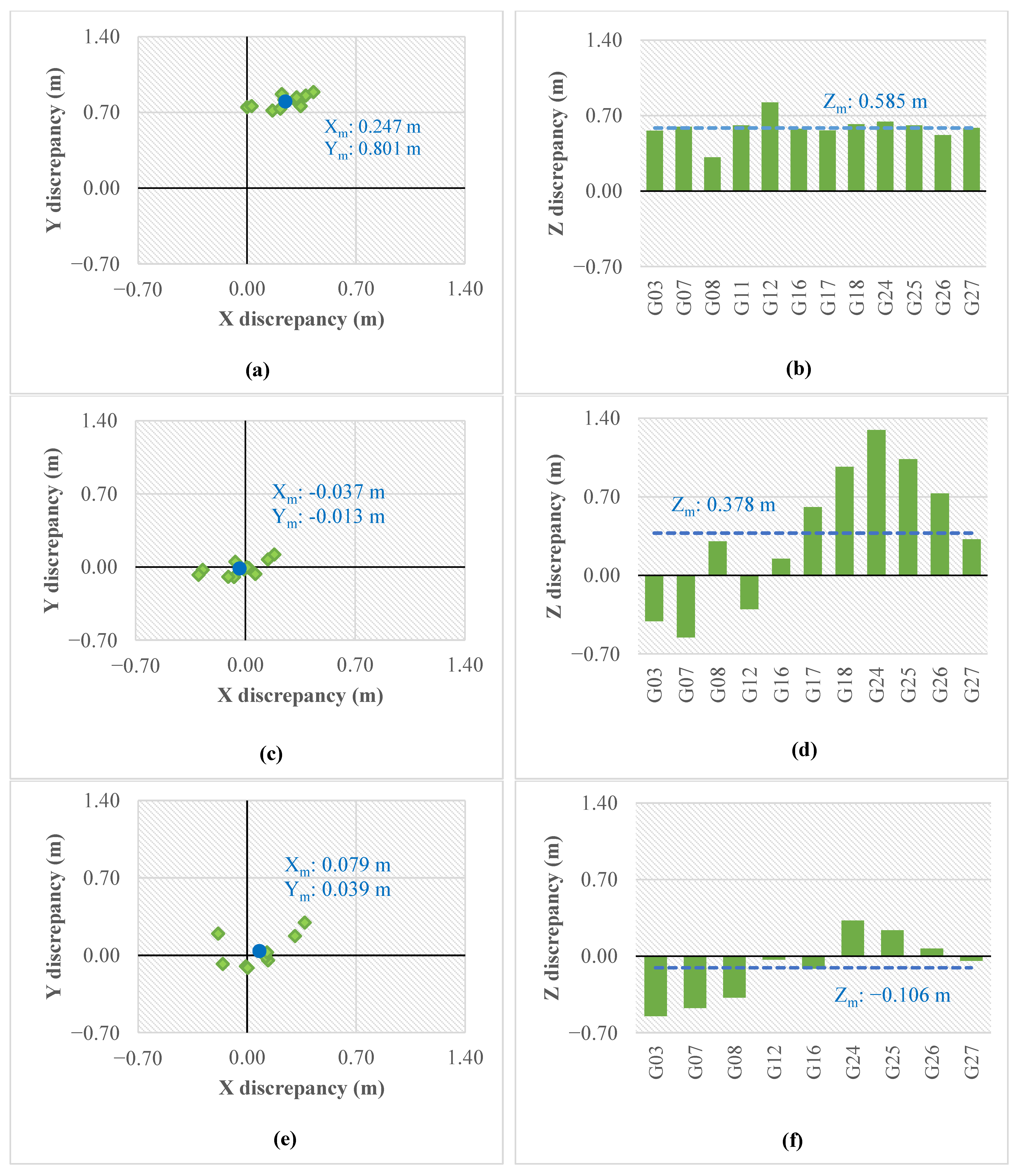
3.3. GNSS-AAT Using IOPs from the On-Site Calibration

The GNSS-Assisted Aerial Triangulation experiments were performed on Erdas Photogrammetric Software, with the same block of 60 images used in the on-the-job self-calibration experiments. To perform these experiments, the IOPs estimated in the on-site calibration with the sub-block of images (Calib_5) were fixed on Erdas software. In GNSS-AAT, the IOPs estimated in the on-site calibration with sub-block of images (Calib_5) were fixed on the BBA (focal length = 9.006 mm, principal point coordinates x p = −0.009 mm and y p = −0.002 mm, radial distortion coefficient k 1 = 9.274 × 10⁻⁶ mm−2, and decentering distortion coefficient p 1 = 6.121 × 10⁻⁵ mm−1).
Furthermore, the camera station coordinates obtained by GNSS-PPK were included in the BBA using weighted constraint, according to the precisions estimated in on-site calibration: 0.129 m for Xs, 0.263 m for Ys, and 0.164 m for Zs. According to the proposal shown by [53], these precisions are more suitable than the nominal values of the GNSS-PPK. Table 5 shows the main residuals’ RMSE results from GNSS-AAT experiments without GCP, with one GCP, and with 3 GCP in the central region of the block.
Analyzing the residuals’ RMSE in Table 5, the residuals’ RMSE of Xs coordinates have minor variation among the experiments, with values slightly higher than the nominal uncertainty of GNSS-PPK measurements (10 cm). On the other hand, the values of residuals’ RMSE of the Ys coordinates increased significantly with the number of GCPs added in the process, reaching 0.579 m in the experiment with 3 GCP; the values of residuals’ RMSE of the Zs coordinates are less than the GNSS-PPK measurements (20 cm). For the results from the GCPs analysis, the values of residuals’ RMSE of 3D coordinates were near the precisions of GNSS-RTK considered in this study. In conclusion, the majority of obtained results from the three GNSS-AAT experiments are similar to those obtained in the on-the-job camera self-calibration experiments, shown and discussed previously in Section 3.1. However, the obtained results using one GCP have a significant difference in the processes. As expected, the residuals’ RMSE of the 2D coordinates of camera station positions (Xs and Ys) increased in the GNSS-ATT.
In general, the values of the residuals’ RMSE of the 3D coordinates of camera station positions and GCPs maintain according to the nominal precisions of the respective GNSS receivers used in this study. However, in the two experiments using GCPs, the values of RMSEs of the Ys camera station coordinates are significantly higher than the nominal precisions (10 cm) provided by the airborne GNSS-PPK manufacturer. These results corroborate the conclusion drawn in the on-the-job-self-calibration experiments that there may be a bias in the Ys coordinates of camera station positions.
Furthermore, the automatic measurement of tie points in the Erdas software near the Von Gruber locations resulted in 818 tie points, and the residuals’ RMSE of the image-space measures was equal to 0.4 pixels (0.001 mm) in all three GNSS-AAT experiments.
The values of discrepancies’ RMSE from 3D coordinates of checkpoints for each experiment were computed to evaluate the accuracies of the GNSS-AAT procedure for spatial data acquisition. Table 6 shows the values of discrepancies’ RMSE of the X, Y, and Z coordinates of checkpoints and the value of horizontal discrepancies’ RMSE. In addition, the occurrence of systematic errors in the three-dimensional coordinates obtained by the GNSS-AAT procedure is investigated. For this purpose, Figure 6a,c,e show the discrepancies of X and Y coordinates of the checkpoints in the GNSS-AAT experiments without GCP, with one GCP, and with three GCP; additionally, the mean value of the discrepancies is highlighted in blue. The discrepancies of Z coordinates (vertical) are represented analogously in Figure 6b,d,f, highlighting the mean value on the dashed blue line.
Table 6 shows the discrepancies in RMSE of 3D coordinates of the checkpoints from the performed GNSS-AAT experiments. The vertical RMSE from the GNSS-AAT without the GCP experiment indicates a significant vertical accuracy that can be confirmed from values of vertical discrepancies of the checkpoints shown in Figure 6b. This vertical accuracy differs from that obtained in the on-the-job camera calibration experiment. This better accuracy is connected to the new value of focal distance, estimated previously in on-site calibration. On the other hand, the horizontal accuracy, shown in Table 6, is close to that obtained in the on-the-job camera calibration experiment. The new values of the principal point coordinates ( x p and y p ), previously estimated in on-site calibration, could not fix the X and Y bias. Therefore, it is possible to notice a positive bias in the X and Y coordinates of the checkpoints (Figure 6a), especially in the Y coordinate with the mean discrepancies close to 0.8 m.
The obtained horizontal accuracy from the GNSS-AAT with one GCP experiment, shown in Table 6 and Figure 6c, significantly improved from the accuracy reached in the experiment of the GNSS-AAT without GCP. This result was not expected, considering that only one GCP does not have geometric properties to fix the 3D coordinate system on the ground, minimizing the Y bias found in the GNSS-AAT without the GCP experiment.
Another unexpected result in this experiment is the vertical accuracy, shown in Table 6 and Figure 6d; its value is lower than that obtained in the investigation of the GNSS-AAT without GCP. The first thought was that the Z coordinate of the GCP has outliers, but the obtained results from the experiment of the GNSS-AAT with three GCPs did not show this problem. Future studies will be performed to find an answer to these unexpected results. In the experiment of the GNSS-AAT with three GCPs, the horizontal and vertical RMSE values of checkpoints’ discrepancies, shown in Table 6, are equal to 0.222 m and 0.154 m, respectively. The obtained horizontal and vertical accuracies in this experiment, shown in Figure 6e,f, reached acceptable accuracies near the precisions of the positions of the camera station adopted in this study (direct measured by the GNSS-PPK). Additionally, the value of the average discrepancy of the Y coordinate of the checkpoints, shown in Figure 6e, was close to zero, indicating the Y bias, found in the GNSS-AAT without GCP, was fixed on the object space in this experiment.
Overall, the performed GNSS-AAT experiments using IOPs from on-site calibration showed different results between their horizontal and vertical accuracy. Only the investigation of the GNSS-AAT with three GCPs yielded horizontal and vertical accuracies close to nominal precisions of the camera station positions by GNSS-PPK measurements adopted in this study. These accuracies were considered by the values of discrepancies’ RMSE of the X, Y, and Z coordinates of checkpoints, equal to 0.157 m, 0.157 m, and 0.154 m, respectively; additionally, the average discrepancies, close to zero, in the three coordinates axis, show an insignificant bias on the 3D coordinates of the object space.

4. Discussion

4.1. Influence of On-Site Camera Calibration with Sub-Block of Images

In accordance with the findings of [25], for Unmanned Aerial System (UAS) Photogrammetry with direct measurements of camera station coordinates by GNSS receiver (RTK or PPK), the bias in the vertical coordinate during the on-the-job self-calibration experiment without Ground Control Points (GCPs) is directly associated with the incorrect estimation of Interior Orientation Parameters (IOPs), particularly the focal distance. To enhance the accuracy of IOPs’ estimation, the inclusion of oblique images [23] or nadir images of multiple flight heights [51] are potential strategies related to the block geometry. These strategies have the potential to reduce the high correlation between focal length ( c ) and the vertical coordinate of the camera station (Zs) and thus improve vertical accuracy.
In general, the utilization of strips at the same height, even if the flight strips are perpendicular (cross-strips), only affects the determination of the principal point coordinates and has not demonstrated a significant improvement in three-dimensional (3D) measurement accuracy in similar studies [25,62]. However, it may not always be feasible to obtain vertical images of multiple flight heights or oblique images. Another approach to mitigate the correlations between the parameters estimated in the Bundle Block Adjustment (BBA) and enhance the accuracy of the UAS survey is to conduct an on-site (in situ) camera pre-calibration [41].
Therefore, the objective of this study was to examine the impact of on-site camera calibration with a sub-block of images on the precision of spatial data acquired through PPK-based UAS photogrammetry. To achieve this, the obtained results from the on-the-job camera self-calibration experiments in Metashape software are compared to those obtained from the GNSS-AAT experiments with on-site calibration using Erdas Imagine software. Without GCP, the horizontal accuracy remained equivalent in both experiments, with a difference of only 1%. On the other hand, the investigation of the GNSS-AAT yielded an 83% improvement in vertical accuracy, or there was a reduction in RMSE Z from 0.595 m (20.9 GSD) to 0.103 m (3.6 GSD). By adding one GCP in the center of the block, horizontal accuracy remains similar in the Metashape and Erdas experiments, with a 10% improvement in the Metashape software. However, in the vertical accuracy, the GNSS-AAT experiment achieved a 47% improvement, or there was a reduction in RMSE Z from 0.699 m (24.6 GSD) to 0.373 m (13.1 GSD).
It is worth noting that there was a significant improvement in the vertical accuracy in the GNSS-AAT experiments without GCPs and with one GCP. Nevertheless, it occurs mainly because the on-site calibration required two three-dimensional GCPs and one vertical GCP in the sub-block of images, and the GNSS-AAT experiments used IOPs from this calibration. In contrast, similar on-the-job camera self-calibration experiments in Metashape Software have none or only one GCP.
In contrast to the experiments of the GNSS-ATT without and with one GCP, analyzed previously, the investigation of the GNSS-ATT with three GCP uses the G11, G17, and G18 (shown in Figure 2c) and IOPs from the on-site calibration performed with the same three GCPs, but in one of them, only the Z coordinate was considered. In this case, the on-site camera calibration on the sub-block of images, shown and discussed previously in item 3.2, improved the accuracy of spatial data acquisition compared to the on-the-job camera self-calibration process performed in this study. Standing out that the values of residuals’ RMSE of the camera station coordinates, estimated in this calibration process and used as new precisions in the GNSS-AAT, contributed too to this improvement.
Thus, the horizontal accuracies (RMSEs XY values) of on-the-job camera self-calibration and GNSS-AAT maintained similar results, but in the GNSS-AAT, there was an 8% improvement. On the other hand, the vertical accuracy (RMSE Z) of 0.308 m (10.8 GSD) in on-the-job camera self-calibration reduces to 0.154 m (5.4 GSD) in GNSS-AAT, reflecting the 50% improvement in vertical accuracy.
In comparison to other pre-calibration methods with a test field, the adoption of a sub-block of images obviates the need for supplementary photogrammetric surveys. Thus, the fieldwork remains essentially the same as that used for spatial data acquisition, similar to the self-calibration approach. In the GNSS-AAT method utilizing on-site calibration with a sub-block of images, the computation time is also comparable to the self-calibration, given that pre-calibration occurs with a subset of the aerial survey. However, it is crucial to note that the analytical processes for assessing the significance of the parameters of the on-site calibration conducted in this article require more circumspect data treatment and an additional working time, as repeated calibration attempts may be necessary to determine the statistically significant IOPs required for modeling lens distortions.

4.2. Influence of GCP Configuration

For UAS photogrammetric surveys integrating camera station coordinates obtained with an on-board GNSS receiver, in the absence of GCPs, the accuracy of spatial data acquisition is highly dependent on the precision of camera position measurement, even with improved flight configurations [20]. This study confirmed the aforementioned dependency through on-the-job self-calibration and GNSS-AAT experiments conducted without GCPs. The mean discrepancies in the Y coordinate of the checkpoints were approximately 80 cm in both experiments without GCP, potentially resulting from a bias in the Y coordinate of the camera station. The existence of such a bias appears to be confirmed when GCPs were included in the experiments, where the residuals of the Ys camera station coordinates notably increased, yielding a residuals’ RMSE of 0.468 m in the on-the-job self-calibration with three GCPs and 0.579 m in the GNSS-AAT with three GCPs. These values were five times higher than the assumed nominal precision of 0.010 m.
On the other hand, the addition of a single GCP revealed a significant improvement in the tendencies of horizontal discrepancies in both the on-the-job self-calibration and GNSS-AAT experiments, resulting in average discrepancies of the checkpoints close to zero for the X and Y coordinates. However, the tendency in the Z discrepancies remained high, with an average of 0.378 m in the on-the-job calibration experiment with one GCP and 0.186 m in the GNSS-AAT experiment with one GCP.
In agreement with the findings of [16,30], the addition of up to three GCPs reveals a noteworthy reduction in vertical errors. However, the on-the-job calibration experiment with 3 GCPs still presents a negative trend of −0.106 m in the discrepancies of the checkpoints. The remaining bias directly affects the vertical accuracy of this experiment, with an RMSE Z value of 0.308 m (10.8 GSD). This result can be explained by the position of the GCPs used in the experiments in this study, which are not well-distributed geometrically in the block as suggested by [15,20]. This is because the established GCPs are concentrated in the central region of the block, with the same points (G11, G17, and G18) used in the on-site calibration with sub-block.
On the other hand, for the GNSS-AAT with 3 GCPs experiment using on-site pre-calibration with sub-block, the average discrepancies of the Z coordinate of the checkpoints showed a value of 0.020 m, reflecting a 50% improvement in vertical accuracy, with the RMSE Z of 0.154 m (5.4 GSD).
In photogrammetric applications with UAS, it may be necessary to concentrate GCPs in a specific region due to the limited accessibility of the area for field surveys [41]. Based on the results of this study, in such cases, the photogrammetric procedure of the GNSS-AAT with on-site camera calibration using sub-block of images can serve as a viable alternative to improve the vertical accuracies in the extraction of spatial information using a UAV platform equipped with the GNSS-PPK receivers.
Even with the inclusion of a minimum GCP configuration in data acquisition, this step requires fieldwork to obtain the three-dimensional coordinates of GCP, which can increase the cost and execution time of the survey, particularly in areas that are difficult to access, such as those that have experienced natural disasters, areas with dense vegetation, or rural areas lacking transportation and mobility infrastructure. From a practical standpoint, the inclusion of a minimum number of GCPs can increase a few days of fieldwork, depending on the chosen survey method and location accessibility. However, the possibility of concentrating GCPs in a small area of the block mitigates these factors by facilitating survey logistics, minimizing the need to relocate professionals and equipment, and enabling the materialization of points in a more accessible region. In urban areas, conducting geodetic/topographic surveys of a few GCPs can be faster and more cost-effective due to the ease of transportation.

5. Conclusions

This research aimed to evaluate the influence of on-site camera calibration on photogrammetric procedures for georeferencing data acquisition integrated with the direct measurement of the camera positions in the UAS platform equipped with a GNSS-PPK receiver. For this purpose, a block of 60 photos was used to perform studies of on-the-job camera self-calibration in the Metashape software with SfM approach and the GNSS-Assisted Aerial Triangulation with on-site calibration in the Erdas Imagine software. For the on-site calibration, a sub-block of 10 images was chosen in the central area of the block, with 3GCPs visible in at least two images.
The on-the-job-camera self-calibration experiments were performed with three configurations: without GCPs, with one GCP in the central area of the block, and with three GCPs in the central area of the block. The results from these three experiments show a significant variation in the focal length values. The maximum difference is close to 0.068 mm. This instability of the focal length can be explained by the readjustment of Zs coordinate with GCP configuration because there is a direct mathematical correlation between these parameters in BBA. The analysis of the discrepancies in checkpoints shows high values of horizontal RMSE and vertical RMSE in the experiment without GCPs. Adding one GCP on the central area of the block the horizontal RMSE improves significantly. However, the vertical RMSE remained higher than the nominal uncertainty of the onboard GNSS-PPK. Only in the experiment with three GCPs the vertical accuracy was improved, achieving more accurate results from the three performed experiments; the horizontal and vertical discrepancies’ RMSEs were 0.242 m (8.5 GSD) and 0.308 m (10.8 GSD), respectively
The experiments of the GNSS-ATT without, with one GCP, and with three GCP increased the accuracy of spatial data acquisition compared to the on-the-job camera self-calibration process. In the GNSS-ATT without GCP, the horizontal accuracy remained equivalent in both experiments, with a difference of only 1%. On the other hand, the investigation of the GNSS-AAT yielded an 83% improvement in vertical accuracy, or there was a reduction in RMSE Z from 0.595 m (20.9 GSD) to 0.103 m (3.6 GSD). Adding one GCP in the center of the block, horizontal accuracy remains similar in both experiments, with a 10% improvement in the on-the-job camera self-calibration. However, in the vertical accuracy, the GNSS-AAT experiment achieved a 47% improvement, or there was a reduction in RMSE Z from 0.699 m (24.6 GSD) to 0.373 m (13.1 GSD). In the experiments with three GCP, the horizontal accuracies (RMSE XY) maintained similar results, but in the GNSS-AAT, there was an 8% improvement. Additionally, the vertical accuracy (RMSE Z) of 0.308 m (10.8 GSD) in on-the-job camera self-calibration reduced to 0.154 m (5.4 GSD) in GNSS-AAT, reflecting the 50% improvement in vertical accuracy.
From the obtained results acquired from the performed experiments using the datasets tested in this study, it can be concluded that the use of on-site camera calibration with a sub-block of images is an important approach to improve the vertical accuracies of the geoinformation dataset, extracted in photogrammetric procedures with the integration of direct measurements of camera station positions using UAS equipped with GNSS-PPK receiver.

Limitations and Future Work

The primary aim of this paper is to emphasize the influence of on-site camera calibration in PPK-based UAS Photogrammetry, utilizing a small sub-block of images with a minimal configuration of control points. However, it should be noted that this study has the limitation of utilizing only a sparse distribution of tie points near “Von Gruber” regions. Such tie-point distributions are typically employed for modeling the distortion of professional photogrammetric cameras equipped with high-quality optical sensors. The utilization of the IOP estimated from on-site calibration as fixed parameters in the experiments conducted in Erdas software yielded promising results by improving the 3D accuracy of spatial data acquisition, even when considering that the cameras onboard UAS commonly utilize low-cost and lower-quality optical cameras.
However, in preliminary experiments conducted in this study, the utilization of IOPs obtained through on-site calibration with a sub-block of images in Metashape resulted in a substantial disparity in the estimated focal length compared to the other calibration methods employed in this study. This discrepancy significantly compromised the vertical accuracy of data acquisition. Therefore, future research may conduct a more meticulous analysis with additional investigations to better understand the possible causes of this unexpected behavior of the on-site calibration with sub-block in Metashape.
Another limitation of this study is the investigation of a single study area and the use of a flight configuration with nadir images at the same altitude. To increase the robustness and generalizability of the findings in future work, it is recommended to include additional flight cases (e.g., oblique images or nadir images acquired at various flight altitudes), use various instrumentation (e.g., diverse cameras and UAV platforms) and explore applications in areas with different terrain type (e.g., coastal regions with varying elevations and mountainous regions with steep slopes).
Regarding the use of direct measurements of sensor position, biases in the 3D coordinates of the camera stations can significantly reduce the accuracy of the spatial data acquisition, especially when a set of GCPs is not used. Future work can investigate the influence of outliers and biases in the camera position measurements on the IOP estimation and the accuracy of spatial information extraction with UAS imagery.

Author Contributions

Conceptualization, K.P. and E.M.; methodology, K.P. and E.M.; validation E.M.; formal analysis, K.P.; investigation, K.P.; resources, E.M.; data curation, K.P.; writing—original draft preparation, K.P.; writing—review and editing, K.P. and E.M; visualization, K.P.; supervision, E.M.; project administration, K.P.; funding acquisition, E.M. All authors have read and agreed to the published version of the manuscript.

Funding

This research was funded by CNPq (National Council for Scientific and Technological Development), grant number 141397/2021-7.

Data Availability Statement

Not applicable.

Acknowledgments

The authors would like to thank Marlo Martins for providing the dataset utilized in this research.

Conflicts of Interest

The authors declare no conflict of interest.

References

  1. Granshaw, S.I. RPV, UAV, UAS, RPAS … or Just Drone? Photogramm. Rec. 2018, 33, 160–170. [Google Scholar] [CrossRef]
  2. Tuffen, H.; James, M.R.; Castro, J.M.; Schipper, C.I. Exceptional Mobility of an Advancing Rhyolitic Obsidian Flow at Cordón Caulle Volcano in Chile. Nat. Commun. 2013, 4, 2709. [Google Scholar] [CrossRef] [Green Version]
  3. Civico, R.; Ricci, T.; Scarlato, P.; Andronico, D.; Cantarero, M.; Carr, B.B.; De Beni, E.; Del Bello, E.; Johnson, J.B.; Kueppers, U.; et al. Unoccupied Aircraft Systems (UASs) Reveal the Morphological Changes at Stromboli Volcano (Italy) before, between, and after the 3 July and 28 August 2019 Paroxysmal Eruptions. Remote Sens. 2021, 13, 2870. [Google Scholar] [CrossRef]
  4. Castillo, C.; Pérez, R.; James, M.R.; Quinton, J.N.; Taguas, E.V.; Gómez, J.A. Comparing the Accuracy of Several Field Methods for Measuring Gully Erosion. Soil Sci. Soc. Am. J. 2012, 76, 1319–1332. [Google Scholar] [CrossRef] [Green Version]
  5. Eltner, A.; Baumgart, P.; Maas, H.-G.; Faust, D. Multi-Temporal UAV Data for Automatic Measurement of Rill and Interrill Erosion on Loess Soil: Uav Data for Automatic Measurement Of Rill And Interrill Erosion. Earth Surf. Process. Landf. 2015, 40, 741–755. [Google Scholar] [CrossRef]
  6. James, M.R.; Robson, S.; Smith, M.W. 3-D Uncertainty-Based Topographic Change Detection with Structure-from-Motion Photogrammetry: Precision Maps for Ground Control and Directly Georeferenced Surveys: 3-D Uncertainty-Based Change Detection for SfM Surveys. Earth Surf. Process. Landf. 2017, 42, 1769–1788. [Google Scholar] [CrossRef]
  7. Niethammer, U.; James, M.R.; Rothmund, S.; Travelletti, J.; Joswig, M. UAV-Based Remote Sensing of the Super-Sauze Landslide: Evaluation and Results. Eng. Geol. 2012, 128, 2–11. [Google Scholar] [CrossRef]
  8. Lucieer, A.; de Jong, S.M.; Turner, D. Mapping Landslide Displacements Using Structure from Motion (SfM) and Image Correlation of Multi-Temporal UAV Photography. Prog. Phys. Geogr. Earth Environ. 2014, 38, 97–116. [Google Scholar] [CrossRef]
  9. Cho, J.; Lee, J.; Lee, B. Application of UAV Photogrammetry to Slope-Displacement Measurement. KSCE J. Civ. Eng. 2022, 26, 1904–1913. [Google Scholar] [CrossRef]
  10. Bemis, S.P.; Micklethwaite, S.; Turner, D.; James, M.R.; Akciz, S.; Thiele, S.T.; Bangash, H.A. Ground-Based and UAV-Based Photogrammetry: A Multi-Scale, High-Resolution Mapping Tool for Structural Geology and Paleoseismology. J. Struct. Geol. 2014, 69, 163–178. [Google Scholar] [CrossRef]
  11. Vasuki, Y.; Holden, E.-J.; Kovesi, P.; Micklethwaite, S. Semi-Automatic Mapping of Geological Structures Using UAV-Based Photogrammetric Data: An Image Analysis Approach. Comput. Geosci. 2014, 69, 22–32. [Google Scholar] [CrossRef]
  12. Ryan, J.C.; Hubbard, A.L.; Box, J.E.; Todd, J.; Christoffersen, P.; Carr, J.R.; Holt, T.O.; Snooke, N. UAV Photogrammetry and Structure from Motion to Assess Calving Dynamics at Store Glacier, a Large Outlet Draining the Greenland Ice Sheet. Cryosphere 2015, 9, 1–11. [Google Scholar] [CrossRef] [Green Version]
  13. Belloni, V.; Fugazza, D.; Di Rita, M. Uav-Based Glacier Monitoring: Gnss Kinematic Track Post-Processing and Direct Georeferencing for Accurate Reconstructions in Challenging Environments. Int. Arch. Photogramm. Remote Sens. Spatial Inf. Sci. 2022, XLIII-B1-2022, 367–373. [Google Scholar] [CrossRef]
  14. Deliry, S.I.; Avdan, U. Accuracy of Unmanned Aerial Systems Photogrammetry and Structure from Motion in Surveying and Mapping: A Review. J. Indian Soc. Remote Sens. 2021, 49, 1997–2017. [Google Scholar] [CrossRef]
  15. Liu, Y.; Han, K.; Rasdorf, W. Assessment and Prediction of Impact of Flight Configuration Factors on UAS-Based Photogrammetric Survey Accuracy. Remote Sens. 2022, 14, 4119. [Google Scholar] [CrossRef]
  16. Pargieła, K.; Rzonca, A. Determining Optimal Photogrammetric Adjustment of Images Obtained from a Fixed-wing UAV. Photogramm. Rec. 2021, 36, 285–302. [Google Scholar] [CrossRef]
  17. Sanz-Ablanedo, E.; Chandler, J.; Rodríguez-Pérez, J.; Ordóñez, C. Accuracy of Unmanned Aerial Vehicle (UAV) and SfM Photogrammetry Survey as a Function of the Number and Location of Ground Control Points Used. Remote Sens. 2018, 10, 1606. [Google Scholar] [CrossRef] [Green Version]
  18. Ferrer-González, E.; Agüera-Vega, F.; Carvajal-Ramírez, F.; Martínez-Carricondo, P. UAV Photogrammetry Accuracy Assessment for Corridor Mapping Based on the Number and Distribution of Ground Control Points. Remote Sens. 2020, 12, 2447. [Google Scholar] [CrossRef]
  19. Gomes Pessoa, G.; Caceres Carrilho, A.; Takahashi Miyoshi, G.; Amorim, A.; Galo, M. Assessment of UAV-Based Digital Surface Model and the Effects of Quantity and Distribution of Ground Control Points. Int. J. Remote Sens. 2021, 42, 65–83. [Google Scholar] [CrossRef]
  20. Liu, X.; Lian, X.; Yang, W.; Wang, F.; Han, Y.; Zhang, Y. Accuracy Assessment of a UAV Direct Georeferencing Method and Impact of the Configuration of Ground Control Points. Drones 2022, 6, 30. [Google Scholar] [CrossRef]
  21. Gerke, M.; Nex, F.; Remondino, F.; Jacobsen, K.; Kremer, J.; Karel, W.; Hu, H.; Ostrowski, W. Orientation of Oblique Airborne Image Sets &Ndash; Experiences from the Isprs/Eurosdr Benchmark on Multi-Platform Photogrammetry. Int. Arch. Photogramm. Remote Sens. Spatial Inf. Sci. 2016, XLI-B1, 185–191. [Google Scholar] [CrossRef] [Green Version]
  22. James, M.R.; Robson, S. Mitigating Systematic Error in Topographic Models Derived from UAV and Ground-Based Image Networks: Mitigating Systematic Error in Topographic Models. Earth Surf. Process. Landf. 2014, 39, 1413–1420. [Google Scholar] [CrossRef] [Green Version]
  23. Carbonneau, P.E.; Dietrich, J.T. Cost-Effective Non-Metric Photogrammetry from Consumer-Grade SUAS: Implications for Direct Georeferencing of Structure from Motion Photogrammetry: Cost-Effective Non-Metric Photogrammetry from Consumer-Grade SUAS. Earth Surf. Process. Landf. 2017, 42, 473–486. [Google Scholar] [CrossRef] [Green Version]
  24. Gerke, M.; Przybilla, H.-J. Accuracy Analysis of Photogrammetric UAV Image Blocks: Influence of Onboard RTK-GNSS and Cross Flight Patterns. Photogramm. Fernerkund. Geoinf. 2016, 2016, 17–30. [Google Scholar] [CrossRef] [Green Version]
  25. Štroner, M.; Urban, R.; Seidl, J.; Reindl, T.; Brouček, J. Photogrammetry Using UAV-Mounted GNSS RTK: Georeferencing Strategies without GCPs. Remote Sens. 2021, 13, 1336. [Google Scholar] [CrossRef]
  26. Stumpf, A.; Malet, J.-P.; Allemand, P.; Pierrot-Deseilligny, M.; Skupinski, G. Ground-Based Multi-View Photogrammetry for the Monitoring of Landslide Deformation and Erosion. Geomorphology 2015, 231, 130–145. [Google Scholar] [CrossRef]
  27. Kameyama, S.; Sugiura, K. Effects of Differences in Structure from Motion Software on Image Processing of Unmanned Aerial Vehicle Photography and Estimation of Crown Area and Tree Height in Forests. Remote Sens. 2021, 13, 626. [Google Scholar] [CrossRef]
  28. Jiang, S.; Jiang, C.; Jiang, W. Efficient Structure from Motion for Large-Scale UAV Images: A Review and a Comparison of SfM Tools. ISPRS J. Photogramm. Remote Sens. 2020, 167, 230–251. [Google Scholar] [CrossRef]
  29. Gonçalves, J.A.; Henriques, R. UAV Photogrammetry for Topographic Monitoring of Coastal Areas. ISPRS J. Photogramm. Remote Sens. 2015, 104, 101–111. [Google Scholar] [CrossRef]
  30. Grayson, B.; Penna, N.T.; Mills, J.P.; Grant, D.S. GPS Precise Point Positioning for UAV Photogrammetry. Photogramm. Rec. 2018, 33, 427–447. [Google Scholar] [CrossRef] [Green Version]
  31. Vericat, D.; Brasington, J.; Wheaton, J.; Cowie, M. Accuracy Assessment of Aerial Photographs Acquired Using Lighter-than-Air Blimps: Low-Cost Tools for Mapping River Corridors. River Res. Applic. 2009, 25, 985–1000. [Google Scholar] [CrossRef]
  32. Turner, D.; Lucieer, A.; Watson, C. An Automated Technique for Generating Georectified Mosaics from Ultra-High Resolution Unmanned Aerial Vehicle (UAV) Imagery, Based on Structure from Motion (SfM) Point Clouds. Remote Sens. 2012, 4, 1392–1410. [Google Scholar] [CrossRef] [Green Version]
  33. Chiabrando, F.; Giulio Tonolo, F.; Lingua, A. UAV Direct Georeferencing Approach in An Emergency Mapping Context. The 2016 Central Italy Earthquake Case Study. Int. Arch. Photogramm. Remote Sens. Spatial Inf. Sci. 2019, XLII-2/W13, 247–253. [Google Scholar] [CrossRef] [Green Version]
  34. Antoine, R.; Lopez, T.; Tanguy, M.; Lissak, C.; Gailler, L.; Labazuy, P.; Fauchard, C. Geoscientists in the Sky: Unmanned Aerial Vehicles Responding to Geohazards. Surv. Geophys. 2020, 41, 1285–1321. [Google Scholar] [CrossRef]
  35. Benjamin, A.R.; O’Brien, D.; Barnes, G.; Wilkinson, B.E.; Volkmann, W. Improving Data Acquisition Efficiency: Systematic Accuracy Evaluation of GNSS-Assisted Aerial Triangulation in UAS Operations. J. Surv. Eng. 2020, 146, 05019006. [Google Scholar] [CrossRef]
  36. Yastikli, N.; Jacobsen, K. Influence of System Calibration on Direct Sensor Orientation. Photogramm. Eng. Remote Sens. 2005, 71, 629–633. [Google Scholar] [CrossRef] [Green Version]
  37. Turner, D.; Lucieer, A.; Wallace, L. Direct Georeferencing of Ultrahigh-Resolution UAV Imagery. IEEE Trans. Geosci. Remote Sens. 2014, 52, 2738–2745. [Google Scholar] [CrossRef]
  38. Gabrlik, P. Boresight Calibration of a Multi-Sensor System for UAS Photogrammetry. ELEKTRO 2018, 1–6. [Google Scholar] [CrossRef]
  39. Wolf, P.R.; Dewitt, B.A.; Wilkinson, B.E. Elements of Photogrammetry with Applications in GIS, 4th ed.; McGraw-Hill Education: New York, NY, USA, 2014; ISBN 978-0-07-176112-3. [Google Scholar]
  40. Jacobsen, K. Direct/Integrated Sensor Orientation—Pros and Cons. Int. Arch. Photogramm. Remote Sens. 2004, 35, 829–835. [Google Scholar]
  41. Forlani, G.; Dall’Asta, E.; Diotri, F.; di Cella, U.M.; Roncella, R.; Santise, M. Quality Assessment of DSMs Produced from UAV Flights Georeferenced with On-Board RTK Positioning. Remote Sens. 2018, 10, 311. [Google Scholar] [CrossRef] [Green Version]
  42. Ip, A.; El-Sheimy, N.; Mostafa, M. Performance Analysis of Integrated Sensor Orientation. Photogramm. Eng. Remote Sens. 2007, 73, 89–97. [Google Scholar] [CrossRef] [Green Version]
  43. Habib, A.; Kersting, A.P.; Bang, K. Comparative Analysis of Different Approaches for The Incorporation of Position and Orientation Information in Integrated Sensor Orientation Procedures. In Proceedings of the Canadian Geomatics Conference 2010 and ISPRS Commision I Symposium, Calgary, AB, Canada, 15–18 June 2010; Volume AB. [Google Scholar]
  44. Heipke, C.; Jacobsen, K.; Wegmann, H.; Andersen, Ø.; Nilsen, B. Integrated Sensor Orientation—An Oeepe TEST. Int. Arch. Photogramm. Remote Sens. 2000, 33, 373–380. [Google Scholar]
  45. Kraus, K. Photogrammetry: Geometry from Images and Laser Scans; Walter de Gruyter: Berlin, Germany, 2007; ISBN 978-3-11-019007-6. [Google Scholar]
  46. Chiang, K.-W.; Tsai, M.-L.; Chu, C.-H. The Development of an UAV Borne Direct Georeferenced Photogrammetric Platform for Ground Control Point Free Applications. Sensors 2012, 12, 9161–9180. [Google Scholar] [CrossRef] [PubMed] [Green Version]
  47. Benassi, F.; Dall’Asta, E.; Diotri, F.; Forlani, G.; Morra di Cella, U.; Roncella, R.; Santise, M. Testing Accuracy and Repeatability of UAV Blocks Oriented with GNSS-Supported Aerial Triangulation. Remote Sens. 2017, 9, 172. [Google Scholar] [CrossRef] [Green Version]
  48. Zhou, Y.; Rupnik, E.; Faure, P.-H.; Pierrot-Deseilligny, M. GNSS-Assisted Integrated Sensor Orientation with Sensor Pre-Calibration for Accurate Corridor Mapping. Sensors 2018, 18, 2783. [Google Scholar] [CrossRef] [Green Version]
  49. Stöcker, C.; Nex, F.; Koeva, M.; Gerke, M. Quality Assessment of Combined Imu/Gnss Data For Direct Georeferencing in the Context of Uav-Based Mapping. Int. Arch. Photogramm. Remote Sens. Spatial Inf. Sci. 2017, XLII-2/W6, 355–361. [Google Scholar] [CrossRef] [Green Version]
  50. Przybilla, H.-J.; Bäumker, M.; Luhmann, T.; Hastedt, H.; Eilers, M. Interaction between Direct Georeferencing, Control Point Configuration and Camera Self-Calibration for Rtk-Based Uav Photogrammetry. Int. Arch. Photogramm. Remote Sens. Spatial Inf. Sci. 2020, XLIII-B1-2020, 485–492. [Google Scholar] [CrossRef]
  51. Zhou, Y.; Rupnik, E.; Meynard, C.; Thom, C.; Pierrot-Deseilligny, M. Simulation and Analysis of Photogrammetric UAV Image Blocks—Influence of Camera Calibration Error. Remote Sens. 2019, 12, 22. [Google Scholar] [CrossRef] [Green Version]
  52. Cledat, E.; Cucci, D.A.; Skaloud, J. Camera Calibration Models and Methods for Corridor Mapping with Uavs. ISPRS Ann. Photogramm. Remote Sens. Spatial Inf. Sci. 2020, V-1–2020, 231–238. [Google Scholar] [CrossRef]
  53. Mitishita, E.; Ercolin Filho, L.; Graça, N.; Centeno, J. Approach for Improving the Integrated Sensor Orientation. ISPRS Ann. Photogramm. Remote Sens. Spatial Inf. Sci. 2016, III–1, 33–39. [Google Scholar] [CrossRef] [Green Version]
  54. Costa, F.; Mitishita, E.; Martins, M. The Influence of Sub-Block Position on Performing Integrated Sensor Orientation Using In Situ Camera Calibration and Lidar Control Points. Remote Sens. 2018, 10, 260. [Google Scholar] [CrossRef] [Green Version]
  55. HiPer SR—Advanced, Ultra-Compact and Productive|Topcon Positioning. Available online: https://www.topconpositioning.com/gnss/gnss-receivers/hiper-sr#panel-product-specifications (accessed on 1 March 2023).
  56. Agisoft. Agisoft Metashape User Manual—Professional Edition, Version 1.5; Agisoft: St. Petersburg, Russia, 2019.
  57. Lowe, D.G. Distinctive Image Features from Scale-Invariant Keypoints. Int. J. Comput. Vis. 2004, 60, 91–110. [Google Scholar] [CrossRef]
  58. Conrady, A.E. Decentred Lens-Systems. Mon. Not. R. Astron. Soc. 1919, 79, 384–390. [Google Scholar] [CrossRef] [Green Version]
  59. Brown, D.C. Close-Range Camera Calibration. Photogramm. Eng. 1971, 37, 855–866. [Google Scholar]
  60. Galo, M.; Maria, A.; Tommaselli, A.; Hasegawa, J.; De, P.; Camargo, O. Significance of Interior Orientation Parameters in Camera Calibration. In Proceedings of the II SIMGEO- Brazilian Symposium on Geodetic Sciences and Geoinformation Technologies, Recife, Brazil, 8–11 November 2008. [Google Scholar]
  61. Pasumansky, A. Definitive Help in How Photoscan Defines Its Yaw Pitch and Roll Angles. Available online: https://www.agisoft.com/forum/index.php?topic=6126.0 (accessed on 6 March 2023).
  62. Roncella, R.; Forlani, G. UAV Block Geometry Design and Camera Calibration: A Simulation Study. Sensors 2021, 21, 6090. [Google Scholar] [CrossRef]
Figure 1. Representation of the experimental setup and methodology employed in the on-the-job calibration and GNSS-AAT experiments.
Remotesensing 15 03126 g001
Figure 2. GCPs and checkpoints configurations. (a) Photogrammetric Block with only 12 checkpoints. (b) Photogrammetric Block with only one GCP and 11 checkpoints. (c) Photogrammetric Block with three GCP and 9 checkpoints.
Remotesensing 15 03126 g002
Figure 3. Sub-block location and GCPs distribution.
Remotesensing 15 03126 g003
Figure 4. Checkpoint discrepancies in self-calibrations (a) Horizontal discrepancies obtained in camera self-calibration without GCP; (b) Vertical discrepancies obtained in camera self-calibration without GCP; (c) Horizontal discrepancies obtained in camera self-calibration with one GCP; (d) Vertical discrepancies obtained in camera self-calibration with one GCP; (e) Horizontal discrepancies obtained in camera self-calibration with three GCPs; (f) Vertical discrepancies obtained in camera self-calibration with three GCP.
Remotesensing 15 03126 g004
Figure 5. GCP and tie points distribution in the sub-block. (a) Ground Control Points measured manually; (b) Tie points measured automatically.
Remotesensing 15 03126 g005
Figure 6. Checkpoints discrepancies in GNSS-Assisted Aerial Triangulation. (a) Horizontal discrepancies obtained in GNSS-AAT without GCP. (b) Vertical discrepancies obtained in GNSS-AAT without GCP. (c) Horizontal discrepancies obtained in GNSS-AAT with one GCP. (d) Vertical discrepancies obtained in GNSS-AAT with one GCP. (e) Horizontal discrepancies obtained in GNSS-AAT with three GCPs. (f) Vertical discrepancies obtained in GNSS-AAT with three GCP.
Remotesensing 15 03126 g006
Table 1. RMSE of residuals from self-calibration experiments.
No. of GCPRMSE in Camera Stations (m)RMSE in GCP (m)RMSE in Camera Stations (GSD)RMSE in GCP (GSD)
XsYsZsXYZXsYsZsXYZ
00.1310.1040.017---4.63.70.6---
10.1520.1400.3940.0120.0140.0005.34.913.90.40.50.0
30.1560.4680.2200.0190.0360.0585.516.57.70.71.32.1
Table 2. Estimated interior orientation parameters by self-calibration experiments.
IOPs0 GCP1 GCP3 GCP
IOPs
Values
Standard
Deviation
IOPs
Values
Standard
Deviation
IOPs
Values
Standard
Deviation
c (mm)8.9511.76 × 10−28.9851.25 × 10−39.0196.03 × 10−4
x p (mm)−0.0011.25 × 10−4−0.0011.25 × 10−4−0.0021.37 × 10−4
y p (mm)0.0372.89 × 10−40.0389.88 × 10−50.0391.06 × 10−4
k 1 (mm−2)1.019 × 10−51.253 × 10−71.025 × 10−51.205 × 10−71.105 × 10−51.085 × 10−7
k 2 (mm−4)−3.332 × 10−54.097 × 10−7−3.390 × 10−53.133 × 10−7−3.428 × 10−53.374 × 10−7
k 3 (mm−6)3.588 × 10−55.061 × 10−73.677 × 10−52.892 × 10−73.717 × 10−53.374 × 10−7
p 1 (mm−1)1.504 × 10−67.712 × 10−91.505 × 10−67.230 × 10−91.643 × 10−67.953 × 10−9
p 2 (mm−1)−5.941 × 10−76.025 × 10−9−5.805 × 10−76.025 × 10−9−5.760 × 10−76.748 × 10−9
Table 3. RMSE of checkpoint discrepancies in the camera self-calibrations experiments.
No. of GCPRMSE (m)RMSE (GSD)
XYXYZXYXYZ
00.2770.8030.8490.5959.728.329.920.9
10.1490.0680.1640.6995.22.45.824.6
30.1940.1450.2420.3086.85.18.510.8
Table 4. Estimated IOPs by different on-site calibration processes.
IOPsCalib_1Calib_2Calib_3Calib_4Calib_5
c (mm)Value9.0069.0069.0069.0079.006
Std. dev.0.0060.0060.0070.0060.006
F c 2,043,402.182,043,447.561,919,503.672,043,810.622,109,849.96
x p (mm)Value−0.008−0.008−0.021−0.008−0.009
Std. dev.0.0040.0040.0030.0040.004
F x 0 4.574.5754.135.196.32
y p (mm)Value−0.044−0.044−0.046−0.044−0.044
Std. dev.0.0030.0020.0020.0020.002
F y 0 215.11435.02469.44435.02437.01
k 1 (mm−2)Value2.10 × 10−52.10 × 10−52.14 × 10−51.44 × 10−69.27 × 10−6
Std. dev.1.69 × 10−51.69 × 10−51.74 × 10−59.22 × 10−65.57 × 10−6
F k 1 1.561.561.520.022.78
k 2 (mm−4)Value−7.56 × 10⁻⁷−7.57 × 10⁻⁷−7.57 × 10−71.22 × 10−70.000
Std. dev.6.43 × 10−76.43 × 10−76.62 × 10−71.06 × 10−70.000
F k 2 1.381.381.311.34-
k 3 (mm−6)Value1.01 × 10−81.01 × 10−89.95 × 10−90.0000.000
Std. dev.7.32 × 10−97.32 × 10−97.55 × 10−90.0000.000
F k 3 1.921.921.74--
p 1 (mm−1)Value6.20 × 10−56.20 × 10−50.0006.19 × 10−56.15 × 10⁻⁵
Std. dev.1.13 × 10−51.13 × 10−50.0001.13 × 10−51.13 × 10⁻⁵
F p 1 30.2330.25-30.0629.63
p 2 (mm−1)Value−6.13 × 10−70.0000.0000.0000.000
Std. dev.8.94 × 10−60.0000.0000.0000.000
F p 2 0.00----
Computed Chi-squared501.96501.96501.96533.92503.84
Table 5. RMSE of residuals from GNSS-Assisted Aerial Triangulation.
No. of GCPRMSE in Camera Stations (m)RMSE in GCP (m)RMSE in Camera Stations (GSD)RMSE in GCP (GSD)
XsYsZsXYZXsYsZsXYZ
00.1370.1180.049---4.84.21.7---
10.1450.3640.1880.0030.0070.0035.112.86.60.10.30.1
30.1500.5790.0890.0150.0160.0075.320.43.10.50.60.3
Table 6. RMSE of check points discrepancies in GNSS-Assisted Aerial Triangulation.
No. of GCPRMSE (m)RMSE (GSD)
XYXYZXYXYZ
00.2900.8060.8570.10310.228.430.23.6
10.1650.0750.1810.3735.82.66.413.1
30.1570.1570.2220.1545.55.57.85.4
Disclaimer/Publisher’s Note: The statements, opinions and data contained in all publications are solely those of the individual author(s) and contributor(s) and not of MDPI and/or the editor(s). MDPI and/or the editor(s) disclaim responsibility for any injury to people or property resulting from any ideas, methods, instructions or products referred to in the content.

