1. Introduction
Electronic warfare (EW) plays an important role in modern warfare [
1]. With the improvement in technologies such as artificial intelligence (AI) and software radio, radars and jammers with cognitive capabilities have been developed significantly [
2,
3,
4,
5,
6,
7,
8]. These new technologies have rendered traditional EW means inadequate for adapting to the modern battlefield environment. For example, a cognitive radar has strong anti-jamming and target detection capabilities. Therefore, conventional jammers are unable to create effective jamming against them.
1.1. Cognitive Electronic Warfare
Cognitive electronic warfare (CEW) is widely believed to have a more significant role in future warfare [
9,
10,
11]. The task of CEW can be broken down into three steps. First, the jamming system identifies the operating state of the reconnaissance target based on its radar signal. Then, by evaluating the effectiveness of the current jamming action, the jamming system establishes the optimal correlation between the target radar states and the current jamming techniques. Finally, based on the optimal jamming strategy generated, it guides the subsequent scheduling of jamming resources and implements jamming [
9].
CEW is a combination of cognitive concepts and EW technology, in which cognition is a process that mimics human beings in information processing and knowledge application. The progress of cognitive technology is due to the development of AI technology. In the 1980s, AI technology was proposed and applied to EW in order to enhance the agility and adaptability of EW operations [
12,
13,
14]. However, the research results were not publicly available due to security concerns. Up until 2010, DARPA released projects such as Blade, CommEex and ARC [
4,
5,
6,
7], following which the application of AI in EW developed rapidly. Reinforcement learning (RL) is known as the hope of real AI and is one of the most active research areas in AI [
15,
16]. It focuses on how agents change based on the state of their environment and decide what actions to take to maximize the cumulative reward. As shown in
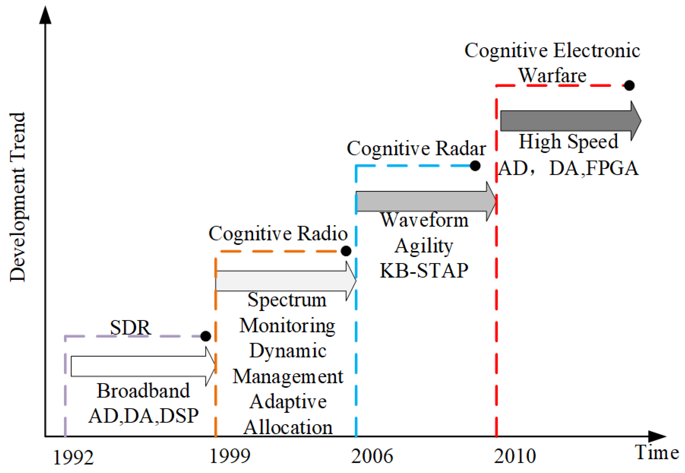
Figure 1, the development of CEW technology over the past few decades has benefited from the advancement and integration of multiple technologies. As a key component of CEW, radar jamming decision-making methods can be divided into two categories: traditional radar jamming decision-making methods and cognitive radar jamming decision-making methods.
1.2. Traditional Radar Jamming Decision-Making Methods
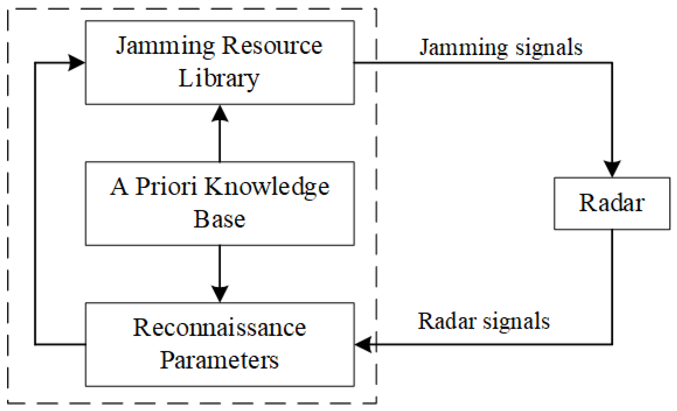
The traditional radar countermeasure model is shown in
Figure 2. The jamming system is only fixed according to the basic parameters of reconnaissance and an a priori radar database to call the jamming style of the jamming resource base. The system is unable to adjust the jamming method based on the jamming effect and environmental information, which would lead to inefficient jamming.
Currently, traditional radar jamming decision-making methods mainly include the following: game theory-based methods, template-matching-based methods and inference-based methods. David et al. [
17] proposed a framework that uses game theory principles to provide an autonomous decision-making for appropriate electronic attack actions for a given scenario. Gao et al. [
18] established a profit matrix based on the principle of minimizing losses and maximizing jamming gains and used a Nash equilibrium strategy to solve for the optimal jamming strategy. They relied on the establishment of the profit matrix, which is only applicable to radar systems with constant parameter characteristics. Sun et al. [
19] proposed an electronic jamming pattern selection method based on D-S theory. Li and Wu [
20] proposed an intelligent decision-making support system (IDSS) design method based on a knowledge base and problem-solving units. The method has wide applicability but relies too much on posterior probability and has poor real-time performance. Ye et al. [
21,
22] proposed a cognitive collaborative jamming decision-making method based on a swarm algorithm, which finds the global optimal solution through the process of searching for quality resources using a swarm. There are many similar population intelligence algorithms, such as genetic algorithms [
23,
24], ant colony algorithms [
25], differential evolutionary algorithms [
26,
27,
28] and water wave optimization algorithms [
29]. All these algorithms can be useful for solving jamming decision-making models, but the autonomy, real time use and accuracy cannot fully meet the requirements of CEW. These algorithms are mainly applicable to radars with constant feature parameters and rely heavily on adequate a priori information.
1.3. Cognitive Radar Jamming Decision-Making Methods
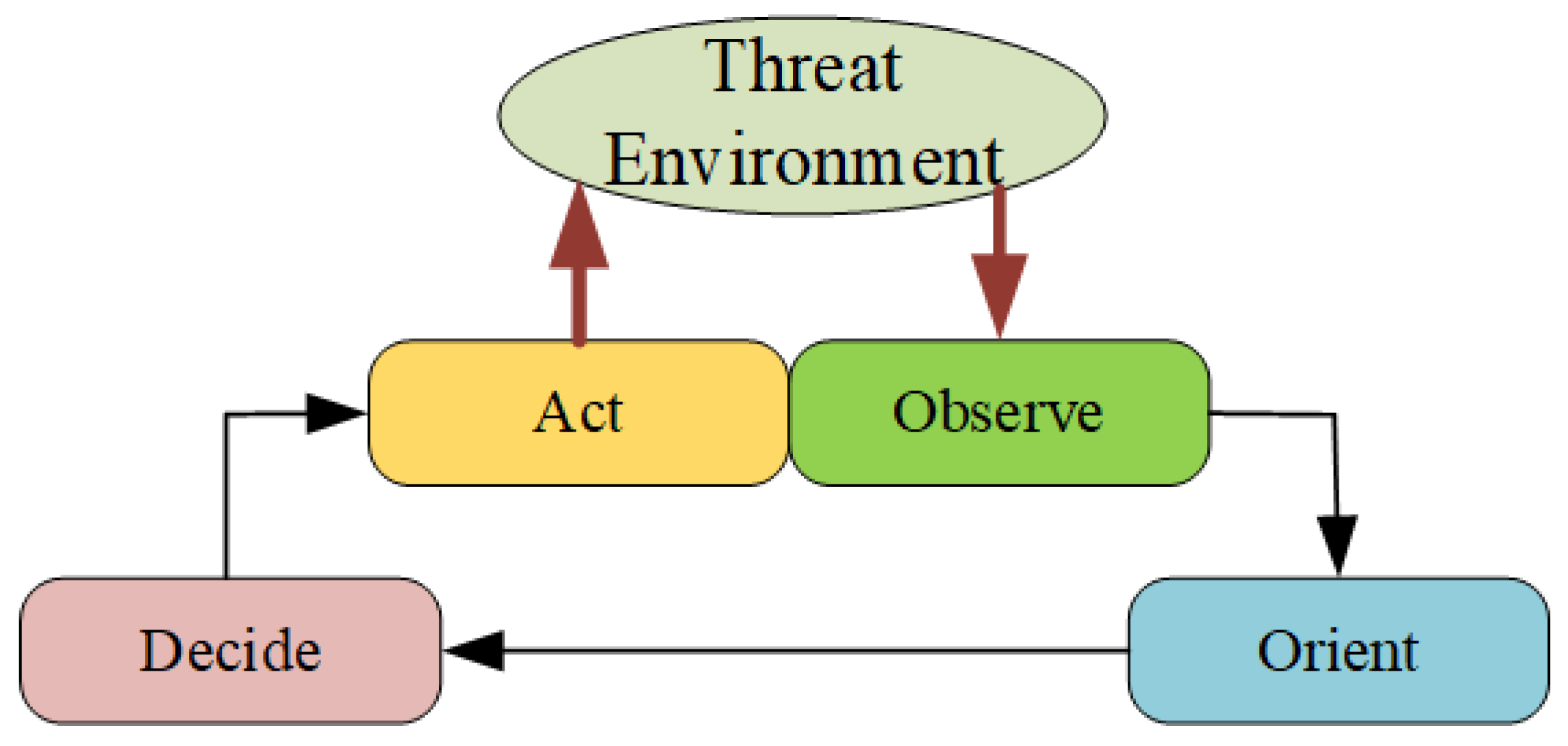
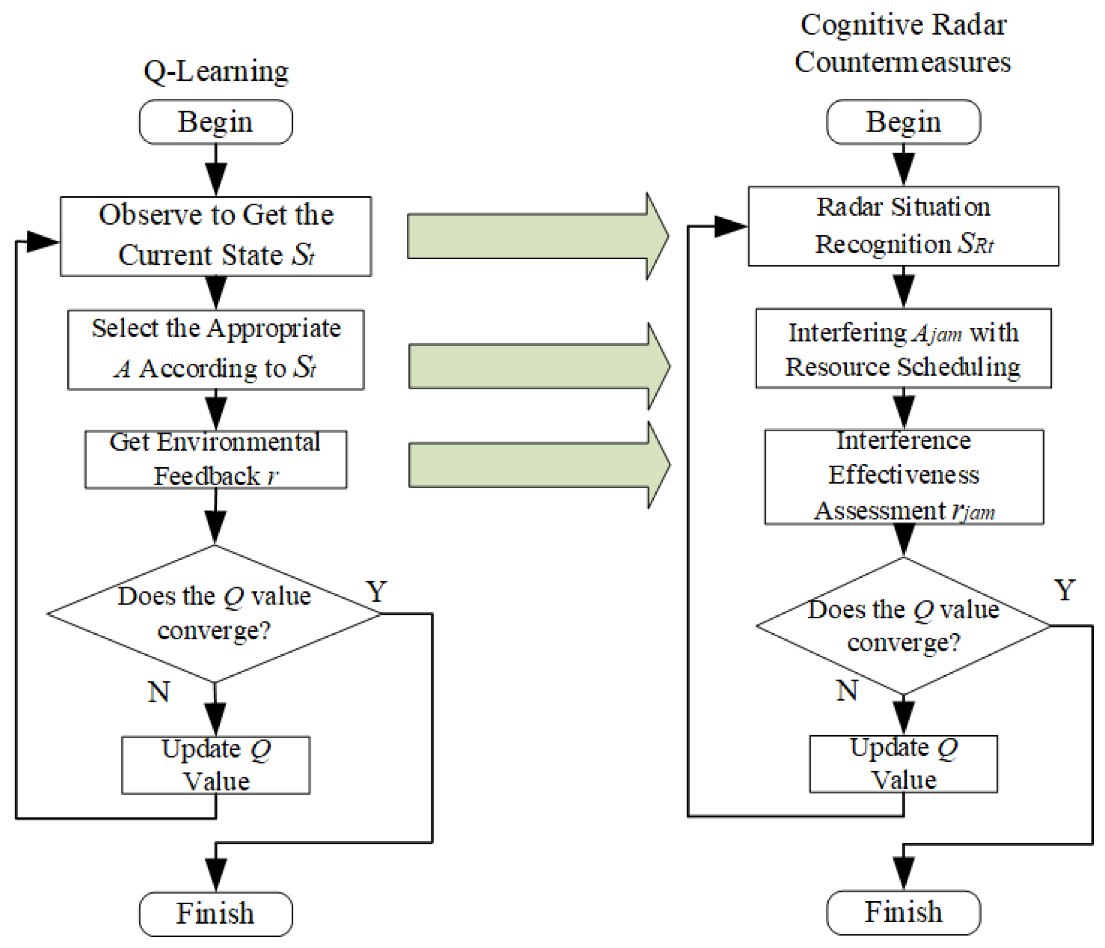
A CEW system can be defined as an Observe, Orient, Decide and Act (OODA) cycle with an adaptation capability (i.e., AI).
Figure 3 shows the working process of a typical OODA. The jammer first reconnoiters and sorts out the target signals from the threat environment system, then measures the parameters and identifies the target state. After the jammer adapts to the target state change, jammer evaluates the jamming efficiency, schedules jamming resources and optimizes jamming parameters to achieve effective jamming. The biggest difference between CEW and EW is that CEW and the environment can form a closed-loop system.
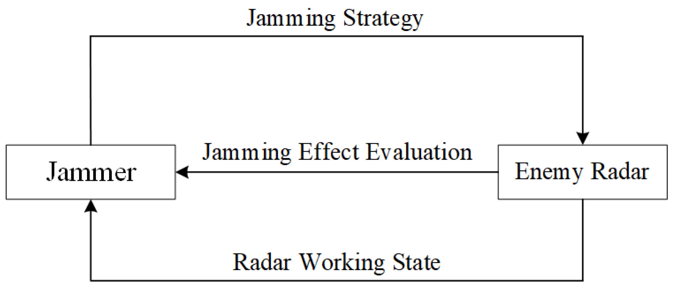
The cognitive intelligence of the agent is reflected in the process from cognition to memory, judgment, imagination and expression of the result. The cognitive radar jamming decision-making model is shown in
Figure 4. Its characteristics are as follows:
- (1)
Observe: The agent is able to perceive relevant information about the external environment and to obtain relevant information.
- (2)
Orient: The agent can use existing knowledge to guide thinking activities based on the perceived information.
- (3)
Decide: The agent is able to learn independently, interact with the external environment and adapt to changes in the external environment.
- (4)
Act: The agent is able to make autonomous decisions in response to changes in the external environment.
In the increasingly complex and changing electromagnetic environment, jamming and anti-jamming techniques are emerging. During countermeasures, the position between the radar and jammer dynamically changes, and power and distance greatly influence the effectiveness of different jamming styles. In this case, it is difficult to establish a one-to-one mapping between the specific working state of the radar and the available jamming techniques. At the same time, with the rapid development of new weapons and equipment, many new systems and multifunctional radars have emerged, and the jamming decision-making methods relying on a priori information and template matching are completely unable to adapt to current battlefield environments. Therefore, the research on intelligent radar jamming decision-making methods adapted to CEW has received much attention. CEW is a game process between two intelligences: the jammer and the radar. The research in this paper focuses on the countermeasure decision-making algorithm of the jammer.
Cognitive radar jamming decision-making has received extensive attention and development in recent years. Cognitive radar jamming decision-making is the ability to establish the best correspondence between radar and jamming styles in radar countermeasure systems through threat target awareness. Radar jamming decision-making based on the RL algorithm has been the focus of research in recent years. The RL algorithm generates the optimal strategy by continuously interacting with the environment [
30,
31].
The
Q-Learning algorithm is a typical time-series differential RL algorithm based on model-free learning. It enables the system to learn autonomously and to make correct decisions in real time without considering environmental models or prior knowledge [
32]. Therefore, compared with traditional jamming decision-making methods,
Q-Learning algorithm-based jamming decision-making methods can realize learning while fighting, which is expected to be a major research direction and future trend.
Q-Learning is currently widely used in robot path planning [
33,
34], nonlinear control [
35,
36] and resource allocation scheduling [
37,
38] and has yielded specific results in recent years for radar jamming decision-making. Xing et al. [
39,
40] proposed applying the
Q-Learning algorithm to radar countermeasures for the problem of unknown radar operating modes. The jamming system continuously monitors the state of the radar target, evaluates the effectiveness of the jamming, and feeds the results to the jamming decision-making module. Li et al. [
41] suggested using
Q-Learning to train the behavior of radar systems to achieve effective jamming and to adapt to various combat scenarios. Zhu et al. [
10,
42,
43] proposed applying the
Q-Learning algorithm to radar jamming decision-making for a particular multifunctional radar model and discussed the effect of prior knowledge and various hyperparameters on the convergence of the algorithm. From the simulation experimental results, it is known that by adding prior knowledge and adjusting the hyperparameters, the algorithm can improve the convergence speed and stability, and increase its robustness. Li et al. [
44] designed a radar confrontation process based on the
Q-Learning algorithm and verified the convergence of Q-values and the performance improvement in the algorithm through simulations using prior knowledge. Zhang et al. [
45] proposed the
DQN algorithm applied to radar jamming decision-making research for efficiency degradation caused by the increase in the number of target radar states. By comparing with the simulation experiments of the
Q-Learning algorithm, this method can better learn the effect of jamming in an actual battlefield autonomously and carry out jamming decision-making for multifunctional radars.
The
Q-Learning algorithm also has its shortcomings when applied. First, the practical application of
Q-Learning relies on several hyperparameters in the algorithm. Most of the existing results use a fixed exploration factor. When the exploration factor is large, the algorithm will explore sufficiently during the early stage and reach the optimal solution nearer quickly. However, it does not reach the convergence value effectively and oscillates at the optimal solution attachment, creating a difficult convergence situation. When the exploration factor is small, the algorithm does not explore sufficiently during the early stage and tends to fall into the local optimum during the later stage. Therefore, ensuring both exploration sufficiency and the stability of convergence using a fixed exploration factor is difficult. There are also no fixed rules for the learning rate and discount factor, which are generally set to fixed values by researchers through experience. When the learning rate is large, the algorithm is vulnerable to a learning risk early on. When the learning rate is small, the algorithm converges slower in the later stages. Secondly, the algorithm encounters problems such as slow and unstable convergence during the convergence process, which seriously affects the decision-making effect of the intelligent systems. Therefore, it is necessary to improve the
Q-Learning algorithm in order to improve the accuracy and efficiency of the
Q-Learning algorithm applied to radar jamming decision-making. Li et al. [
32] proposed an improved
Q-Learning algorithm that introduced the Metropolis criterion of a simulated annealing algorithm, which effectively solved the local optimum problem in the radar jamming decision-making process. Meanwhile, a stochastic gradient descent with the warm restarts method is used for the learning rate in the algorithm, which reduces the oscillations in the late iteration and improves the depth of convergence.
1.4. Research Focus
In today’s battlefield environment, multi-function radars are usually phased-array radars, which can simultaneously detect and identify targets in multiple states and directions. Using a single jammer as the jamming side is not effective in containing the radar’s threat. Additionally, a single jammer’s RL process will be slow when facing a radar operating in multiple states simultaneously. The longer it takes for the jammer to reach convergence, the higher the probability of the opposing radar detecting and destroying it. Therefore, clustered multiple jammers can achieve collaborative radar jamming decision-making with shared information. The clustered multiple jammers method has several advantages over using a single jammer, including the following:
- (1)
Convergence speed: Multiple jammers can converge more rapidly with target radars in multiple operating states during countermeasures, reducing the probability that individual agents will be detected and destroyed.
- (2)
Coverage area: Multi-functional radars operate in different states and orientations. Multiple jammers respond to the target radar in different orientations on the basis of information sharing.
- (3)
Hardware and power limitations: When jamming a single radar using a cluster of jammers, UAVs are often used as carriers for jammers. A single jammer requires higher requirements for power and hardware resources to implement effective jamming. Single-function jammers are overwhelmed by powerful multifunctional radars during confrontation and can be limited by distance, power and destruction. Moreover, a single jammer is often unable to operate in multiple states simultaneously due to its size and poor antenna isolation, among other reasons. Therefore, multiple jammers form clusters based on information sharing in order to achieve a greater advantage in an actual battlefield.
In response to the above problems, a radar jamming decision-making method Ant-QL based on the improved Q-Learning and ant colony algorithm is proposed in this paper. The algorithm includes the following:
- (1)
Explore strategy: The -greedy algorithm is introduced to change the search factor, thus balancing exploration and exploitation in the algorithm. This method ensures that the larger exploration factors can be fully explored during the early stage and the smaller exploration factors can reach the convergence state smoothly during the later stage of the algorithm.
- (2)
Pheromone mechanism: The Q-Learning algorithm converges slowly and tends to fall into local optima. To address the above problems, this paper introduces the pheromone mechanism of the ant colony algorithm into the Q-Learning algorithm to form an improved Q-Learning algorithm. The optimization process of the ant colony algorithm simulates the pheromone released by ants to explore the optimal solution. By combining Q-Learning with pheromones, not only is the reward value learned during the interaction between the agent and the environment but also the pheromone matrix for the transition between states is obtained. The pheromone as a path guide for the agent will make the convergence time of the agent shorter, while avoiding running into the local optimum.
- (3)
Termination conditions: In the convergence algorithm based on pheromone and Q-Learning during iteration, we use the Q-value convergence rule as the highest priority termination condition and the limit of the number of iterations as the next highest priority termination condition. After reaching the termination state, the algorithm outputs the optimal policy and the agent reaches the optimal state. In an actual battlefield environment, the jammer maximizes savings in terms of jamming resources and performs effective jamming.
- (4)
Advantages of cluster confrontation: We extend the confrontation between jammers and target radars to a cluster confrontation scenario to achieve the goal of collaborative jamming decision-making by multiple jammers against multifunctional radars. Cluster adversarial helps to reduce the need for hardware and a power system of individual jamming systems. Additionally, effective cooperative jamming can suppress a target radar in multiple airspace/time/frequency domains at the same time. During the adversarial process, the method reduces the convergence time, thus reducing the probability of the jammers being destroyed. At the same time, clustered jammers are more conducive to achieving effective countermeasures and ensuring our dominance in the radar countermeasure process.
- (5)
Termination conditions for cluster adversarial: Determining the termination state in the learning process of a cluster jammer is crucial. In this paper, we assume that each jammer works independently, and when all the jammers have completed one round of iterations, information such as the Q-value matrix and pheromones are shared, and the shared information of all the jammers is updated. This method can greatly accelerate the iteration speed and effectively improve the stability and robustness of the algorithm.
In this paper, we construct a multifunctional radar state transfer model with the number of states at 16 and the number of jamming modes at 10, drawing on the multifunctional radar model provided by [
46]. We propose an improved
Q-Learning algorithm and an
Ant-QL algorithm based on the ant colony algorithm. The conventional
Q-Learning algorithm and
DQN algorithm are simulated under the same decision-making model and used as comparison methods. After that, we perform simulation experiments on the improved
Q-Learning algorithm and
Ant-QL algorithm and compare them with the basic methods. The simulation results show that the new methods are useful for improving the autonomous learning efficiency of the jammer, shortening the response time of intelligent decision-making and greatly enhancing the adaptability of the jamming system.
The rest of the paper is structured as follows.
Section 2 details the traditional RL algorithm and the cognitive radar jamming decision-making model.
Section 3 describes the improved
Q-Learning and
Ant-QL algorithms in detail.
Section 4 gives the simulation experiments and the analysis of the results of four algorithms. Finally,
Section 5 discusses some conclusions drawn from this study and some future research hotspots and approaches in this area.
3. Improved Cognitive Electronic Jamming Decision-Making Method
3.1. Q-Learning Algorithm with Pheromone Mechanism
The jammer determines the difference in the threat level of the target by detecting changes in the working state of the enemy’s radar before and after the implementation of jamming. The jamming decision-making system learns the best jamming strategy through the jamming effect. Both the Q-Learning and DQN algorithms have real-time learning capabilities. Among them, the Q-Learning algorithm, as the core basic algorithm in RL, iterates in real time by building a Q-table and finally obtains a converged Q-value table. The disadvantage of the Q-Learning algorithm is that the hyperparameters, especially the variation in the exploration factor, have a great impact on the convergence. Usually, the setting of hyperparameters for the algorithm is empirically dependent. Q-Learning algorithms are less efficient when learning for large-scale states, and during radar confrontation, longer convergence times mean higher chances of being detected and destroyed. Additionally, the Q-Learning algorithm explores the suboptimal states repeatedly during the iterative process due to the certain randomness of action selection and the limited update magnitude of the Q-table elements. Due to the presence of neural networks, the DQN algorithm can cope better with the goal of a large state size. However, the complexity of the DQN algorithm is much greater than that of Q-Learning, including the hyperparameters of the network and the learning time. At the same time, the DQN algorithm suffers from an overestimation problem, which has a significant negative effect on the actual jamming decision-making. We have to improve the DQN algorithm to solve the overestimation problem, and the complexity and hyperparameters of the improved DQN algorithm will be improved. These situations are not favorable for our application in practice.
In this paper, we propose the Ant-QL algorithm to address the shortcomings of the existing typical Q-Learning and DQN algorithms. We introduce the pheromone mechanism of the ant colony algorithm in the Q-Learning algorithm. As a bio-inspired algorithm, the ant colony algorithm finds a path from the starting point to the end point that meets the conditional constraints by simulating the process of ants foraging for food.
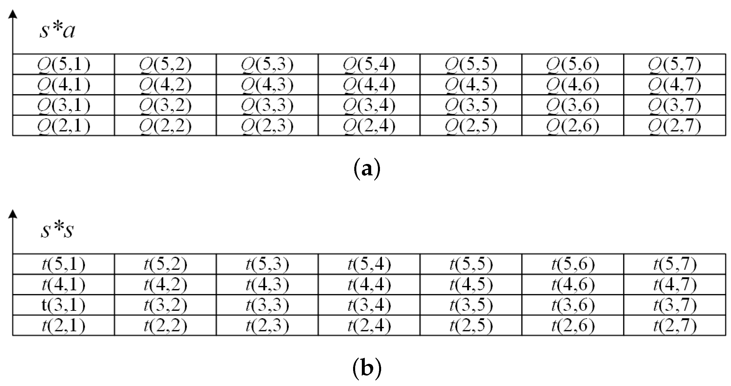
The essence of the cognitive radar jamming decision-making problem is that the jammer responds more effectively to the state transfer of the target radar. Ant colony algorithms are mostly used in problems such as optimization functions and path finding. As shown in
Figure 7, the core pheromone in the ant colony algorithm can be mapped to the Q-value table in the
Q-Learning algorithm. The Q table is initialized with
storage cells, where
s is the number of states and
a is the number of actions.
Figure 7a shows the structure of the Q-table. A pheromone table is generated according to the structure of the Q-table, as shown in
Figure 7b. During the iteration, the agent leaves pheromones in the pheromone table. As the pheromones are continuously updated, the strategy provided by the pheromone matrix to the agent becomes closer and closer to the optimal strategy.
The process of the
Q-Learning algorithm based on a pheromone mechanism is show in Algorithm 3. The improved
Q-Learning algorithm first initializes the Q matrix and all algorithm parameters. The agent first obtains the initial state from the environment. The agent performs an action to feed back to the environment. After the agent obtain the reward and the next state from the environment, the Q matrix is updated according to Equation (
3), where
is the pheromone value of the two states before and after the transfer. After each iteration, the jammer performs a global pheromone update. After several iterations, the distribution of pheromones becomes closer to the optimal path distribution. The pheromone update process is shown in Equation (
4), where
represents the pheromone value located at position
in the matrix at moment
t,
represents the pheromone value at the same position at the next moment and
is the pheromone change value. The calculation process of
is shown in Equation (
5), and the pheromone increase is obtained using the reward value and the number of iterations obtained from each loop.
| Algorithm 3 Improved Q-Learning algorithm. |
- 1:
Initialize , the number of iterations is N, the learning rate is , the discount factor is , the exploration factor , and the maximum number of single iterations is T - 2:
Initialize the pheromone matrix. - 3:
The reward value and number of each iteration, and the converged matrix. - 4:
for do - 5:
Get the initial state s. - 6:
for do - 7:
Select the action a in the current state s based on Q and pheromone matrix using the greedy strategy. - 8:
Get the feedback r, from the environment, and then update Q according to Equation ( 3). - 9:
end for - 10:
Update the pheromone matrix. - 11:
end for
|
3.2. Ant Colony Q-Learning Algorithm
In practical counter scenarios, it is difficult for a single jammer to have multi-antenna, wide range and high power jamming capabilities due to size and power limitations. The jammer is usually in a single orientation and frequency band during the countermeasure against the target radar, so it is difficult for it to perform jamming in multiple directions and in multiple frequency bands simultaneously. Additionally, the decision algorithm process for a single jammer means that no matter how it is optimized, a single jammer has a high chance of being detected and destroyed by the target radar compared with cooperative multi-machine jamming decision-making. Compared with traditional methods, the improved Q-Learning algorithm can converge to the optimal point faster and smoother and can effectively avoid becoming trapped in a local optimum. We can consider the Q-Learning algorithm with a pheromone mechanism as a single optimality-seeking intelligence (ant); then, the algorithm, when extended to a cluster, can be considered as a multi-intelligence (ant colony) algorithm. Multiple agents perform separate adversarial and decision-making processes in multiple working directions of the target radar; then, the radar jamming decision-making efficiency of the multi-agent remains relatively low. In this paper, we propose a multi-agent collaborative decision-making method based on information sharing. The method becomes simple in terms of hardware and power requirements and only requires the jammer to be able to cooperate in a single direction to achieve high-power suppression jamming. The target radar is usually considered to be able to perform a simultaneous operation in multiple dimensions and multiple frequency bands, but its state transition matrix is all consistent in the face of jamming. This is the key to the ability of multiple agents to cause effective cooperative jamming in decision-making.
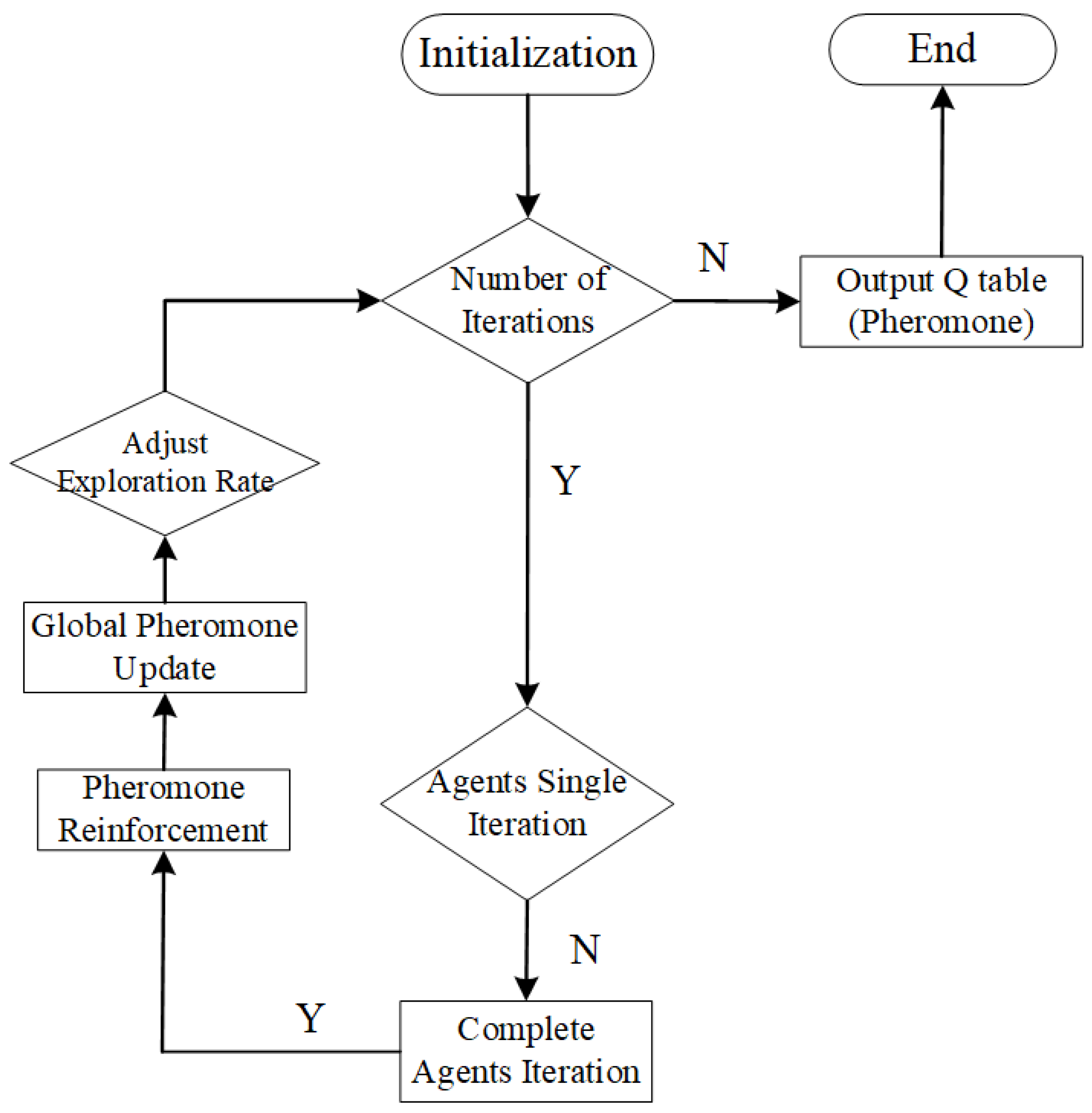
The flow of the cooperative jamming decision-making algorithm for multiple jammers is shown in
Figure 8. The initialization process includes the parameters of the
Q-Learning algorithm, the pheromone matrices and the number of agents. Here, the agents represent the jammers, and the number of agents is also the number of jammers. After all jammers complete one round of iterations, the increments in Q matrices (pheromone matrices) of some jammers with better effects are selected as shared information. The Q-matrices (pheromone matrices) of the less effective jammers are zeroed out and set as shared information. There are two differences in multi-machine jamming decision-making compared with single-machine jamming decision-making. The first is that the pheromone increase is calculated independently for each jammer, as shown in Equations (
6) and (
7). The evaporation mechanism of a pheromone needs to be considered in multi-machine jamming decision-making, and
in Equation (
6) is the volatilization factor. After several iterations, the algorithm can reach convergence faster and more stably. It should be noted that multiple jammers have different exploration steps at each round of iterations. During the simulation experiments, the Q matrix and the pheromone matrix stop updating after the jammer with a small number of exploration steps reaches the termination state. The jammer uses the existing Q matrix and pheromone matrix as a guide to interact with the environment. After all the jammers reach the termination state in this round, the algorithm selects the optimal agent in this round.
4. Simulation Experiments and Results Analysis
There will be various states of the radar during operation, such as search, tracking, identification, guidance, etc. There are also various jamming actions that can be performed by the jammer, such as noise FM jamming, false target jamming and distance dragging jamming. The state of a radar operation is denoted as
. The state of a jamming operation is denoted as
. States
,
and
represent the three search states. States
,
,
and
represent the four tracking states. States
,
,
and
represent the four identification states. States
,
and
represent the three guidance states. For the convenience of modeling, state
is set as the shutdown state and state
is set as the destroyed state in this paper. The jamming mode
represents noise amplitude modulation jamming. The jamming mode
represents noise FM jamming. The jamming mode
represents noise modulation jamming. The jamming mode
represents dexterous noise jamming. The jamming mode
represents dense dummy target suppression jamming. The jamming mode
represents distance deception jamming. The jamming mode
represents velocity deception jamming. The jamming mode
represents angle deception jamming. The jamming mode
represents distance–velocity deception jamming. The jamming mode
represents distance–angle deception jamming. The state transfer matrix is the working core of the target radar. Similar to Refs. [
42,
43], the state transfer matrices in this paper are set to empirical values. Additionally, the state of the radar and the threat level are positively correlated. During the simulation, the state transfer matrices are set with small fluctuations. When the target radar is subjected to some kind of suppression jamming, the table of transfer probability of radar operating state is shown in
Table 1. When the target radar is subjected to false target jamming, the state transfer matrix is shown in
Table 2. The state transfer matrices of the target radar when subjected to other jamming are not listed in this paper.
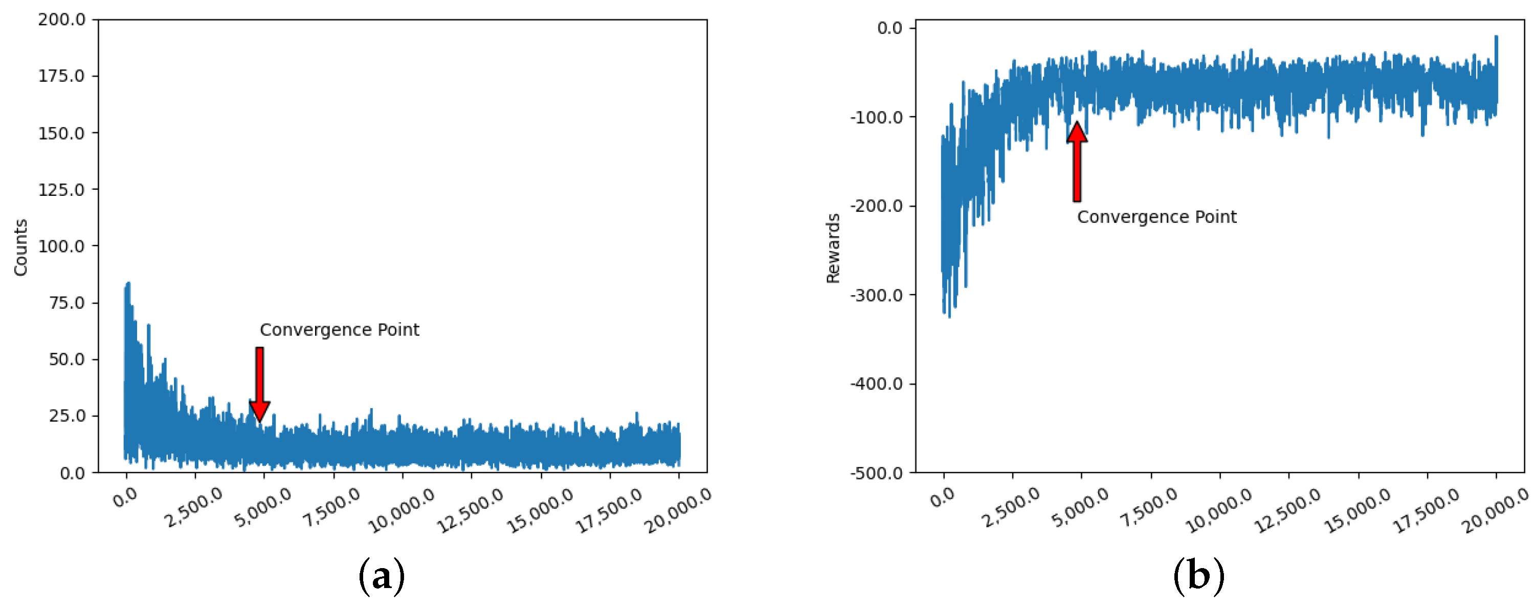
The parameters of the jammer with the Q-Learning algorithm are set as follows: the learning rate is 0.05, the discount factor is 0.7 and the initial value of the exploration factor is 0.99 and decreases with the number of simulation steps at a decay rate of 0.0003. The parameters for the DQN algorithm are set as follows: the learning rate is 0.01, the discount factor is 0.9, the initial value of exploration factor is 0.99,and the decreasing decay rate is 0.0003 with the number of simulation steps. The network in the DQN is a three-layer fully connected network, and the capacity of the replay buffer is set to 2000. The improved Q-Learning algorithm adds the pheromone-related parameters. The number of jammers for cluster jamming decision-making is assumed to be 3, i.e., three jammers collaborate with each other for jamming decision-making. All simulations are performed for 20,000 iterations. In this paper, the condition to end each round of iterations is that the radar state is transferred to the termination state or the number of explorations reaches 200. In the simulation experiments, we use the number of state transfers and the reward value in a single iteration as the quantitative evaluation criteria. It can be seen from the simulation results of multiple times that the convergence processes of both are completely synchronized and can confirm the convergence process with each other. The criterion for determining convergence in this paper is to divide every 10 iterations into groups. The average of the cumulative reward value and the number of state transfers is calculated for each group. The mean values between two adjacent groups are compared separately. We determine that the agent has reached convergence when the mean value of reward values in each group is less than −120 and the difference between the means of two adjacent groups is not greater than 15.
According to the convergence assessment criterion in this paper, we obtained the following results through simulation experiments. The simulation results of the
Q-Learning algorithm are shown in
Figure 9. As can be seen in
Figure 9a,b, they converge at the 4800th iteration.
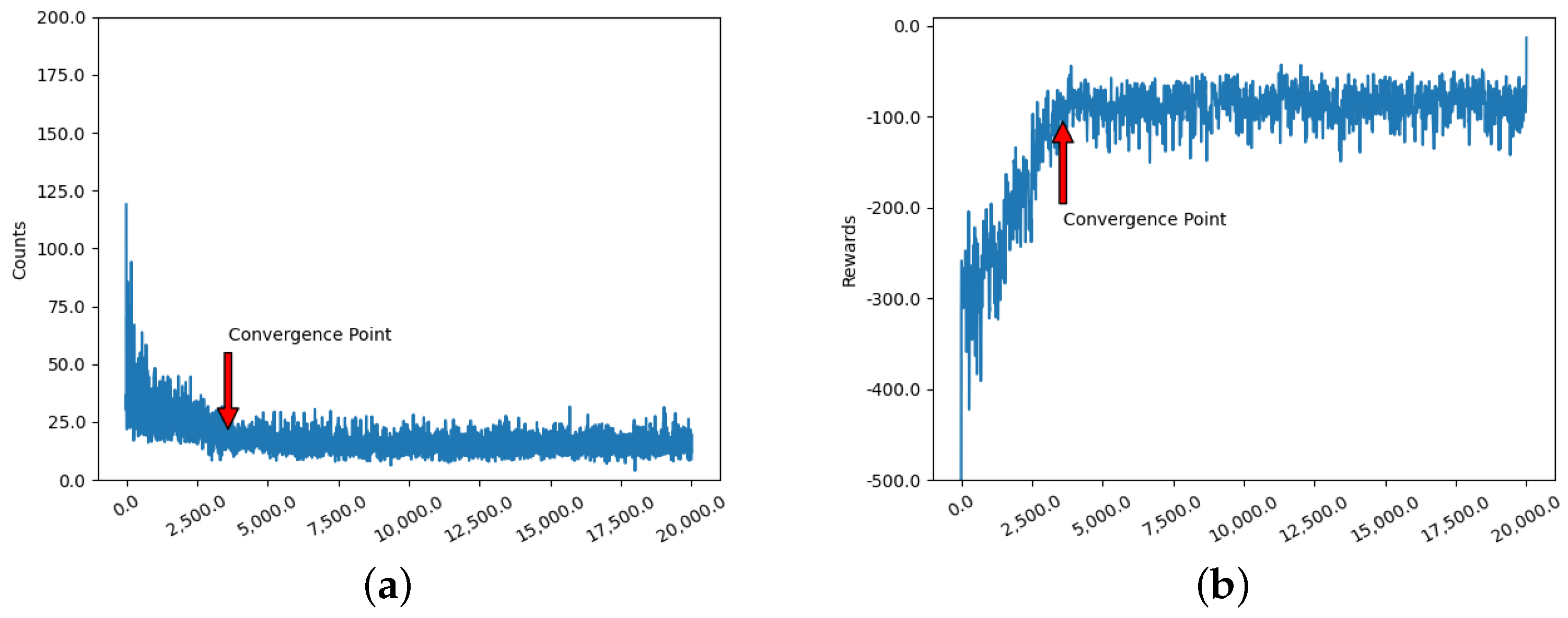
Figure 10 shows the simulation results of the
DQN algorithm, which converges at the 3600th iteration.
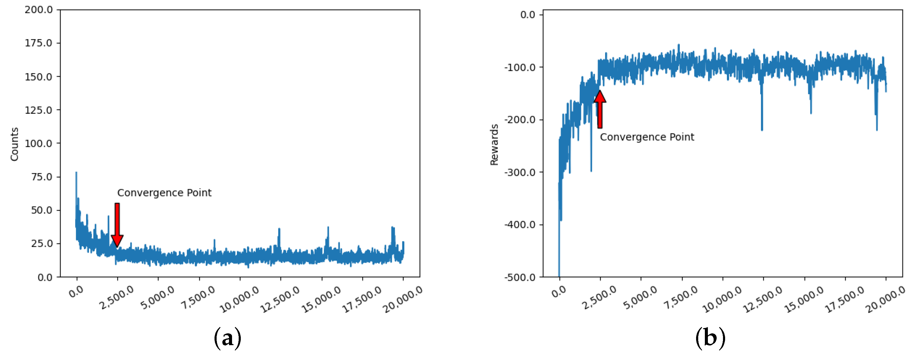
Figure 11 shows the simulation results of the improved
Q-Learning algorithm, which converges at the 2500th iteration.
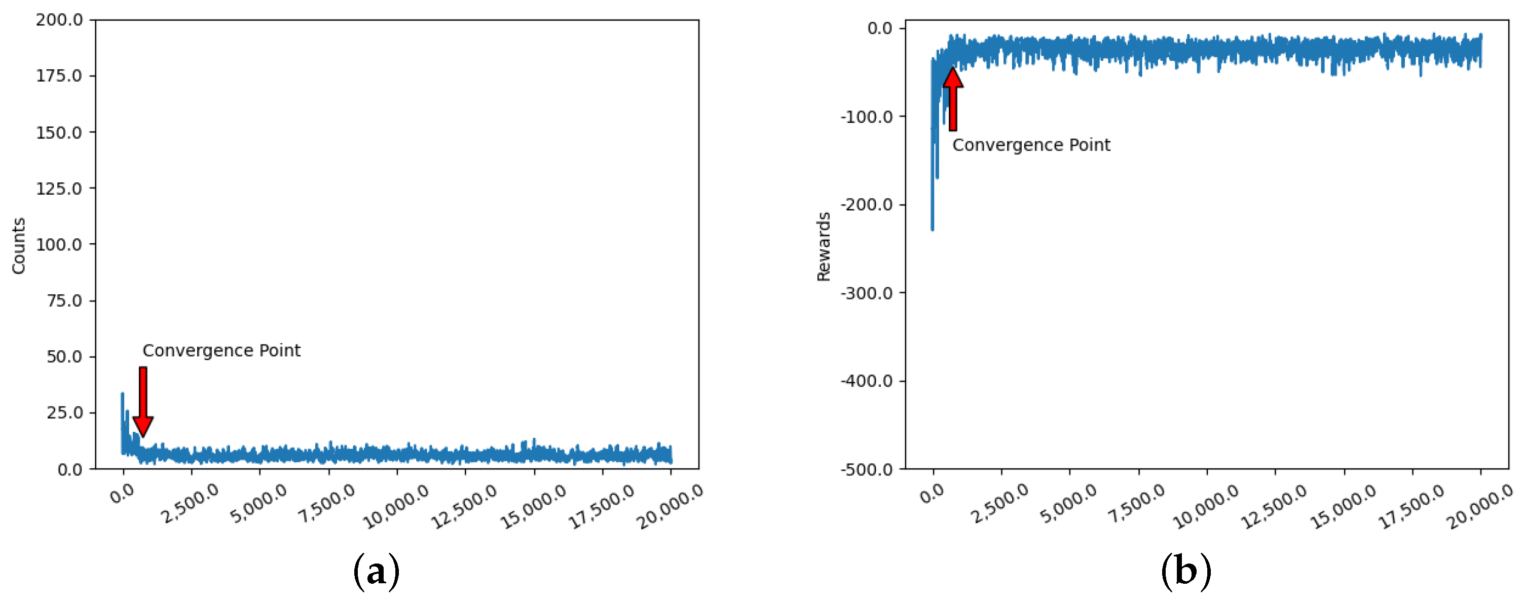
Figure 12 shows the simulation results of the
Ant-QL algorithm, which converges at the 700th iteration. The convergence results of the four different algorithms are shown in
Table 3.
After the simulation, it can be seen that the DQN algorithm accelerates the convergence speed and stability compared with the Q-Learning algorithm. However, the DQN algorithm suffers from the computationally time-consuming feature, which makes it difficult to achieve more desirable results. Comparing Q-Learning and DQN, the convergence speed of the improved Q-Learning algorithm is improved by 48% and 31%, respectively. The convergence speed of the Ant-QL algorithm is improved by 85.4%, 80.56% and 72% compared with the convergence speed of the remaining three algorithms. In addition, we can also learn from the simulation results of these algorithms that the overall stability of the Ant-QL algorithm is very high and the difference between groups is very small.
The performance of each algorithm depends not only on the number of rounds of convergence but also on its average response time. After the algorithms converged, we tested each algorithm 50 times and obtained their average response times.
Table 4 shows the average response times of the four algorithms after convergence. The
DQN algorithm has the longest average response time due to the time-consuming nature of training the network. Compared with the
Q-Learning algorithm, the improved
Q-Learning algorithm reduced the average response time by 68.38%. The
Ant-QL algorithm has the fastest average response time, which proves that the algorithm is more adaptable in electronic countermeasures.
The simulation results prove the superiority of the Ant-QL algorithm. Compared with Q-Learning, Ant-QL makes the iterative process of the jammer faster and more stable by introducing pheromones while avoiding the problem of a local optimum that can occur in the Q-Learning algorithm. Compared with DQN, Ant-QL does not overestimate during the iterative process, and the jammer has the path guidance provided by the pheromone as the number of iterations increases. Ant-QL is also considerably less complex than the DQN algorithm when it comes to algorithm debugging and application. After the algorithms converge, the average response time of the algorithms has a large impact on the performance of the jammer. The average response time of the improved Q-Learning algorithm is faster than that of the Q-Learning algorithm due to the advantage of pheromones in the merit-seeking process. The average response time of the Ant-QL algorithm is faster than that of the improved Q-Learning algorithm due to the addition of multi-machine collaboration. These advantages not only reduce the hardware requirements of the jammer but also increase its advantages in a real battlefield.
5. Conclusions
In this paper, we proposed an improved method combining the pheromone mechanism and the Q-Learning algorithm and applied it to radar jamming decision-making. The method not only performs Q-table updating and learning during the iterative process but also continuously optimizes the search range of the jammer to find the optimal state transfer and purposefully improves the convergence speed and stability. Through the simulation results, it can be analyzed that the improved Q-Learning algorithm can avoid the local optimum and reach convergence faster during the iterative process. The complexity and training time of the algorithm have significant advantages over DQN, which can effectively reduce the probability of being detected and destroyed in the actual battlefield. To better adapt to the trend of cluster confrontation in future warfare and to effectively overcome the hardware and power limitations of a single jammer, we extend the improved Q-Learning algorithm with multiple machines to cope with these trends. Under the condition of information sharing, the method introduces the idea of an ant colony and shares the information by selecting the better jammer during each iteration. The Ant-QL algorithm for clustering reduces the hardware and power requirements of the jammer. The simulation results show very good convergence and stability, which will help to improve the survivability and adaptability of these jammers. Additionally, after the convergence of each algorithm, their average response times are discussed in this paper. The simulation results show that the improved Q-Learning algorithm and Ant-QL algorithm have shorter average response times compared with traditional methods.
CEW is receiving more and more attention. For cognitive radar jamming decision-making, there is also a continuous need to explore better algorithms. RL and metaheuristic algorithms are still a hot topic for many researchers, and new and various algorithms are emerging. This paper concludes with a few possible research points that will hopefully be useful to future researchers.
- (1)
Due to the increasing complexity of the battlefield situation, multi-UAV cluster reconnaissance positioning has gained tremendous attention and development [
50,
51]. The advantages of UAV clusters in reconnaissance and positioning are enormous, and there are still many technical difficulties waiting to be broken through.
- (2)
The research method in this paper has achieved better results, but there are still some problems. To address these problems, we also propose some new research plans. For example, if we increase the anti-jamming capability of the radar, the cooperative decision-making method of multiple jammers can be improved, for example, how to communicate efficiently between multiple jammers. It should also be noted that the Ant-QL method proposed in this paper discards information matrices that do not work well in each round. In the next stage of research, we need to consider how to utilize all information matrices of multiple jammers more effectively.
- (3)
For radar jamming decision-making, the jammers use hierarchical RL algorithms for radar jamming decisions in response to the hierarchical structure of the target radar. For increasingly urgent cluster confrontation, multi-jammers use multi-intelligence RL algorithms for radar jamming decision-making. There are limitations in using a single algorithm to solve this problem, and we hope that more researchers will combine algorithms such as metaheuristics with RL to solve this problem more effectively.
- (4)
Research on various new jamming methods is the key to gaining battlefield advantages. Radars of different regimes have many counterpart anti-jamming measures to traditional jamming methods. We note that the use of many new types of jamming usually achieves unexpected results [
52,
53,
54,
55].
- (5)
With the development of a cognitive radar, radar jamming decisions based on fixed jamming methods still pose a significant battlefield threat. A future jammer should be centered on radar jamming decision-making and have an adaptive jamming waveform optimization capability. These features will greatly enhance the flexibility and adaptability of jammers in the actual battlefield. Numerous meta-heuristic optimization algorithms are currently available for jamming waveform optimization [
56,
57].
- (6)
As battlefield complexity rises, electronic countermeasures in various clusters will proliferate. The jammer itself is limited by the resources of the applicable platform and often does not have the software, hardware and power resources to match the target radar. For the jamming side, the rational allocation of jamming resources to maximize operational effectiveness is the difficulty. Despite jamming waveform optimization, the jammer of the cluster needs to have a strong jamming resource scheduling algorithm. The algorithms currently applied to jamming resource scheduling include the Hungarian algorithm, the dynamic planning algorithm, etc. [
58,
59]. We believe that the fusion algorithm of a metaheuristic algorithm and RL is an effective method to realize cognitive electronic countermeasures in the future.


