Article

A Disturbance Frequency Index in Earthquake Forecast Using Radio Occultation Data

1
Computational Transport Phenomena Laboratory, Physical Science and Engineering Division (PSE), King Abdullah University of Science and Technology (KAUST), Thuwal 23955-6900, Saudi Arabia
2
National Space Science Center, Chinese Academy of Sciences, Beijing 100190, China
3
Beijing Key Laboratory of Space Environment Exploration, Chinese Academy of Sciences, Beijing 100190, China
4
Joint Laboratory on Occultations for Atmosphere and Climate, National Space Science Center, Chinese Academy of Sciences, Beijing 100190, China
5
Key Laboratory of Science and Technology on Space Environment Situational Awareness, Chinese Academy of Sciences, Beijing 100190, China
6
School of Astronomy and Space Science, University of Chinese Academy of Sciences, Beijing 100049, China
7
School of Petroleum Engineering, China University of Petroleum (East China), Qingdao 266580, China
8
National-Local Joint Lab for Bigdata Analysis and Computing Technology, Beijing 100811, China
9
School of Civil and Resources Engineering, University of Science and Technology Beijing, Beijing 100083, China
*
Author to whom correspondence should be addressed.
These authors contributed equally to this work.
Remote Sens. 2023, 15(12), 3089; https://doi.org/10.3390/rs15123089
Submission received: 5 May 2023 / Revised: 22 May 2023 / Accepted: 24 May 2023 / Published: 13 June 2023

Abstract

:
Earthquake forecasting is the process of forecasting the time, location, and magnitude of an earthquake, hoping to gain some time to prepare to reduce the disasters caused by earthquakes. In this paper, the possible relationship between the maximum electron density, the corresponding critical frequency, and the occurrence of earthquakes is explored by means of radio occultation data based on mechanism analysis and actual earthquake-nearby data. A new disturbance frequency index is proposed in this paper as a novel method to help forecast earthquakes. Forecasting of the location and timing of earthquakes is based on the connection between proven new frequency distributions and earthquakes. The effectiveness of this index is verified by backtracking observation around the 2022 Ya’an earthquake. Using this index, occultation data can forecast the occurrence of earthquakes five days ahead of detection, which can help break the bottleneck in earthquake forecasting.

Graphical Abstract

1. Introduction

Radio occultation is a remote sensing technique for measuring the physical properties of planetary atmospheres. It relies on detecting changes in radio signals passing through the planet’s atmosphere that are masked by the atmosphere. When electromagnetic wave radiation passes through the atmosphere, it is refracted, and the size of the refraction depends on the refraction gradient of the normal path, that is, the refractive index gradient depends on the density gradient. The effect of the influence is most pronounced when the radiation travels through a long path to the edge of the atmosphere. Figure 1 illustrates radio occultation measurements. LEO denotes Low Earth Orbit, and GNSS denotes Global Navigation Satellite System. Signals from GNSS satellites pass through the atmosphere and are received by LEO. Due to the existence of the earth, the signal cannot pass through the interior of the earth. Thus, only when GNSS and LEO satellites satisfy a certain geometric relationship can signals be received along the propagation path; otherwise, they will be blocked by the earth. Since both LEO and GNSS satellites are in constant motion, the geometric relationship between the satellites is also constantly changing over time. The moment the LEO satellite receives the signal from the GNSS satellite, marked as t1 in Figure 1, until the signal is obscured by the earth and cannot be received, marked as t2, is a process known as an occultation event [1].
In an ideal vacuum environment, the signal propagation path is a straight line [2], so the phase delay is directly related to the straight-line distance between the GNSS satellite and the LEO satellite. However, due to the existence of the earth’s atmosphere in the actual observation environment, a certain degree of bending may occur within the signal propagation path [3]. As a consequence, the distance of the propagation path changes due to the bending of the signal, which leads to a difference between the phase delay of the actual received signal by the LEO satellite and the phase delay in the case of straight-line propagation. Such delay is defined as Excess Phase Delay, also known as EPD [4]. If the electron content in the signal propagation path is high, the phase velocity of signal propagation will be greater than its propagation velocity in vacuum, resulting in a possible negative EPD value; otherwise, the EPD value will be positive [5]. Moreover, the size of the signal bending angle reflects the degree of influence of the atmosphere during the signal propagation process. It is directly related to the density of the substances at the height of that atmosphere. As a result, we can inversely estimate the distribution of such substances in the atmosphere based on the bending angle or additional phase delay of the signal [6].
Figure 2 shows the geometry at an instant in the occultation event. O represents the center of refraction of the occultation path, which coincides with the geometric center of the earth under the premise of spherical approximation [7]. The angle between (OL) and (OG) is defined as θ, and the plane formed inside is called the occultation plane [8]. In this plane, the (GT) direction is the transmitting direction of the signal, the (TL) direction the receiving direction, and the angle between them is called the bend angle of the occultation path, α, which reflects the degree of curvature of the signal propagation path [9]. A positive value means it is curved to the outside (that is, the side away from the earth), and a negative value means that it is curved to the inside (that is, the side closer to the earth). The red solid line in Figure 2 represents the actual propagation path of the signal in the atmosphere, and the red dotted line represents the ideal propagation path in a vacuum environment. OP and OQ are perpendicular to the direction of signal transmission and reception, respectively, and their length p is called the impact parameter [10]. M is the closest point on the signal propagation path to the earth’s surface, which is called the perigee of the occultation event or the occultation event tangent point [11].
Due to the difference in the content and distribution of substances at different heights in the atmosphere, the signal refractive index at different heights also varies [12]. Therefore, in the process of GNSS signal propagation, with the change in the height of the signal, signal refraction and path bending continuously occur. For the convenience of explanation and analysis, the bending angle α shown in Figure 2 is actually the summation of the bending degrees caused by all refractions in the signal propagation path. An occultation event generally lasts from several minutes to more than ten minutes [13], and at each instant, there will be an occultation path with the geometric relationship shown in Figure 2, as well as a perigee in each occultation path. What we are concerned with is the atmospheric parameters corresponding to the heights of the near points in this observation sequence. In an occultation event, with the relative motion of the GNSS and the LEO satellite, the perigee height of the signal propagation path will also change accordingly, and finally, a scan of the vertical profile of the atmosphere is completed. According to the characteristics of perigee height variation in occultation events, we call the occultation event with perigee height from low to high an ascending occultation event, and the occultation event with perigee height from high to low is called a descending occultation event [14].
Satellite monitoring has broken through the limitations of traditional seismic scientific research, and electromagnetic waves can propagate across spheres from underground to space. Statistics show that there is a significant correlation between spatial electromagnetic disturbances and earthquake occurrence. Scientists can expand their observation range to the global scale through satellites. From the perspective of earthquake observation and collection, satellite monitoring can enable scientists to conduct large-scale statistical research, providing a foundation for testing various methods and models. With the capability to capture ionospheric perturbations, radio occultation is expected to play a role in earthquake forecasting. Earthquake forecasting has always been a global challenge, mainly due to scientists’ lifelong difficulties in accumulating enough destructive earthquake cases to form statistics and validate forecast methods and theories [15]. The possibility of using ionospheric perturbations to recognize processes, which occur at the earth’s surface and inside the crust prior to major earthquakes, has been focused on in past decades in terms of effectiveness, adaptability, and reliability [16,17]. If the risk of earthquake occurrence can be predicted ahead of when it happens [18] and the phenomenon indicating the occurrence can be recognized [19], more time can be gained to better protect us from the disaster [20]. Generally, ionospheric anomalies are believed to be more significant for strong earthquakes, as pointed out in [21] (M ≥ 6.0), [22] (M ≥ 5.5), and [23] (M ≥ 4.6). Starting from the pioneering work reported in [24], scientists have been devoted to figuring out an index that can directly represent the correlation between earthquakes and ionospheric anomalies [25,26]. The total electron content was focused on in [27] as an index after analyzing the GPS data observing the Northbridge earthquake [28]. After that, the electron content was regarded as a potential precursor index in various strong earthquakes, including the 2008 Wenchuan earthquake [29,30] and a number of M ≥ 6.0 earthquakes in East Asia [31,32]. Another characteristic of the ionospheric anomaly is that the anomalous amplitude increases with the decrease in latitude; that is, the anomalous peak has a tendency to drift to the magnetic equator [33]. In the low-latitude region, due to the special geomagnetic and electrodynamic environment, the seismic ionospheric effect changes the distribution of the equatorial anomaly as a whole within a certain longitude range; that is, the double peak of the ionospheric anomaly has a tendency to drift to the magnetic equator [34].
However, considering the strong daily variation of the ionosphere that may be detected even in the period when the geomagnetic field is very calm [35], the reliability of using electron density as the sole index is challenged [36]. This paper analyzes and studies the precursor phenomena that may be related to earthquakes and explores an index as an earthquake precursor using occultation observation. The remainder of this paper is organized as follows. In Section 2, we investigate the inverse algorithm in ionospheric occultation that can help us obtain measurement data. The technical details of the algorithm are listed in the appendixes. The seismo-ionospheric monitoring mechanism is reviewed in Section 3, indicating the potential indexes that may be relevant to earthquakes. A case study of the 2022 Ya’an earthquake is investigated in Section 4. The spatial and temporal change in the maximum electron density and the corresponding critical frequency around the earthquake is illustrated. A novel disturbance frequency is proposed based on the two factors to perform the role of a quantitative index that can be used to forecast the time, location, and magnitude of an upcoming earthquake. The effectiveness of this index is validated. Concluding remarks are provided in Section 5, analyzing the limitations of the current approach and suggesting future developments, including the application of deep learning algorithms.

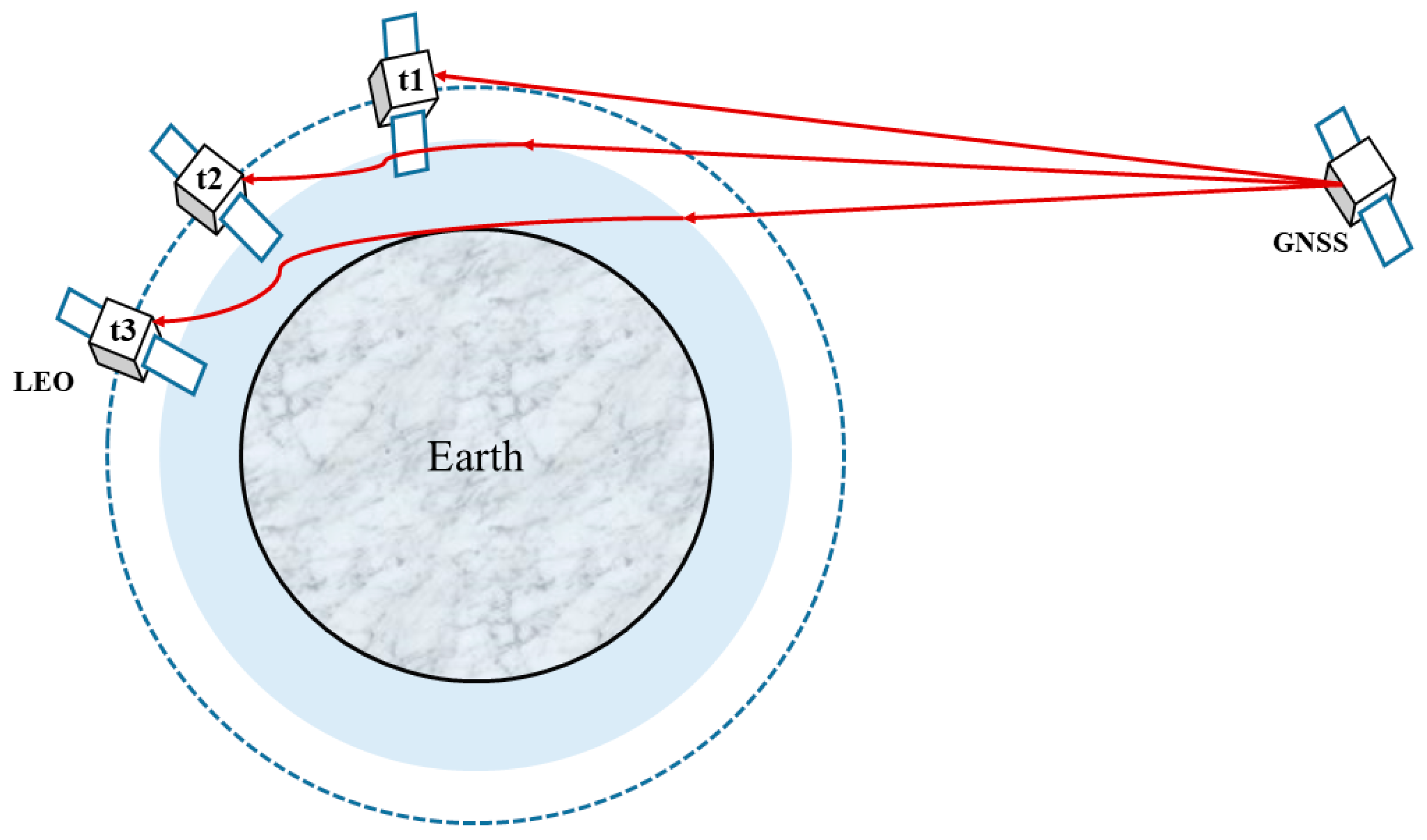
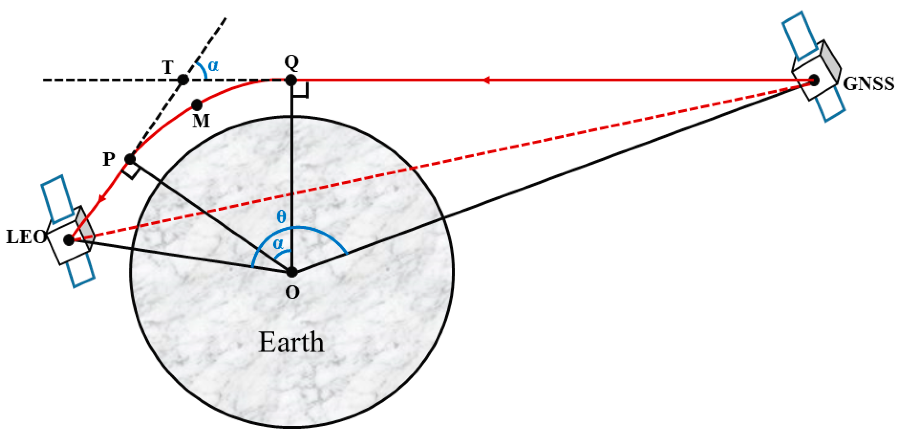
2. Inverse Algorithm in Ionospheric Occultation

2.1. Data Preprocessing

Before performing ionospheric occultation inversion, some necessary preprocessing of the observation is required to prepare for the formal inverse calculations to improve the reliability of the inversion results. The detailed processing flow can be seen in Appendix A.

2.2. Doppler Inverse Algorithm

The basic idea of the Doppler-based occultation inverse algorithm is to obtain the additional Doppler frequency shift by deriving the additional phase delay with respect to time. According to the Doppler principle and the instantaneous geometric relationship of the occultation, the impact parameter and bending angle sequence can be obtained, the refractive index profile can be calculated by combining the Abel integral, and finally, the electron density profile can be obtained by further inversion using the relationship between the refractive index and the electron density. The input information of this method is the additional phase delay of ionospheric occultation data, the spatial coordinates and speed of GNSS and LEO satellites, and the UTC time of the observation moment, and the output information is the electron density profile of the ionosphere, the perigee latitude and longitude, and the UTC time. The technical details of the Doppler inverse algorithm are given in Appendix B.

2.3. TEC Inverse Algorithm

TEC, short for Total Electron Content, is an important descriptive quantity for the ionosphere of the earth. The TEC is the total number of electrons integrated between two points, along a tube of a one-meter-squared cross-section, i.e., the electron columnar number density. The basic idea of the TEC-based occultation inverse algorithm is to calculate the TEC on the signal propagation path through the additional phase delay and directly calculate the impact parameter corresponding to each occultation moment under the assumption of linear propagation. The TEC sequence is derived with respect to the impact parameter, and the electron density profile can be obtained by inverting the obtained TEC differential sequence by Abel integration. The input and output information of the TEC-based occultation inversion algorithm is basically the same as that of the Doppler-based occultation inversion algorithm. The difference is that the bending angle of the ionospheric occultation is generally very small, and the signal propagation path is approximated as a straight line in this inverse process. More details of the inverse TEC algorithm can be seen in Appendix C.

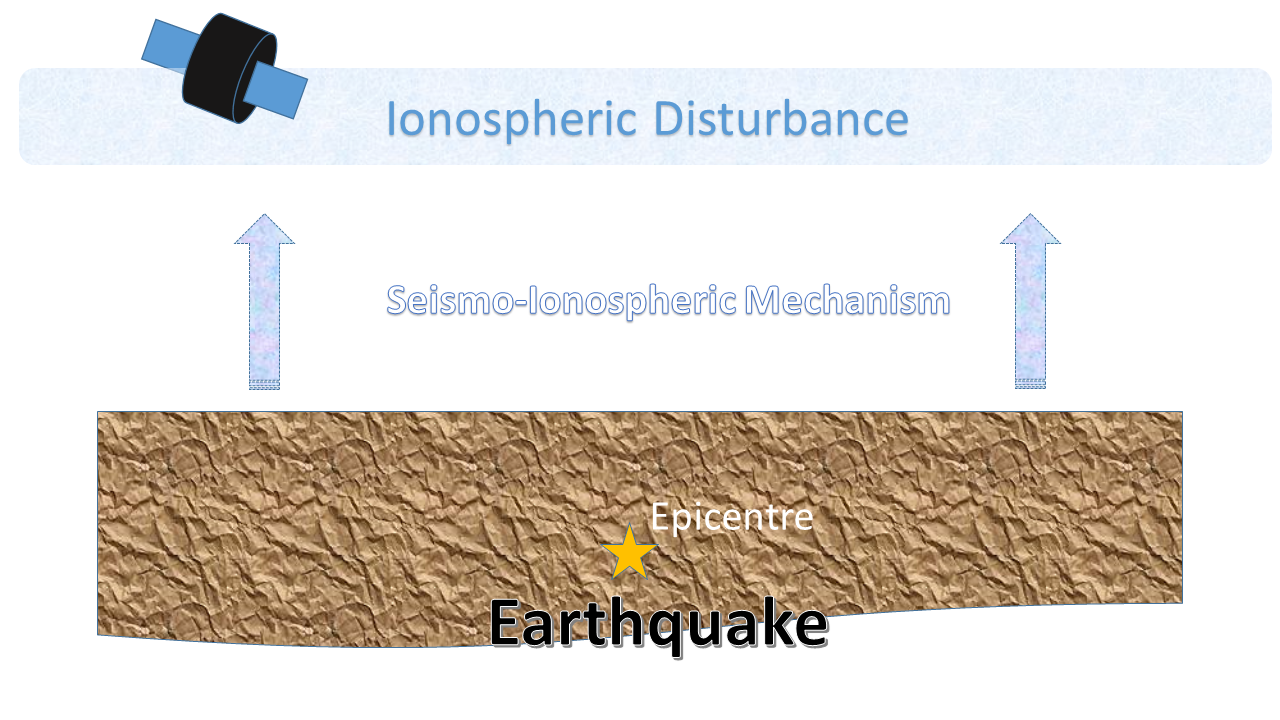
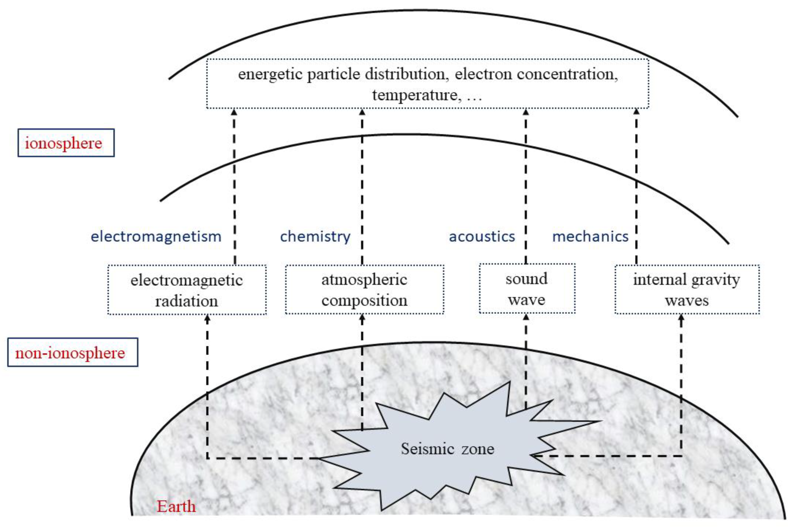
3. Seismo-Ionospheric Monitoring Mechanism

In 2004, the successful launch of the DEMETER (Detection of Electric-Magnetism Emissions Transmitted from Earthquake Regions) satellite to detect the seismic ionospheric effect announced a new period of space-based seismic electromagnetic observation [37]. Using GIM (Global Ionospheric Map) data released by the JPL (Jet Propulsion Laboratory), it was analyzed in [38] that TEC anomalies before the 2008 Wenchuan MS8.0 earthquake and an obvious increase in TEC were detected in the eastern–southern region of the earthquake. The TEC perturbation characteristics of 56 earthquakes of magnitude 6.0 or higher in China from 1998 to 2012 were studied in [39], and it was found that synchronous disturbances were observed in the magnetic conjugate region of the southern hemisphere. It was found that the TEC 2 to 9 days before the earthquake showed a rapid decline in the afternoon anomaly, which is similar to the seismic TEC disturbances in Indonesia and Taiwan Island at low latitudes.
One of the difficulties in short-term earthquake forecasting is that the earthquake mechanism is not clear [40]. Various related electromagnetic effects of earthquakes have not yet been uniformly expounded. In recent years, the scientific community has confirmed that there are electromagnetic coupling processes in the crust and troposphere in the corresponding active regions, and there are abnormal changes in the ionosphere in the days to hours before the occurrence of strong earthquakes, volcanoes, and tsunamis [41]. The many hypotheses that have been proposed to explain the seismo-ionospheric disturbance can be classified into the following two types [42]. One is the fluctuation of the ground or sea surface caused by the earthquake fault, which drives the generation of acoustic and gravitational waves in the atmosphere, and the other is that with the propagation of seismic waves (mainly Rayleigh waves), infrasound waves in the atmosphere are excited wherever the seismic waves go. An ionospheric disturbance caused by atmospheric fluctuations propagates from the epicenter to the periphery, with typical velocities ranging from a few 100 to 1000 m · s 1 , which is determined by the speed of acoustic or gravitational waves in the atmosphere and ionosphere. The ionospheric disturbance excited by the second mechanism follows the propagation of the Rayleigh wave, showing the same speed as about 3~4 km · s 1 . The schematic diagram of various hypotheses of seismic ionospheric disturbance mechanism is shown in Figure 3.
As shown in Figure 3, the change in the Total Electron Content (TEC) and other indexes can be detected in the ionosphere to help the earthquake forecast, and the mechanisms underneath such phenomena can be explained in a variety of subjects [43,44]. From the perspective of electromagnetism [45], the ULF (Ultra-Low Frequency) electromagnetic radiation generated in the lithosphere is generated before the earthquake and is introduced into the inner magnetosphere. After interacting with the energetic particles, the particles settle to the bottom of the ionosphere, causing ionospheric disturbance. From a chemistry point of view [46], in the seismic zone before the earthquake, there are radioactive geochemical phenomena, including the radiation of several gas components such as radon radiation and noble gas. Changes in geochemical parameters lead to changes in atmospheric compositions, which further enhances changes in atmospheric conductivity and atmospheric electric field. The appearance of this local electric field anomaly leads to changes in the electron density, ion composition, and electron temperature of the ionosphere. From an acoustic point of view [47], in the seismically active zone, the sound wave is disturbed by the gravitational vibration to produce an AGW (Acoustic Gravity Wave), which continues to propagate upward, resulting in the enhancement of gravitational waves and planetary waves, disturbing the ionosphere, and changing the ionosphere and the density of the plasma. From a mechanical point of view [48], in the seismogenic zone, due to the plate tectonics of the crust, the amplitude of gravity oscillations caused by seismic activity increases with the height from the ground. These kinds of piston movements affect the atmosphere and produce an IGW (Internal Gravity Wave). Due to the large vertical velocity of the IGW, it still has high energy when it propagates to the ionosphere, which makes the neutral compositions of the ionospheric plasma change and causes ionospheric disturbance. In this paper, we focus on generating a quantitative index based on the ionospheric disturbance that can be used as an indicator for forecasting the upcoming earthquake. The other mechanisms may be considered in future studies to formulate other indexes that can also help forecast earthquakes.

4. Disturbance Frequency Index in Earthquake Forecasting

4.1. 2022 Ya’an Earthquake Data

On 1 June 2022 (UTC + 8 time zone), two earthquakes occurred consecutively in the Ya’an area of Sichuan, China. The earthquake was a surface-wave magnitude (Ms) 6.1 earthquake (moment magnitude, Mw, as 5.8) that occurred at 17:00 on 1 June, local time, in Lushan County, Ya’an City, Sichuan Province (30.37 north latitude, 102.94 east longitude), with a focal depth of 17 km. In order to evaluate the effectiveness of radio occultation in earthquake forecasts, the COSMIC data around the 2022 Ya’an earthquake are collected and analyzed to investigate the possible indexes that may help forecast the occurrence of the earthquake. Using the Dobrovolsky formula [49], R = 10 0.43 M , where R denotes the radius of the earthquake preparation zone and M is the earthquake magnitude, the impacting radius of the 2022 Ya’an earthquake can be calculated as 419.76 km. Thus, the data were collected within a distance of 500 km from the epicenter. From 10 May 2022 to 19 June 2022, totally, 200 radio occultation events were recorded within this range during the 40 days around the earthquake. From the inverse algorithm described in Section 2 and the mechanism analysis in Section 3, two radio occultation indexes, namely the maximum electron density and the critical frequency at maximum electron density, are believed to be the main indexes that can be observed with obvious differences around the earthquake. The statistical information of the two indexes in the data are listed in Table 1. A rough guess can be referred from Table 1 that there exists abnormally large density in the profile, which makes the mean density significantly larger than the median value. Thus, the anomalies in the maximum electron density index might be an indicator of earthquake occurrence.

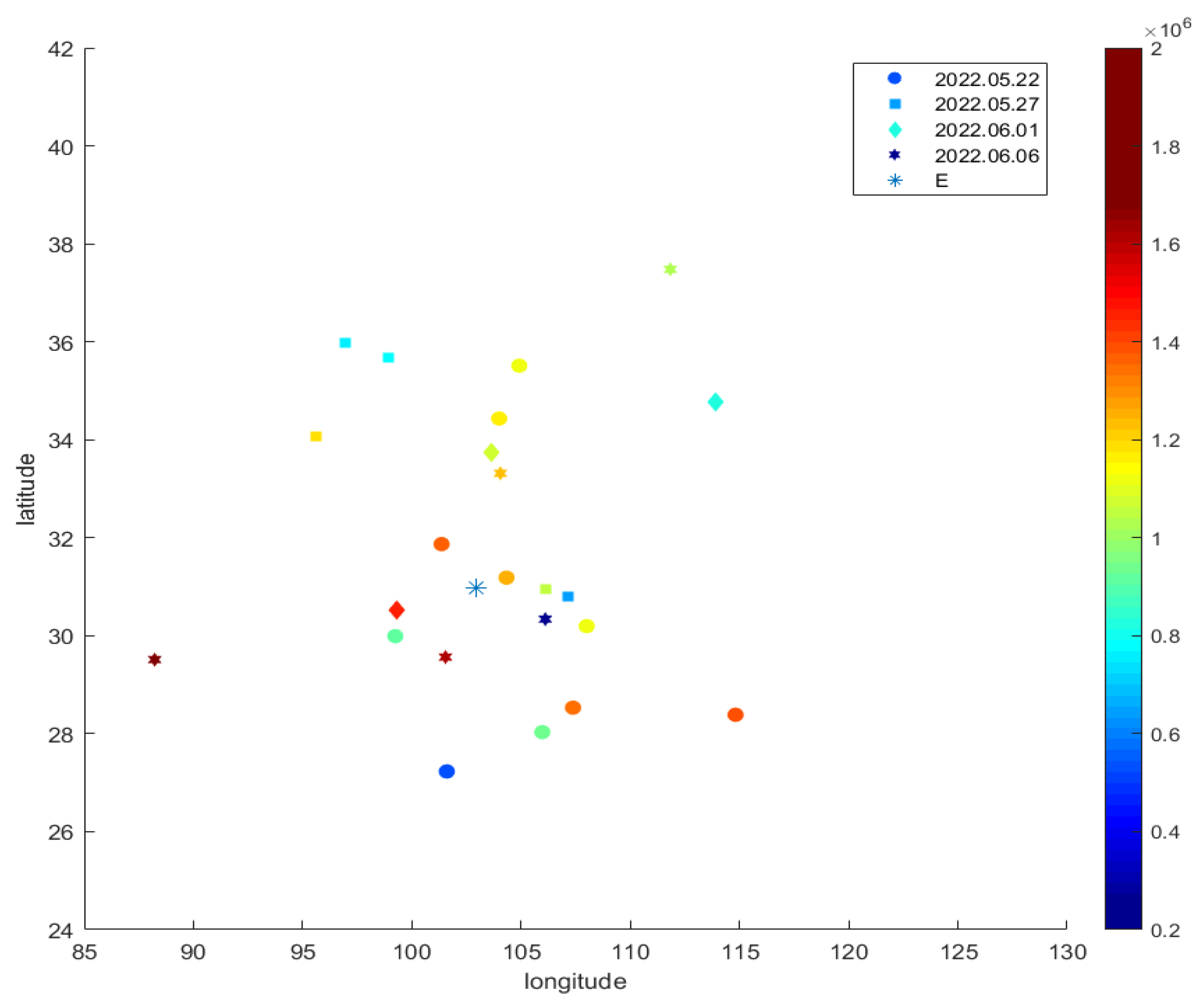
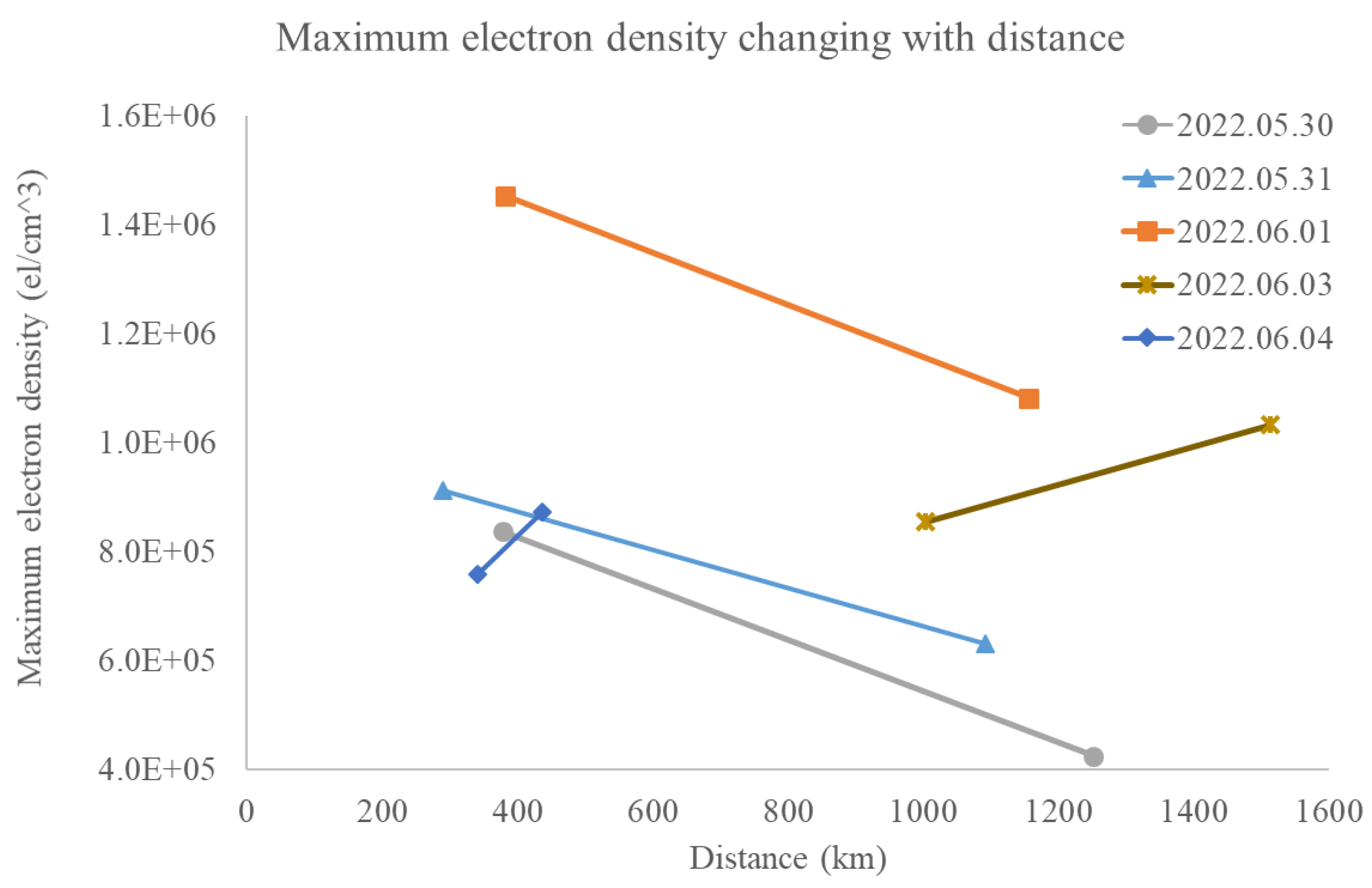
4.2. Change in the Maximum Electron Density

The maximum electron density, marked as the “edmax” index in the data file, is extracted and plotted in Figure 4, distributed in a certain range of 85 degrees to 130 degrees east longitude (E) and 24 degrees to 42 degrees north latitude (N). From 22 May 2022, the maximum electron density distribution in this area, changing at a time interval of 5 days, is illustrated in different symbols representing different dates. The circles represent the data recorded on 22 May 2022, the squares represent the data on 27 May 2022, the diamonds represent the data on 1 June 2022, and the hexagon represents the data on 6 June 2022. The earthquake location is plotted by the asterisk. It can be referred from Figure 4 that the maximum electron density may increase if the measurement location is approaching the earthquake occurrence location, as illustrated by the higher density at a nearby location, “99.27914E, 30.52638N”, on 1 June 2022, and a lower density at a faraway location, “113.90278E, 34.76981N”. Furthermore, the maximum electron density may also increase if the time of measurement is approaching the earthquake occurrence time, as illustrated by the lower density at “99.23926E, 29.99113N” on 22 May 2022 and the higher density at a nearby location, “99.27914E, 30.52638N”, on 1 June 2022. After the earthquake, the maximum electron density may decrease, as illustrated by the very low density at “106.10899E, 30.33856N”.
Generally speaking, an increase in the maximum electron density around the earthquake could be more significant if the occultation measurement time approaches the earthquake occurrence time. In order to validate this intuitive guess, a smaller time interval of the measurements is selected as 3 days, and the collected data are plotted in Figure 5. In Figure 5, the circles represent the data recorded on 26 May 2022, the squares represent the data on 29 May 2022, the diamonds represent the data on 1 June 2022, and the hexagon represents the data on 4 June 2022. The decrease in the maximum electron density after the earthquake can be easily captured by the comparison between the higher density at “99.27914E, 30.52638N” on 1 June 2022 and the lower density at a nearby location, “99.37187E, 30.41836N”, on 4 June 2022.
A more intuitive comparison can be presented by the changing of the maximum electron density curve with the X-axis labeling the distance of the measurement point to the earthquake occurrence location. As shown in Figure 6, the maximum electron density significantly reduces with the increasing distance in all the days before the earthquake, and the highest density can be detected on the day when the earthquake happens at the same distance, as shown in the orange curve with squares. A gradually increasing rule before the earthquake can be figured out from the curves on 30 May 2022 (illustrated in gray circles), 31 May 2022 (illustrated in blue triangles), and 1 June 2022 (illustrated in orange squares). After the earthquake, the density will decrease gradually, as illustrated by the two curves on 3 and 4 June 2022. Furthermore, a sharp decrease can be found on 4 June 2022, which indicates the rapid decrease in the electron density within a certain area nearby after the earthquake happens. In all, the maximum electron density is proved to be an efficient index in the earthquake forecast, and the changing rules in both time and space differences can help us improve the forecast accuracy on the earthquake date and location. A certain area can be determined by the measurement locations, where the maximum electron densities show an obvious increase in a short period.
Based on the point plots illustrating the observations of occultation events, a contour map can be generated to show more clearly the change in the maximum electron density around the earthquake. As shown in Figure 7, the spatial distribution of the maximum electron density from 24 May 2022 to 3 June 2022 is plotted, in which the epicenter is demonstrated by the “*” symbol. The density near the epicenter could be estimated as between 8.5 × 10 5   e l / m 3 and 9.0 × 10 5   e l / m 3 on 24 May 2022, and increased to a larger value between 9.0 × 10 5   e l / m 3 and 1.0 × 10 6   e l / m 3 on 26 May 2022. It further raised up to larger than 1.1 × 10 6   e l / m 3 on 27 May 2022 and 1.3 × 10 6   e l / m 3 on 29 May 2022. The density remains higher than 1.3 × 10 6   e l / m 3 at the epicenter on 1 June 2022, when the earthquake occurred, and sharply decreased to less than 8.0 × 10 6   e l / m 3 on 3 June 2022 after the earthquake. Thus, a clear anomaly of the maximum electron density can be detected five days before the earthquake with a significant increase, starting after 26 May 2022, which gives us more time to prepare for this disaster.
It is also interesting to observe that the peaks in the maximum electron density spatial distribution are located on the south of the epicenter before the earthquake, which is consistent with the findings in [34]. The ionosphere anomaly area is not directly above the epicenter but shifts a certain distance toward the epicenter.

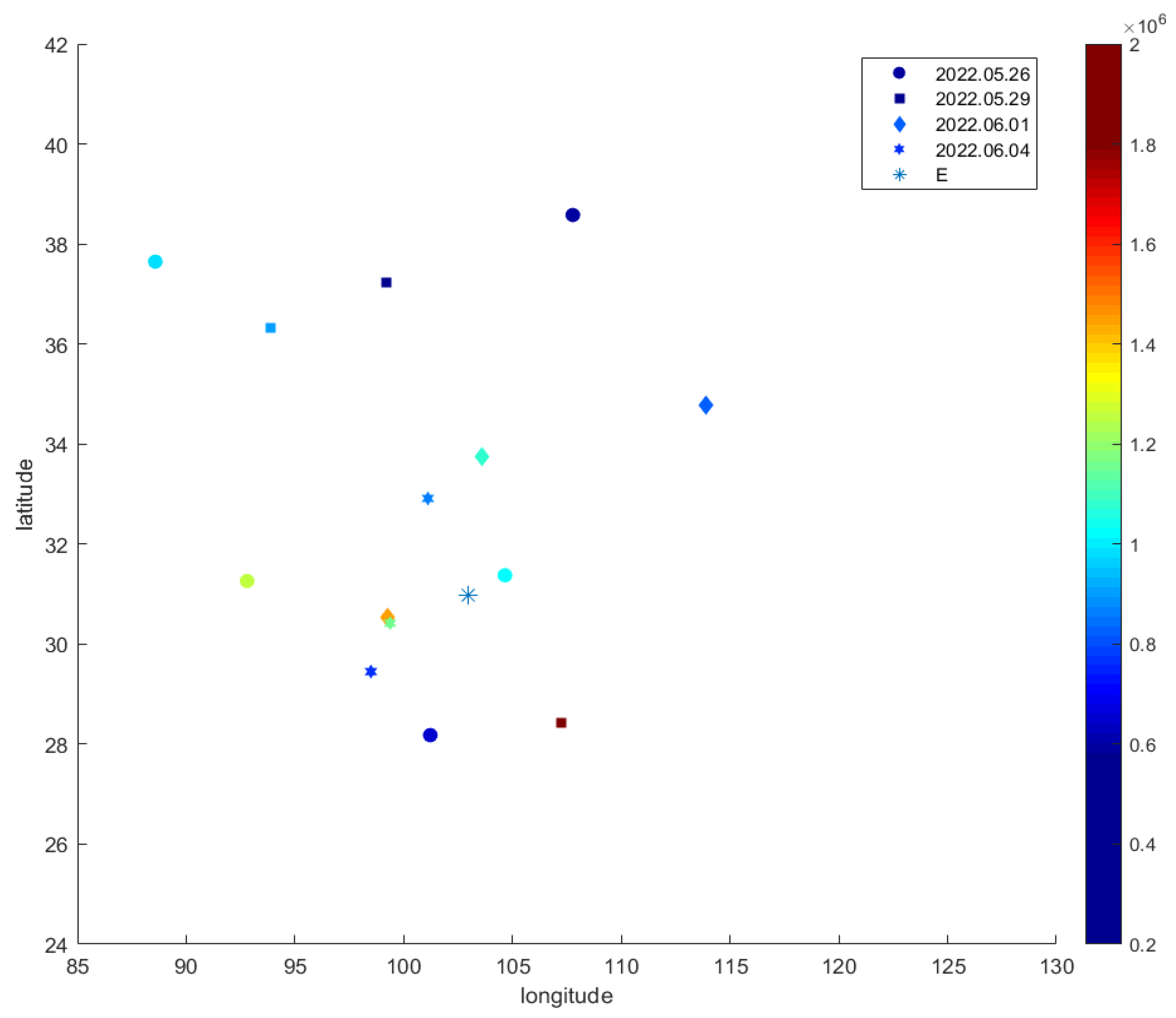
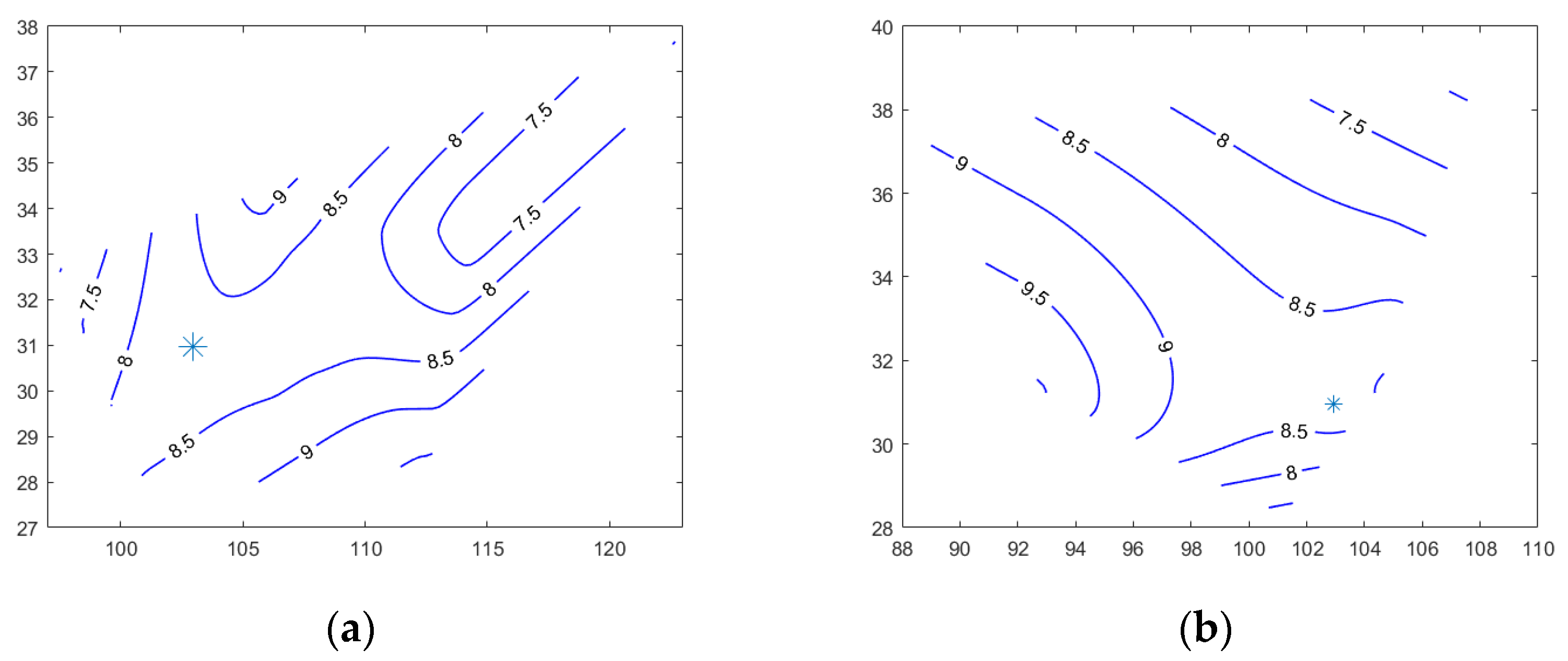
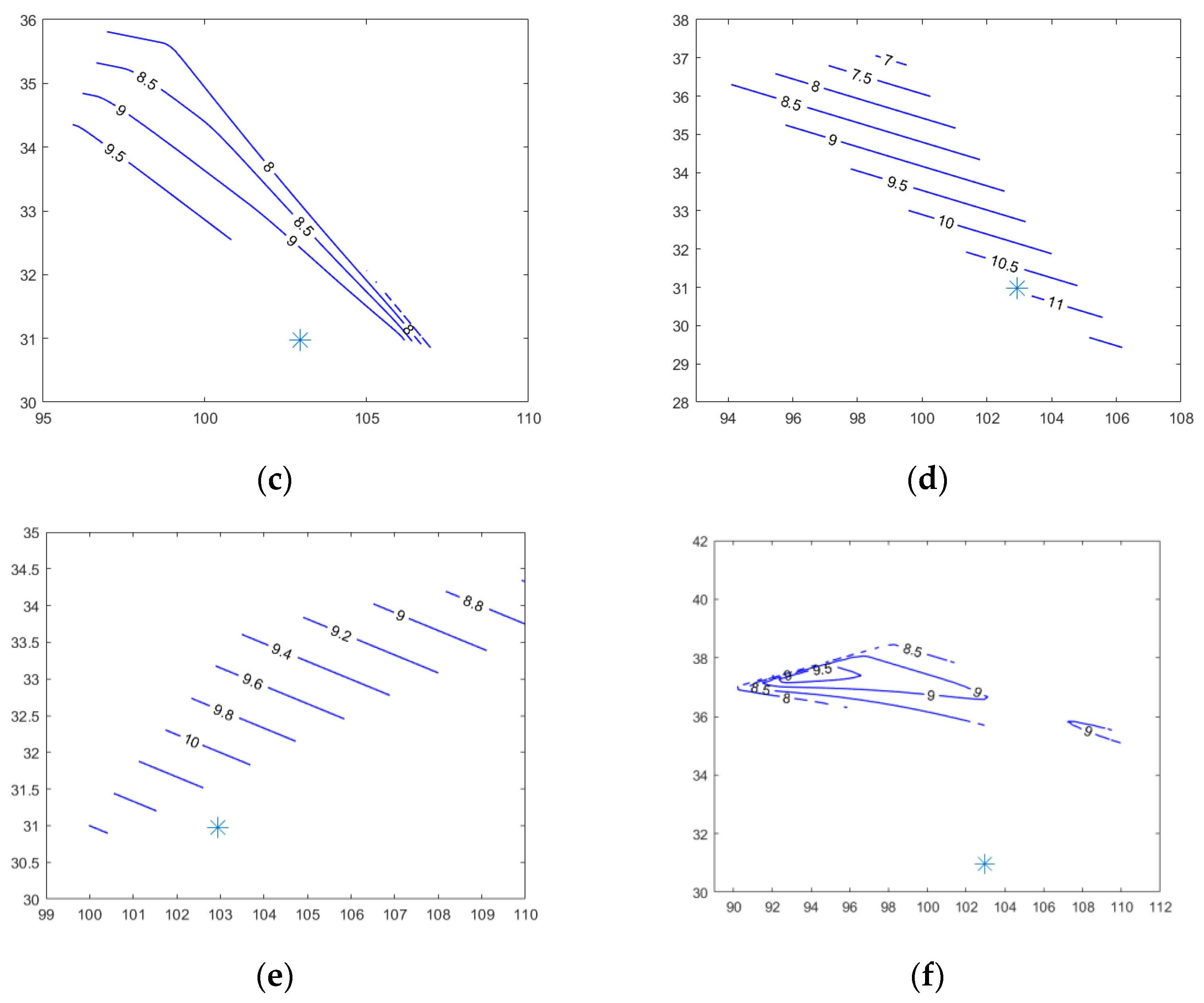
4.3. Change in the Critical Frequency at Maximum Electron Density

Similarly, the critical frequency at maximum electron density, marked as the “critfreq” index in the data file, is extracted and plotted in Figure 8, distributed in a certain range of 85 degrees to 130 degrees east longitude (E) and 24 degrees to 42 degrees north latitude (N). From 26 May 2022, the azimuth angle distribution in this area, changing at a time interval of 1 day, is illustrated in different symbols representing the data on different dates. The changing rule can also be captured as the increase in the azimuth angle with the time approaching the earthquake occurrence. For example, the angle is larger on 31 May 2022 at “100.74227E, 25.61618N”, illustrated by the dark red square, while a smaller angle was measured on 28 May 2022 at a nearby location, “100.37244E, 25.85185N”, illustrated by the blue upwards triangle. Furthermore, a smaller angle can be detected on 27 May 2022 at “107.17728E, 30.79741N”, illustrated by the blue leftwards triangle, while a larger angle can be detected at the same time at a location closer to the earthquake location, illustrated by the green leftwards triangle at “106.1255E, 30.94742N”. Thus, it is further validated that there remain certain space and time rules relevant to the earthquake occurrence, which can be referred from the change in the azimuth angle of the occultation plane with respect to the north at maximum electron density within a certain area and during a certain period.
The time-marching special distribution of the critical frequency at maximum electron density can also be plotted to explain the trend more clearly. As shown in Figure 9, the contour map of the frequency is generated from 24 May 2022 to 3 June 2022, in which the epicenter is demonstrated by the “*” symbol. The frequency near the epicenter can be referred to as between 8 and 8.5 on 24 May 2022, and then increased to between 8.5 and 9.0 on 26 May 2022. A larger frequency was observed on 27 May 2022 as larger than 9.5, and even higher on 29 May 2022 as 11. The frequency kept near 11 on 1 June 2022, and then decreased to less than 8.0 on 3 June 2022. Again, a clear anomaly of the critical frequency can be detected five days before the earthquake with a significant increase, starting after 26 May 2022, which gives us more time to prepare for this disaster.

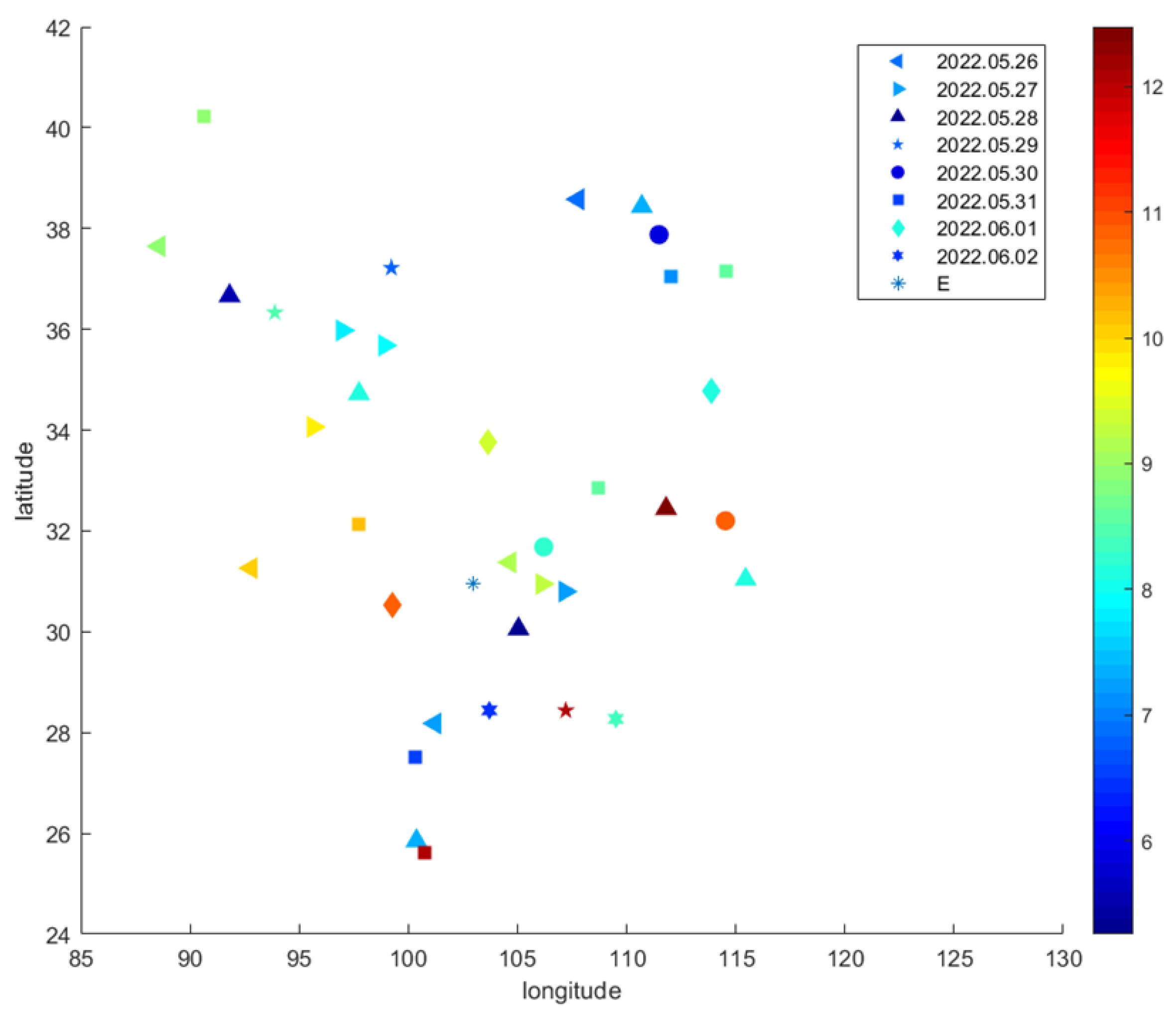
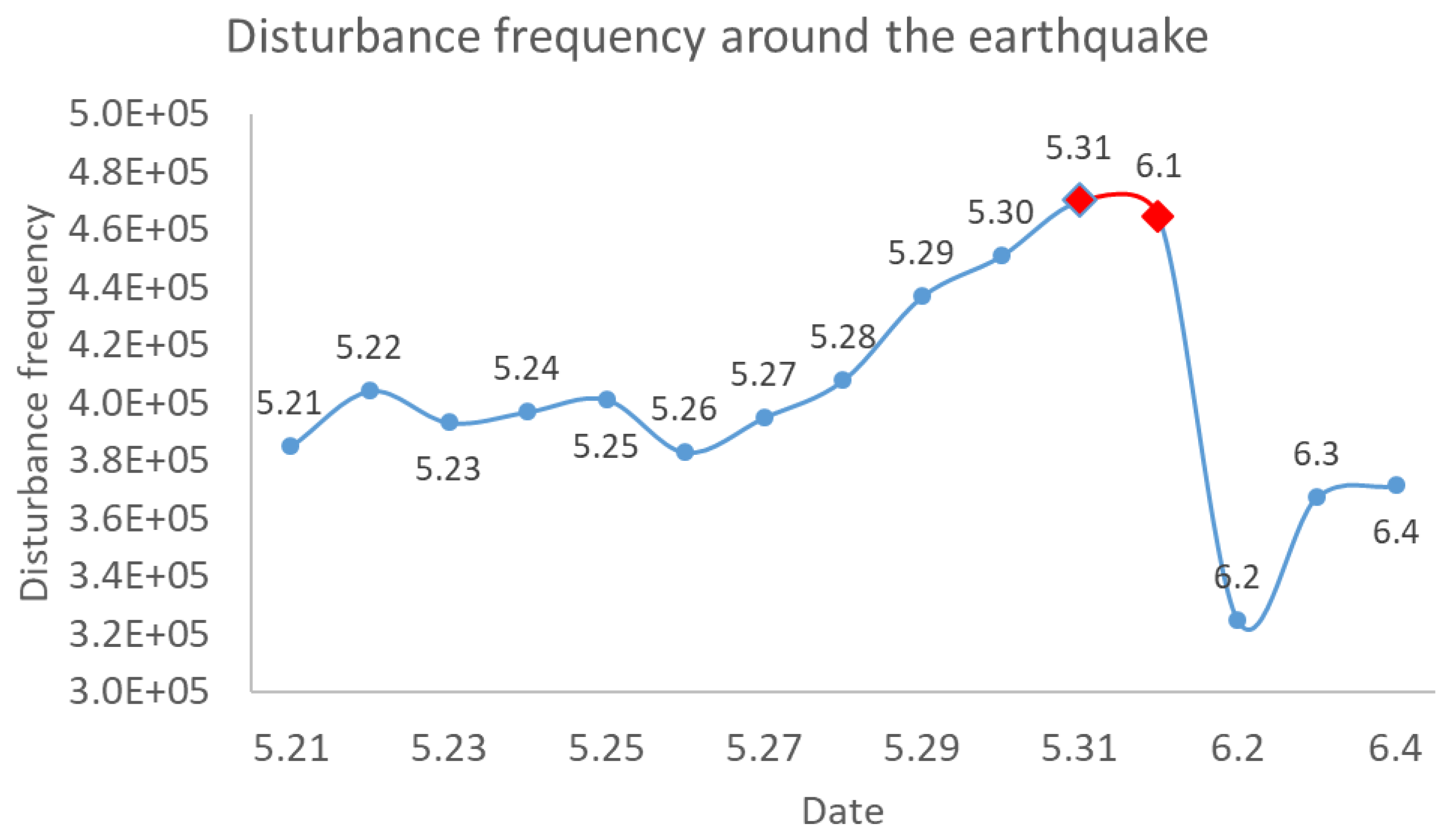
4.4. The Disturbance Frequency

Based on the above analysis, both the maximum electron density and the critical frequency can play a role in forecasting a strong earthquake. However, a quantitative index is more preferred to indicate more directly the time and location of an upcoming earthquake. In particular, the spatial concentration around the epicenter should be considered in the index, but the occultation data cannot ensure an ideal distribution of observation locations due to current technique limitations. In [19], the authors divided the entire region into four sub-regions, and then took the average of each region in the occultation events to introduce the influence of spatial distribution on the ionospheric indexes in the vicinity of the epicenter. However, an average in the subdomain still suffers from spatial homogeneity, which challenges a reliable index. Moreover, not all the observations obey a clear and uniform changing rule. For example, the large density at “114.8183E, 28.38687N” on 22 May 2022 seems strange in Figure 4 as it is far away from the epicenter. Such observations may result from special geomagnetic and electrodynamic environments that disturb the electron distribution other than the earthquake. Thus, other parameters should be involved in formulating the quantitative index, which can involve spatial heterogeneity and reduce the effect of other abnormal disturbances.
In addition, solar activity can also lead to a deviation from the normal state of the ionosphere. The solar chromosphere emits strong ultraviolet and X-ray radiation during the flare eruption, which makes the electron density suddenly increase. A geomagnetic storm is an important geophysical phenomenon with strong geomagnetic field disturbance. Its energy mainly comes from the sun. The plasma cloud emitted from the solar surface propagates through interplanetary space to the top of the earth’s magnetosphere and acts with the earth’s magnetic field to cause geomagnetic storms, leading to global ionospheric changes. The ionospheric changes caused by these effects are global, but the ionospheric disturbances that may be related to earthquakes have obvious localization characteristics. It can be seen from the analysis in the previous section that the closer to the epicenter, the more obvious the ionospheric disturbance is represented by the electron density. Therefore, the influence of spatial distribution should be introduced in the construction of an earthquake forecasting index based on ionospheric disturbance to eliminate the interference of solar activity and geomagnetic storms.
From the occultation inverse algorithms described in Section 2, the total electron content, denoted by “ t e c 0 ” in the data file, may have the potential to balance the spatial heterogeneity and abnormal fluctuations in the maximum electron density. In order to validate this guess, the correlation between “ e d m a x ” and “ t e c 0 ” is analyzed. A strong linear correlation can be observed directly by calculating the correlation coefficient, as shown in Table 2. A large correlation coefficient of 0.9598 validates the effectiveness of balancing “ e d m a x ” using “ t e c 0 ”. The coefficient’s upper bound, 0.9694, and the lower bound, 0.9472, both indicate the strong reliability of this connection. In fact, the maximum electron density in the layer is the main source of the TEC, so the high correlation coefficient between the two data is inevitable.
Thus, a disturbance frequency can be constructed as follows to act as an index forecasting the occurrence of an earthquake:
F = e d m a x × c r i t f r e q t e c 0 ,
where F denotes the disturbance frequency, e d m a x is the maximum electron density in the occultation data, c r i t f r e q is the critical frequency, and t e c 0 is the total electron content. The close correlations among the earthquake occurrence, the maximum electron density, and the critical frequency are shown in Section 4.2 and Section 4.3, with a theoretical mechanism analysis in Section 3, while the denominator t e c 0 is involved to eliminate the effect of observation locations that may affect the index. It should be noted that if more than one observation point is located within the affected area around the epicenter, F should be averaged. As the effect of spatial heterogeneity is reduced, such an average approach is more stable and reliable.
The effectiveness of the proposed disturbance frequency can be validated by showing the changing frequency around the Ya’an earthquake. As shown in Figure 10, a clear positive correlation between the disturbance frequency and earthquake occurrence can be observed. After obtaining the relevant data, only 0.52S is needed to calculate the index in each day using a workstation (Intel(R) Xeon(R) Gold 6230 CPU, 2 × 2.10 GHz, 256 G RAM). From 21 May 2022 to 26 May 2022, the averaged frequency within the affected area remains flat. Starting from 27 May 2022, a significant increase is detected until the observation on 31 May 2022. The frequency remains almost the same for observations in the two days closely around the earthquake, namely 31 May 2022 and 1 June 2022, as plotted by the red curve. Afterwards, a rapid decrease can be detected on 2 June 2022, and then the frequency increases back to the normal value similar to the steady state before 26 May 2022. Thus, at least five days, namely 27–31 May 2022, can be used to make preparations if the abnormal increase in the frequency is detected on time.
In practice, for a monitoring point in an earthquake zone, the averaged disturbance frequency within a certain affecting area should be measured and calculated every day to monitor the abnormal increase. If an increase is detected, we may further change the size of the affected range and test the nearby monitoring point to figure out a more accurate forecast of the location of the epicenter. Moreover, using the Dobrovolsky formula, the earthquake magnitude can also be estimated if the affecting area is determined after a number of trials. As pre-earthquake ionospheric anomalies are generally obvious for strong earthquakes, a significant change in the disturbance frequency may also forecast the occurrence of an upcoming strong earthquake (generally with M ≥ 5.5). Thus, more serious preparations should be conducted to reduce the damage caused by such a disaster.

5. Concluding Remarks

In this paper, we investigate the algorithm of radio occultation and investigate the possible index in the measurement data that may help forecast the occurrence time and location of earthquakes. It has been found that the maximum electron density measured by radio occultation can be used as an effective index indicating the potential time and location range of an earthquake and may also indicate the occurrence of a strong earthquake (M ≥ 5.5). In particular, a larger density is expected if the measurement takes place near the time and location of the earthquake occurrence. A constant increase in density within a certain area is a symbol of a coming earthquake in this area, and the density will sharply decrease after the earthquake as the disturbance ends. Similarly, the critical frequency at maximum electron density is also another index that can help forecast an upcoming earthquake. In particular, a larger frequency is observed near the time and location of the earthquake occurrence. In order to generate a quantitative index forecasting earthquakes, based on the analysis of earthquake occurrence affecting electron density, a disturbance frequency is formulated to calculate an index that may help forecast upcoming earthquakes. As referred from the index performance, occultation data can forecast the occurrence of earthquakes five days ahead of detection. Moreover, the regional scale derived using the Dobrovolsky formula is a good choice to determine the data collection and analysis area.
This paper proposes a new method that might be helpful in earthquake forecasting. There still remains certain work in the accurate forecasting of earthquake occurrence, in terms of the time, location, and magnitude, using this index. For example, in future studies, we may find a general quantitative correlation between the increasing rate of this index and the remaining time to the earthquake occurrence. Using this rule, a more reliable and informative earthquake forecast can be expected. The index formulation can also be validated and maybe optimized if tested in more earthquake circumstances. Investigations of the index performance on the occasion of an earthquake that is not large in magnitude (such as 4 or 5) are also expected in future studies, to give more clear and reliable criteria of the earthquake magnitude that can be forecasted using this index. In other words, magnitude can be included in the index to give a more informative forecast of an earthquake. Studies on after-earthquake ionosphere phenomena can also be promoted, as the mechanisms causing the ionospheric dissipation may be different from those resulting in the ionospheric disturbance before the earthquake. In particular, uplifts have also been detected after earthquakes [50], although sometimes, this is believed to be a consequence of aftershocks.
All the above future developments can only be achievable with much more occultation data, which poses further challenges to data processing, in addition to satellite development. The big data technique and deep learning algorithm may be applied in future studies to process the large amount of data that may be obtained. Moreover, the correlation between earthquake occurrence and the index has been validated, and a deep learning model [51] is expected to be trained to give a fast and reliable prediction of the time, location, and magnitude of an earthquake based on the disturbance index. Advanced data mining techniques [52] can also help identify possible indexes in occultation data that can be included in the index formulation.

Author Contributions

Conceptualization, T.Z. and H.S.; methodology, H.S. and W.B.; software, T.Z.; validation, Y.S. and G.T.; formal analysis, Y.W.; investigation, T.Z. and H.S.; resources, W.B.; data curation, G.T. and X.L.; writing—original draft preparation, T.Z.; writing—review and editing, H.S. and S.S.; visualization, T.Z.; supervision, S.S.; project administration, H.S. and S.S.; funding acquisition, W.B., H.S. and S.S. All authors have read and agreed to the published version of the manuscript.

Funding

This research was funded by the National Natural Science Foundation of China (51936001, 42074042, and 42104032), the Youth Cross Team Scientific Research Project of the Chinese Academy of Sciences (JCTD-2021-10), and the King Abdullah University of Science and Technology (KAUST) through the grants BAS/1/1351-01 and URF/1/5028-01.

Data Availability Statement

Not applicable.

Acknowledgments

We would like to express appreciation to the colleagues in our research group.

Conflicts of Interest

The authors declare no conflict of interest.

Appendix A. Data Preprocessing

The observation time of the occultation event provided by the ionospheric occultation data belongs to the UTC (Coordinated Universal Time) time system [53], and the data storage form is to first record the start time t 0 of the occultation event, and then record the time step at the i th sampling instant s i , and the actual time t i of each occultation instant in the observation sequence can be calculated by t i = t 0 + s i , The time resolution of the occultation data depends on the sampling frequency of the occultation signal receiver [54]. The higher the sampling frequency of the receiver, the higher the time resolution of the occultation data. At present, there are mainly two kinds of frequency, 1 Hz and 50 Hz, which can complete occultation data sampling in the time interval of 1 s and 0.02 s, respectively [55]. The sampling frequency of the neutral atmosphere occultation data provided by the two occultation missions of COSMIC and FY-3C is 50 Hz; that is, the time resolution is 0.02 s [56]. The sampling frequency of the given ionospheric occultation data is 1 Hz; that is, the time resolution is 1 s.
The spatial position and motion speed of GNSS and LEO satellites provided by the ionospheric occultation data belong to the Earth-Centered Inertial (ECI) coordinate system [57], but the perigee latitude and longitude and altitude of the occultation path we need belong to the Earth-Centered Earth-Fixed (ECEF) coordinate system [58], so we need to convert it to ECEF coordinates after solving the ECI coordinates of the perigee. The conversion can be formulated as:
X Y Z = c o s T s i n T 0 s i n T c o s T 0 0 0 1 x y z ,
where X Y Z and x y z denote the ECEF and ECI coordinates, respectively; and T denotes the rotation angle, which is equivalent to Greenwich sidereal time [59] at the vernal equinox, that is, Greenwich sidereal time corresponding to the observation moment. In order to avoid the possible interference of high-frequency noise in the observation sequence with additional phase delay to the inversion results, we need to filter and smooth the observation sequence before inversion.

Appendix B. Doppler Inverse Algorithm

After the original additional phase delay sequence is smoothed [60,61], the additional Doppler frequency shift sequence can be obtained by derivation with respect to time:
c Δ f i f i = d ϕ i d t ,
where c denotes the speed of light in vacuum; f i is the frequency of L1 ( i = 1 ) and L2 ( i = 2 ) bands, respectively; Δ f i is the additional Doppler frequency shift; and ϕ i is the additional phase delay in the L1 and L2 bands. Since both c and f i will be subtracted in the subsequent numerical scheme, c Δ f i f i can be regarded as a whole in the calculation, and there is no need to solve Δ f i separately.
Afterwards, we need to establish the geometric equations for additional Doppler shifts and impact parameters. We define the signal transmission frequency from the GNSS satellites as f s and the signal reception frequency at the LEO satellites as f r , and the Doppler shifts f d can be calculated by the difference between the above two frequencies as f d = f r f s . According to the Doppler principle, f r and f s are correlated with the signal transmission speed v s and the signal reception speed v r , and such correlation can be formulated as:
f r = f s c v r c v s = f s 1 v r c 1 v s c = f s 1 v r c 1 + v s c 1 v s c 1 + v s c = f s 1 v r c + v s c v r v s c 2 1 v s 2 c 2 ,
The Doppler shifts can be calculated by f d = f r f s = f s c v s v r . It should be noted that the Doppler frequency shift here contains two parts. The first is the frequency shift due to the relative motion of the GNSS satellite and the LEO satellite; that is, even in a vacuum environment, the signal propagates in a straight line, but the distance between the signal transmitter and receiver changes due to the relative motion of the GNSS and LEO satellites, which results in the Doppler effect [62]. The second part is that due to the bending effect of the atmosphere on the signal propagation path, the change in the distance between the transmitter and receiver will be different, thus causing the Doppler effect that is different from the ideal environment. Therefore, we define the Doppler frequency shift generated in the vacuum environment as f d 0 and the shift generated by the actual propagation path of the signal in the atmosphere as f d 1 , and the difference between the two is the additional Doppler frequency shift Δ f , Δ f = f d 1 f d 0 . The two shifts can be calculated using Equation (A6) as:
f d 0 = f c v G · e v L · e ,
f d 1 = f c v G · e G v L · e L ,
where v G and v L are the projection vectors of the operating speed of the GNSS satellite and the LEO satellite on the occultation plane, respectively. e is the direction vector of the signal propagation path in the vacuum environment, that is, the unit vector corresponding to the connection between the GNSS satellite and the LEO satellite. e G and e L are the direction vectors of signal transmission and signal reception, respectively. f is the signal carrier frequency, which is 1575.42 MHz in the L1 band and 1227.60 MHz in the L2 band [63]. It can be seen from the geometric relationship in Figure 2 that e can be calculated by the coordinate of the GNSS and LEO satellites as e = r L r G r L r G , where r L and r G denote the coordinates of the LEO and GNSS satellites, respectively, namely the vectors OL and OG . e G and e L can be calculated using the collision parameters as:
e G = R n 90 ° + θ G r G r G ,   e L = R n 90 ° + θ L r L r L ,
where θ G and θ L denote the LOP and GOQ in Figure 2, which can be calculated by θ G = a r c cos p r G and θ L = a r c cos p r L . p denotes the impact parameter [64], namely the length of OP and OQ in Figure 2. R n θ represents a rotation of θ degrees with the normal vector n of the occultation plane as the rotation axis, and the counterclockwise direction is positive, where the normal vector n can be obtained by the cross product of two vectors r G and r L . Thus, the Doppler frequency shift in the following equation can be formulated as a function of the impact parameter p as:
Δ f = f c h p ,
where the function h combines Equations (A4)–(A6).
Based on that, the impact parameter in the case of straight-line propagation is selected as the initial value and substituted into the scheme to start the iterative calculations of p in Equation (A7):
p 0 = r L r G sin θ r L 2 + r G 2 2 r L r G cos θ ,
where θ is equal to the LOG in Figure 2. In fact, the above Equation (A15) is to calculate the height corresponding to the base LG of the triangle LOG.
According to the geometry in Figure 2, the bend angle α can be calculated as:
α = θ a r c cos p r L a r c cos p r G .
Based on the assumption of spherical symmetry [65] of the atmospheric refractive index, α can be described as:
α p = 2 p p + d l n n x d α 1 x 2 p 2 d x ,
The atmospheric refractive index n x can be calculated using the following equation derived from the Abel integral transformation:
n p = e x p 1 π p + α p x 2 p 2 d x .
According to the Kursinski formula [66], the influence of other parameters in the ionosphere except the electron density can be ignored, so the relationship between the refractive index n and the electron density N e   is formulated as follows:
N e = 1 n 40.3 f 2 ,
where the unit of N e is el/cm3.

Appendix C. TOC Inverse Algorithm

In ionospheric occultation [67,68], the TEC on the signal propagation path is equivalent to the integral of the ionospheric electron density N e along the signal propagation path:
T E C = N e   d s .
Substituting the Kursinski formula, Equation (A12), into the above Equation (A13), we can obtain:
T E C = 1 n 40.3 f 2   d s = f 2 40.3 1 n   d s .
Since in ionospheric occultation, the bending angle of the signal propagation path is generally lower than 0.03°, we can approximate the propagation path as a straight line. Based on this assumption, it can be found that the signal propagation paths of the L1 band and the L2 band are the connection between the GNSS satellite and the LEO satellite. Under the approximate premise of straight-line propagation, the impact parameter p can be calculated directly by Equation (A8). There is a one-to-one correspondence between the impact parameter sequence and the TEC sequence. The two data sequences are sorted in ascending order of the impact parameter, and then the derivative of the TEC with respect to the impact parameter, d T E C , can be obtained as:
d T E C = Δ T E C Δ p .
Using the Abel integration [69], the electron density N e can be calculated as:
N e p = 1 π p + d T E C x x 2 p 2 d x .
It is worth noting that the above two occultation inverse methods are essentially the same, but the Doppler-based occultation inverse algorithm requires higher accuracy of satellite position and velocity. Due to the small bending angle of the signal in the ionospheric occultation, it is easy to produce large errors in the inversion. Therefore, the TEC-based occultation inversion algorithm is generally used in the ionospheric occultation inversion process. This is also the inversion algorithm currently adopted by the official ionospheric occultation products of COSMIC and FY-3C.
In the process of ionospheric occultation inverse calculation, whether it is based on Doppler or TEC algorithm will involve calculating the Abel integral of the following formula, y = p + f x x 2 p 2 d x . For the singularity of the upper limit of integration, since the orbital height of the LEO satellite is generally about 800 km [70], and the electron density is very rare above this height, the corresponding bending angle or d T E C is also close to 0, so we can ignore the effect of higher spaces above the orbital height of the LEO satellite and modify the upper limit of the integration to the geocentric distance r L of the LEO satellite, thereby eliminating the singularity of the upper limit of integration. For the singular point of the lower limit of integration, the most direct way is to use truncation, that is, to take a point p t near the lower limit of integration p as the new lower limit of integration, that is,
y p t   r L f x x 2 p 2 d x .
The above truncation method dealing with the singularity of the lower limit of the integration is simple in calculation and widely accepted in practice, but the problem is that the integration accuracy is damaged as the integration within the p ~ p t interval is directly ignored in the integration process [71]. It should be noted that without considering the change trend of f x , the closer the integral variable x is to p , the smaller the denominator x 2 p 2 of the integral function, and the larger the value of the corresponding integral function. Thus, the integral within the p ~ p t interval accounts for a large proportion of the entire Abel integral, so using p t to truncate the lower-limit singularity of the integral may produce a larger integral error. In order to better solve the problem of the singularity of the lower limit of the integral, f x can be approximated under certain assumptions so as to obtain the analytical calculation result of the above Abel integral. It has been explained in [72] that the function f x can be approximated as a linear change in the range of a very small interval x m i n ,   x m a x .
Generally, the time resolution of the ionospheric occultation data is 1 s, and that of the neutral atmosphere occultation data is 0.02 s [73], which indicates that in an occultation event, the impact parameter corresponding to the adjacent sampling changes very little, so we can directly use the two adjacent occultation moments as the division interval of the Abel integral. In addition, in a complete occultation event, the maximum value of the impact parameter is the geocentric distance of the LEO satellite r L . Therefore, we only need to numerically integrate the observation sequence of occultation data to calculate the Abel integral value. We assume that there are N occultation moments in an occultation event, and each occultation moment corresponds to a signal propagation path. Let p i denote the impact parameter corresponding to the i -th occultation instantaneous signal propagation path. Since the resolution of the occultation data is high enough, the impact parameter tends to change slowly, so p i is very close to p i + 1 , then within the integration interval p i ~ p i + 1 the Abel integration result S i can be expressed as:
S i = p i   p i + 1 f x x 2 p 2 d x       i = 1 , 2 , 3 , , N 1 .
According to the additivity property, the Abel integral for the k -th impact parameter can be calculated as:
p + f x x 2 p 2 d x p r L f x x 2 p 2 d x i = k N 1 S i .
This method of removing the singularity of the lower limit of the integral is essential to divide the ionospheric height interval scanned by the occultation event into several heights according to the sampling frequency and consider the bending angle sequence α p or the total electron content differential sequence d T E C p to vary linearly between adjacent altitude layers, starting from the current inverse altitude and ending with the LEO satellite orbital altitude. The Abel integral is calculated layer by layer and finally summarized. If the thickness of the higher layer is narrower, the physical quantities between layers are closer to a linear rule, the error accumulation in the calculation process is also smaller, and the obtained Abel integral value is more accurate. Based on this, this numerical calculation method of the Abel integral is also vividly called the “onion method” [74]. Compared with the method of directly truncating the lower-limit singularity, a higher calculation accuracy can be expected. Currently, the occultation products officially provided by COSMIC and FY-3C adopt this method.

References

  1. Hocke, K.; Pavelyev, A.G.; Yakovlev, O.I.; Barthes, L.; Jakowski, N. Radio occultation data analysis by the radioholographic method. J. Atmos. Sol. Terr. Phys. 1999, 61, 1169–1177. [Google Scholar] [CrossRef]
  2. Sokolovskiy, S.V. Modeling and inverting radio occultation signals in the moist troposphere. Radio Sci. 2001, 36, 441–458. [Google Scholar] [CrossRef] [Green Version]
  3. Ringer, M.A.; Healy, S.B. Monitoring twenty-first century climate using GPS radio occultation bending angles. Geophys. Res. Lett. 2008, 35, 32462. [Google Scholar] [CrossRef] [Green Version]
  4. Shao, H.; Zou, X.; Hajj, G.A. Test of a non-local excess phase delay operator for GPS radio occultation data assimilation. J. Appl. Remote Sens. 2009, 3, 033508. [Google Scholar] [CrossRef]
  5. Padullés, R.; Cardellach, E.; Wang, K.-N.; Ao, C.O.; Turk, F.J.; de la Torre-Juárez, M. Assessment of global navigation satellite system (GNSS) radio occultation refractivity under heavy precipitation. Atmos. Meas. Tech. 2018, 18, 11697–11708. [Google Scholar] [CrossRef] [Green Version]
  6. Schreiner, W.S.; Weiss, J.P.; Anthes, R.A.; Braun, J.; Chu, V.; Fong, J.; Hunt, D.; Kuo, Y.H.; Meehan, T.; Serafino, W.; et al. COSMIC-2 radio occultation constellation: First results. Geophys. Res. Lett. 2020, 47, e2019GL086841. [Google Scholar] [CrossRef]
  7. Chen, W.; Tenzer, R. Reformulation of Parker–Oldenburg’s method for Earth’s spherical approximation. Geophys. J. Int. 2020, 222, 1046–1073. [Google Scholar] [CrossRef]
  8. Zeng, Z.; Sokolovskiy, S. Effect of sporadic E clouds on GPS radio occultation signals. Geophys. Res. Lett. 2010, 37, 44561. [Google Scholar] [CrossRef]
  9. Cucurull, L.; Derber, J.C.; Purser, R.J. A bending angle forward operator for global positioning system radio occultation measurements. J. Geophys. Res. Atmos. 2013, 118, 14–28. [Google Scholar] [CrossRef]
  10. Healy, S.B. Radio occultation bending angle and impact parameter errors caused by horizontal refractive index gradients in the troposphere: A simulation study. J. Geophys. Res. Atmos. 2001, 106, 11875–11889. [Google Scholar] [CrossRef]
  11. Yue, X.; Schreiner, W.S.; Lin, Y.-C.; Rocken, C.; Kuo, Y.-H.; Zhao, B. Data assimilation retrieval of electron density profiles from radio occultation measurements. J. Geophys. Res. Atmos. 2011, 116, 15980. [Google Scholar] [CrossRef] [Green Version]
  12. Jensen, A.S.; Lohmann, M.S.; Nielsen, A.S.; Von Benzon, H.-H. Geometrical optics phase matching of radio occultation signals. Radio Sci. 2004, 39, 1–8. [Google Scholar] [CrossRef] [Green Version]
  13. Emelianov, N.V.; Irsmambetova, T.R.; Kiseleva, T.P.; Tejfel, V.G.; Vashkovjak, S.N.; Glushkova, E.A.; Kornilov, V.G.; Charitonova, G.A. Photometry and position observations of Saturnian satellites during their mutual eclipses and occultations in 1995 performed at the Observatories in Russia and Kazakhstan. Astron. Astrophys. Suppl. Ser. 1999, 139, 47–56. [Google Scholar] [CrossRef] [Green Version]
  14. Xian-Yi, W.; Yue-Qiang, S.; Wei-Hua, B.; Qi-Fei, D.; Dong-Wei, W.; Di, W.; Qing-Long, Y.; Ying, H. Simulation of Number and Distribution of Compass Occultation Events. Chin. J. Geophys. 2013, 56, 373–381. [Google Scholar] [CrossRef]
  15. Allen, R.M.; Melgar, D. Earthquake early warning: Advances, scientific challenges, and societal needs. Annu. Rev. Earth Planet. Sci. 2019, 47, 361–388. [Google Scholar] [CrossRef] [Green Version]
  16. Kunitsyn, V.; Andreeva, E.; Nesterov, I.; Padokhin, A.; Gribkov, D.; Rekenthaler, D.A. Earthquake Prediction Research Using Radio Tomography of the Ionosphere. In Universe of Scales: From Nanotechnology to Cosmology: Symposium in Honor of Minoru M. Freund; Springer International Publishing: Berlin/Heidelberg, Germany, 2014; pp. 109–132. [Google Scholar]
  17. Cornell, C.A. Engineering seismic risk analysis. Bull. Seismol. Soc. Am. 1968, 58, 1583–1606. [Google Scholar] [CrossRef]
  18. Işık, E.; Sağır, Ç.; Tozlu, Z.; Ustaoğlu, Ü.S. Determination of Urban Earthquake Risk for Kırşehir, Turkey. Earth Sci. Res. J. 2019, 23, 237–247. [Google Scholar] [CrossRef] [Green Version]
  19. Xinxin, M.; Zhan, L.; Huaran, C.; Honglin, J.; Dahu, L.; Liguo, J.; Xiaocan, L. Ionosphere anomaly before the Wenchuan M S 8.0 earthquake detected by COSMIC occultation data. Acta Seismol. Sin. 2013, 35, 848–855. [Google Scholar]
  20. Coburn, A.; Spence, R. Earthquake Protection; John Wiley Sons: Hoboken, NJ, USA, 2002. [Google Scholar]
  21. Liu, J.Y.; Chuo, Y.J.; Shan, S.J.; Tsai, Y.B.; Chen, Y.I.; Pulinets, S.A.; Yu, S.B. Pre-Earthquake Ionospheric Anomalies Registered by Continuous GPS TEC Measurements. In Annales Geophysicae; Copernicus Publications: Göttingen, Germany, 2004; Volume 22, pp. 1585–1593. [Google Scholar]
  22. Silina, A.S.; Liperovskaya, E.V.; Liperovsky, V.A.; Meister, C.-V. Ionospheric phenomena before strong earthquakes. Nat. Hazards Earth Syst. Sci. 2001, 1, 113–118. [Google Scholar] [CrossRef] [Green Version]
  23. Pulinets, S.; Legen’Ka, A.; Gaivoronskaya, T.; Depuev, V. Main phenomenological features of ionospheric precursors of strong earthquakes. J. Atmos. Sol. Terr. Phys. 2003, 65, 1337–1347. [Google Scholar] [CrossRef]
  24. Leonard, R.S.; Barnes Jr, R.A. Observation of ionospheric disturbances following the Alaska earthquake. J. Geophys. Res. 1965, 70, 1250–1253. [Google Scholar] [CrossRef]
  25. Liu, J.Y.; Chen, Y.I.; Chuo, Y.J.; Chen, C.S. A statistical investigation of preearthquake ionospheric anomaly. J. Geophys. Res. Atmos. 2006, 111, 11333. [Google Scholar] [CrossRef] [Green Version]
  26. Cai, J.T.; Zhao, G.Z.; Zhan, Y.; Tang, J.; Chen, X.B. The study on ionospheric disturbances during earthquakes. Prog. Geophys. 2007, 22, 695–701. [Google Scholar]
  27. Calais, E.; Minster, J.B. GPS detection of ionospheric perturbations following the January 17, 1994, Northridge Earthquake. Geophys. Res. Lett. 1995, 22, 1045–1048. [Google Scholar] [CrossRef]
  28. Hauksson, E.; Jones, L.M.; Hutton, K. The 1994 Northridge earthquake sequence in California: Seismological and tectonic aspects. J. Geophys. Res. Solid Earth 1995, 100, 12335–12355. [Google Scholar] [CrossRef]
  29. Le, H.; Liu, J.; Zhao, B.; Liu, L. Recent progress in ionospheric earthquake precursor study in China: A brief review. J. Asian Earth Sci. 2015, 114, 420–430. [Google Scholar] [CrossRef]
  30. Lin, J.; Wu, Y.; Zhu, F.Y.; Qiao, X.; Zhou, Y. Wenchuan earthquake ionosphere TEC anomaly detected by GPS. Chin. J. Geophys. 2009, 52, 297–300. [Google Scholar]
  31. Chuo, Y.J.; Liu, J.Y.; Kamogawa, M. The anomalies in the foEs prior to M ≥ 6.0 Taiwan earthquakes, Seismo Elect romagnetic: Lithosphere Atmosphere Ionosphere coupling. Terrapub 2002, 309–312. [Google Scholar]
  32. Liu, J.-Y.; Tsai, Y.-B.; Chen, C.-H.; Chen, Y.-I.; Yen, H.-Y. Integrated Search for Taiwan Earthquake Precursors (iSTEP). IEEJ Trans. Fundam. Mater. 2016, 136, 214–220. [Google Scholar] [CrossRef]
  33. Pulinets, S. Strong earthquake prediction possibility with the help of topside sounding from satellites. Adv. Space Res. 1998, 21, 455–458. [Google Scholar] [CrossRef]
  34. Pulinets, S.; Boyarchuk, K. Ionospheric Precursors of Earthquakes; Springer Science Business Media: Berlin, Germany, 2004. [Google Scholar]
  35. Liu, L.; Wan, W.; Zhang, M.-L.; Zhao, B. Case Study on Total Electron Content Enhancements at Low Latitudes during Low Geomagnetic Activities before the Storms. In Annales Geophysicae; Copernicus GmbH: Göttingen, Germany, 2008; Volume 26, pp. 893–903. [Google Scholar]
  36. Ding, Z.H.; Wu, J.; Sun, S.J.; Chen, J.S.; Ban, P.P. The variation of ionosphere on some days before the Wenchuan earthquake. Chin. J. Geophys. 2010, 53, 30–38. [Google Scholar]
  37. Parrot, M.; Berthelier, J.J.; Lebreton, J.P.; Sauvaud, J.A.; Santolík, O.; Blecki, J. Examples of unusual ionospheric observations made by the DEMETER satellite over seismic regions. Phys. Chem. Earth Parts A/B/C 2006, 31, 486–495. [Google Scholar] [CrossRef]
  38. Zhao, B.; Wang, M.; Yu, T.; Wan, W.; Lei, J.; Liu, L.; Ning, B. Is an unusual large enhancement of ionospheric electron density linked with the 2008 great Wenchuan earthquake? J. Geophys. Res. Space Phys. 2008, 113, 13613. [Google Scholar] [CrossRef]
  39. Liu, J.Y.; Chen, C.H.; Tsai, H.F.; Le, H. A statistical study on seismo-ionospheric anomalies of the total electron content for the period of 56 M≥ 6.0 earthquakes occurring in China during 1998–2012. Chin. J. Space Sci. 2013, 33, 258–269. [Google Scholar]
  40. Vidale, J.E.; Shearer, P.M. A survey of 71 earthquake bursts across southern California: Exploring the role of pore fluid pressure fluctuations and aseismic slip as drivers. J. Geophys. Res. Atmos. 2006, 111, B05312. [Google Scholar] [CrossRef] [Green Version]
  41. Masci, F.; Thomas, J.N.; Villani, F.; Secan, J.A.; Rivera, N. On the onset of ionospheric precursors 40 min before strong earthquakes. J. Geophys. Res. Space Phys. 2015, 120, 1383–1393. [Google Scholar] [CrossRef]
  42. Hao, Y.; Li, Q.; Guo, J.; Zhang, X.; Yang, G.; Zhang, D.; Xiao, Z. Imaging of the large-scale ionospheric disturbances induced by seismic waves using GPS network in China. Chin. J. Geophys. 2021, 64, 3925–3932. [Google Scholar]
  43. Hayakawa, M.; Molchanov, O.A. Summary report of NASDA’s earthquake remote sensing frontier project. Phys. Chem. Earth Parts A/B/C 2004, 29, 617–625. [Google Scholar] [CrossRef]
  44. Shvets, A.V.; Hayakawa, M.; Maekawa, S. Results of subionospheric radio LF monitoring prior to the Tokachi (m= 8, Hokkaido, 25 September 2003) earthquake. Nat. Hazards Earth Syst. Sci. 2004, 4, 647–653. [Google Scholar] [CrossRef] [Green Version]
  45. Ohta, K.; Izutsu, J.; Schekotov, A.; Hayakawa, M. The ULF/ELF electromagnetic radiation before the 11 March 2011 Japanese earthquake. Radio Sci. 2013, 48, 589–596. [Google Scholar] [CrossRef]
  46. Pulinets, S.A.; Ouzounov, D.; Ciraolo, L.; Singh, R.; Cervone, G.; Leyva, A.; Dunajecka, M.; Kotsarenko, A. Thermal, Atmospheric and Ionospheric Anomalies around the Time of the Colima M7. 8 Earthquake of 21 January 2003. In Annales Geophysicae; Copernicus GmbH: Göttingen, Germany, 2006; Volume 24, pp. 835–849. [Google Scholar]
  47. Zhang, Y.; Liu, X.; Guo, J.; Shi, K.; Zhou, M.; Wang, F. Co-Seismic Ionospheric Disturbance with Alaska Strike-Slip Mw7.9 Earthquake on 23 January 2018 Monitored by GPS. Atmosphere 2021, 12, 83. [Google Scholar] [CrossRef]
  48. Klimenko, M.V.; Klimenko, V.V.; Karpov, I.V.; Zakharenkova, I.E. Simulation of seismo-ionospheric effects initiated by internal gravity waves. Russ. J. Phys. Chem. B 2011, 5, 393–401. [Google Scholar] [CrossRef]
  49. Dobrovolsky, I.P.; Zubkov, S.I.; Miachkin, V.I. Estimation of the size of earthquake preparation zones. Pure Appl. Geophys. 1979, 117, 1025–1044. [Google Scholar] [CrossRef]
  50. Němec, F.; Santolík, O.; Parrot, M.; Berthelier, J.J. Spacecraft observations of electromagnetic perturbations connected with seismic activity. Geophys. Res. Lett. 2008, 35, L05109. [Google Scholar] [CrossRef] [Green Version]
  51. Zhang, T.; Li, Y.; Li, Y.; Sun, S.; Gao, X. A self-adaptive deep learning algorithm for accelerating multi-component flash calculation. Comput. Methods Appl. Mech. Eng. 2020, 369, 113207. [Google Scholar] [CrossRef]
  52. Behrad, F.; Abadeh, M.S. An overview of deep learning methods for multimodal medical data mining. Expert Syst. Appl. 2022, 200, 117006. [Google Scholar] [CrossRef]
  53. Jiang, Z.; Petit, G. Combination of TWSTFT and GNSS for accurate UTC time transfer. Metrologia 2009, 46, 305. [Google Scholar] [CrossRef]
  54. Gorbunov, M.E.; Ao, C.O. Simulation studies of GPS radio occultation measurements. Radio Sci. 2003, 38, 1–5. [Google Scholar]
  55. Steiner, A.K.; Kirchengast, G.; Ladreiter, H.P. Inversion, Error Analysis, and Validation of GPS/MET Occultation Data. In Annales Geophysicae; Springer: Berlin, Germany, 1998; Volume 17, pp. 122–138. [Google Scholar]
  56. Xu, X.; Luo, J.; Wang, H.; Liu, H.; Hu, T. Morphology of sporadic E layers derived from Fengyun-3C GPS radio occultation measurements. Earth Planets Space 2022, 74, 55. [Google Scholar] [CrossRef]
  57. Hasan, M.Z.; Yaacob, S.; Ahmed, A.; Hamzah, N.H.; Yaakob, S.B.; Idris, M.H.; Said, A. Analysis on attitude position of earth centered inertial (ECI) based on razaksat data. J. Teknol. 2015, 76, 5887. [Google Scholar] [CrossRef] [Green Version]
  58. Zhu, J. Conversion of Earth-centered Earth-fixed coordinates to geodetic coordinates. IEEE Trans. Aerosp. Electron. Syst. 1994, 30, 957–961. [Google Scholar] [CrossRef]
  59. Capitaine, N.; Gontier, A.M. Accurate procedure for deriving UTI at a submilliarcsecond accuracy from Greenwich Sidereal Time or from the stellar angle. Astron. Astrophys. 1993, 275, 645. [Google Scholar]
  60. Amar, A.; Weiss, A.J. Localization of Narrowband Radio Emitters Based on Doppler Frequency Shifts. IEEE Trans. Signal Process 2008, 56, 5500–5508. [Google Scholar] [CrossRef]
  61. Schreiner, W.S.; Sokolovskiy, S.V.; Rocken, C.; Hunt, D.C. Analysis and validation of GPS/MET radio occultation data in the ionosphere. Radio Sci. 1999, 34, 949–966. [Google Scholar] [CrossRef]
  62. Seddon, N.; Bearpark, T. Observation of the Inverse Doppler Effect. Science 2003, 302, 1537–1540. [Google Scholar] [CrossRef]
  63. Emara, M.K.; Hautcoeur, J.; Panther, G.; Wight, J.S.; Gupta, S. Surface Impedance Engineered Low-Profile Dual-Band Grooved-Dielectric Choke Ring for GNSS Applications. IEEE Trans. Antennas Propag. 2019, 67, 2008–2011. [Google Scholar] [CrossRef]
  64. Petricca, F.; Cascioli, G.; Genova, A. A Technique for the Analysis of Radio Occultation Data to Retrieve Atmospheric Properties and Associated Uncertainties. Radio Sci. 2021, 56, 1–18. [Google Scholar] [CrossRef]
  65. Claret, A. A new method to compute limb-darkening coefficients for stellar atmosphere models with spherical symmetry: The space missions TESS, Kepler, CoRoT, and MOST. Astron. Astrophys. 2018, 618, A20. [Google Scholar] [CrossRef] [Green Version]
  66. Mannucci, A.J.; Ao, C.O.; Iijima, B.A.; Meehan, T.K.; Vergados, P.; Kursinski, E.R.; Schreiner, W.S. An assessment of reprocessed GPS/MET observations spanning 1995–1997. Atmos. Meas. Tech. 2021, 15, 4971–4987. [Google Scholar] [CrossRef]
  67. Forootan, E.; Kosary, M.; Farzaneh, S.; Kodikara, T.; Vielberg, K.; Fernandez-Gomez, I.; Borries, C.; Schumacher, M. Forecasting global and multi-level thermospheric neutral density and ionospheric electron content by tuning models against satellite-based accelerometer measurements. Sci. Rep. 2022, 12, 2095. [Google Scholar] [CrossRef]
  68. Okoh, D.; Habarulema, J.B.; Rabiu, B.; Seemala, G.; Wisdom, J.B.; Olwendo, J.; Obrou, O.; Matamba, T.M. Storm-time modeling of the African regional ionospheric total electron content using artificial neural networks. Space Weather. 2020, 18, e2020SW002525. [Google Scholar] [CrossRef]
  69. Cheng, Y.; Lin, J.; Shen, X.; Wan, X.; Li, X.; Wang, W. Analysis of GNSS radio occultation data from satellite ZH-01. Earth Planet. Phys. 2018, 2, 499–504. [Google Scholar] [CrossRef]
  70. Polat, H.C.; Tekinalp, O. Solar Sail Application with a Proposed Low Earth Orbit Mission Concept. In Proceedings of the 2019 9th International Conference on Recent Advances in Space Technologies (RAST) IEEE, Istanbul, Turkey, 11–14 June 2019; pp. 285–291. [Google Scholar]
  71. Adhikari, L.; Ho, S.-P.; Zhou, X. Inverting COSMIC-2 Phase Data to Bending Angle and Refractivity Profiles Using the Full Spectrum Inversion Method. Remote Sens. 2021, 13, 1793. [Google Scholar] [CrossRef]
  72. Peng, G.; Haojian, Y.; Zhenjie, H.; Min, L.; Cheng, H. On the singular point of Abel integral transformation in GPS/LEO occultation technology. Acta Astrono. Sin. 2004, 45, 330–336. [Google Scholar]
  73. Schreiner, W.; Rocken, C.; Sokolovskiy, S.; Hunt, D. Quality assessment of COSMIC/FORMOSAT-3 GPS radio occultation data derived from single-and double-difference atmospheric excess phase processing. GPS Solut. 2010, 14, 13–22. [Google Scholar] [CrossRef]
  74. Daun, K.J.; Thomson, K.A.; Liu, F.; Smallwood, G. Deconvolution of axisymmetric flame properties using Tikhonov regularization. Appl. Opt. 2006, 45, 4638–4646. [Google Scholar] [CrossRef]
Figure 1. Schematic diagram of the radio occultation measurements.
Remotesensing 15 03089 g001
Figure 2. Schematic diagram of the instantaneous geometric relationship of occultation.
Remotesensing 15 03089 g002
Figure 3. Schematic diagram of hypothesis of seismo-ionospheric disturbance mechanisms.
Remotesensing 15 03089 g003
Figure 4. Changing of the maximum electron density distribution at intervals of 5 days.
Remotesensing 15 03089 g004
Figure 5. Changing of the maximum electron density distribution at intervals of 3 days.
Remotesensing 15 03089 g005
Figure 6. Changing of the maximum electron density around the earthquake.
Remotesensing 15 03089 g006
Figure 7. Change in the maximum electron density spatial distribution around the earthquake. (a) 24 May 2022; (b) 26 May 2022; (c) 27 May 2022; (d) 29 May 2022; (e) 1 June 2022; (f) 3 June 2022. The “*” symbol denotes the epicenter.
Remotesensing 15 03089 g007
Figure 8. Changing of the critical frequency at maximum electron density at intervals of 1 day.
Remotesensing 15 03089 g008
Figure 9. Change in the critical frequency spatial distribution around the earthquake. (a) 24 May 2022; (b) 26 May 2022; (c) 27 May 2022; (d) 29 May 2022; (e) 1 June 2022; (f) 3 June 2022; * denotes the epicenter.
Remotesensing 15 03089 g009aRemotesensing 15 03089 g009b
Figure 10. Changing of the critical frequency at maximum electron density at intervals of 1 day. The red points and curve denote the period, during which the earthquake occurred.
Remotesensing 15 03089 g010
Table 1. The statistical information of the two key indexes.
Index Mean MinimumMaximum Median Standard
Deviation
Maximum electron density 9.7 × 10 5 2.5 × 10 5 2.7 × 10 6 8.4 × 10 5 4.5 × 10 5
Critical frequency8.64.514.78.22.0
Table 2. Correlation coefficient between edmax and tec0.
CoefficientRRLRU
Value 0.95980.94730.9694
Disclaimer/Publisher’s Note: The statements, opinions and data contained in all publications are solely those of the individual author(s) and contributor(s) and not of MDPI and/or the editor(s). MDPI and/or the editor(s) disclaim responsibility for any injury to people or property resulting from any ideas, methods, instructions or products referred to in the content.

