Inverse Scattering Series Internal Multiple Attenuation in the Common-Midpoint Domain

Abstract

Internal multiple prediction remains a high-priority problem in seismic data processing, such as subsurface imaging and quantitative amplitude analysis and inversion, particularly in the common-midpoint (CMP) gathers, which contain multicoverage reflection information of the subsurface. Internal multiples, generated by unknown reflectors in complex environments, can be reconstructed with certain combinations of seismic reflection events using the inverse scattering series internal multiple prediction algorithm, which is usually applied to shot records in source–receiver coordinates. The computational overhead is one of the major challenges limiting the strength of the multidimensional implementation of the prediction algorithm, even in the coupled plane-wave domain. In this paper, we first comprehensively review the plane-wave domain inverse scattering series internal multiple prediction algorithm, and we propose a new scheme of achieving 2D multiple attenuation using a 1.5D prediction algorithm in the CMP domain, which significantly reduces the computational burden. Moreover, we quantify the difference in behavior of the 1.5D prediction algorithm for the shot/receiver and the CMP gathers on tilted strata. Numerical analysis of prediction errors shows that the 1.5D algorithm is more capable of handling dipping generators in the CMP domain than in the shot/receiver gathers, and it is able to predict the accredited traveltimes of internal multiples caused by dipping reflectors with small inclinations. For more complex cases with large inclination, using the 1.5D prediction algorithm, internal multiple predictions fail both in the CMP domain and in the shot/receiver gathers, which require the full 2D prediction algorithm. To attenuate internal multiples in the CMP gathers generated by large-dipping strata, a modified version is proposed based on the full 2D plane-wave domain internal multiple prediction algorithm. The results show that the traveltimes of internal multiples caused by dipping generators seen in the simple benchmark example are correctly predicted in the CMP domain using the modified 2D prediction algorithm.

1. Introduction

One of the main objectives of reflection seismic is to derive an image of the subsurface from multifold coverage reflection seismic data. To enhance quality and resolution, the source–receiver coordinated seismic records are usually sorted into the common-midpoint (CMP) gathers because of the redundancy source–receiver pairs share. Multiple attenuation in the CMP domain is still a key component, as their occurrence may mislead reflector relocating in migration and destroy seismic quantitative amplitude analysis and interpretation [1,2]. Most of the multiple attenuation methods presented in the CMP domain are based on their periodicity or the difference of velocity stacking between multiples and primaries, such as predictive deconvolution, Radon transform [3,4,5] and velocity stacking [6,7,8], which works at near- or far-offsets, respectively, for surface-related or layer-interbed multiples. In addition, Ref. [9] proposed a modification of the inverse data space method, which was first introduced by [10], for internal multiple attenuation in the CMP gathers with dramatically reduced computational overhead in comparison with the shot gathers. However, internal multiple attenuation in the inverse data space requires an explicit subsurface velocity model, which is not applicable for some cases. Therefore, in complex land data, internal multiple prediction encounters significant challenges due to the lack of periodicity and unambiguous velocity discrimination.

Recently, the Marchenko-based internal multiple attenuation methods have attracted much attention and have achieved some success in some complex cases [11,12,13,14,15]. However, different sets of features or prior knowledge are required by various Marchenko-based approaches. For examples, the Marchenko-based multiple elimination approach proposed by [14] requires a smooth subsurface velocity model and a re-datuming process of source and receivers. The approach introduced by [16] involves defining a virtual multiple generator that needs to reside under a known, well-positioned reflector. Detailed features and assumptions required by various Marchenko-based multiple attenuation approaches can be found in [17].

In addition to the Marchenko portfolio, Refs. [18,19] indicated that, with the inverse scattering series scheme, internal multiples can be reconstructed by combining reflection events satisfying a lower–higher–lower relationship in pseudo-depth with no subsurface information required, whose predictions are usually achieved using shot records in source–receiver coordinates. Many features and difficulties need to be addressed for successfully proceeding internal multiple predictions in complex environments, even through this full data-driven method [20]. Refs. [21,22] proposed modifications to address the approximate nature of the predicted amplitudes, which were first discussed by [23]. In addition, ref. [24] proposed an extended prediction algorithm to enhance the fidelity of the predicted amplitude and phase by accommodating the source wavelet.

Another key component of implementing the inverse scattering series internal multiple prediction practically is the selection of the searching parameter $ϵ$, which limits the proximity of events combined to generate the prediction and increases the computational complexity of its full multidimensional implementation. Ref. [25] introduced the 1.5D time- and offset-time domain versions of the algorithm, which allows a non-stationary $ϵ$ and can be properly extended to 2D and 3D with a plane-wave formulation. Some key positive characteristics, the relative stationarity of optimum parameter and less computational costs, are found in implementation of the algorithm in the coupled plane-wave domain [26]. Moreover, by taking advantage of the plane-wave domain formulation, ref. [27] also reformulated the elastic multicomponent prediction algorithm into the plane-wave domain and introduced an analytically determined vertical traveltime stretching formula to accommodate disordering reflecting interfaces caused by the wave-mode conversion in elastic cases.

Researchers have made positive progress in the inverse scattering series prediction algorithm; however, implementations are all performed in the domain of source–receiver coordinates with the common shot/receiver records. In this paper, we proposed a modification of the algorithm, which has the same characteristics of the pristine formula, to accommodate the CMP domain input. Considering the expensive computational overhead of its multidimensional implementation, for some cases, internal multiples may be predicted using the 1.5D prediction algorithm with acceptable tolerances of the prediction errors [28]. The numerical simulated examples allow us to exemplify the error analysis of implementing the 1.5D prediction algorithm on tilted strata and examine the differences in internal multiple prediction in the CMP gathers and shot/receiver records.

2. Plane-Wave Domain Inverse Scattering Series Internal Multiple Prediction Algorithm (2D): Review

Refs. [18,19] first demonstrated that, with the knowledge of the source signature, internal multiples can be predicted by summing over triplets of events whose pseudo-depths satisfy a lower–higher–lower relationship, wherein the phases of the lower (or deeper) two events are added and the phase of the higher (or shallower) event is subtracted. The algorithm was initially proposed in the wavenumber/pseudo-depth $(k_g,k_s,\tilde{z})$ domain. Considering the adjacent relationship of wavenumber and horizontal slowness $(k=\omega p)$, refs. [26,29] showed the prediction algorithm based on the inverse scattering series can be rewritten in the horizontal-slowness/pseudo-depth $(p_g,p_s,\tilde{z})$. Ref. [26] initially performed internal multiple predictions in the coupled plane-wave domain $(p_g,p_s,\tau )$ and summarized significant advantages of the plane-wave domain algorithm, such as much more sparse inputs, less computational overhead, and a relatively stationary searching parameter.

One of the key obstacles of implementing the inverse scattering series internal multiple prediction algorithm is the selection of the searching parameter $ϵ$, especially in the vanilla domain, i.e., wavenumber/pseudo-depth $(k_g,k_s,\tilde{z})$ domain, due to the energy of input $b_1(k_g,k_s,\tilde{z})$ being significantly spread out with increasing wavenumbers [25,26], which results in a non-stationary searching parameter. However, ref. [26] indicated that the input $b_1(p_g,p_s,\tau )$ in the plane-wave domain allows a stationary searching parameter while perserving the lower–higher–lower relationship. The value of the fixed optimal searching parameter in the plane-wave domain is determined by the width of the wavelet. Detailed comparions of implementing inverse scattering series internal multiple prediction algorithms in variant domains can be found in [26]. Considering these advantages of predictions using the plane-wave transformation, all implementations of internal multiple attenuation will be carried out in the plane-wave domain in this paper.

Let $d(x_g,x_s,t)$ represent a fully deghosted 2D seismic data set involving waves downgoing from the source and upgoing to the receiver, with $x_g$ being the inline receiver coordinate, $x_s$ being the inline source coordinate, and t being the two-way traveltime. Let $D(p_g,p_s,\tau )$ represent the data set after the coupled plane-wave transformation across all three coordinates, with $p_g$ and $p_s$ being the horizontal slowness conjugate to $x_g$ and $x_s$, respectively, and $\tau$ being the vertical traveltime coupling with $p_g$ and $p_s$. The plane-wave domain inverse scattering series internal multiple prediction algorithm is written as [26,29].

$$\begin{array}{cc}\hfill b_{IM}(p_g,p_s,\omega )=& {\displaystyle \frac{-1}{{\left(2\pi \right)}^2}}{\int \int }_{-\infty }^{+\infty }\mathrm{d}{p}_1\mathrm{d}{p}_2{e}^{\mathrm{i}\omega ({\tau }_{1s}-{\tau }_{1g})}{e}^{\mathrm{i}\omega ({\tau }_{1g}-{\tau }_{1s})}\hfill \\ \hfill & \times {\int }_{-\infty }^{+\infty }\mathrm{d}{\tau }_1{e}^{\mathrm{i}\omega {\tau }_1}{b}_1(p_g,p_1,{\tau }_1){\int }_{-\infty }^{{\tau }_1-ϵ}\mathrm{d}{\tau }_2{e}^{-\mathrm{i}\omega {\tau }_2}{b}_1(p_1,p_2,{\tau }_2)\hfill \\ \hfill & \times {\int }_{{\tau }_2+ϵ}^{+\infty }\mathrm{d}{\tau }_3{e}^{\mathrm{i}\omega {\tau }_3}{b}_1(p_2,p_s,{\tau }_3),\hfill \end{array}$$

(1)

where

$$q_X=\sqrt{{\displaystyle \frac{1}{c_0^2}}-p_X^2},$$

(2)

with $q_X$ being the vertical slowness associated with the horizontal slowness $p_X$ and the reference velocity $c_0$. The input is a 3D data volume (not a 3D seismic acquisition being treated) calculated by scaling the data after the coupled $\tau$–$p_s$–$p_g$ transformation: $b_1(p_g,p_s,\tau )=-i2q_{s}D(p_g,p_s,\tau )$. These three events combined to reconstruct the ray-path of internal multiples are interrelated through their horizontal slowness on the source and receiver sides. Figure 1 shows the relationship scheme between primaries and predicted internal multiple according to their contributing slownesses, i.e., $p_g$, $p_s$, $p_1$, and $p_2$ in Equation (1). The quantities $p_1$ and $p_2$ represent horizontal slownesses at both source and receiver locations within the algorithm. This will be of practical computational importance, as it requires that matching the source and receiver sides slownesses must be available either naturally through acquisition or through data reconstruction. As shown in Figure 1, the exact traveltime of internal multiples can be calculated by summing over two primaries from the lower reflector and then subtracting the one from the upper interface.

3. Theory

Even though the multidimensional inverse scattering series internal multiple prediction algorithm is powerful for predicting the exact traveltime of internal multiples generated by any subsurface reflector, its implementation has not been widely applied to practical seismic records due to the complexity of the search parameter selection and expensive computational cost. One feasible way to reduce the computational burden of implementing the multidimensional inverse scattering series internal multiple prediction is, for approximately layered media, to use a simplified algorithm that makes tolerable errors under certain assumptions.

3.1. 1.5D Plane-Wave Domain Prediction Algorithm

The prediction algorithm in the coupled plane-wave domain $(p_g,p_s,\tau )$ can be simplified to reflect the fact that $p_g\equiv p_2\equiv p_1\equiv p_s\equiv p$ if the layered Earth is assumed. With an additional assumption that all sources and receivers are located at the same depth, the plane-wave domain prediction algorithm in Equation (1) reduces to

$$\begin{array}{cc}\hfill b_{IM}(p,\omega )=& {\displaystyle \frac{-1}{{\left(2\pi \right)}^2}}{\int }_{-\infty }^{+\infty }\mathrm{d}{\tau }_1{e}^{\mathrm{i}\omega {\tau }_1}{b}_1(p,{\tau }_1){\int }_{-\infty }^{{\tau }_1-ϵ}\mathrm{d}{\tau }_2{e}^{-\mathrm{i}\omega {\tau }_2}{b}_1(p,{\tau }_2)\hfill \\ \hfill & \times {\int }_{{\tau }_2+ϵ}^{+\infty }\mathrm{d}{\tau }_3{e}^{\mathrm{i}\omega {\tau }_3}{b}_1(p,{\tau }_3),\hfill \end{array}$$

(3)

where p is the horizontal slowness whose physical meaning is related to the type of input. $\tau$ is the vertical traveltime coupling with the horizontal slowness p. As indicated before, the input is a transformed and scaled version of the originally recorded data: $b_1(p,\tau )=-i2q_{s}D(p,\tau )$. The transformed data $D(p,\tau )$ are in this case computed from a standard $\tau$-p or a slant-stack transformation of the shot/receiver gather or the CMP gather.

Equation (3) shows that for layered media, all possibly existing internal multiples from a common shot/receiver or a CMP gather can be precisely reconstructed by itself. Compared to Equation (1), the 1.5D prediction algorithm is much more efficient since the prediction is computed by looping trace-by-trace due to the independence of the variant horizontal slowness p. However, for dipping strata, the accuracy of predicting internal multiples using the 1.5D algorithm is reduced due to violations of the underlying assumption, i.e., $p_g\not\equiv p_2\not\equiv p_1\not\equiv p_s$. It is worth noting that the prediction error of using the 1.5D algorithm in the 2D case is determined not only by the inclination of the subsurface reflector but also by the type of input wherein the horizontal slowness plays a different role after the standard $\tau -p$ transformation.

3.2. 1.5D Prediction Scheme with the Common Shot Gathers

Implementing the 1.5D internal multiple prediction requires a traditional slant-stack seismic record multiplied by a weighting factor as an input. Refs. [30,31] demonstrated that the traditional $\tau -p$ mapping can be performed by considering traveltimes with varying offsets in a common shot gather,

$$t=p_{g}x+\sum _i{z}_{si}(q_{si}+q_{gi}),$$

(4)

or, in a common receiver gather,

$$t=p_{s}x+\sum _i{z}_{gi}(q_{si}+q_{gi}),$$

(5)

where t is the two-way traveltime of the event being described, and x is the offset. The variables $q_{si}$ and $q_{gi}$ are the vertical components of the slowness in the ith layer for the source and receiver, respectively. The depths $z_{si}$ and $z_{gi}$ are the thicknesses of the ith layer below the source and receiver locations, respectively.

Equations (4) and (5) indicate that the horizontal slowness represents the receiver-side component $(p_g=\frac{sin{\theta }_g}{c_0})$ when the $\tau -p$ transformation is performed on a shot gather; the horizontal slowness is related to the source side $(p_s=\frac{sin{\theta }_s}{c_0})$ when the transformation is applied to a receiver gather with varying offsets. Therefore, instead of the scheme illustrated in Figure 1, using the 1.5D prediction algorithm in Equation (3), internal multiples are reconstructed by combining lower–higher–lower events with the same receiver-/source-side horizontal slowness (i.e., $p_g$/$p_s$) in a common shot/receiver gather. For example, Figure 2 illustrates a satisfied combination for a common shot gather internal multiple prediction using the 1.5D prediction algorithm; i.e., the traveltime of internal multiple indicated in black is predicted by twice over the traveltime of the red primary reflection and then subtracting the traveltime of the green one. Note that all primaries and multiples in Figure 2 share the same receiver-side horizontal slowness $p_g$.

3.3. 1.5D Prediction Scheme with the CMP Gathers

To perform the traditional $\tau -p$ transform on the CMP gathers, Ref. [31] introduced a reference point, M, located between the source and the receiver, where M is the location of the midpoint in the CMP gather. Based on this reference point location, the traditional $\tau -p$ transform on the CMP gather can be written as

$$t=p_{H}x+\sum _i{z}_{Mi}(q_{si}+q_{gi}),$$

(6)

where $p_H$ is the average horizontal slowness, i.e., $p_H=\frac{p_g+p_s}{2}$, with respect to varying offsets x. The quantity $z_{Mi}$ represents the thicknesses of the ith layer below the midpoint M. This implies that with the weighted traditional $\tau -p$ transformed CMP gather as an input, implementing internal multiple prediction using the 1.5D algorithm is performed by looping the common average horizontal slowness $p_H$ traces. For instance, for a common CMP gather, the internal multiple shown in Figure 3 is predicted by doubling the traveltime of the red primary event and then subtracting the traveltime of the green one. All these events in Figure 3 are sorted in the CMP gather and have the equivalent average horizontal slowness $p_H$.

3.4. Two-Dimensional (2D) Plane-Wave Domain Prediction Algorithm in the CMP Domain

With the definition of the $\tau -p$ transformation on the CMP gathers, the plane-wave domain multidimensional internal multiple prediction algorithm for the CMP gathers can also be achieved by replacing the source–receiver-related horizontal slownesses in Equation (1) with the horizontal slownesses conjuate to the common midpoint and the offset. Let $\tilde{d}(x_m,x_h,t)$ represent the sorted CMP gathers of data $d(x_s,x_g,t)$, with varying offsets and CMP locations, and its coupled $\tau -p_m-p_h$ transformation across three variables is delineated as $\tilde{D}(p_m,p_h,{\tau }_M)$ with $p_m$ and $p_h$ representing the horizontal slowness conjugate to the CMP location $x_m$ and the half-offset $x_h/2$, respectively, and ${\tau }_M$ being the vertical traveltime coupling with $p_m$ and $p_h$. A reference point must be introduced to perform the coupled plane-wave trasnformation [31]. As in [26], we set the origin of source–receiver coordinates as the reference point, and then we have

$$\begin{array}{cc}\hfill t& =p_s{x}_s+p_g{x}_g+\sum _i{z}_{0i}(q_{si}+q_{gi})\hfill \\ \hfill & =p_m{x}_m+p_h{x}_h+\sum _i{z}_{0i}(q_{si}+q_{gi})\hfill \end{array}$$

(7)

where $p_s$ and $p_g$ are the source- and receiver-related horizontal slownesses, and $x_s$ and $x_g$ are the source and receiver coordinates, respectively. $z_{0i}$ represents the thickness of the $i-$th layer below the origin. $p_s$ and $p_g$ denote the horizontal slowness conjugate to the CMP coordinate and the half-offset, respectively.

With the relationships $x_m=\frac{x_g+x_s}{2}$, $x_h=\frac{x_g-x_s}{2}$ and Equation (7), the transformation from ($p_s$, $p_g$) to ($p_m$, $p_h$) can be delineated as

$$\left\{\begin{array}{c}{p}_m=p_g+p_s\hfill \\ p_h=p_g-p_s\hfill \end{array}\right.$$

(8)

Here, we emphasize that both $p_m$ and $p_h$ in Equation (8) are different from $p_H$ in Equation (6), where the former ones are associated with the reference point setting as the origin, and the later one is the averaged source–receiver horizontal slowness based on the common-midpoint reference. Substituting Equation (8) into Equation (1), the 2D plane-wave inverse scattering series internal multiple prediction algorithm on the CMP gathers can be achieved, and its mathematical formulation is written as

$$\begin{array}{cc}\hfill b_{IM}(p_{m0},p_{h0},\omega )=& {\displaystyle \frac{-1}{{\left(2\pi \right)}^2}}{\int \int \int \int }_{-\infty }^{+\infty }\mathrm{d}{p}_{h1}\mathrm{d}{p}_{h2}\mathrm{d}{p}_{h3}\mathrm{d}{p}_{m3}{e}^{\mathrm{i}\omega ({\tau }_{1s}-{\tau }_{1g})}{e}^{\mathrm{i}\omega ({\tau }_{1g}-{\tau }_{1s})}\hfill \\ \hfill & \times {\int }_{-\infty }^{+\infty }\mathrm{d}{\tau }_1{e}^{\mathrm{i}\omega {\tau }_1}{b}_1(p_{m1},p_{h1},{\tau }_1){\int }_{-\infty }^{{\tau }_1-ϵ}\mathrm{d}{\tau }_2{e}^{-\mathrm{i}\omega {\tau }_2}{b}_1(p_{m2},p_{h2},{\tau }_2)\hfill \\ \hfill & \times {\int }_{{\tau }_2+ϵ}^{+\infty }\mathrm{d}{\tau }_3{e}^{\mathrm{i}\omega {\tau }_3}{b}_1(p_{m3},p_{h3},{\tau }_3),\hfill \end{array}$$

(9)

where the relationships of $p_{m0}$, $p_{m1}$, $p_{m2}$, $p_{m3}$, $p_{h0}$, $p_{h1}$, $p_{h2}$, and $p_{h3}$ are delineated as

$$\left\{\begin{array}{c}{p}_{m2}=p_{h2}+p_{h3}+p_{m3}\hfill \\ p_{m1}=p_{h1}+2p_{h2}+p_{h3}+p_{m3}\hfill \\ p_{m0}=p_{h1}+p_{h2}+p_{m3}\hfill \\ p_{h0}=p_{h1}+p_{h2}+p_{h3}\hfill \end{array}\right.$$

(10)

and the input $b_1$ is computed by $b_1(p_m,p_h,\tau )=-\mathrm{i}2q_{s}D(p_m,p_h,\tau )$. Here, $q_s$ is the vertical slowness with respect to the source side, and it can be calculated as

$$q_s=\sqrt{{\displaystyle \frac{1}{c_0^2}}-{\displaystyle \frac{{(p_m-p_h)}^2}{4}}}$$

(11)

The implementation of Equation (9) can be achieved by iterating all possible $p_{h1}$, $p_{h2}$, $p_{h3}$, and $p_{m3}$ while $p_{mX}$ and $p_{hX}$ ($X=0,1,2,3$) are in a reasonable range of $[p_m^{min},p_m^{max}]$ and $[p_h^{min},p_h^{max}]$, respectively. Equation (9) has the intact capabilities of predicting all possible internal multiples following the same criteria as Equation (1) does, but it requires the input as a weighted version of the data sorted in the CMP domain instead of the shot/receiver gathers.

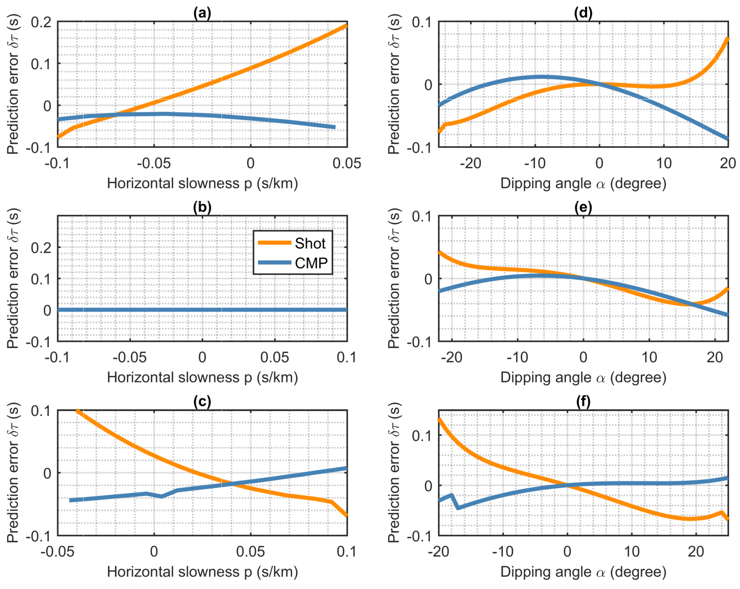
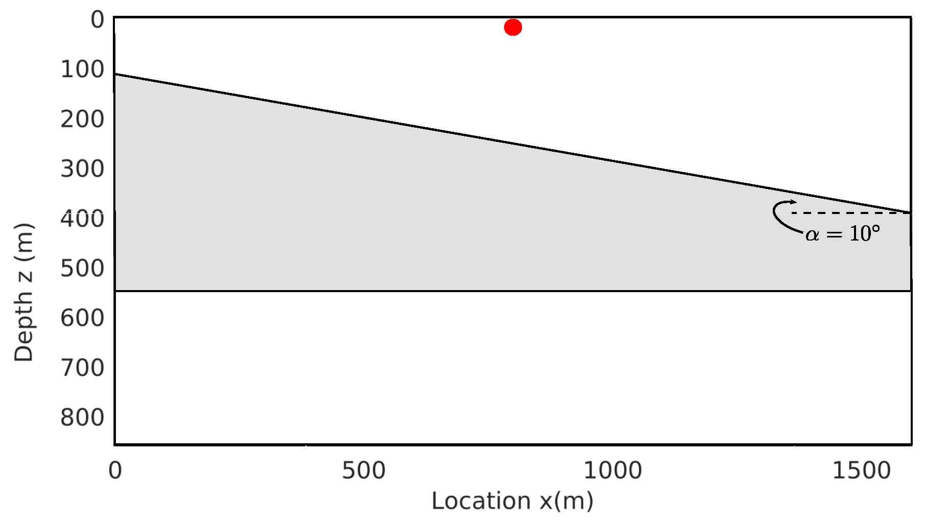
4. Numerical Analysis of the 1.5D Prediction Algorithm on the 2D Cases

Before implementing internal multiple prediction using the 1.5D algorithm with dipping strata, it is necessary to investigate the inclination dependency of the 1.5D algorithm and to discuss the performance differences using different input types. To do this, while ensuring the simplicity of calculation, we create a two-interface model, where the shallower reflector is slant with a dipping angle $\alpha$ (here, $\alpha >0$ if the depth of the interface increases from left to right and vice versa), while the deeper one is flat. In addition, we numerically simulate all ray-paths of primaries and the first-order internal multiples on a two-interface model, as shown in Figure 2 or Figure 3.

4.1. Error Analysis with the Shot Gathers

For a common shot gather, under a fixed source location and a fixed thickness of the top interface below the source point ($z_s=400$ m), the ray-paths of the three related events shown in Figure 2 are simulated with varying offsets x and dipping angles $\alpha$. In addition to the traveltimes of all ray-paths, the receiver-side horizontal slowness is also calculated for a certain offset x with a receiving angle ${\theta }_g$, i.e., $p_g=\frac{sin{\theta }_g}{c_0}$. Therefore, using Equation (4), the vertical traveltime (to distinguish with the one in the CMP gather, here, it is indicated as ${\tau }_s$) coherent to a fixed $p_g$ can be achieved as ${\tau }_s=t-p_{g}x$.

The vertical traveltimes of three events extracted from the common shot gathers in Figure 2 are plotted in Figure 4a. The top one represents the vertical traveltimes of the first primary reflections, which are indicated in green in Figure 2, with varying dipping angles and receiver-side horizontal slownesses $p_g$. The middle one delineates the vertical traveltimes of the second primary events, which are indicated in red in Figure 2. The bottom one represents the vertical traveltimes of internal multiples shown as the black event in Figure 2.

With the 1.5D prediction algorithm, the vertical traveltimes of the internal multiples are predicted by doubling the vertical traveltimes of the second primary events and then subtracting the vertical traveltimes of the first primaries, i.e., ${\tau }_{black}=2{\tau }_{red}-{\tau }_{green}$. Compared to the recorded internal multiples, the predicted errors with varying dipping angles $\alpha$ and horizontal slowness $p_g$ are plotted in Figure 4b. Figure 4b demonstrates that for a common shot gather internal multiple prediction on dipping strata using the 1.5D algorithm, the absolute values of prediction errors dramatically raised (up to 0.2 s) along the increasing dipping angles and horizontal slownesses.

4.2. Error Analysis with the CMP Gathers

To analyze the behaviors of the 1.5D prediction algorithm with the CMP gathers on dipping strata, we also simulate all ray-paths and compute the traveltimes of three reflection events in Figure 3 with varying offsets and dipping angles. With a fixed CMP location and a fixed thickness of the top interface below the CMP ($z_M=400$ m), the obtained traveltimes are sorted into the common average horizontal slowness $p_H$ manner, i.e., ${\tau }_M=t-p_{H}x$. Here, ${\tau }_M$ represents the relative vertical traveltimes related to the CMP location and the average horizontal slowness $p_H$.

Figure 5a shows the vertical traveltimes ${\tau }_M$ of primaries and internal multiples extracted from the CMP gathers, whose relationships are shown in Figure 3. The top one corresponds to the first primary indicated in green in Figure 3; the middle one represents the second primary indicated in red in Figure 3; and the bottom one delineates the vertical traveltimes of the first-order internal multiples with varying dipping angles $\alpha$ and average horizontal slownesses $p_H$, respectively. Based on Equation (3), the vertical traveltimes of internal multiples can be predicted by a lower–higher–lower combination over a fixed average horizontal slowness $p_H$. The prediction errors using the CMP gather along varying dipping angles and average horizontal slownesses are plotted in Figure 5b. As indicated in Figure 5b, except for the condition of around $\alpha =-{20}^{°}$ and $p_H=0.2$ s/km, the predicted errors remains in the range of $[-0.05,0.06]$, which are much smaller than the prediction errors of using the common shot gathers.

The comparisons of the predicted errors using the shot gathers and the CMP gathers, to be analyzed instinctively, are extracted at fixed dipping angles and at fixed horizontal slownesses, respectively. Figure 6a–c show the predicted errors of using the shot and the CMP gathers at the fixed dipping angle $\alpha =(-{25}^{°},0^{°},{25}^{°})$, separately, where the errors of the shot domain predictions are indicated in orange, and the errors of the CMP domain predictions are illustrated in dark blue.

In Figure 6a, with the fixed dipping angle $\alpha =-{25}^{°}$, the errors of the shot domain internal multiple predictions approximate linearly rise, while the predicted errors in the CMP domain remain in a relatively smaller range. Figure 6b shows the prediction errors in the shot and CMP domain with $\alpha =0^{°}$, i.e., a layered case. As indicated previously, under assumptions of layered media, the 1.5D prediction algorithm is able to predict accurate traveltimes of internal multiples on both the shot and the CMP gathers. In Figure 6c, the predicted errors are calculated with $\alpha ={25}^{°}$. Similar to Figure 6a, comparing with the prediction errors of using the shot gathers, implementing the 1.5D prediction algorithm in the CMP domain produces much more stable and independent results with varying horizontal slownesses, even under a large dipping angle condition.

The prediction errors of using the shot and CMP gathers at the fixed horizontal slowness $p=(-0.1,0.0,0.1)$ s/km are also extracted and plotted in Figure 6d–f, respectively. All predicted errors both in the shot and the CMP domain are zeros at dipping angle $\alpha =0^{°}$ in Figure 6d–f, which agrees with the fact in Equation (3). However, at the fixed horizontal slowness, the prediction errors of using the shot and the CMP gathers do not show the linear relationship with varying dipping angles, and limited advantages may be found in the CMP domain.

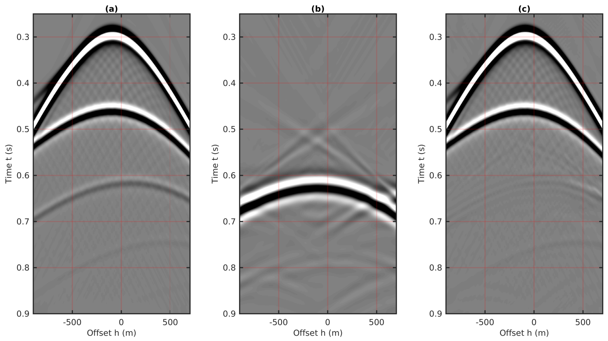
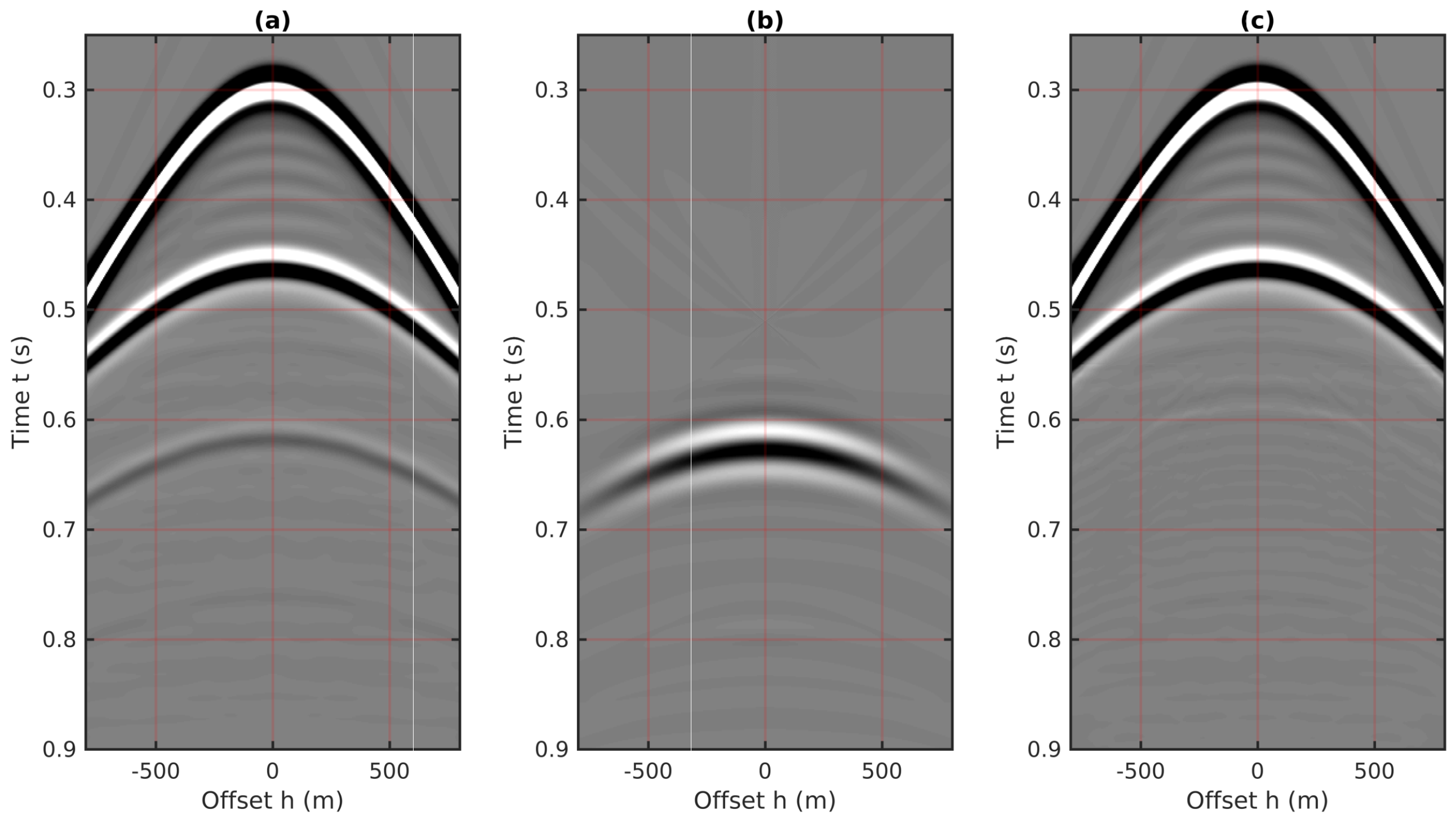
5. Numerical Examples

The inverse scattering series internal multiple prediction algorithm indicates that the prediction process is model independent, which means no prior model information is required during prediction. In other words, for acoustic cases, the complexity of the model does not affect the performance of the prediction algorithm; for elastic cases, a detailed discussion can be found in [27]. Therefore, in order to simplify the calculation and facilitate the analysis, we choose layered models with a tiltled reflector for numerical analysis and verification.

5.1. Two-Dimensional (2D) Prediction Using the 1.5D Algorithm

In this subsection, we numerically evaluate the performance of implementing the 1.5D prediction algorithm on the 2D cases. To do so, a three-layer model with one dipping reflector and one flat reflector is created and plotted in Figure 7. The velocities from top to bottom are (2200, 3500, 2200) m/s, and the dipping angle of the top interface is ${10}^{°}$. A total of 640 shot gathers are generated with source locations moving from left to right and occupying each receiver location. All sources and receivers with a fixed interval of 2.5 m are located at the top surface of the model. The internal multiples generated by three reflectors in Figure 7 are reconstructed using the 1.5D prediction algorithm with the shot gathers and the CMP gathers, respectively, for comparison.

We first perform the 2D internal multiple predictions using the 1.5D algorithm with the common shot gathers, where the source location is placed in the middle of the top surface of the model, which is shown as the red dot in Figure 7. The selected shot gather and the predicted internal multiple are plotted in Figure 8a,b, respectively. A non-stationary least-square subtraction is applied to remove the multiples from shot records, as shown in Figure 8c. We observe that the 2D internal multiples prediction using the 1.5D algorithm in the shot domain loses accuracy, especially at large offsets. For example, in Figure 8b, the predicted traveltime of the first-order internal multiple at the largest negative offset ($h=-800$ m) is less than 0.7 s, which is inconsistent with the 0.7 s in the original shot record shown in Figure 8a. At the largest positive offset ($h=800$ m), the traveltime of first-order internal multiple in the original shot gather is about 0.65 s; however, the predicted traveltime is at about 0.7 s. In Figure 8c, after the adaptive subtraction, the first-order internal multiples are removed at the near offset, but there are still residuals at the far offset. The numerical example in Figure 8 shows that the 2D internal multiples cannot be accurately predicted using the 1.5D algorithm in the shot domain due to the independence of horizontal slowness caused by the tilted reflector, which is consistent with our previous prediction error analysis.

Next, we implement the 2D internal multiple predictions using the 1.5D algorithm in the CMP domain. All 640 shot gathers are sorted into the CMP domain. The CMP gather with the midpoint located at the same location as the previous sot-domain experiment, i.e., the red dot in Figure 7, is extracted as an example and plotted in Figure 9a. Figure 9b shows the predicted results of the 2D internal multiples with the CMP gather using the 1.5D algorithm. In Figure 9b, the predicted traveltime of the first-order internal multiple is about 0.6 s at zero-offset and is around 0.69 s at the largest offsets ($h=\pm 800$ m), which are consistent with the original shot record. Figure 9c shows the primary events after the non-stationary least square subtraction.

Compared to the predictions using the shot gather, the 2D internal multiples generated by the tilted reflectors are well predicted using the 1.5D algorithm in the CMP domain at both near and far-offsets. The underlying reason is that due to the averaged horizontal slowness, the internal multiples in the CMP gathers exhibit better symmetry characteristics than in the shot gathers. Therefore, we may summarize that in the 2D cases of strata with nearly layered or small tilt angles, internal multiples can be efficiently reconstructed using the 1.5D prediction algorithm in the CMP domain with acceptable errors. Furthermore, the 2D internal multiples prediction using the 1.5D algorithm in the CMP domain is implemented on a trace-by-trace basis, which means that it can be easily performed using high-performance parallel computing. For reference, the runtime for implementing internal multiple predictions for a seismic trace with 901 time samples using Matlab is approximately 0.072 s on the i9 processor.

5.2. Two-Dimensional (2D) Prediction Using the 2D Algorithm

Our numerical analysis and implementation indicate that for internal multiple predictions with tilted strata, the CMP domain implementation of the 1.5D algorithm is relatively more tolerant than its shot–receiver domain implementation, benefiting from the averaged horizontal slowness. However, as indicated in the numerical analysis, the accuracy of the traveltime prediction for internal multiples using the 1.5D algorithm, even with the CMP gathers, is greatly reduced when the inclination of the reflector is very large. The 2D algorithm is suggested for a better 2D prediction of internal multiples caused by the large dip strata in the CMP gathers.

In this subsection, the use of Equation (9) with the CMP gathers in the coupled plane-wave domain for the full 2D internal multiples prediction is considered. The velocity model contains three layers and two reflectors, one flat interface and one dipping in 30 degrees, as shown in Figure 10. From the top to bottom, velocities are (2200 m/s, 2800 m/s, 4200 m/s). A total of 160 geophones with 2.5 m intervals are embedded 10 m below the surface, and shot records are generated with a 25 Hz Ricker wavelet for source locations moving from left to right and occupying each geophone location. A benchmark 2D synthetic reflection dataset is created using a fourth-order finite-difference forward modeling with acoustic constant density and four absorbing boundaries. The source–receiver–time volume of multishot records, after removing direct waves, is shown in Figure 11.

The multishot records are resorted in the CMP domain with the CMP-offset-time coordinate and illustrated in Figure 12. To observe the 2D character of the data in the CMP domain, we extract three CMP gathers from the resorted CMP volume, and they are plotted in Figure 13. As shown in Figure 13, two primaries and the first-order internal multiples are clearly visible in the three CMP gathers. Moreover, we also extract three shot gathers from the data volume in Figure 11, where the sources are in the same locations as the three CMPs shown in Figure 13. The three extracted shot gathers are plotted in Figure 14. Compared to the shot gathers in Figure 14, the reflection events in the CMP gathers with the large inclination strata show strong symmetry with respect to the offset, as shown in Figure 13. However, we will next show that this property of symmetry does not improve the accuracy of the traveltime predictions of internal multiples in the CMP domain using the 1.5D algorithm.

Before implementing the full 2D internal multiples predictions using the 2D algorithm, we first perform the predictions using the 1.5D algorithm with the three CMP gathers and the three extracted shot gathers, respectively. The final predictions for internal multiples in the CMP gathers and in the shot gathers are plotted in Figure 15 and Figure 16, respectively. Figure 15 and Figure 16 show that in the case of large dip strata, the 1.5D algorithm does not accurately predict the traveltimes of internal multiples neither in the CMP domain nor in the shot domain. Therefore, for the cases of large dip strata, the full 2D internal multiples prediction using the 2D algorithm is suggested.

Similar to the 2D plane-wave predictions in source–receiver coordinates, the coupled plane-wave transform is applied to the CMP data volume, which results in a 3D data volume with respect to the horizontal slownesses (i.e., $p_m$ and $p_h$, related to the CMP locations and half-offsets, respectively) and the vertical traveltime. Next, the transformed data volume is weighted by the factor $-\mathrm{i}2q_s$ to generate the final form of the input for the 2D prediction algorithm. Three common $p_m$ gathers extracted from this volume are plotted in Figure 17. Compared to the “butterfly” artifacts in the input related to source–receiver coordinates [26], the input of using the CMP gathers for internal multiples prediction has a similar aperture effects delineated as the cross-hyperbolic events in Figure 13, which can be eliminated by applying an attenuation taper on the limited aperture. Details of attenuating these butterfly effects caused by the finite aperture of the offset in the plane wave transformation can be found in [26].

The full 2D internal multiple predictions for all the 160 CMP gathers are implemented in the coupled plane-wave domain $\tau -p_m-p_h$ using Equation (9). The inverse coupled plane-wave transformation is applied to achieve the final predictions of internal multiples in the CMP-offset-time coordinates. The 2D predictions of internal multiples for the three CMP gathers shown in Figure 13 are extracted from the predicted volume and plotted in Figure 18. Comparing Figure 13 and Figure 18, we conclude that the multidimensional predictions can also be carried out in the CMP domain, which is able to capture the accurate arrival times of all possible internal multiples generated by large dip strata.

6. Conclusions

Internal multiples caused by the unknown generators can be predicted by the inverse scattering series internal multiple prediction algorithm in an automatic manner, which is usually performed on shot records with the source–receiver-related coordinates. For tilted strata, the algorithm requires multishot records occupying each receiver location, which greatly enhances the difficulty of input preparation and increases the computational cost. In this paper, we investigate the behavior of the 1.5D prediction algorithm in the cases of titled strata using the shot records and the CMP gathers, respectively. The numerical analysis of the prediction errors shows that the traveltimes of internal multiples generated by the titled reflector with small inclination can be predicted in the CMP domain using the 1.5D algorithm with acceptable errors compared to the predictions with the shot gathers. This is later verified by numerical examples of internal multiple predictions using the 1.5D algorithm with synthetic datasets. However, both numerical analysis and examples show that the 1.5D algorithm is not suitable for internal multiple predictions in the cases of large dip strata either with the shot records or in the CMP domain. To accommodate internal multiple predictions with the CMP gathers in complex environments, we also propose a modification of the multidimensional inverse scattering series internal multiple prediction algorithm that can be performed with the CMP gathers in the coupled plane-wave domain. The capacity of the modified multidimensional internal multiple prediction algorithm with the CMP gathers is validated by the benchmark synthetic example. We summarize that the implementation of internal multiple attenuation in the CMP domain may achieve better efficiency at approximate resolution, especially for cases with small inclination; however, its behavior in the elastic cases must be further investigated.

References

1. Alaei, N.; Roshandel Kahoo, A.; Kamkar Rouhani, A.; Soleimani, M. Seismic resolution enhancement using scale transform in the time-frequency domain. Geophysics 2018, 83, V305–V314. [Google Scholar] [CrossRef]
2. Alaei, N.; Soleimani Monfared, M.; Roshandel Kahoo, A.; Bohlen, T. Seismic imaging of complex velocity structures by 2D pseudo-viscoelastic time-domain full-waveform inversion. Appl. Sci. 2022, 12, 7741. [Google Scholar] [CrossRef]
3. Foster, D.J.; Mosher, C.C. Suppression of multiple reflections using the Radon transform. Geophysics 1992, 57, 386–395. [Google Scholar] [CrossRef]
4. VerWest, B. Suppressing Peg-leg Multiples with Parabolic Radon Demultiple. In Proceedings of the 64th EAGE Conference & Exhibition, Florence, Italy, 27–30 May 2002. [Google Scholar]
5. Trad, D. Interpolation and multiple attenuation with migration operators. Geophysics 2003, 68, 2043–2054. [Google Scholar] [CrossRef]
6. Hampson, D. Inverse velocity stacking for multiple elimination. In SEG Technical Program Expanded Abstracts 1986; Society of Exploration Geophysicists: Houston, TX, USA, 1986; pp. 422–424. [Google Scholar]
7. Lumley, D.E.; Nichols, D.; Rekdal, T. Amplitude-preserved multiple suppression. In Proceedings of the 1995 SEG Annual Meeting. Society of Exploration Geophysicists, Houston, TX, USA, 8–13 October 1995. [Google Scholar]
8. Yilmaz, Ö. Seismic Data Analysis; Society of Exploration Geophysicists Tulsa: Houston, TX, USA, 2001; Volume 1. [Google Scholar]
9. Zhang, N.; Wang, Y. An Inverse Data Space Method for Interbed Multiple Attenuation in the CMP Domain. In Proceedings of the 73rd EAGE Conference and Exhibition Incorporating SPE EUROPEC 2011, Vienna, Austria, 23–27 May 2011. [Google Scholar]
10. Berkhout, A. Seismic processing in the inverse data space. Geophysics 2006, 71, A29–A33. [Google Scholar] [CrossRef]
11. Staring, M.; Wapenaar, K. Three-dimensional Marchenko internal multiple attenuation on narrow azimuth streamer data of the Santos basin, Brazil. Geophys. Prospect. 2020, 68, 1864–1877. [Google Scholar] [CrossRef] [PubMed]
12. Zhang, L.; Slob, E. A field data example of Marchenko multiple elimination. Geophysics 2020, 85, S65–S70. [Google Scholar] [CrossRef] [Green Version]
13. Santos, R.S.; Revelo, D.E.; Pestana, R.C.; Koehne, V.; Barrera, D.F.; Souza, M.S.; Silva, A. An application of the Marchenko internal multiple elimination scheme formulated as a least-squares problem. Geophysics 2021, 86, WC105–WC116. [Google Scholar] [CrossRef]
14. Wapenaar, K.; Brackenhoff, J.; Dukalski, M.; Meles, G.; Reinicke, C.; Slob, E.; Staring, M.; Thorbecke, J.; van der Neut, J.; Zhang, L. Marchenko redatuming, imaging, and multiple elimination and their mutual relations. Geophysics 2021, 86, WC117–WC140. [Google Scholar] [CrossRef]
15. Thorbecke, J.; Zhang, L.; Wapenaar, K.; Slob, E. Implementation of the Marchenko multiple elimination algorithm. Geophysics 2021, 86, F9–F23. [Google Scholar] [CrossRef]
16. Dukalski, M.; de Vos, K. Overburden-borne internal demultiple formula. Geophysics 2022, 87, V227–V246. [Google Scholar] [CrossRef]
17. Ma, C.; Guo, M.; Liu, Z.; Sheng, J. Analysis and application of data-driven approaches for internal-multiple elimination. In SEG Technical Program Expanded Abstracts 2020; Society of Exploration Geophysicists: Houston, TX, USA, 2020; pp. 3124–3128. [Google Scholar]
18. Araújo, F.V.; Weglein, A.B.; Carvalho, P.M.; Stolt, R.H. Inverse scattering series for multiple attenuation: An example with surface and internal multiples. In Proceedings of the 64th Annual International Meeting SEG Expanded Abstracts, Los Angeles, CA, USA, 23–27 October 1994. [Google Scholar]
19. Weglein, A.B.; Gasparotto, F.A.; Carvalho, P.M.; Stolt, R.H. An inverse-scattering series method for attenuating multiples in seismic reflection data. Geophysics 1997, 62, 1975–1989. [Google Scholar] [CrossRef]
20. Luo, Y.; Kelamis, P.G.; Fu, Q.; Huo, S.; Sindi, G.; Hsu, S.Y.; Weglein, A.B. Elimination of land internal multiples based on the inverse scattering series. Lead. Edge 2011, 30, 884–889. [Google Scholar] [CrossRef]
21. Herrera, W.; Weglein, A.B. Eliminating first-order internal multiples with downward reflection at the shallowest interface: Theory and initial examples. In SEG Technical Program Expanded Abstracts 2013; Society of Exploration Geophysicists: Houston, TX, USA, 2013; pp. 4131–4135. [Google Scholar]
22. Zou, Y.; Weglein, A.B. A new method to eliminate first order internal multiples for a normal incidence plane wave on a 1D earth. In Proceedings of the 2013 SEG Annual Meeting, Houston, TX, USA, 22–27 September 2013. [Google Scholar]
23. Ramirez, A.; Weglein, A. Progressing the analysis of the phase and amplitude prediction properties of the inverse scattering internal multiple attenuation algorithm. J. Seism. Explor. 2005, 13, 283–301. [Google Scholar]
24. Yang, J.; Weglein, A.B. Accommodating the source wavelet and radiation pattern in the internal multiple attenuation algorithm: Theory and initial example that demonstrates impact. In SEG Technical Program Expanded Abstracts 2015; Society of Exploration Geophysicists: Houston, TX, USA, 2015; pp. 4396–4401. [Google Scholar]
25. Innanen, K.A. Time-and offset-domain internal multiple prediction with nonstationary parameters. Geophysics 2017, 82, V105–V116. [Google Scholar] [CrossRef] [Green Version]
26. Sun, J.; Innanen, K.A. Multidimensional inverse-scattering series internal multiple prediction in the coupled plane-wave domain. Geophysics 2018, 83, V73–V82. [Google Scholar] [CrossRef]
27. Sun, J.; Innanen, K.A. A plane-wave formulation and numerical analysis of elastic multicomponent inverse scattering series internal multiple prediction. Geophysics 2019, 84, V255–V269. [Google Scholar] [CrossRef]
28. Sun, J. Computational and Practical Developments in Single-and Multi-Component Inverse Scattering Series Internal Multiple Prediction. Ph.D. Thesis, University of Calgary, Calgary, AB, Canada, 2018. [Google Scholar]
29. Coates, R.; Weglein, A. Internal multiple attenuation using inverse scattering: Results from prestack 1 & 2D acoustic and elastic synthetics. In SEG Technical Program Expanded Abstracts 1996; Society of Exploration Geophysicists: Houston, TX, USA, 1996. [Google Scholar]
30. Ocola, L.C. A nonlinear least-squares method for seismic refraction mapping-Part II: Model studies and performance of Reframap method. Geophysics 1972, 37, 273–287. [Google Scholar] [CrossRef]
31. Diebold, J.B.; Stoffa, P.L. The traveltime equation, tau-p mapping, and inversion of common midpoint data. Geophysics 1981, 46, 238–254. [Google Scholar] [CrossRef]
Figure 1. Ray-path schematic of primaries (dashed line) and internal multiple (solid line) with corresponding source and receiver locations. See also [29].
Remotesensing 15 03002 g001
Figure 2. Combinations of events in a common shot gather for internal multiple prediction using the 1.5D algorithm. Both primaries and internal multiples shared the same horizontal slowness corresponding to the receiver side, i.e., p g .
Remotesensing 15 03002 g002
Figure 3. Combinations of events in a CMP gather for internal multiple prediction using the 1.5D algorithm. All events in the combination share the same average horizontal slowness, i.e., p H = p g + p s 2 = p g 1 + p s 1 2 = p g 2 + p s 2 2 .
Remotesensing 15 03002 g003
Figure 4. Error analysis of implementing the 1.5D algorithm on the 2D cases with the common shot gathers. (a) Vertical traveltimes of three events, shown in Figure 2, extracted from a common shot gather with varying dipping angles α and horizontal slownesses p g , i.e., the top one represents the vertical traveltimes of the 1st primary reflection, indicated in green in Figure 2; the middle one shows the vertical traveltimes of the 2nd primary event, indicated in red in Figure 2; the bottom one delineates the vertical traveltimes of the internal multiples shown in Figure 2. (b) Prediction errors with shot gathers using the 1.5D prediction algorithm.
Remotesensing 15 03002 g004
Figure 5. Error analysis of implementing the 1.5D algorithm on 2D cases with the CMP gathers. (a) Vertical traveltimes of three events, shown in Figure 3, extracted from the CMP gather with varying dipping angles α and average horizontal slownesses p H , i.e., the top one represents the vertical traveltimes of the 1st primary reflection, which are indicated in green in Figure 3; the middle one shows the vertical traveltimes of the 2nd primary event, which are indicated in red in Figure 3; the bottom one delineates the vertical traveltimes of the internal multiple shown in Figure 3. (b) Prediction errors with the CMP gathers using the 1.5D prediction algorithm.
Remotesensing 15 03002 g005
Figure 6. Comparisons of the predicted errors using the shot and the CMP gathers at the fixed dipping angle α = ( 25 ° , 0 ° , 25 ° ) and at the fixed horizontal slowness p = ( 0.1 , 0.0 , 0.1 ) s/km, respectively. The prediction errors of using shot gathers are indicated in orange, and those of using the CMP gathers are illustrated in dark blue. (a) Comparisons of prediction errors at α = 25 ° with varying p. (b) Comparisons of prediction errors at α = 0 ° with varying p. (c) Comparisons of prediction errors at α = 25 ° with varying p. (d) Prediction errors at p = 0.1 s/km with varying α . (e) Prediction errors at p = 0.0 s/km with varying α . (f) Prediction errors at p = 0.1 s/km with varying α . Note, for the shot gathers, p represents p g ; for the CMP gathers, p represents p H .
Remotesensing 15 03002 g006
Figure 7. A two-interface model with one dipping reflectors and one flat reflector. The dipping angle of the top interface is 10 ° . Here, the red dot indicates the source location for the common shot gather, and it represents the CMP location for the CMP gather.
Remotesensing 15 03002 g007
Figure 8. The 2D internal multiple prediction with the common shot gather using the 1.5D algorithm. (a) The shot gather created using the velocity model shown in Figure 7 with the source location indicated as the red dot. (b) The internal multiple prediction using Equation (3). (c) The shot gather after the least-square matching subtraction, i.e., c = a-factor*b.
Remotesensing 15 03002 g008
Figure 9. The 2D internal multiple prediction using the CMP gather using the 1.5D algorithm. (a) The CMP gather created using the velocity model shown in Figure 7 with the CMP location indicated as the red dot. (b) The internal multiple prediction using Equation (3). (c) The CMP gather after the least-square matching subtraction, i.e., c = a-factor*b.
Remotesensing 15 03002 g009
Figure 10. The geological model with two interfaces, including one flat reflector and one dipping reflector. The dipping angle of the second interface is 30 ° . From the top to bottom, velocities are (2200 m/s, 2800 m/s, 4200 m/s). Locations of sources and receivers are delineated as stars and triangles, respectively.
Remotesensing 15 03002 g010
Figure 11. Multishot records sorted in the source–receiver–time coordinate with the velocity model shown in Figure 10.
Remotesensing 15 03002 g011
Figure 12. Multishot records sorted in the CMP-offset-time coordinate.
Remotesensing 15 03002 g012
Figure 13. Three CMP gathers extracted from the CMP data volume shown in Figure 12. (a) The 40th CMP gather, (b) the 80th CMP gather, (c) the 120th CMP gather.
Remotesensing 15 03002 g013
Figure 14. Three common shot gathers extracted from the data volume in Figure 12, where the sources are in the same locations as the CMPs in Figure 13. (a) The 40th shot gather, (b) the 80th shot gather, (c) the 120th shot gather.
Remotesensing 15 03002 g014
Figure 15. Internal multiple predictions using the 1.5D algorithm with the three CMP gathers shown in Figure 13. (a) The 40th CMP gather, (b) the 80th CMP gather, (c) the 120th CMP gather.
Remotesensing 15 03002 g015
Figure 16. Internal multiple predictions using the 1.5D algorithm with the three shot gathers shown in Figure 13. (a) The 40th shot gather, (b) the 80th shot gather, (c) the 120th shot gather.
Remotesensing 15 03002 g016
Figure 17. Three common p m gathers extracted from the τ p m p h transformed CMP volume. (a) p m = 0.2 s/km. (b) p m = 0 s/km. (c) p m = 0.2 s/km.
Remotesensing 15 03002 g017
Figure 18. The 2D internal multiples predictions using the 2D algorithm for the three CMP gathers shown in Figure 13. (a) The 40th CMP gather, (b) the 80th CMP gather, (c) the 120th CMP gather.
Remotesensing 15 03002 g018
Disclaimer/Publisher’s Note: The statements, opinions and data contained in all publications are solely those of the individual author(s) and contributor(s) and not of MDPI and/or the editor(s). MDPI and/or the editor(s) disclaim responsibility for any injury to people or property resulting from any ideas, methods, instructions or products referred to in the content.