1. Introduction
Oil spill accidents frequently occur when offshore oil is being exploited and transported overseas. The oil spill risk is quickly rising as the need for crude oil increases. After an oil spill accident happens, spilled oil will usually rise to the sea surface and generate an oil slick due to it having a lower density than water. An oil slick usually causes long-term hazardous effects on the sea environment [
1,
2,
3], including disrupting the marine ecosystem and causing the deaths of many marine organisms.
In order to effectively reduce the effects of spilled oil on the marine environment, efficient oil spill response methods and techniques have to be developed. The methods for removing spilled oil from marine environments include mechanical recovery [
4], dispersant dissolving and in situ burning (ISB) [
5,
6]. The oil slick volume is very important information that usually determines the choice of the oil spill response option, the calculation of oil spill disposal efficiency, and even the amounts of fines issued to the responsible party. In order to obtain the volume information, both the oil spill thickness and area have to be accurately measured. Many methods have been proposed for measuring the thickness within different ranges based on different techniques [
7]. Basically, the techniques can be divided into two types: remote sensing methods and contact-based methods.
Remote Sensing Methods
There are several remote sensing techniques that can be used for estimating the thickness of an oil slick, including visual observation [
8,
9,
10], hyperspectral imaging [
11,
12,
13,
14], and laser ultrasound [
15,
16,
17].
Visual observation is one of the simplest methods used to detect oil spills. In this technique, an experienced expert estimates the thickness based on color observations by from airborne platforms [
9]. It can only be implemented to estimate the thin sheen thickness (<100 μm) [
8]. The accuracy can be severely influenced by light reflections, sea conditions, atmospheric and viewing conditions, etc. [
10].
Hyperspectral imaging is also widely applied for detecting oil spills [
11,
12,
13,
14]. This technique involves estimating oil slick thickness based on the relationship between the oil spill hyperspectral reflectance and thickness. However, the accuracy can be heavily impacted by sea states and weather conditions. In addition, this technique cannot be applied to measure thick oil slick thickness.
Laser ultrasound is another technique that can be deployed to remotely measure oil slick thickness by multiplying the ultrasonic traveling time within the oil slick by assessing the speed of sound. A laser ultrasonic remote sensor was developed by Brown et al. [
15,
16,
17] to measure oil slick thickness using an airplane as the platform, and many tests were conducted to validate this technique. However, the sensing system was so expensive and complex that it was not widely deployed in the field. In addition, like other remote sensing methods, the accuracy was also dependent on atmospheric conditions, such as clouds and oil weathering.
Recently, some other new techniques such as thermal remote sensing [
18], radar backscatter [
19], and water Raman suppression [
20] were also proposed. In technical terms, there is still a great challenge in applying remote sensing methods for measuring thick oil slick thickness.
Contact-Based Methods
Besides remote sensing techniques, many scholars have investigated several contact-based methods for measuring oil thickness. Massaro et al. [
21] developed an optical-based sensor to detect oil and estimate the oil thickness according to the relationship between the intensity of reflected light and the thickness. The dependence of the sensitivity of the sensor on the optical properties of oils was examined. An electric conductivity sensor with a metallic array, developed by Denkilkian et al. [
22], was investigated to determine its ability to measure the oil thickness based on the lower electric conductivity of oil in comparison to seawater. However, the sensor had a very low resolution, and it could not be used for oil fouling in dynamic environments. Saleh et al. [
23] developed a capacitive-based sensor and conducted experiments at the Ohmsett with sea waves. The experimental results showed that the sensor could be deployed for in situ measurement of thick oil slick thickness, although the measurement accuracy was relatively low. Technically, contact-based sensors also face significant challenges in accurately measuring oil slick thickness in the oil spill field. Recently, Du et al. [
24] proposed the utilization of a remotely operated vehicle (ROV) as a platform for measuring thick oil slick thickness with ultrasound. The measurement accuracy of this method was fully verified in laboratory measurements.
Accurately measuring the area of an oil spill has great significance for rapid responses to oil spill accidents. Many scholars are committed to proposing fast and effective algorithms for detecting oil spill areas. Tejaswini et al. [
25] proposed an edge detection algorithm to detect the area of an oil spill in a synthetic aperture radar (SAR) image and achieved excellent detection results. Cantorna et al. [
26] applied clustering, logistic regression and convolutional neural network (CNN) algorithms for detecting oil leakage by processing satellite images. They found that the logistic regression and clustering algorithms could be used for oil leakage segmentation, and that the CNN achieved the best results in low computing times. With the rapid advancement of deep learning technology, some scholars in related fields have used this technology to process SAR images in order to measure oil spill area. Zhang et al. [
27] used an R-CNN network to extract SAR image features and identify oil spill areas. Liu et al. [
28] proposed a black spot detection method to identify oil spill areas with high accuracy based on a superpixel depth map convolution network method.
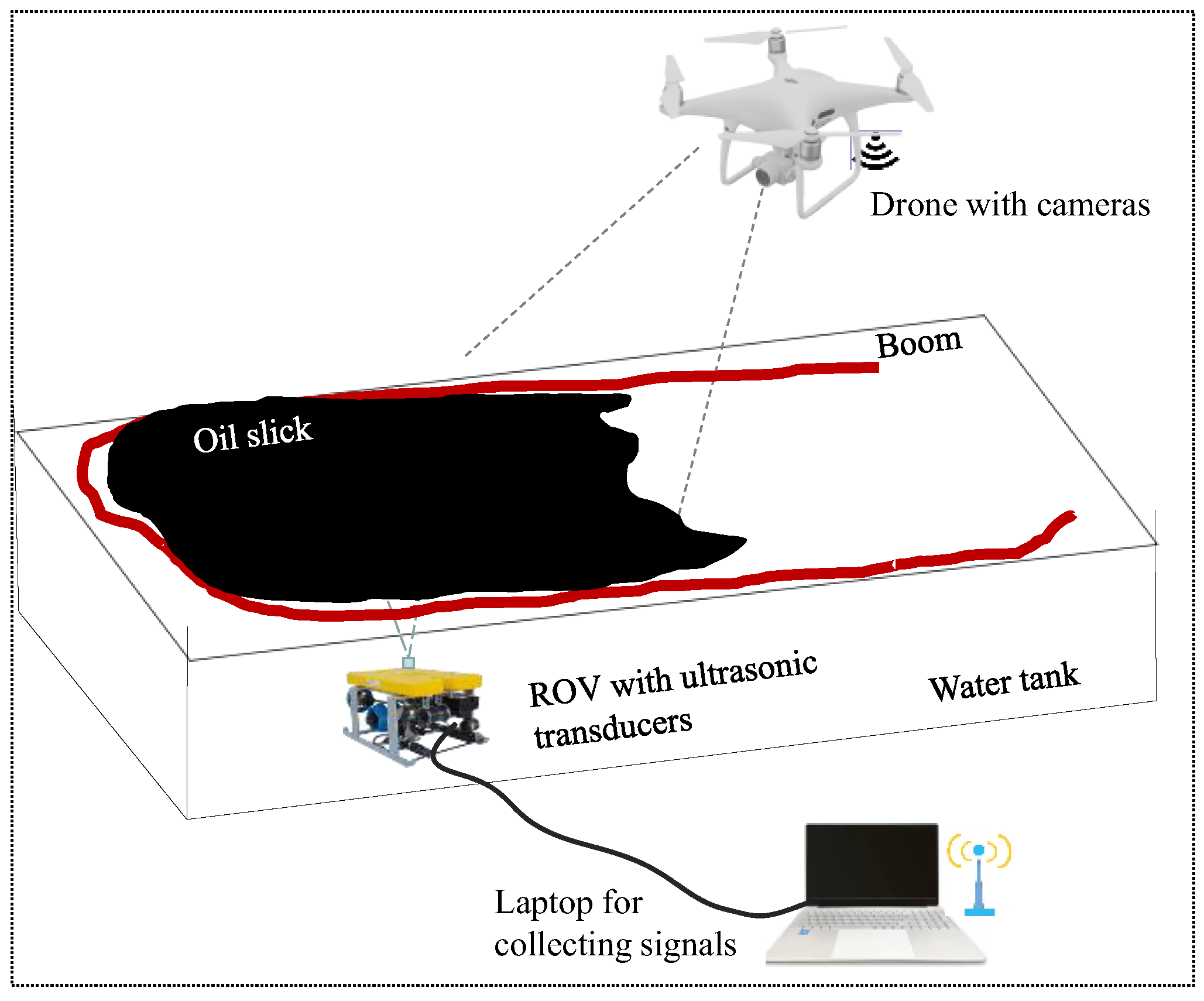
In this article, a method is proposed to measure oil slick volume by combining the measurements of the thickness and area of an oil slick with ultrasound and image processing. These aspects are assessed using an ROV and an airborne drone as platforms, respectively. An ROV carrying two ultrasonic immersion transducers was used to assess oil slick thickness by multiplying the ultrasonic time of flight (TOF) within the oil slick by the speed of sound. A six-rotor drone was used to capture optical images of the oil slick. The area of the oil slick was assessed by performing a series of image processing steps on optical images of the oil slick. Multiple measurements were conducted to verify the proposed method.
2. Methodology
To overcome the difficulty of current methods [
11,
12,
13,
14,
15,
16,
17,
18,
19,
20] in measuring the thickness of thick oil slicks and effectively solve the problem of accurately estimating the volume of oil slick prior to making the oil response strategies, a novel method of measuring the volume of oil slick is proposed in this article. This technique works by simultaneously measuring the thickness and area using ultrasonic inspection and image processing methods, with an underwater ROV and an airborne drone as platforms, respectively. An ROV carrying an ultrasonic inspection system with two transducers was controlled through a cable. We induced the ROV to freely move underneath an oil slick in order to continuously measure the thickness of the oil slick at multiple positions. An airborne drone with optical cameras was remotely controlled to continuously record videos of the oil slick, and an optical image processing algorithm was developed to measure the area of the oil slick. The capturing, saving and processing of ultrasonic and optical data were synchronized on the same laptop.
Technically, the experimental procedures included the following 5 steps.
- (1)
Crude oil with a density of 0.89 g/L, purchased from a local oil well (Liaoyang, Liaoning Province, China), was added into the water tank to generate a thick oil slick.
- (2)
A water pump was placed at the bottom of the tank and used to generate the driving force in order to continuously vary the area of the oil slick.
- (3)
An ROV carrying two ultrasonic transducers was deployed in the tank to freely move underneath an oil slick to capture ultrasonic reflections from the oil slick, while a drone with optical cameras was flown above the water tank to statically capture images of oil slicks.
- (4)
The ultrasonic and optical data were synchronously sent back and saved on a laptop. The thickness and area of the oil slick were simultaneously calculated by processing data using ultrasonic signal processing and image processing algorithms, respectively.
- (5)
The volume of the oil slick was easily measured by multiplying the thickness by the area of the oil slick.
- A.
Oil Slick Thickness Measurement
The thick oil slick thickness was measured by collecting ultrasonic reflections from interfaces between oil, water and oil due to acoustic impedance differences among the three fluids. The acoustic impedance,
Z, is defined by Equation (1)
where
ρ and
V are the density and the speed of sound of the fluid, respectively. The strengths of ultrasonic reflection from interfaces are highly dependent on the difference in acoustic impedance between the two fluids.
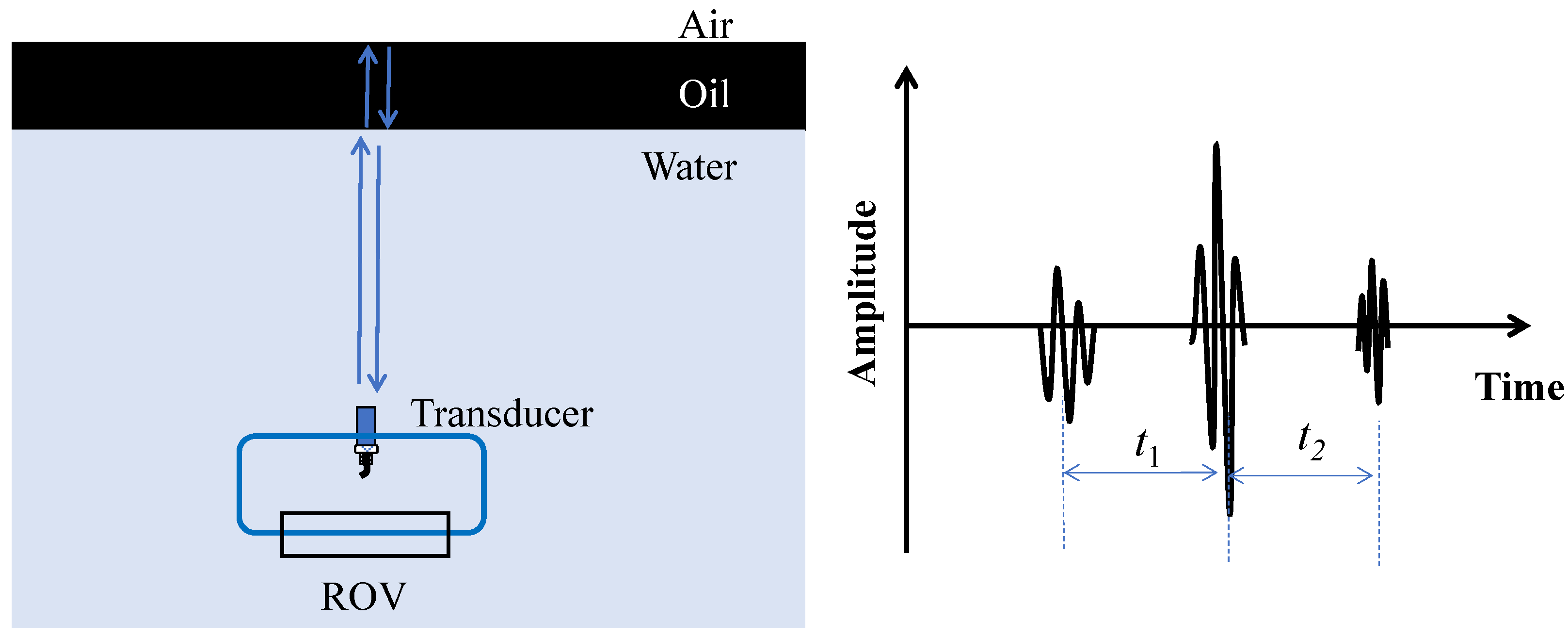
Figure 1 shows the schematic of receiving ultrasonic reflections underneath an oil slick using an ultrasonic transducer installed on a free-moving ROV platform. The ultrasonic transducer emits ultrasonic pulses and receives reflections from the oil slick. The ROV can be remotely controlled to measure oil slick thicknesses at any specific location. The right image shows a collected ultrasonic signal, in which the first, middle and last signals correspond to reflections from the bottom and top of an oil slick and the reverberation, respectively. It can be observed that the amplitude of the reflection from the top of oil slick (air–oil interface) is much higher than the amplitude of reflection from the bottom of oil slick (oil–water interface) [
24], which is attributed to the larger acoustic impedance difference existing between oil and air than the acoustic impedance difference between oil and water.
To measure the oil slick thickness, the ultrasonic traveling time within an oil slick has to be determined by calculating the time difference
t1 between reflections from the top and bottom of an oil slick. Technically, the time of flight (TOF)
t1 is equal to
t2 at the static condition. However, because of the surface vibration, the movement of the platform, and the ultrasonic attenuation, the reverberation is sometimes deeply decayed and undetectable. Therefore, the TOF
t1 is usually used to calculate oil slick thickness with Equation (2),
where
h represents the thickness of an oil slick, and
V is the speed of sound in oil.
- B.
Oil Slick Area Measurement
A six-rotor drone carrying a vertical down optical camera was used to capture images of the oil slick boomed within a water tank. The drone hovered above the water tank to record videos during experiments. The area of oil slick was changed by the driving force generated by a water pump that was placed at the bottom of the tank to pump water up to the surface in order to make the surface water flow. When the pump was turned off, the oil slick freely expanded the whole boomed area.
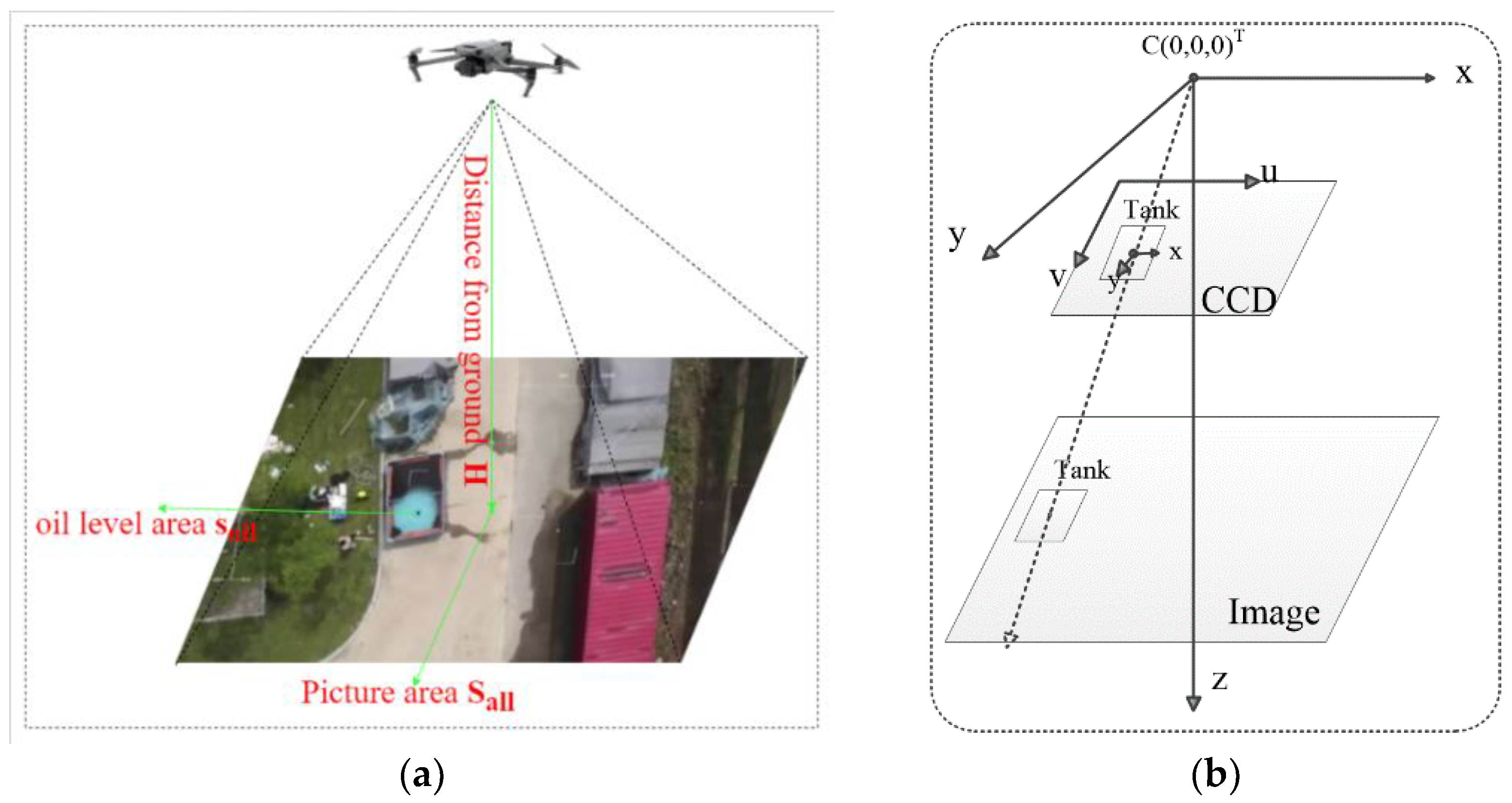
Figure 2 shows the schematic of capturing videos of oil slick with a drone.
Figure 2a describes the real drone acquisition scenario. In order to facilitate understanding our algorithm process, a coordinate map was drawn on
Figure 2b. A spatial coordinate axis was established with the drone as the origin
C(0,0,0)
T. The
x,
y, and
z axes represent the length, width, and height directions of the drone’s shooting range, respectively. A charge-coupled device (CCD) image sensor was used to project the actual landscape. The CCD size of the optical camera was 1/2.8 inch and the focal length f = 4.4 mm. The image resolution was 1920 × 1080 pixels, and the flight altitude
H of the drone was 18.2 m. The actual shooting area
of the camera was calculated to be around 319.3 m
2 according to the similar triangle theorem. The image data were wirelessly transmitted to the laptop and we performed specific image processing procedures to calculate the oil slick area. Since the oil slick area was continuously changing in an irregular shape when the pump was periodically turned on/off, and the lightness of oil slick edges in optical images was usually much stronger in comparison to other locations, it was very challenging to directly extract the oil slick area from optical images with the existing image processing algorithms. Therefore, a new image processing method was proposed to calculate the area of oil slick.
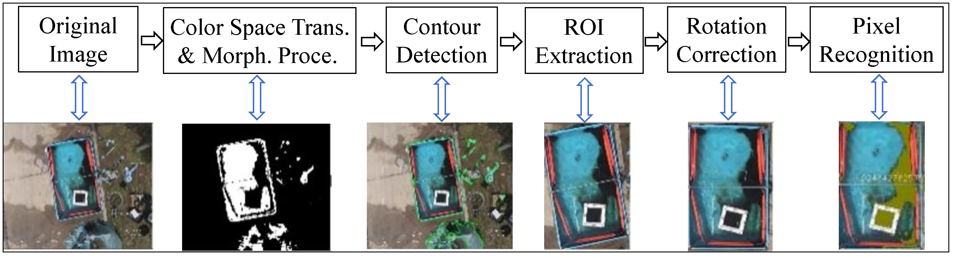
Figure 3 shows the procedures of measuring the oil slick area with the proposed image processing method. By analyzing images, the water tank and the surrounding environment were considered as the foreground and background, respectively. The color space transformation and morphological processing were performed on the entire image to separate the water tank from the environment. The color space transmission converted the RGB (red, green and blue) space into the HSV space to obtain binarized images. The morphological processing conducted the first dilation and then erosion on binarized images to fill small holes in objects, connect adjacent objects, smooth boundaries without changing the area and suppress noise details for the convenience of contour detection.
We obtained the binarized images for use in contour detection with the background being mostly masked out. The principle of contour detection is to track the target boundary and find all points to form the boundaries that can be used to accurately select the area of the water tank. The continuous and closed contour lines in the binary image were the search targets. The rectangle contour with the largest area among all the obtained contours was selected as the final water tank contour line for extraction.
The ROI extraction on the image was followed the contour detection process. The spatial relationship between the context and the object of interest could be accurately captured by the ROI extraction. Since the oil slick area was very small and was continuously changing in the pattern of an irregular shape, directly defining the oil spill area as ROI was a significant challenge. Therefore, the rectangular water tank was chosen as the ROI based on its regular rectangular shape, which can be well detected from the entire image. In addition, since the oil slick was fully contained in the water tank, and as there were no debris interferences in the water tank, the oil spill area was able to be easily separated after obtaining the outlines of the water tank. Then, a rotation correction algorithm was implemented to crop the image of the water tank based on the image edge. Affine changes were induced to deflect the image to render the cropped image in the horizontal position. It has been experimentally verified that the cropped image does not affect the resolution of the water tank in the original image.
Since the oil slick area and the image background area occupy different grayscale ranges, the threshold segmentation algorithm based on region pixels is used to separate the oil slick area from the normal water area by analyzing the grayscale difference between the extracted target and the background. The threshold is set to divide the pixel levels into several categories. Equation (3) is used to separate pixels of the clean water area from the oil slick area.
where
,
, and
indicate the thresholds of the image pixel RGB, respectively. The pixel is regarded as the oil when the R, G and B are all numerically smaller than
,
, and
. The number of oil slick pixels is counted and marked as
. Then, the oil spill area
can be calculated by Equation (4),
where
= 1920 × 1080 denotes the number of pixels in the whole image, and
= 319.3 m
2 denotes the actual imaging area captured by a drone.
3. Data Acquisition
The experiments were conducted in the laboratory to verify the proposed method.
Figure 4 shows the experimental schematic of measuring the thickness and the area of an oil slick using ultrasonic and image processing methods, respectively. The oil slick was boomed in the water tank. A small ROV carrying two ultrasonic immersion transducers was controlled to freely float underneath the oil slick at a constant depth. Ultrasonic signals reflected from the bottom and top of the oil slick were captured and saved on the laptop through cables. A drone with an optical camera was flown vertically above the water tank to capture videos during experiments. The optical data were wirelessly transferred to the laptop.
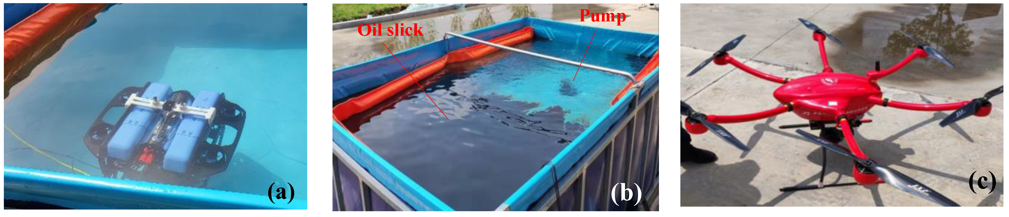
Figure 5a shows a small ROV (
BlueRobotics) with the maximum diving depth of 100 m and eight motors floating in the water tank with aconstant diving depth of ~30 cm before adding oil. Ultrasonic reflections from the oil slick were received by two ultrasonic immersion transducers purchased from
Olympus with 5 MHz central frequency. The transducers were installed on the ROV and connected with two channels of the 8-channel Micropulser (PeakNDT, British). The pulse–echo configuration was used, in which each transducer behaved as both the source and receiving transducers.
Figure 5b shows the water tank used in the laboratory experiment. The dimensions of this tank were 3 m (length) × 2 m (width) × 1 m (height). The tank was filled with fresh water up to the height of about 0.9 m. Crude oil with a density around 0.89 g/mL was used in the experiment. Initially, 10 L crude oil was added in the boomed area of about 180 cm × 280 cm in the water tank to generate an oil slick with a thickness of ~2.0 mm. Then, 5 more liters of oil was poured into the tank to increase the thickness of the oil slick. A water pump that was placed at the bottom of the water tank was used to vertically pump water up to drive the surface water flow, which resulted in the oil slick shrinking, as shown in
Figure 5b. When the pump was powered-off, the contracted oil slick slowly expanded to restore the whole boomed area. The area of the oil slick was changed by periodically switching the pump.
Figure 5c shows a six-rotor drone developed by the Institute of Automation of Shenyang for use in measurements. The six-rotor drone was remotely controlled to hover above the water tank at a height of ~18 m to capture videos of oil slicks using a visible light downward camera with a 1080 resolution and 30 times optical zoom capability. The field of the view angle was around 63.7 degrees, and the image resolution was 1920 × 1080.
Table 1 lists the major parameters of the ROV and the drone.
Ultrasonic data acquisition program was developed to collect ultrasonic signals. The ROV with two transducers freely drifted underneath the oil slick at a fixed depth to continuously collect ultrasonic data. The pulse width was set to 100 ns. The sampling rate was set 100 MH and the pulse repetition frequency was set 100 Hz. Electronic noises were reduced by averaging every 16 collections to make an ultrasonic signal. The sampling resolution was chosen to be 0.5 s/data. The number of collected data points was about 1200. The pump was periodically powered on/off every 50 s.
4. Data Analysis
Figure 6a shows the image of the collected 1200 ultrasonic signals received with one transducer. The color denotes the amplitudes of ultrasonic signals. The
x axis denotes the 600 s sampling time used during the experiment, while the
y axis denotes the travel time of ultrasound within water and the oil slick.
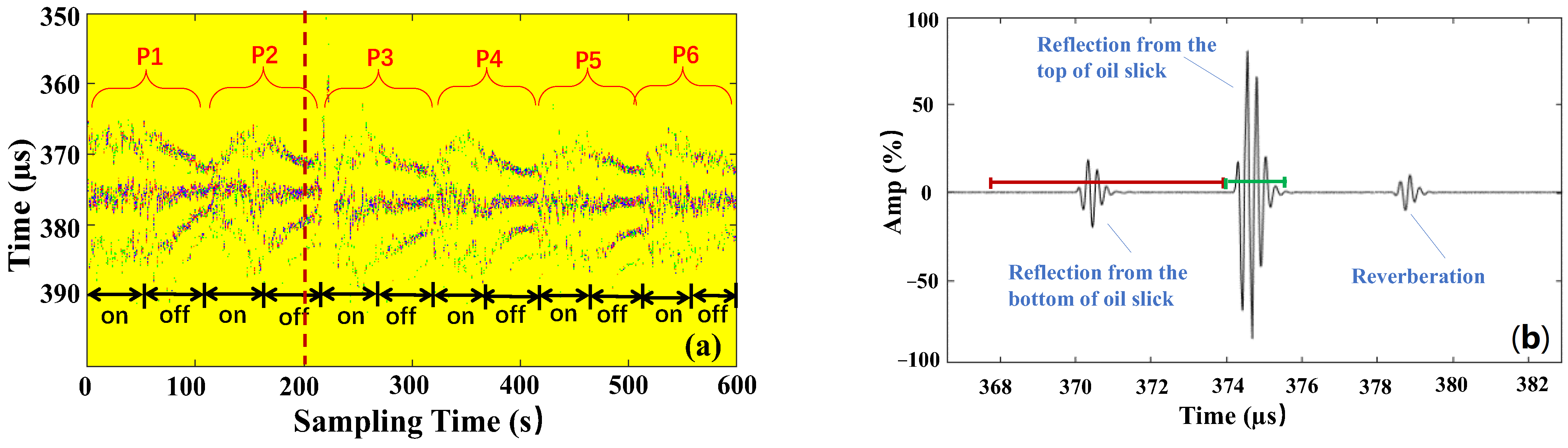
Figure 6b shows a representative ultrasonic signal corresponding to around ~200 s when the pump was turned off. This is marked with a dashed red line and can be seen in
Figure 6a. The reflections from the oil slick and the reverberation can be easily distinguished. It can be found that the reflection from the top of the oil slick was much stronger than the reflection from the bottom of the oil slick due to the larger acoustic impedance difference between air and oil in comparison to the acoustic impedance between water and oil. The pump was periodically powered on/off roughly every 50 s for six periods, marked as P1~P6. It can be seen that the time differences between two reflections were periodically decreasing and increasing with respect to the turning on/off of the pump in each period, respectively.
The collected ultrasonic signals were processed to obtain the TOF from within the oil slick. The cross-correlation method was implemented to assess the TOF by conducting the cross-correlation of the top and bottom reflections. As stated in Reference [
24], the largest difficult facing this method was the need to effectively and accurately separate these two reflections from each other. The difficulty rose as the thickness decreased. When the thickness of an oil slick was approaching the measurable thickness ~0.5 mm of a 5.0 MHz transducer, the reflections had the potential to fully or partially overlap so that they were barely separated. In this article, because the thickness of the oil slick was much higher than that of the measurable thickness, the two reflections could easily be distinguished from each other. Due to the higher reflection from the top of an oil slick, the reference point was chosen by picking the peak using a wide time gate with a threshold of around ~5%. When the peak was over the threshold, two gates were triggered to extract two reflections from the oil slick, respectively, as shown in
Figure 6b. The details regarding the gate setting are discussed in Reference [
24]. The green gate began around ~1.25 wavelengths prior to the reference point. To fully cover the top reflection, the length of the green gate was set at 4 wavelengths at least. For the red gate used to extract the bottom reflection, the end of the red gate was chosen as the start of the green gate. The length of the red gate was set widely to cover a wide thickness range. If the peak was lower than the threshold, this signal was not applicable.
The signals within two gates were firstly extended in the same time window. Then, the cross-correlation was operated to determine the TOF.
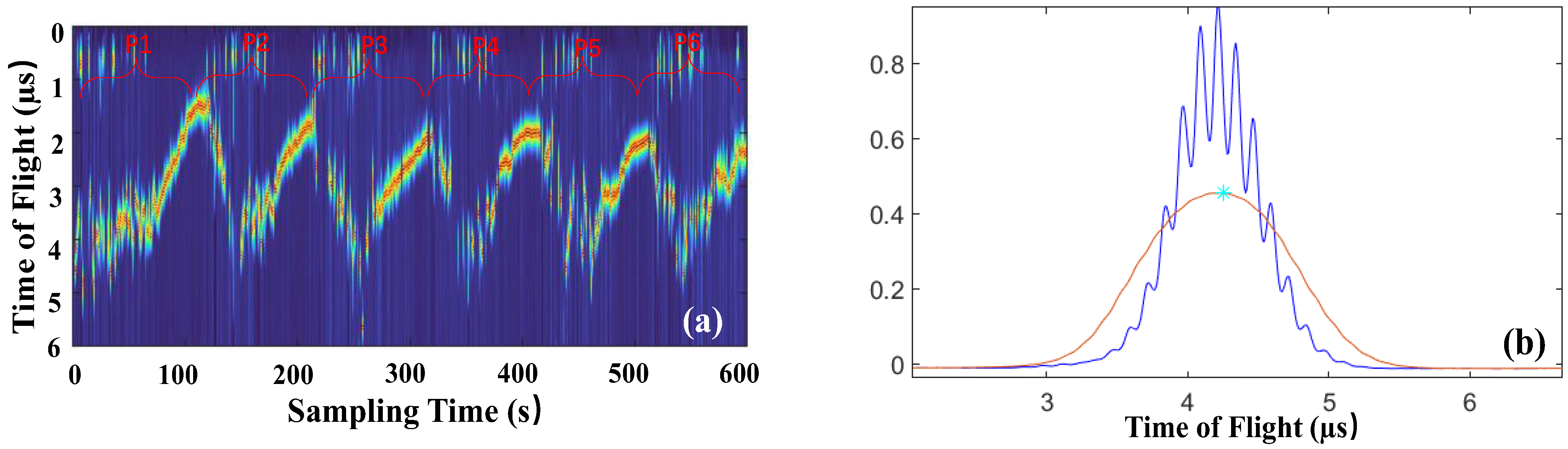
Figure 7a shows the normalized cross-correlation image. The
x axis indicates the sampling time, as shown
Figure 6a, while the
y axis represents the time of flight. The TOF periodically changed as the pump was periodically switched on/off. When the pump was turned on, the TOF dynamically shifted due to the surface water flow. When the pump was powered off, the TOF decreased almost linearly. In addition, the slope of the varying TOF was nearly identical in each period, a value that may be used to study the expansion rate of an oil slick.
Figure 7b shows a normalized cross-correlation of two extractions and a fit curve at ~150 s. The TOF of
t1 = 4.25 µs was determined by assessing the peak of the fit curve. The thickness of the oil slick was obtained using Equation (2) [
24].
The captured video was firstly converted into the RGB format to reduce the memory occupied. Then, optical images were extracted from captured videos at the same rate of 2 frames/second in order to synchronize optical images and ultrasonic signals. An optical image dataset was generated with around 1200 images of the experimental site.
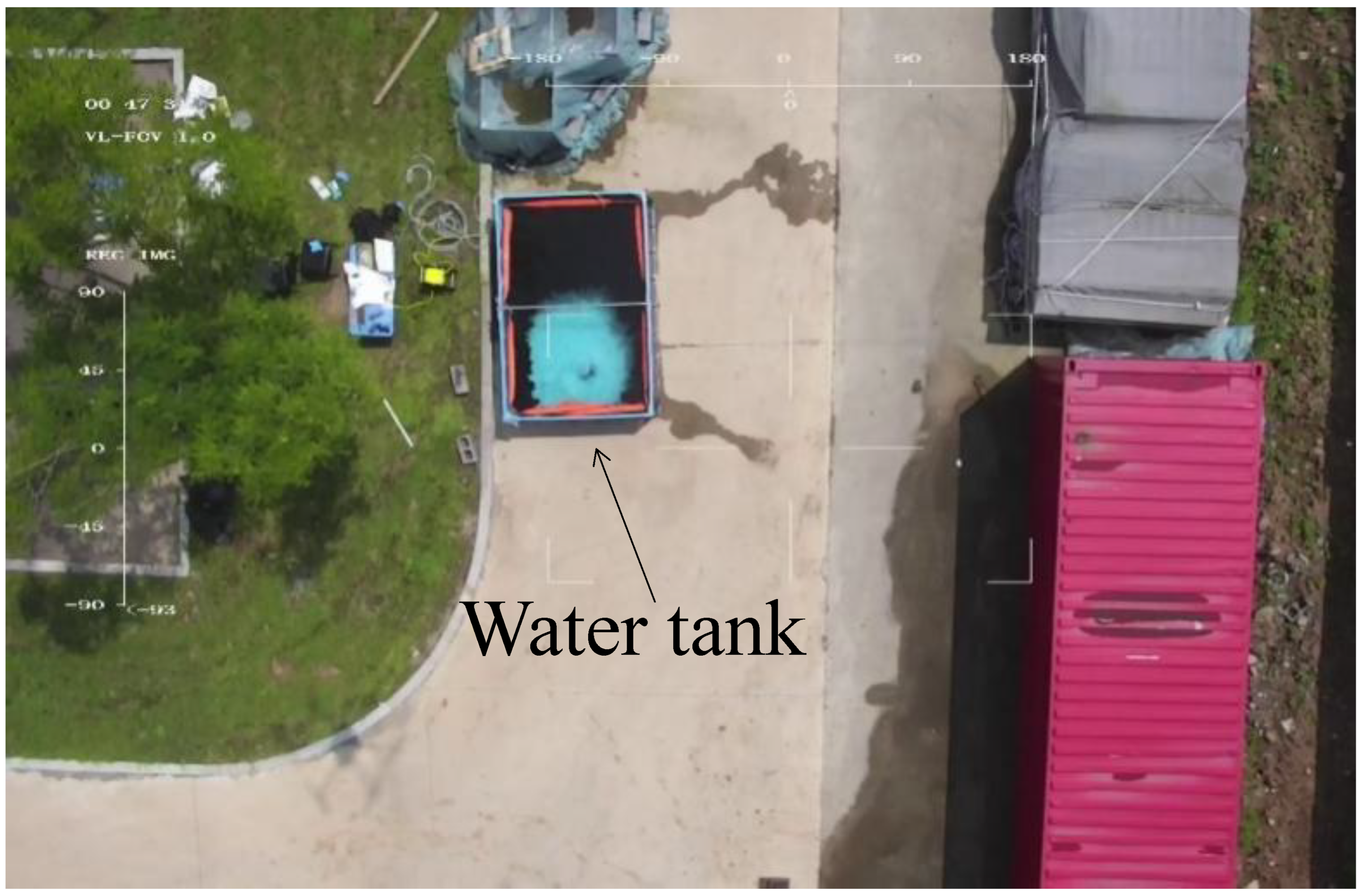
Figure 8 shows an RGB image of the experimental site. It can be seen that the image contains so many objects, including a water tank, green tress and lawn, a red big container and concrete pavements, etc., that it will increase the difficulty of calculating the oil slick area within the water tank.
A series of image processing procedures, including optical images extractions, oil slick target detection and oil slick area segmentation, was conducted to calculate the area of an oil slick. In order to remove color interference and extract the water tank from complex environments, the images were first converted from the RGB space into the HSV space. The spatial relationship between the target water tank and the background was accurately obtained based on the color constraint relationship between the target and the scene. The morphological processing, first including dilation and then erosion, was applied to improve the detection performance of the target water tank by repairing small defects and filling small cracks in images to capture target features based on the relationship between the scene and the target. The kernel sizes for the dilation and erosion were 5 × 5 pixels and 3 × 3 pixels, respectively. The position of the target water tank was successfully calibrated in the binary image after the morphological processing. Then, the contour of the target water tank was detected using the contour detection function. The coordinates of four vertices and the rotation center of the minimum circumscribed rectangle of the water tank were obtained to generate the rotation matrix.
Because the target water tank area only occupied about 0.08~0.58% of the entire image, the target water tank detection was defined as a small target detection task [
29]. To successfully detect the small targets, the water tank was considered to be an area of interest for ROI extraction. The water tank location in each image of the selected 1200 optical image dataset was cropped out using the ROI extraction algorithm. Then, the affine transformation function was used to correct the rotation of the image. The left image of
Figure 9 shows the cropped and corrected image of the water tank. It can be seen that the grayscale range of the oil slick area was very different from that of the clean water area. The RGB pixel values of the clean water area were much larger than the RGB pixel values of the oil slick area. Therefore, the oil slick area could be distinguished from the clean water area by properly setting the grayscale range.
A threshold segmentation algorithm was implemented to determine the oil slick area. The RGB thresholds (TR, TG, TB) were set as (60, 60, 60) based on the experimental observation. The pixels under the threshold were regarded as the oil slick area, while the pixels above the threshold were regarded as the background. The oil slick area was calculated by counting the number of the oil slick area pixels using Equation (2). To verify the threshold setting, a white square frame shown in
Figure 9 with an area of 370 mm × 440 mm was used for calibration. The area of the oil slick within the white frame was calculated to be around ~0.15 m
2. This was carried out by performing optical processing. The result was very close to the actual area of the oil slick of ~0.16 m
2 shown within the white frame. Then, the boomed area of the oil slick within the water tank was calculated with the same experimental setting. The right image of
Figure 9b shows the detected oil slick marked with yellow. It can be seen that the oil slick, including that outside of the boomed area, could be clearly identified except for the edges with much thinner oil, a result which indicates the correctness of the chosen RGB threshold values. The whole oil slick area within the water tank was calculated to be around ~2.33 m
2 when the pump was turned on.
5. Results
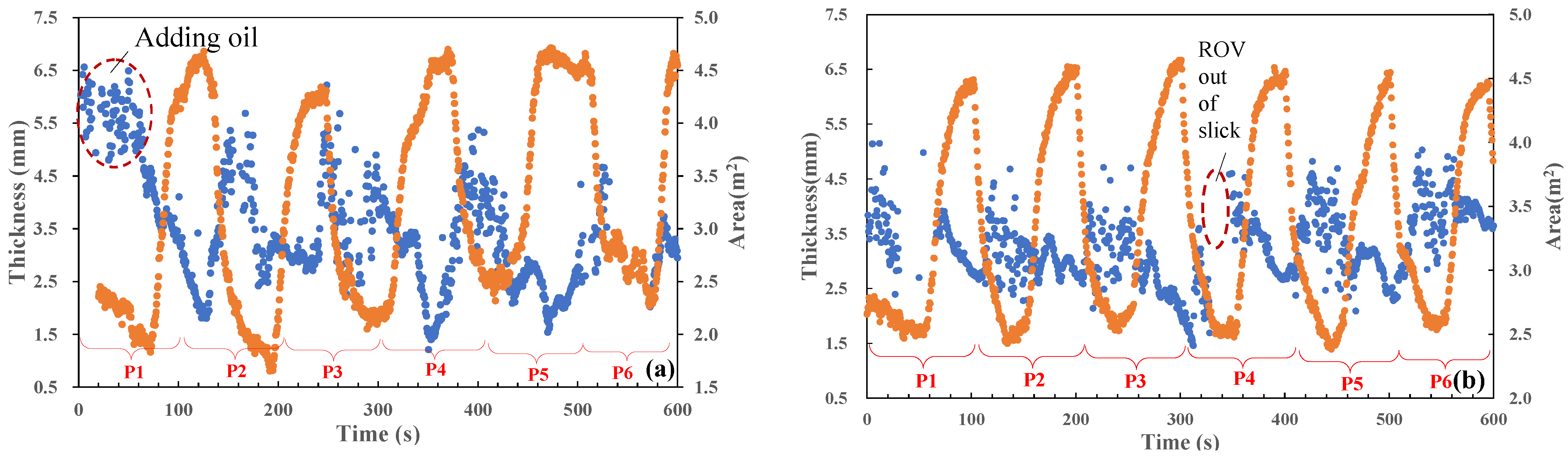
Figure 10a show the measurement of the thicknesses and areas of oil slick measured in test 1 with 10 L crude oil used. The thickness of oil slick was averaged over two channels. The blue and orange curves indicate the thickness and area of oil slick, respectively. We observed that the thickness outlined with a dashed red circle was a little higher at the beginning of the experiment when the crude oil was initially added in the boomed area. The thickness and area of the oil slick changed in the oppositely direction the pump was switched on/off. When the pump was powered on, the oil slick area quickly shrunk while the oil slick thickness increased.
Figure 10b shows the oil slick thickness and area measured in test 2. The oil slick thicknesses and area demonstrated similar changing trends as the test 1. The measured maximum and minimum areas of oil slick were nearly identical for each period, a result which indicates that the oil slick area measured with the optical image processing method had the high stability. The measured thickness dynamically shifted in the range of around 2.5 mm~4.5 mm in each period when the pump was turned on, a result which was mainly attributed to the continuously changing thickness caused by the surface water flow and the ROV’s continuous free movement. The thickness was not effectively measured at the time of around 350 s because the ROV was drifting out of the area of the oil slick.
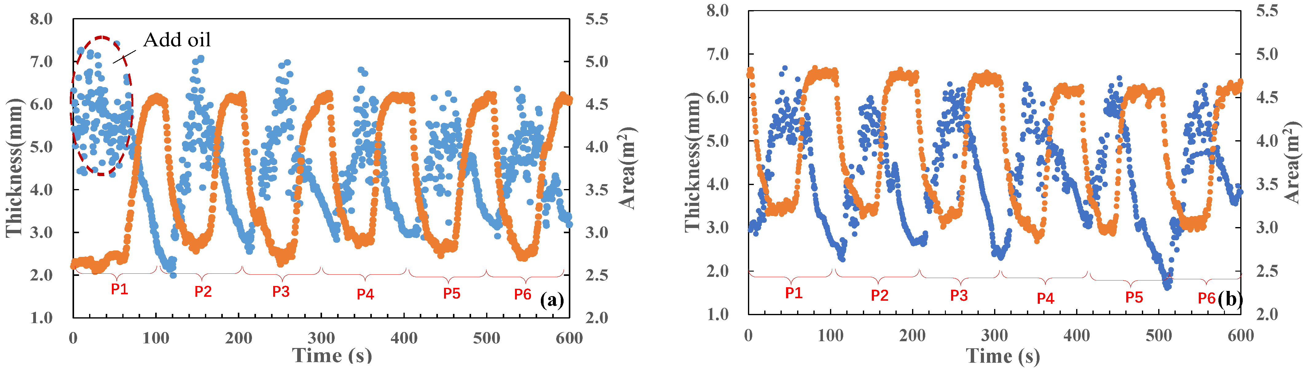
Figure 11a,b show the thickness and area measurements of the oil slick in two tests with 5 more liters of crude oil added in the boomed area. The measured area of the oil slick rarely changes while the measured thickness increases after adding 5 L more oil. When the pump was turned off, the thickness almost linearly decreased to the minimum thickness of around 2.0 mm~3.0 mm, while the area almost linearly rose to the maximum of around ~4.5 m
2. When the pump was turned on, the thickness was quickly driven by the surface water flow to dynamically rise to the maximum of 5.5 mm~7.0 mm, while the area shrunk to the minimum of around 2.7 m
2~3.0 m
2. The measured area and thickness of the oil slick showed similar trends for six periods, a result which further indicates the good repeatability and stability of this measurement technique.
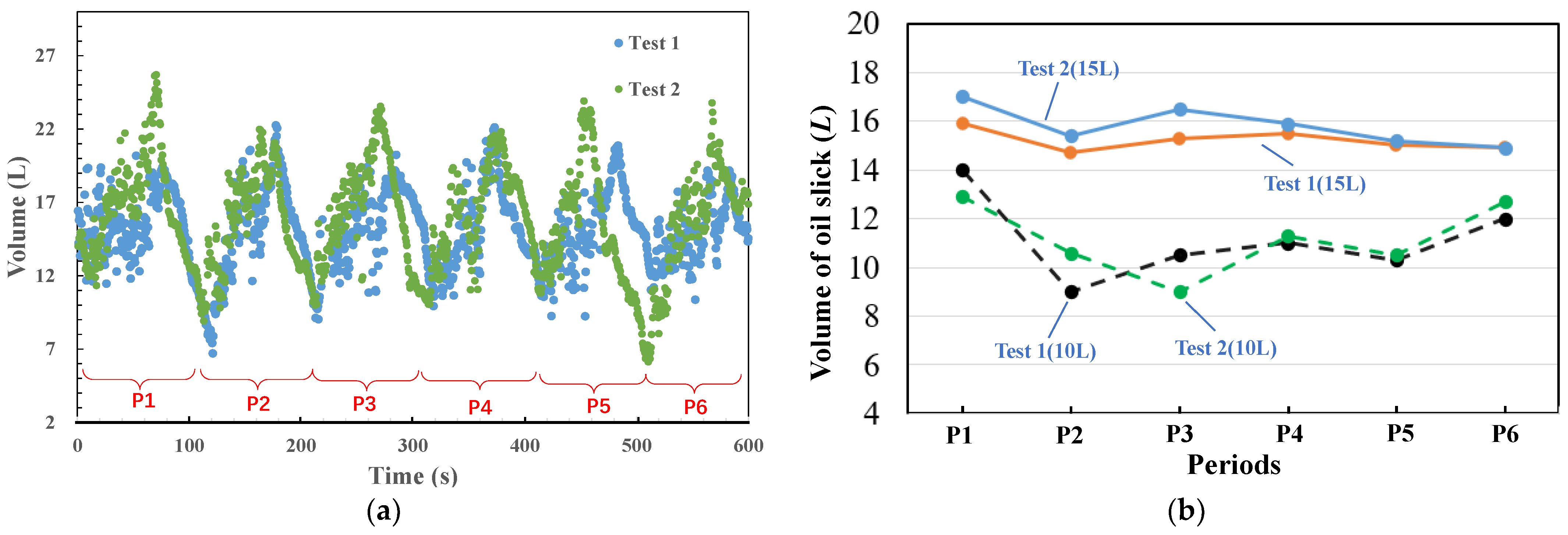
The volume of the oil slick was calculated by directly multiplying the measured thickness by the measured area.
Figure 12a shows the calculated oil slick volumes in two tests with 15 L crude oil applied. It can be observed that the volumes of oil slick were periodically fluctuating, with minima and maxima of around ~7 L and ~25 L, respectively, a result which may stem from the nonuniform thickness of the oil slick due to the surface water flow. In comparison to
Figure 11, it was found that the calculated volume of the oil slick was nearly synchronized with the measured thickness, a result which indicates that the oil slick volume measurement was more likely dependent on the oil slick thickness measurement. Since the oil slick thickness is usually nonuniform over the whole area and dynamically varies over time, implementing the local thickness measured at a specific time can result in some errors in the calculation of the oil slick volume. Therefore, developing the ultrasonic inspection system based on the ROV platform to image the distribution of the oil slick thickness will help to improve the measurement accuracy in the future.
In order to diminish the effects of the thickness on the measurement accuracy, the average of the oil slick volume was calculated within each period.
Figure 12b shows the volumes of oil slick averaged within each period. The average volumes of the oil slick measured in each period ranged from 9.0 L to 14.0 L, and 14.7 L to 17.0 L, with respect to 10 L and 15 L crude oil being added in the experiments, respectively. The average oil slick volume measured at the P1 period is usually a little higher than measurements in other periods due to the higher thickness measured at locations where oil is initially added.
Table 2 shows the average volume over each period, the volume averaged over 6 periods, and the standard deviation for each test. When 10 L oil was used, the oil slick volume averaged over 6 periods was around ~11.0 L for both tests, which was about 10% higher than the actually added volume of oil. After adding 5 L oil in the tank, the averaged oil slick volumes over 6 periods were around ~15.2 L, and ~15.8 L for two tests, which were roughly 1.3% and 5.3% higher than the actual volume of oil, respectively. The ratio of the standard deviation to the average volume was less than 15.0%, and 5.0% for the two measurements. The results demonstrate the relatively high measurement accuracy of the proposed method.
6. Discussion
In this article, a method is proposed that can be used measure the volume of oil slick by combining the measurements of the oil slick thickness and area using ultrasonic testing and image processing, respectively. A remotely operative vehicle (ROV) integrating two ultrasonic immersion transducers was deployed to measure the oil slick thickness boomed in a water tank. The collected ultrasonic signals were selected by abandoning distorted signals caused by the ROV’s movement and the surface water flow driven by a water pump. A cross-correlation algorithm was implemented to analyze selected ultrasonic signals to calculate the ultrasonic traveling time within an oil slick. The thickness of the oil slick was measured by multiplying the TOF by the speed of sound in oil. The measured oil slick thickness fluctuated due to surface water flow caused by a water pump.
Optical images of oil slicks were captured by a six-rotor drone which was remotely controlled to hover above the tank. The oil slick area was obtained by conducting optical image processing, including image preprocessing and image segmentation. For image preprocessing, the characteristics of an image were carefully analyzed, and then the most suitable algorithm was selected to detect the water tank area. Then, the water tank was cropped out with the appropriate algorithm. The best way of cropping the water tank area was to draw a rectangle based on the four vertices of the tank and utilize the rectangle to crop the image. However, due to the influences of light and the uneven colors of each area in the water tank, it was difficult to deploy the algorithm to accurately select four vertices of the water tank; these issues could result in some errors in the calculation.
The threshold segmentation algorithm was applied for image segmentation to determining the oil slick area in the water tank. The segmentation accuracy could be affected by the selected threshold values. Although the same experimental setting was implemented in the collection of optical image datasets at the same location, the acquired images could still be affected by the variation of light. When the image datasets were collected in conditions of low light, the RGB thresholds had to be increased. In addition, since the boundary between the oil slick and the water was irregular and fuzzy, the threshold was usually chosen within a certain range instead of a fixed value, which could potentially introduce some errors in the calculation of the oil slick area.
7. Conclusions
The thickness and area of the oil slick were successfully measured using the ultrasonic method and the optical image processing method, respectively. The cross-correlation algorithm was successfully used to process ultrasonic signals collected by ultrasonic transducers installed on an ROV. The image processing algorithm was implemented to calculate the area of the oil slick by analyzing optical image datasets captured by an optical camera of a 6-rotor drone. The accuracy of the oil slick area measurement was verified with the oil slick area within a frame. The volume of the oil slick was calculated by directly multiplying the thickness by the area of the oil slick. The calculated volume of oil slick was nearly synchronized in increasing/decreasing with the measured thickness when the pump was alternatively turned on/off, a result which implies that the volume measurement is more dependent on the thickness measurement than the area measurement. The average oil slick volume was less than 10% higher than that of the added oil, a result that demonstrates the high measurement accuracy of the proposed method. The proposed method has been experimentally verified for accurately measuring the thickness, area, and volume of oil slicks in laboratory experiments. It may be potentially used as a tool to collect information on oil spills including the thickness distribution, area, an volume, which can be helpful for designing the oil spill response strategy and evaluating the disposal efficiency in the oil spill field.
In the future, we will conduct more lab experiments to further validate the technical feasibility and accuracy of the proposed method in the oil spill response facility where real sea conditions can be simulated. In addition, we will integrate the ultrasonic inspection system on an autonomous underwater vehicle (AUV) platform to autonomously map the thickness distribution of oil slicks in the field. Furthermore, we will try to develop a cross-field platform that carries both ultrasonic inspection and optical systems to realize the measurements of the oil slick thickness and area.


