Article

Assessment and Projections of Marine Heatwaves in the Northwest Pacific Based on CMIP6 Models

1
School of Marine Sciences, Nanjing University of Information Science & Technology, Nanjing 210044, China
2
Southern Marine Science and Engineering Guangdong Laboratory (Zhuhai), Zhuhai 519000, China
3
Department of Oceanography and Coastal Sciences, Louisiana State University, Baton Rouge, LA 70803, USA
4
Center for Computation and Technology, Louisiana State University, Baton Rouge, LA 70803, USA
5
Coastal Studies Institute, Louisiana State University, Baton Rouge, LA 70803, USA
*
Author to whom correspondence should be addressed.
Remote Sens. 2023, 15(12), 2957; https://doi.org/10.3390/rs15122957
Submission received: 16 April 2023 / Revised: 26 May 2023 / Accepted: 3 June 2023 / Published: 6 June 2023

Abstract

:
To assess the abilities of global climate models (GCMs) on simulating the spatiotemporal distribution of marine heatwaves (MHWs), GCMs from the Coupled Model Intercomparison Program in Phase 6 (CMIP6) were evaluated from a historical period between 1985 and 2014 in the Northwest Pacific Ocean using a dataset that synthesizes remote sensing data. MHW simulation capabilities were assessed using Rank Score (RS) and Comprehensive Rating (MR) metrics that include both spatial and temporal scoring metrics. It was found that most CMIP6 models overestimate cumulative intensity, while mean and maximum intensities, in addition to the duration, were underestimated in the historical period. Possible future changes in MHWs were also examined based on the rank-based weighting ensembles under four shared socioeconomic pathways (SSPs) scenarios (SSP1-2.6, SSP2-4.5, SSP3-7.0, and SSP5-8.5). MHWs were identified using both a fixed 30-year baseline and a 30-year sliding baseline. In all scenarios, all MHWs metrics except frequency will have an increasing trend for the fixed baseline method. The frequency of MHWs will decrease after the 2050s. Days will first increase and then stabilize under various scenarios. MHWs will take place for more than 300 days by the end of the 21st century for the SSP5-8.5 scenario. The cumulative intensity in the SSP5-8.5 scenario is roughly six times higher than that in the SSP1-2.6 scenario by the end of the 21st century. A fixed baseline will result in near-permanent MHWs at the end of the 21st century. There will be no permanent MHWs at the end of the 21st century. Using the 30-year shifting baseline to define the MHWs can improve future MHW projections by capturing the spatiotemporal variability features of the MHWs.

1. Introduction

Marine heatwaves (MHWs) are events during which water temperatures are abnormally high and exceed the 90th climatological percentile for five or more consecutive days. [1]. They have strong influences on marine ecosystems [2], including temperature-sensitive coral reefs that often form the foundation for marine food chains and webs [3,4,5]. For example, MHWs are having an exacerbating impact on marine ecology in the Mediterranean Sea, posing an unprecedented threat to the health and functioning of ecosystems [6]. Marine animals such as Pacific cod are significantly impacted by MHWs in the Northeast Pacific, and the adverse effect of MHWs on fish supplies will double by 2050 [7].
As a global phenomenon, MHWs research is primarily focused on the Northeast Pacific [8,9,10], Indian [11,12], and Atlantic [13,14] Oceans. Additional research has also been conducted in the near-China seas [15,16,17], Bering Sea [18], Gulf of Alaska [19], Peruvian coastal waters [20], and northern and western oceans of Australia [21]. The Northwest Pacific is adjacent to the East Asian continent, and the interaction between the atmosphere and the ocean is significant. This region is particularly affected by the El Nino Southern Oscillation (ENSO) and Pacific Decadal Oscillation (PDO), and it is easily influenced by the anomalous Northwest Pacific Subtropical High (WPSH) and the anomalous anticyclone at a low level [22,23]. Under the control of the high-pressure system, there are more clear days, the wind speeds weaken, and the solar radiation increases, leading to an increase in the Sea Surface Temperature (SST), which can easily cause severe MHWs. The average frequency of MHWs in the Northwest Pacific Ocean from 1982 to 2016 was 2–3.5 times per year, with an average intensity of 2–5 °C [24]. During August 2016, the Yellow Sea experienced the most intense MHW on record since 1982 [25]. Record-breaking MHWs also occurred in the Northwest Pacific during the summer of 2020 [26]. Relatively fewer studies have been conducted on MHWs in the Northwest Pacific Ocean, and further research in this region is urgently needed.
The generation and evolution of MHWs are influenced by ocean dynamics, large-scale synoptic patterns, and teleconnection processes at various spatial and temporal scales [27,28,29]. These mechanisms include long-term anthropogenic climate warming [30], heat flux at the air–sea interface [31,32], atmospheric forcing [33], cloud feedback [34,35,36], ENSO [22,23,37,38,39], PDO [9], Madden–Julian Oscillation (MJO) [13,25,40], and the WPSH [25,26]. In contrast to atmospheric forcing, Wang et al. [41] pointed out that oceanic dynamics can help to explain the increasing trend of marine heatwaves, which may increase the surface latent heat flux. According to Barkhordarian et al. [42], due to the recent decrease in the industrial aerosol load and the elevated levels of greenhouse gases, MHWs are situated next to a systematically forced outstanding warming pool in the Northeast Pacific. The ENSO plays a considerable role in influencing the concurrence of MHWs in the Northwest Pacific region. According to Liu et al. [22] and Tan et al. [23], an El Niño event would lead to an anomalous anticyclone over the Northwest Pacific, which is a prime system affecting the East Asian monsoon. The anomalous anticyclone will lead to a weakening of northeasterly winds in autumn, which in turn would lead to less ocean heat loss. An anomalous anticyclone can also increase the shortwave radiation, causing the South China Sea to warm. A significant warming of the surface layer results from reduced mixing in the upper ocean, caused by stronger solar radiation and weaker wind speeds. The MJO caused more tropical cyclones, which are important factors in the occurrence of extreme MHWs in the Yellow Sea [25]. The WPSH is considered to be the primary anticyclone system for the climate variability in the Northwest Pacific. The splitting of the WPSH into two independent components of eastern and western segments promoted the formation and development of the MHW in the Yellow Sea in August 2016. There are significant regional differences in the occurrence mechanism of marine heatwaves, which are controlled by local processes and large-scale circulation fields, and the physical mechanism is relatively complex, which requires a concrete analysis of a particular MHW event.
During the last century, MHWs have been intensifying, occurring more frequently, and lasting longer. Their intensity, frequency, and duration will continue to increase with global warming [2,43,44,45]. An effective tool for projecting changes in MHW events in the future is a climate model. Pilo et al. [46] suggested that high- and medium-resolution models were more effective at simulating the spatial distribution of MHWs, but there is still significant variability among the models. This was attributed to an underestimation of SSTs in eddy-rich regions in lower-resolution models. By comparing the capabilities of 19 models from the Coupled Model Intercomparison Project Phase 5 (CMIP5) and 29 models from the Coupled Model Intercomparison Project Phase 6 (CMIP6) to simulate MHWs, Qiu et al. [47] demonstrated that the CMIP6 model had better simulation results than CMIP5 in most regions, and the deviations in the intensity and duration of simulated CMIP6 model MHWs were within 0.5 °C and 10 days, respectively. It was also suggested that MHWs will become more intense and prolonged in the 2070s under the SSP5-8.5 scenario of the shared socioeconomic pathways (SSPs) [48].
Current research on MHWs in the northwestern Pacific Ocean mainly focuses on its temporal and spatial variation characteristics [41], the physical mechanism for specific MHW events [17,49], and its effects on ecosystems [4]. The previous studies for this region [27,29,47,50] just evaluated either CMIP5 or CMIP6 based on spatial and temporal skill scores, respectively. In addition, those studies merely used the mean intensity, duration, and total days to describe the features of MHWs. There are still significant uncertainties in model projections, which may be caused by model uncertainty, random intrinsic variability in the climate system itself, and scenario uncertainty. The multi-model ensemble (MME) method is used in future climate projections to increase the level of reliability. The majority of the studies mentioned above followed a simple MME method in which each model contributing to the future projection of MHWs was given equal weight [51]. To overcome these limitations, this study used six metrics of MHWs, as well as CMIP6 data from four emission scenarios. Future projections of MHWs in the Northwest Pacific Ocean (90°E-160°E and 0–60°N) were conducted using MME and a rank-based weighting approach. The weight of each CMIP6 model was calculated by its historical simulation skill. The Comprehensive Rating (MR) metrics, which are used to determine a comprehensive ranking for each model, were calculated in order to quantify each model’s capacity. The weighted ensembles were then used for future projections.
The remainder of this paper is organized sequentially as follows. Section 2 describes the data and methodology used in this study. The spatiotemporal characteristics of past and future MHWs are provided in Section 3, along with the capabilities of CMIP6 models to simulate MHWs. Finally, Section 4 summarizes our results and outlines potential directions for future research.

2. Data and Methodology

2.1. Data

2.1.1. Observed Sea Surface Temperature

SST data were from the Optimal Interpolation Sea Surface Temperature (OISST) Dataset of the National Oceanic and Atmospheric Administration (NOAA) [52], which is one of the most advanced SST products, with a spatial resolution of 1/4° × 1/4° and a time range of 1981 to the present. It is widely used for climate monitoring and model validation and is produced using a variety of sources, including remote sensing SST data from the Advanced Microwave Scanning Radiometer (AMSR) and the Advanced Very-High-Resolution Radiometer (AVHRR), in situ data from ships and buoys, and sea ice data. The production and maintenance of the product take place with a 1-day delay. The data are available at https://www.ncei.noaa.gov/products/optimum-interpolation-sst (accessed on 25 May 2023). This product was utilized for assessing the performances of the CMIP6 models during the historical period (1985–2014).

2.1.2. Simulated SST by CMIP6 Models

The SST field by 16 CMIP6 models from 11 different institutions in 8 countries/regions with resolutions ranging from 25 to 250 km was also used for this study (Table 1). To assess the model’s performance, daily SST fields (variable name: tos) from native model grids (grid label: gn) were analyzed under the historical experiments. To project future MHWs, four scenario datasets from the Scenario Model Intercomparison Project (ScenarioMIP) were also used: SSP1-2.6, SSP2-4.5, SSP3-7.0, and SSP5-8.5 [48]. The four different types of SSP scenario data correspond to low, medium, and high radiation and high radiation forcing, respectively. SSP1-2.6 emphasizes more inclusive development that respects the perceived environmental limitations and chooses the green route with sustainable settings. The radiation forcing will stabilize at around 2.6 W/m2 in 2100 after peaking at 3.1 W/m2 in the middle of the 21st century. SSP2-4.5 is seen as a “middle road”, combining the medium-term population increase, emissions, and problems of mitigation and adaptation. By 2100, the radiation forcing will stabilize at around 4.5 W/m2. SSP3-7.0, stabilizing at 7.0 W/m2 in 2100, combines the relatively high societal vulnerability and radiation forcing. SSP5-8.5 is a “fossil fuel development” pathway. The radiation forcing will be essentially stable at 8.5 W/m2 in 2100. The data are available at https://esgf-node.llnl.gov/projects/cmip6 (accessed on 25 May 2023). All data were regridded and bilinearly interpolated to a common grid with a spatial resolution of 1°.

2.2. Methodology

2.2.1. Marine Heatwave Detection

The definition of MHWs promoted by Hobday et al. [1] was used in this study to calculate statistics for MHWs at each grid point. An MHW event is one where the daily average SST for a grid point exceeds the 90th percentile (threshold) of the 30-year historical base period (1985–2014) for at least five consecutive days. It is considered to be an MHW event if there are fewer than or equal to two days between two MHW events. Due to the unequal resolution, OISST and CMIP6 model data were regridded and bilinearly interpolated to a common grid with a spatial resolution of 1°. The average climate state and threshold for MHW events were computed using OISST and CMIP6 historical scenario data from 1985 to 2014. Following that, distinctive statistics for each year’s MHW events were detected.
However, there is no consensus on which baseline should be utilized to calculate the SST anomalies. Many of the current studies appear to support the use of a 30-year fixed baseline [1,53]. The fixed baseline approach fails to consider the fact that the oceans are gradually warming due to the effects of climate change, which will result in the increasing duration of the MHW, and even a year-round persistent ocean heat wave event at the end of the 21st century. In order to solve this problem, many scholars have proposed the use of shifting reference climate states to study MHWs [54]. Therefore, we also used a 30-year running-mean baseline to identify MHWs. These metrics included the average intensity (MeanInt), the maximum intensity (MaxInt), the cumulative intensity (CumInt), the mean frequency (Frequency), the duration (Duration), and the number of days (Days).
There is a significant bias in the SST simulated by the climate model [55], which is bound to affect the detection results of MHWs. We have employed the quantile mapping method [56] to adjust the bias of the CMIP6 models. This approach involves quantifying the bias for each percentile in the cumulative distribution function of the historical simulation and then incorporating it into future simulations. To maintain the recommended 30-year climatology for detecting MHWs, only the initial three years (1982–1984) were utilized for data calibration. As a result, the historical results are limited to the period of 1985–2014.

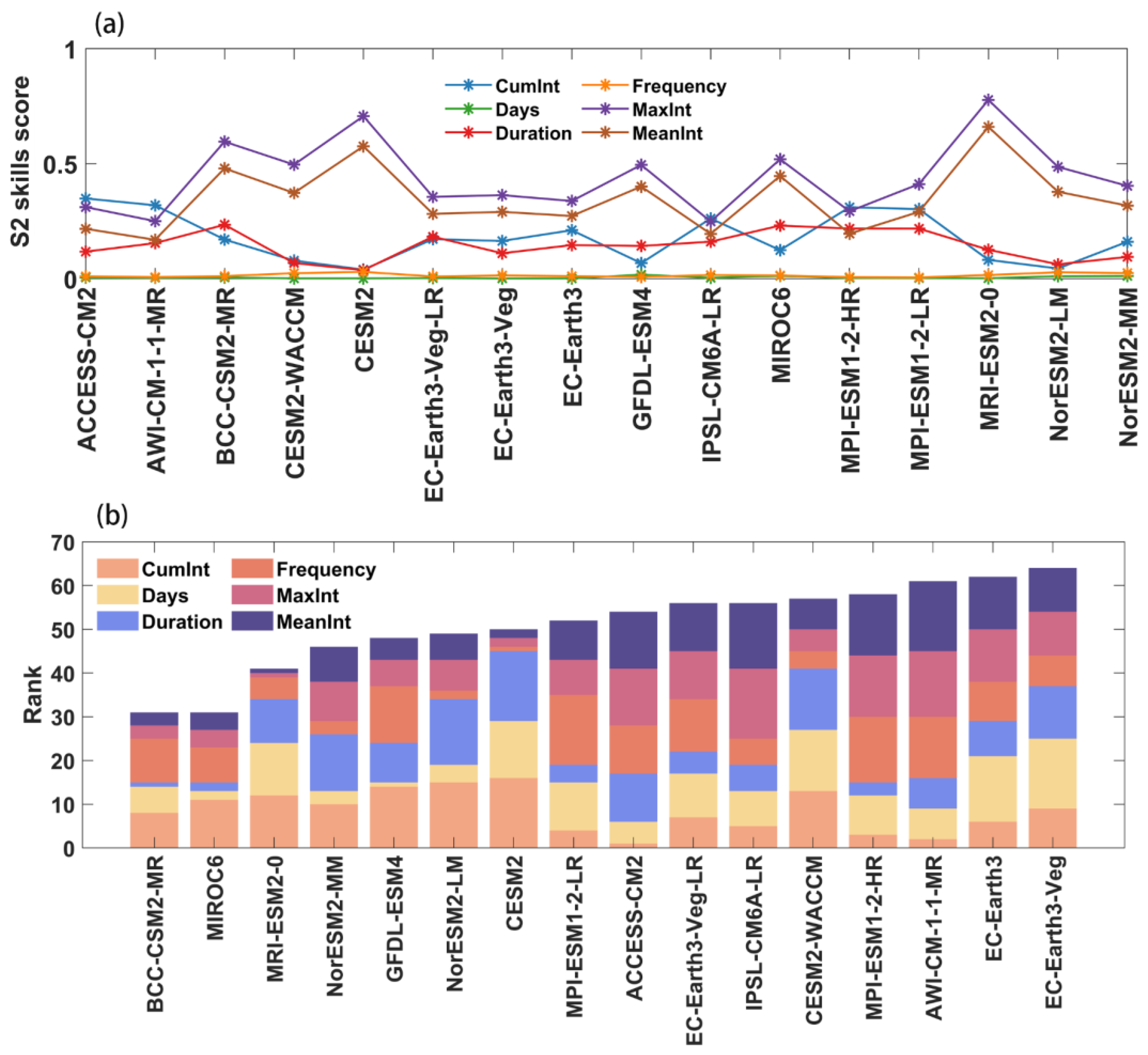
2.2.2. Spatial Skill Scoring Metric

The CMIP6 model’s simulation of MHWs was assessed using the Taylor diagram [57] in this study. Using the triangulation of the correlation coefficient (R), the root mean square deviation (RMSD), and the standard deviation (STD) between two fields or two series, Taylor diagrams present all three on the same figure at the same time. The correlation coefficient (R) indicates the similarity of the spatial distribution between the model simulation results and observations (OISST), the standard deviation (STD) indicates the dispersion of the data itself, and the root mean square deviation (RMSD) indicates the deviation between the model results and observations. A Taylor diagram allows for a visual comparison of the strength of each model’s simulation capability.
In order to better assess the capability of the model simulation, this study introduced two evaluation metrics (S1 and S2) to quantify the correlation coefficient and standard deviation between the simulated and observed fields. They are defined as
S 1 = 4 ( 1 + R ) ( σ f + 1 / σ f ) 2 ( 1 + R 0 ) ,
S 2 = 4 ( 1 + R ) 4 ( σ f + 1 / σ f ) 2 ( 1 + R 0 ) 4 ,
where R is the correlation between the observation and the model, where R0 is the highest correlation coefficient, and σf is the ratio of the standard deviation of the simulation to the standard deviation of the observation. The closer the model is to the observation, the closer the value of S is to 1, and the greater the model’s capacity for simulation. S tends to 0 when the correlation coefficient is less or when the model standard deviation ratio is infinite. The main difference between the two indicators is that S2 gives more weight to taking the correlation coefficient into account.

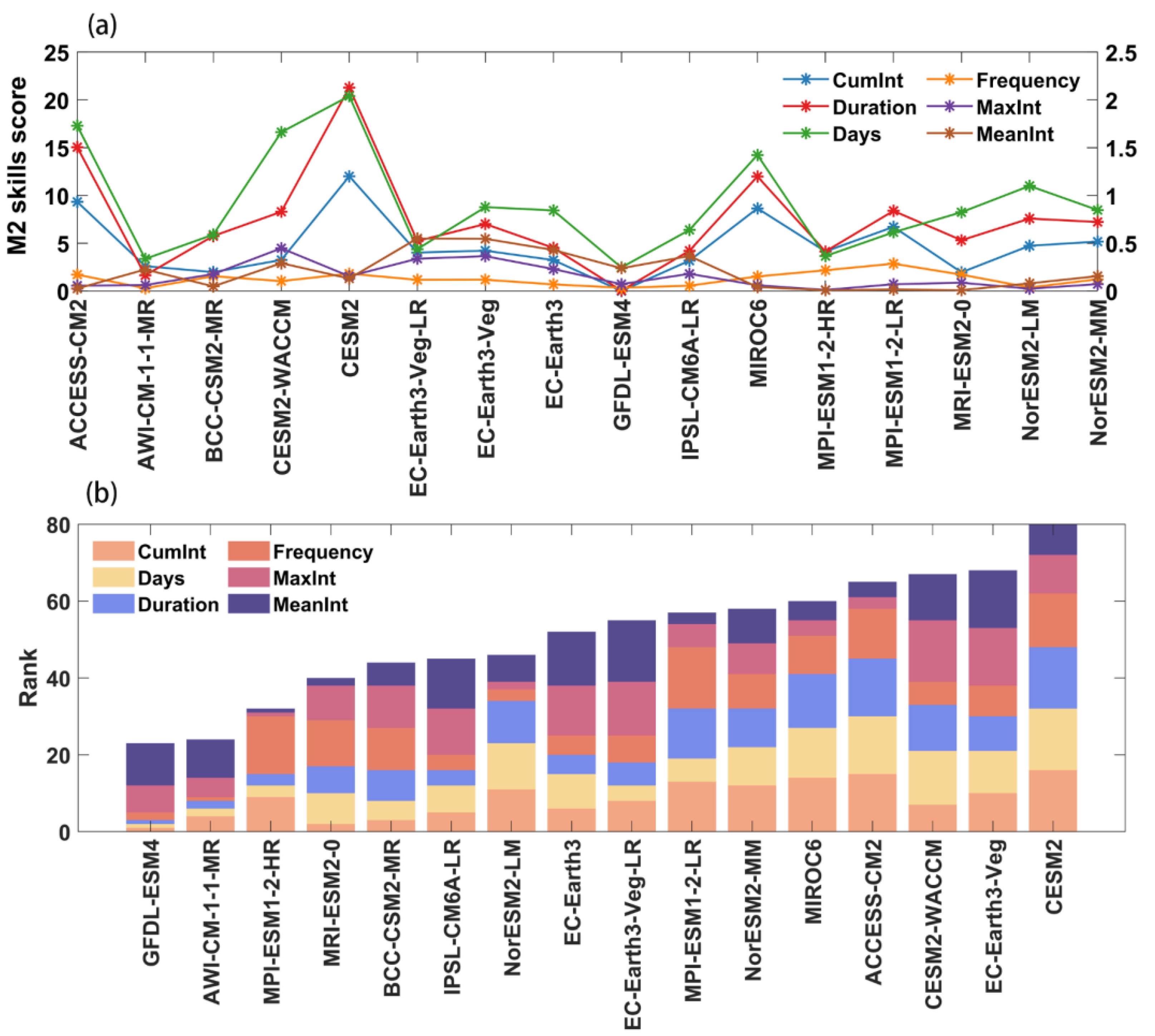
2.2.3. Temporal Skill Scoring Metric

This study used the temporal skill score M2 [58] to assess how well each model can simulate the interannual variability in relation to the observed time series. M2 is defined as follows:
M 2 = ( S T D m S T D o S T D o S T D m ) 2 ,
where STDm denotes the standard deviation of the time series at each point in the model field, and STDo denotes the standard deviation of the time series at each point in the observation. When STDm and STDo are the same, the M2 is equal to 0. Lower M2 values indicate a stronger agreement between observations and simulations.

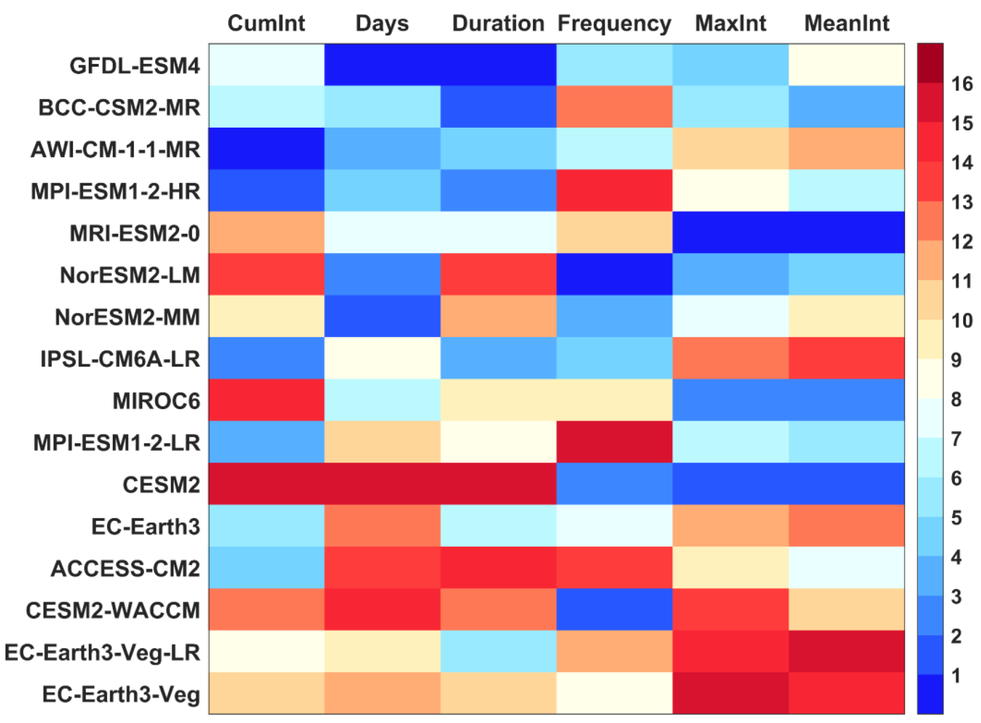
2.2.4. Rank Score Method

The RS method was used in order to combine the spatial skill score S with the temporal skill score M2 [59]. This method can comprehensively evaluate the simulation capability of the model by using different evaluation criteria, which are defined as
R S i = { 1 T i T m i n T m a x T m i n , T   i s   r e l a t i v e   e r r o r   e v a l u t i o n   i n d i c a t o r T i T m i n T m a x T m i n , T   i s   n o n r e l a t i v e   e r r o r   e v a l u t i o n   i n d i c a t o r ,
where RSi represents the score of the ith model, Ti represents the indicator value calculated by the ith model, and Tmax and Tmin represent the maximum and minimum values of the indicators, respectively, where the relative error evaluation indicator corresponds to the M2, and the non-relative error evaluation indicator relates to the S1 and S2. Scores lower than 1 and a higher RS score are preferable. The evaluation score was weighted to produce the final score. M2 was given a weight of 1.0, and S1 and S2, which are different indications with the same skill score, were each given a weight of 0.5. The performance of the model simulation improves with a higher overall score.

2.2.5. MR Composite Metrics

This study also introduced the MR comprehensive indicator [60,61] to comprehensively evaluate six MHW metrics and completely rank each model so as to assess the comprehensive simulation capabilities of each model for multiple MHW metrics. It is defined as:
M R = 1 1 ( 1 × n × m ) i = 1 n r a n k i ,
where n is the total number of indicators used in the assessment, m is the total number of models, and ranki is the ranking of each model with respect to a different assessment indicator. For the model with the best simulation ability, ranki is equal to 1. The more closely the MR approaches 1, the better the model’s capacity for simulation.

2.2.6. Weighting Methods

Different weights were assigned to the model to assess the change in the MHW based on the ranking of each model’s comprehensive simulation capacity of the spatial and temporal simulation ability [58]:
R i = i = 1 N S i S i ,
where Ri is the weight quality index (the larger the value is, the better the effect of the model simulation) and Si is the rank of the model calculated by the MR method (the smaller the rank is, the greater the weight of the model). After normalization, the weights accounted for by each model can be obtained as follows:
W i = R i i 1 N R i ,
where Wi is the weight of each mode, and N is the total number of models.

3. Results

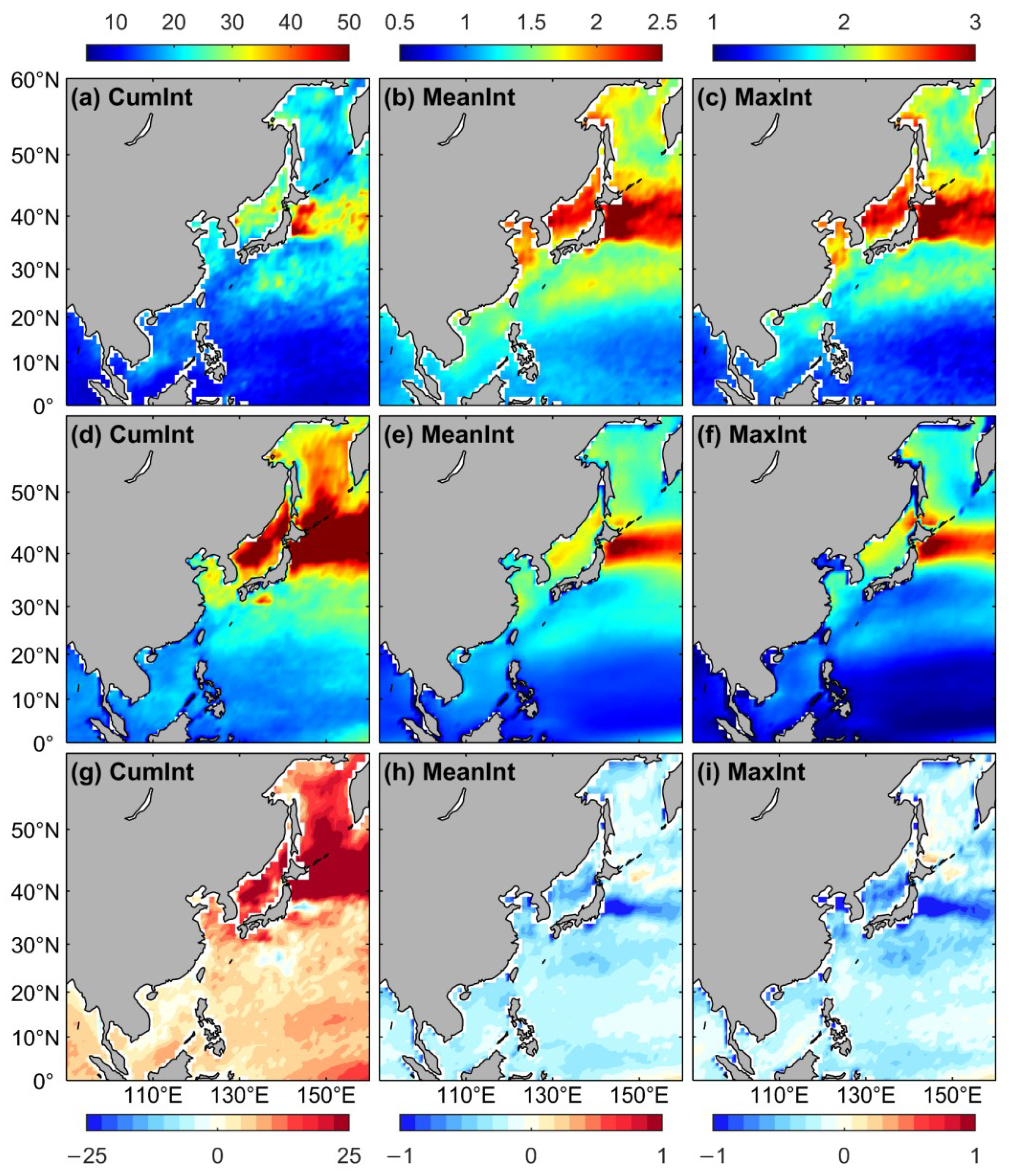
3.1. Marine Heat Waves during the Historical Period (1985–2014)

Taylor diagrams were used to evaluate how well models reproduce the spatial pattern of a variable. The Taylor diagram of the CMIP6 model simulations against OISST is shown in Figure 1. Most CMIP6 models reproduce MHW intensity (MeanInt, MaxInt, and CumInt) reasonably well (Figure 1a–c). The correlation coefficients reach the maximum values of 0.8957, 0.8937, and 0.7457, respectively. However, the simulation of Frequency, Duration, and Days by CMIP6 models is much poorer and their average correlation (R) is 0.1893, 0.1753, and -0.1706, respectively. There is a negative correlation for Duration and Days, respectively. For MeanInt, the R is between 0.6882 and 0.8957, the STD is from 0.7342 to 1.8466, and the RMSD is between 0.4586 and 1.0768. The simulation result of MaxInt is very similar to that of MeanInt, and the capabilities of the models do not differ significantly from one another. The RMSD ranges from 0.459 to 1.0046, the R ranges from 0.6746 to 0.8937, and the STD is between 0.7224 and 1.777. In general, there is neither a particularly strong nor a particularly weak model. For CumInt, the correlation of the majority of model results hovers around 0.6, and the spatial R of two of the models is greater than 0.7. The MRI-ESM2-0 model provides better simulation results for MHW intensity (MeanInt, MaxInt, and CumInt). The R for most Frequency (Figure 1d) simulation results is not particularly good, suggesting that most models have a poor capacity, with NorESM2-LM having the highest R at 0.3195. For the simulation of Duration (Figure 1e), MPI-ESM1-2-LR is the best in terms of correlation; however, the value of the correlation is only 0.4182. Other models have much lower Rs or even negative Rs. It is clear that the CMIP6 models’ capacity to simulate Duration is relatively poor. For Days, the CMIP6 models have the worst simulation performance (Figure 1f). The best model, GFDL-ESM4, has an R of 0.136, and the correlation coefficients are around −0.4–0.1 for most CMIP6 models. Twelve out of the sixteen models have inverse Rs. The STD and RMSD are also much larger than 0.5 and 1. The results show the unreliability of the CMIP6 models’ simulation of MHW Days for the studied region.
The S1 skill scores of the CMIP6 model for the six MHW metrics (CumInt, Days, Duration, Frequency, MaxInt, and MeanInt) are displayed in Figure 2a. The models have an S1 value ranging from 0.3824 to 0.6268 and a mean value of 0.5423. The Duration of MHWs is the best. The models perform the worst in reproducing the Days of MHWs, with an S1 value ranging from 0.0362 to 0.0814 and a mean value of 0.0512. The mean S1 spatial skill scores for MaxInt, MeanInt, CumInt, and Frequency are 0.5065, 0.4006, 0.2988, and 0.0591, respectively. The results imply that there are significant disparities among the various models’ spatial modeling capabilities for MHWs. IPSL-CM6A-LR, with an S1 value of 0.6268, has the best capacity to model Duration. For the simulation of MaxInt, MeanInt, and Frequency, the performance of CESM2 is the best, with S1 values of 0.8024, 0.6771, and 0.1059, respectively. ACCESS-CM2 has the best ability to simulate CumInt, with an S1 value of 0.6816, and GFDL-ESM4 has the best ability to simulate Days, with an S1 value of 0.0814. The cumulative ranking of the S1 skill scores for each model in simulating the characteristics of MHWs is shown in Figure 2b. The top two models are MIROC6 and MRI-ESM2-0, indicating that these two models have the best capability of spatial simulation. EC-Earth-Veg, AWI-CM-1-1-MR, and EC-Earth3 have the weakest spatial ability to simulate MHWs in the studied region.
Figure 3 shows the S2 skill scores of CMIP6 models and their cumulative ranking. Most CMIP6 models have the best spatial simulation capabilities for MaxInt. The S2 values for MaxInt range from 0.2487 to 0.7775 with an average of 0.4408 (Figure 3a). The models have the worst spatial simulation capability for Days. The S2 values range from 0.0012 to 0.0175, with an average of 0.0055. The average S2 values for MeanInt, CumInt, Duration, and Frequency are 0.3466, 0.1786, 0.1441, and 0.0148, respectively. MRI-ESM2-0 shows the best skills in simulating MaxInt and MeanInt, with S2 values of 0.7775 and 0.6602, respectively. The model that best simulates CumInt is ACCESS-CM2, with an S2 of 0.3490. The model that shows the best skill in simulating Duration is BCC-CSM2-MR, with an S2 value of 0.2346. CESM2 shows the best skill in simulating Frequency, with an S2 value of 0.0297. The model that best simulates Days is GFDL-ESM4, with an S2 value of 0. Overall, the two best models for simulating MHWs in the Northwest Pacific Ocean are BCC-CSM2-MR and MIROC6. AWI-CM-1-1-MR, EC-Earth3, and EC-Earth3-Veg have the worst ability to simulate MHWs in the region (Figure 3b).
Considering both the S1 and S2 scores, the majority of the chosen CMIP6 models can effectively simulate MaxInt and MeanInt, followed by simulations of CumInt. The models show less of an ability to simulate Frequency and Days. The assessment approach has an impact on how well Duration can be simulated. BCC-CSM2-MR, which ranks third overall in the S1 method, ranks first in the S2 method that focuses on the spatial R. Therefore, the selection of various evaluation methods of S1 and S2 can comprehensively evaluate the model simulation ability and reduce the effect of method errors. Overall, BCC-CSM2-MR, MIROC6, and MRI-ESM2-0 are the models with a good comprehensive capacity for the spatial simulation of MHWs based on the six metrics, while AWI-CM-1-1-MR, EC-Earth3-Veg, and EC-Earth3 are the models with a relatively weak comprehensive capacity for the spatial simulation of MHWs.
Using the M2 time skill score, the ability of the CMIP6 models to simulate the interannual variability in MHWs was assessed as well (Figure 4). Figure 4a shows that the CMIP6 models have the highest ability to simulate the temporal variability in Frequency relative to the other MHW metrics, with M2 values ranging from 0.0285 to 0.2860 and a mean value of 0.1264. The simulation ability of Duration is the worst, with a mean M2 value of 7.3547 and values ranging from 0.0389 to 21.2906. MaxInt, MeanInt, Days, and CumInt have mean values of 0.1505, 0.1977, 0.9113, and 4.6997, respectively. The model that best simulates Frequency is AWI-CM-1-1-MR, with an M2 of 0.0284. The MPI-ESM1-2-HR model exhibits the best simulation accuracy for MaxInt and MeanInt, with M2 values of 0.0112 and 0.0077, respectively. The model that best simulates Days, CumInt, and Duration is GFDL-ESM4, with M2 values of 0.2462, 5.5753 × 10⁻⁷, and 0.0389, respectively. Figure 4b shows that GFDL-ESM4 and AWI-CM-1-1-MR are the best at simulating the temporal variability in MHWs. The simulation abilities of the MHW’s temporal variability in the region are relatively weak for the CESM2, EC-Earth3-Veg, and CESM2-WACCM models.
Using the RS approach (Table 2), AWI-CM-1-1-MR, MPI-ESM1-2-HR, IPSL-CM6A-LR, MPI-ESM1-2-LR, ACCESS-CM2, and EC-Earth3 are the models that best simulate CumInt. Considering both the M2 temporal skill score and the S spatial skill score, the model AWI-CM-1-1-MR shows the best skills in temporal and spatial simulation. CESM2 has the lowest overall ranking for both the S2 and M2 skill scores. For the simulation of Days, the six best models are GFDL-ESM4, NorESM2-MM, NorESM2-LM, AWI-CM-1-1-MR, MPI-ESM1-2-HR, and BCC-CSM2-MR. Among all models, GFDL-ESM4 has the best spatial simulation capabilities. Although the CESM2 model is not the least skillful in terms of the spatial skill score, it is the poorest in the overall RS ranking because of the low temporal skill score. GFDL-ESM4, NorESM2-MM, NorESM2-LM, AWI-CM-1-1-MR, MPI-ESM1-2-HR, and BCC-CSM2-MR are the top six models for the simulation of Duration. The top six models for the simulation of Frequency are NorESM2-LM, CESM2-WACCM, CESM2, NorESM2-MM, IPSL-CM6A-LR, and GFDL-ESM4. Despite not having the best spatial and temporal simulation capabilities, NorESM2-LM comes in first overall. The MPI-ESM1-2-LR model has the lowest overall ranking and the worst S and M2 indication rankings, with an RS of 0. For MaxInt, the top six models are MRI-ESM2-0, CESM2, MIROC6, NorESM2-LM, GFDL-ESM4, and BCC-CSM2-MR. MRI-ESM2-0 ranks first overall and has outstanding spatial simulation capabilities, but it is not the best in terms of temporal simulation capabilities. EC-Earth3-Veg has the worst overall ranking, with the lowest S1, S2, and M2 skill scores. The top six models for the simulation of MeanInt are MRI-ESM2-0, CESM2, MIROC6, BCC-CSM2-MR, NorESM2-LM, and MPI-ESM1-2-LR, of which the three best models are the same as those for the simulation of MaxInt. The MRI-ESM2-0 model has excellent spatial simulation capability. It comes in second for the M2 skill score but comes in first overall. The EC-Earth3-Veg-LR model comes in last with the lowest simulation capability.
The comprehensive simulation capabilities of the CMIP6 model were assessed using the RS ranking of the six MHW metrics through the comprehensive rating metric MR (Figure 5). The capabilities of the models were ranked from top to bottom by model rank, with smaller numbers (blue) indicating a more reliable model. It can be seen that the top three models based on the MR are GFDL-ESM4, BCC-CSM2-MR, and AWI-CM-1-1-MR. Their relative resolutions are 50 km, 100 km, and 25 km, respectively. The least skillful models are EC-Earth3-Veg, EC-Earth3-Veg-LR, and CESM2-WACCM, all of which have a resolution of 100 km. The resolution of these three models is not the lowest among all CMIP6 models. Although there is not an exact positive correlation between resolution and model performance in the simulation of MHWs, high-resolution models are generally better at simulating MHWs overall, which is consistent with the conclusion by Qiu et al. [47].
The mean distribution of the six MHW metrics obtained from CMIP6 models and OISST data and the differences between them during the historical period are shown in Figure 6 and Figure 7. The overall MHW features in CMIP6 models are largely similar to those in OISST. Over most of the study area, the simulated Frequency, MeanInt, and MaxInt of MHWs by CMIP6 models are smaller than those of OISST data. The negative biases are mainly at the Kuroshio Extension Region (KER) for Frequency, while there are positive biases in the northern part of the KER for the simulated MeanInt and MaxInt. The simulated CumInt, Days, and Duration of MHWs by the CMIP6 model are higher than those detected using the OISST data. The positive biases for the simulated CumInt and Duration are mostly at the KER and to the north of it. The positive bias for the simulated Days is located to the south of 20°N, while the negative bias is primarily situated to the east of the Japanese archipelago.
The time series of the six MHW metrics in the CMIP6 model and OISST data during the historical period for the Northwest Pacific are shown in Figure 8. During the three decades (1985–2014), the frequency of MHWs is increasing at a rate of 0.89 times/decade, while the MeanInt is increasing at a rate of 0.01 °C/decade, and the Duration of MHWs is increasing at a rate of 1.36 days/decade. The metrics MaxInt, CumInt, and Days for MHWs also show an increase of approximately 0.02 °C/decade, 4.2 °C/decade, and 18.42 days/decade, respectively. Compared with the OISST data, the CMIP6 models show a larger CumInt and Duration, but a smaller MeanInt and MaxInt. The simulated Frequency and Days are similar. The mean intensity of MHWs fluctuated throughout the 1990s, but there was a slight upward trend. The Frequency, Duration, and Days varied significantly at the end of the 1990s. The choice of the baseline period (climatology) should be related to this intensity or the overall increasing trend. As in previous studies [44,47,50], the mean intensity of MHWs detected in the CMIP6 model was much weaker but their duration was longer [47]. This may be primarily because most models overestimate SST anomalies by small-scale processes and the simulated SST is excessively smooth [44,50].

3.2. Projections of Marine Heatwaves in the 21st Century

3.2.1. Results for the Fixed Baseline

The mean distribution of the MHW Frequency based on the fixed baseline throughout the 21st century is shown in Figure 9. MHWs will occur more frequently in the southern part of the Northwest Pacific region and less frequently in the northern part in the 21st century. The Frequency in the majority of the Northwest Pacific is expected to increase significantly from 1.2794 during the early part of the 21st century (2015–2040) to 2.6727 by the middle of the 21st century (2041–2070). The Okhotsk Sea, the South China Sea, and the eastern part of the Philippines will experience the most significant increase in Frequency. In most of the Northwest Pacific, MHWs will be less frequent at the end of the 21st century (2071–2100) compared with the middle period (2041–2070). The decrease in Frequency is most noticeable in the Kuroshio Extension Region. The simulated Frequency also differs among different emission scenarios. In the early part of the 21st century, there will be the highest mean Frequency in the Northwest Pacific for the SSP1-2.6 scenario, followed by the SSP2-4.5 and SSP3-7.0 scenarios, while it will be the lowest for the high-emission SSP5-8.5 scenario, with values of 1.33, 1.3183, 1.2628, and 1.2066, respectively. The difference in the simulated Frequency among the different emission scenarios is regionally dependent. For example, the Frequency in the Okhotsk Sea will be larger in the SSP2-4.5 (Figure 9d) and SSP3-7.0 (Figure 9g) scenarios than in the SSP1-2.6 scenario (Figure 9a). The Frequency to the south of 20°N will be smaller in the SSP3-7.0 and SSP5-8.5 scenarios than that in the SSP1-2.6 scenario (Figure 9a,g,j). In the middle of the 21st century, the mean Frequency over the Northwest Pacific is the highest under the SSP3-7.0 scenario, with a value of 2.7976 (Figure 9h). At the end of the 21st century, MHWs are most frequent for the SSP2-4.5 scenario, followed by the SSP1-2.6, SSP3-7.0, and SSP5-8.5 scenarios. The Frequency of the entire region will increase with time in the early and middle periods and decrease towards the end of the 21st century for the four scenarios. The Frequency of heatwaves is not correlated with the increase in radiation forcing.
Figure 10 shows that the highest cumulative intensity (CumInt) will mainly occur at the KER and to its north, and it will continue to increase over the 21st century. When compared with different emission scenarios, CumInt in the early period of the 21st century will generally strengthen with the increase in radiation forcing of anthropogenic greenhouse gases, although the simulation for SSP-3.70 is the exception. It will have a lower mean CumInt for the SSP3-7.0 scenario than that of the SSP1-2.6 scenario (Figure 10a,g). In the middle of the 21st century, CumInt will increase monotonically with the increase in radiation forcing. The regions with the highest values will be located to the north of 40°N. With the exception of the ocean around Taiwan, the whole of the Northwest Pacific Ocean will increase more significantly compared with the low radiation forcing scenario. When compared with the middle period, CumInt will increase more significantly in the late period of the 21st century. The scenario with significant radiation forcing shows the biggest rise. With the reduction in radiation forcing, CumInt is 351.6443, 288.1748, 153.387, and 76.3397 °C days, respectively. The increasing trend will be primarily located to the north of 25°N, showing the largest increase near the Japan Sea and Okhotsk Sea under the SSP1-2.6 and SSP2-4.5 scenarios. CumInt in the entire Northwest Pacific region will significantly increase by the end of the 21st century under the SSP3-7.0 and SSP5-8.5 scenarios. In the middle and late periods of the 21st century, the CumInt in the South China Sea in the high-emission scenario is much higher than that in the low-emission scenario.
The high-value region for both the mean and maximum intensity (MeanInt and MaxInt) of MHWs will be primarily located in the KER and to the north of it. For MeanInt (Figure 11), it will increase over the 21st century. As the radiation forcing increases, MeanInt is expected to become stronger in the early stages for all three scenarios except SSP3-7.0. In the middle of the 21st century, the main high-value regions of MeanInt will be located in the Japan Sea, the Yellow Sea, and the eastern regions of the Japanese archipelago. At the end of the 21st century, the region with the largest increase will be located to the north of 30°N. The highest MeanInt is about 1.9698 °C for the SSP5-8.5 scenario (Figure 11l). It is followed by the SSP3-7.0, SSP2-4.5, and SSP1-2.6 scenarios, with values of 1.8292, 1.6513, and 1.3802 °C, respectively. The region with the highest MeanInt in the early period of the low-radiation scenario will be situated around 40°N and 150°E. This region and its northern areas are expected to experience a decline in MeanInt from the early to middle periods of the 21st century, as shown in Figure 11b. However, between the middle and late periods of the 21st century, a decrease in MeanInt is anticipated at around 5°N and 140°E. The MaxInt (Figure 12) will be the largest in the early period of the 21st century under the SSP2-4.5 scenario (Figure 12d), with a value of 1.4374 °C, followed by SSP5-8.5 and SSP1-2.6. It will be the smallest under the SSP3-7.0 scenario. With the exception of the SSP2-4.5 scenario, MaxInt will increase with the radiation forcing in the middle and late periods of the 21st century. It will experience a slower increase for SSP2-4.5 compared with SSP5-8.5, and it will have a faster growth rate than the SSP3-7.0 scenario. Similar to that for MeanInt, the region with the highest MaxInt will be primarily to the north of 20°N.
As shown in Figure 13, the longest heatwave (maximum Duration) can last for more than 200 days. In the early period of the 21st century, the regional mean Duration for the SSP1-2.6 scenario will be the highest with a value of 16.153 days, followed by that for the SSP2-4.5 and SSP5-8.5 scenarios, with values of 16.0954 and 15.7828 days, respectively. In the Northwest Pacific, the Duration of MHWs is notably longer during the middle of the 21st century compared with the early period. Under high-emission scenarios, MHWs persist for a longer Duration in the Sea of Okhotsk and south of 20°N compared with low-emission scenarios. Due to the enhanced radiation forcing at the end of the 21st century, the maximum Duration will noticeably increase by more than seven times compared with the early period under the highest radiation-forcing scenario (Figure 13j,l). Duration is the longest under the SSP5-8.5 scenario, followed by that under the SSP3-7.0 and SSP2-4.5 scenarios. It will be the lowest for SSP1-2.6, with values of 137.0123, 119.4862, 71.1402, and 39.3032 days, respectively.
The regions with the largest Days (Figure 14) of MHWs will be primarily located in the KER in the early period of the 21st century. During the middle period of the 21st century, the number of Days with MHWs in the Northwest Pacific is expected to increase compared with the early period. Although the number of Days will still rise in the late period of the 21st century, the eastern regions of the Japanese archipelago will have fewer Days for the MHWs than other regions. The regional mean Days at the early stage under the SSP1-2.6 scenario will be approximately 23 days, whereas the Days in the other three scenarios will be approximately 22 days, showing that Days will be mostly unaffected by the radiation forcing in the early period. In the middle of the 21st century, the primary increasing region of the Days for MHWs under the high-emission scenario will be located to the south of 20°N compared with the low-emission scenario, and the area where MHWs will occur will expand. The increase in Days will be lower under the SSP1-2.6 scenario than that in the other three higher-emission scenarios. The region of the increase in Days during the late period of the 21st century will increase in a manner comparable to that during the mid-21st century. The increase under the SSP1-2.6 scenario will be less than that in the mid-21st century. According to Figure 14l, the SSP5-8.5 scenario will have the highest regional average of approximately 352 days, with the SSP3-7.0 and SSP2-4.5 scenarios following closely behind. On the other hand, the SSP1-2.6 scenario will have the smallest value, with 98.3411 days, while the values for the other three scenarios will be 180.1545, 246.3271, and 271.3972 days, respectively. Overall, the increasing trend of Days in the 21st century is very significant. Even in the highest-emission scenario, the total number of Days will be close to one year.
Under the SSP1-2.6, SSP2-4.5, SSP3-7.0, and SSP5-8.5 scenarios, the regional average time series of MHW metrics in the Northwest Pacific from 2015 to 2100 is shown in Figure 15. With the exception of Frequency, all the other MHW metrics show an increasing trend in the 21st century. The fastest increase occurs towards the end of the 21st century. The radiation forcing is nearly positively correlated with the rate of increase for the MHW metrics. Figure 15b indicates that, before the 2050s, there is a rising trend in Frequency for all four emission scenarios. However, Frequency starts to decline gradually after the 2050s. With the exception of the SSP1-2.6 scenario, Frequency will decline with the increased radiation forcing in the other three scenarios. The increase in CumInt under the SSP5-8.5 and SSP3-7.0 scenarios is much more noticeable than that in the SSP2-4.5 and SSP1-2.6 scenarios (Figure 15a). By the end of the 21st century, the CumInt in the high-emission scenario is roughly six times higher than that in the low-emission scenario. There is a noticeable increasing trend for MeanInt after 2040 under the four scenarios (Figure 15c). After 2060, there is a considerable difference between the increasing trends for the SSP3-7.0 and SSP2-4.5 scenarios. Under the four scenarios, the mean growth rate of MeanInt is about 0.04, 0.1, 0.16, and 0.23 °C/decade, respectively. However, under the SSP5-8.5 scenario, it differs from the global mean MHW intensity from Qiu et al. [46] by 0.04 °C. MaxInt is comparable to MeanInt, but its variability will be very different by 2080 under the SSP3-7.0 and SSP2-4.5 scenarios (Figure 15c,e). The growing trend of Duration is comparable to that of CumInt (Figure 15a,d). Before 2040, there is no obvious relationship between radiation forcing and the variability in CumInt and Duration. Under the four scenarios, there is an initial increase in Days before this variable stabilizes (as shown in Figure 15f). However, for the SSP1-2.6 and SSP2-4.5 scenarios, there were no significant changes in Days after the 2060s and 2080s, respectively. Under the SSP3-7.0 and SSP5-8.5 scenarios, the increasing trend of Days is no longer evident at the end of the 21st century, when its value reaches roughly 300 days. Under the four scenarios, there is an increase of 13.4, 28.6, 41.1, and 45.4 days per decade, respectively. Under the SSP2-4.5 and SSP5-8.5 scenarios, the overall deviation of Days is −0.6 and −0.5, respectively, compared with the result of Qiu et al. [47], which may be associated with the choice of baseline period (climatology) and the selected study area. The increase in Duration may have contributed to the drop in Frequency after the 2050s. The intensity of MHWs is higher in the same area. Global warming contributes to a prolonged MHW event, which results in a decrease in the annual mean frequency [50].

3.2.2. Results for the Shifting Baseline

The regional mean distribution of the simulated MHW Frequency based on the shifting baseline for the early (2015–2040), middle (2041–2070), and late (2071–2100) periods of the 21st Century is shown in Figure 16. In the early period of the 21st century, the Frequency of MHWs is higher under the low-emission scenario (Figure 16a–c) and lower under the high-emission scenario (Figure 16j–l), which is also shown in the middle of the 21st century. MHWs are mainly located in the South China Sea and to the east of the Philippines, and the Frequency of occurrence gradually increases over the 21st century in the Sea of Okhotsk. With the exception of the SSP1-2.6 emission scenario, the Frequency increases gradually over the 21st century under the other three emission scenarios. Compared with MHWs defined by a fixed baseline, the frequency does not exhibit a distinct pattern of initially rising and then falling over time.
The maximum CumInt is located in the Kuroshio extension (Figure 17). The CumInt under the four emission scenarios did not significantly differ in the early period of the 21st century. A similar pattern was noted in the middle of the 21st century, as the CumInt does not appreciably increase as the radiative forcing increases. At the end of the 21st century, the CumInt will increase as the radiative forcing increases except for the SSP2-4.5 scenario. This could be related to the use of a shifting baseline to define MHWs. The SST is relatively high under the high-emission scenario, and the threshold calculated using the 30-year climate state is relatively high. Therefore, the SST anomaly exceeding the threshold is relatively small. Compared with the MHWs defined by the fixed baseline, the CumInt tends to increase slowly in the middle and at the end of the 21st century.
The distribution of mean and maximum intensity is generally similar (Figure 18 and Figure 19, respectively), which is the same as for MHWs defined using the fixed baseline. In the early period of the 21st century, the main high-value regions of MeanInt will be located in the Sea of Japan, the Kuroshio extension, the Bohai Sea, the East China Sea, and the Sea of Okhotsk. The MeanInt increased as the radiative forcing increased at the end of the 21st century, particularly in the Sea of Japan and the Sea of Okhotsk. The MaxInt increases over the 21st century in the Sea of Okhotsk under the high-emission scenario (Figure 19j–l). However, the MaxInt tends to decrease over time under the low-emission scenario (Figure 19a–c). In comparison with the fixed baseline, the mean and maximum intensity of MHWs did not increase significantly over the 21st century.
The Kuroshio Extension Region and the Sea of Okhotsk are where the main high-value regions of Duration are located (Figure 20). The Duration in the Sea of Okhotsk becomes longer over the 21st century under the SSP1-2.6 scenario (Figure 20a–c). The Duration in the Northwest Pacific region presents a slowly increasing trend under the SSP5-8.5 scenario (Figure 20j–l). Compared with the MHWs defined by the fixed baseline, the Duration has not significantly increased in the 21st century. There will be few prolonged MHW events at the end of the 21st century.
The distribution of total Days of MHWs in the Northwest Pacific is shown in Figure 21. The Days decrease as the radiative forcing increases in the early and middle periods of the 21st century. Under the SSP1-2.6 scenario, the primary areas of high value for Days are the Kuroshio extension, the South China Sea, and the region between 20 and 30°N (Figure 21a). At the end of the 21st century, the value of Days in the study region is higher than that during the mid-century and the difference is also significant under the SSP3-7.0 and SSP5-8.5 emission scenarios (Figure 21i,l). There were no nearly permanent MHW events.
Under the SSP1-2.6, SSP2-4.5, SSP3-7.0, and SSP5-8.5 scenarios, the regional average time series of MHW metrics based on the shifting baseline in the Northwest Pacific from 2015 to 2100 is shown in Figure 22. There is no discernible trend of enhancement in CumInt (as shown in Figure 22a) with the increase in radiative forcing until the 2080s, and the variations among the four scenarios are insignificant. Under the SSP1-2.6 and SSP2-4.5 scenarios, the MeanInt and MaxInt exhibit a declining trend throughout the 21st century, whereas they show an increasing trend under the other two scenarios (Figure 22c,e). For Frequency, there is a significant change in its value following the 2080s (Figure 22b). It is completely different from the features of MHWs defined by the fixed baseline that first increase and then decrease. For the Duration and the Days, the values are smaller in the high-emission scenarios than in the low-emission scenarios before the 2080s (Figure 22d,f). There is an upward trend for MHW metrics at the end of the 21st century. Because the future data of CMIP6 are up to 2100, the fixed baseline was used in the MHW detection of the last 15 years.

4. Discussion and Conclusions

The abilities of CMIP6 models to simulate the spatiotemporal distribution of MHWs in the Northwest Pacific were evaluated for the historical period 1985 to 2014 using evaluation metrics including a Taylor diagram, the temporal skill score M2, the Rank Score (RS) method, and comprehensive rating metrics (MR). The CMIP6 models show the best spatial skills in simulating the maximum intensity (MaxInt) and the average intensity (MeanInt), followed by the cumulative intensity (CumInt), frequency (Frequency), and days (Days). Among all models, AWI-CM-1-1-MR, EC-Earth3-Veg, and EC-Earth3 have the worst skills in simulating the spatial distribution of those metrics, while MIROC6, MRI-ESM2-0, and BCC-CSM2-MR best simulate the spatial distribution of those metrics. The GFDL-ESM4 and AWI-CM-1-1-MR models perform the best for reproducing the temporal variability in those metrics, whereas CESM2-WACCM, EC-Earth3-Veg, and CESM2 have a poor capacity for the temporal simulation of those metrics. This study employed both the RS and MR approaches to conduct a comprehensive ranking, which enables a more thorough evaluation of each model’s ability to simulate various MHW metrics. The GFDL-ESM4, BCC-CSM2-MR, and AWI-CM-1-1-MR models were the models with the best overall ranking of MR, implying the best ability to simulate the spatiotemporal distribution of MHWs. Then, the spatial patterns of various MHW metrics during the historical period were studied through the rank-based weighting averages by the MR method of 16 models. The simulated Frequency, MeanInt, and MaxInt by most models were weaker than those detected using observations (the OISST data) in the Northwest Pacific Ocean. However, the simulated CumInt, Duration, and Days by the CMIP6 models were much higher than those detected in observations. The results of this study are limited to the Northwest Pacific region, but there are some similarities with previous research findings. In historical periods, the CMIP6 model overestimates the total days of MHWs while underestimating the intensity of MHWs [47]. However, the rate of increase for the intensity and total days of MHWs is greater than the results of this study.
Future MHW projections for four SSP scenarios (SSP1-2.6, SSP2-4.5, SSP3-7.0, and SSP5-8.5) were also examined in the Northwest Pacific Ocean using the application of MME and a rank-based weighting approach. The weight of each CMIP6 model was calculated based on its historical simulation skill. Future periods were separated into the early (2015–2040), middle (2041–2070), and late (2071–2100) periods of the 21st century. In all three future periods, the Kuroshio Extension Region (KER) is where the CumInt, MeanInt, and MaxInt have the highest values. Towards the end of the 21st century, the KER and its northern region are expected to undergo more prolonged MHWs, with the longest Duration in the region exceeding 200 days under the high-emission scenario for the fixed baseline case. According to the highest radiation forcing scenario (SSP5-8.5), the MHWs are shown in a near-permanent state over most of the study region, which is in line with earlier research [2,44,50]. With the exception of Frequency, all the other five MHW metrics are increasing in the 21st century, which is correlated with increased radiative forcing. Frequency will increase significantly in the early period of the 21st century, but it will have decreased by the end of the 21st century as a result of the increasing intensity and lengthened Duration. Days will first increase and then stabilize under the various radiative forcing scenarios. In contrast to the findings of Qiu et al. [47], the increasing trend of Days is biased in the future period under the SSP2-4.5 and SSP5-8.5 scenarios. The results of this study are not completely applicable to other regions because some of the results have different details in different ocean areas and MHWs vary significantly by region. During historical periods, the results of CMIP6 models underestimated the mean and maximum intensity of MHWs and overestimated the duration and total number of days. This bias may also be present in results for future periods. In the next step, it will be necessary to find a more appropriate correction method for correcting the model data to minimize the impact of climate model simulation bias on the detection results of MHWs.
The resolution of the model [50,62] and the parameterization uncertainties [63] are the two factors that affect the detection of MHWs in CMIP6 solutions. In addition, MHW detection is also related to the definition of MHWs. Oliver et al. [64] analyzed MHWs characterized by fixed thresholds, seasonal thresholds, and high-percentile thresholds. They demonstrated that each definition had its own limitations, so the climatology and thresholds should be selected according to specific research problems. MHWs were identified in this study using a fixed 30-year baseline and a 30-year running mean baseline. A fixed baseline will result in near-permanent MHWs at the end of the 21st century. There are no permanent MHWs at the end of the 21st century. Using the 30-year shifting baseline to define the MHWs can improve future MHW projections by capturing the spatiotemporal variability features of the MHWs, and altering the threshold definition cannot entirely reverse the increasing pattern of the MHWs. The regional coupled model and observation data exhibit a strong correlation with SST [65,66], and the regional coupling model can be used to study MHWs. Evaluating the capacity of high-resolution models to reproduce the characteristics of marine heatwaves is crucial.

Author Contributions

Conceptualization, H.S. and C.D.; methodology, J.X. and H.S.; validation, H.S. and J.X.; formal analysis, J.X.; resources, J.X., H.S., J.-H.L. and C.D.; data curation, H.S. and C.D.; writing—original draft preparation, J.X.; writing—review and editing, H.S., J.-H.L. and C.D.; visualization, J.X.; supervision, H.S.; funding acquisition, H.S. All authors have read and agreed to the published version of the manuscript.

Funding

J.X., H.S., and C.D. were funded by the National Natural Science Foundation of China (Grant No. 42192562).

Data Availability Statement

Not applicable.

Conflicts of Interest

The authors declare no conflict of interest.

References

  1. Hobday, A.J.; Alexander, L.V.; Perkins, S.E.; Smale, D.A.; Straub, S.C.; Oliver, E.C.; Benthuysen, J.A.; Burrows, M.T.; Donat, M.G.; Feng, M. A hierarchical approach to defining marine heatwaves. Prog. Oceanogr. 2016, 141, 227–238. [Google Scholar] [CrossRef] [Green Version]
  2. Frölicher, T.L.; Fischer, E.M.; Gruber, N. Marine heatwaves under global warming. Nature 2018, 560, 360–364. [Google Scholar] [CrossRef]
  3. Donovan, M.K.; Burkepile, D.E.; Kratochwill, C.; Shlesinger, T.; Sully, S.; Oliver, T.A.; Hodgson, G.; Freiwald, J.; van Woesik, R. Local conditions magnify coral loss after marine heatwaves. Science 2021, 372, 977–980. [Google Scholar] [CrossRef]
  4. Feng, Y.; Bethel, B.J.; Dong, C.; Zhao, H.; Yao, Y.; Yu, Y. Marine heatwave events near Weizhou Island, Beibu Gulf in 2020 and their possible relations to coral bleaching. Sci. Total Environ. 2022, 823, 153414. [Google Scholar] [CrossRef]
  5. Selig, E.R.; Casey, K.S.; Bruno, J.F. New insights into global patterns of ocean temperature anomalies: Implications for coral reef health and management. Glob. Ecol. Biogeogr. 2010, 19, 397–411. [Google Scholar] [CrossRef]
  6. Garrabou, J.; Gómez-Gras, D.; Medrano, A.; Cerrano, C.; Ponti, M.; Schlegel, R.; Bensoussan, N.; Turicchia, E.; Sini, M.; Gerovasileiou, V. Marine heatwaves drive recurrent mass mortalities in the Mediterranean Sea. Glob. Chang. Biol. 2022, 28, 5708–5725. [Google Scholar] [CrossRef] [PubMed]
  7. Cheung, W.W.; Frölicher, T.L. Marine heatwaves exacerbate climate change impacts for fisheries in the northeast Pacific. Sci. Rep. 2020, 10, 6678. [Google Scholar] [CrossRef] [PubMed] [Green Version]
  8. Chen, Z.; Shi, J.; Liu, Q.; Chen, H.; Li, C. A persistent and intense marine heatwave in the Northeast Pacific during 2019–2020. Geophys. Res. Lett. 2021, 48, e2021GL093239. [Google Scholar] [CrossRef]
  9. Joh, Y.; Di Lorenzo, E. Increasing coupling between NPGO and PDO leads to prolonged marine heatwaves in the Northeast Pacific. Geophys. Res. Lett. 2017, 44, 11663–11671. [Google Scholar] [CrossRef] [Green Version]
  10. Scannell, H.A.; Johnson, G.C.; Thompson, L.; Lyman, J.M.; Riser, S.C. Subsurface evolution and persistence of marine heatwaves in the Northeast Pacific. Geophys. Res. Lett. 2020, 47, e2020GL090548. [Google Scholar] [CrossRef]
  11. Saranya, J.; Roxy, M.K.; Dasgupta, P.; Anand, A. Genesis and trends in marine heatwaves over the tropical Indian Ocean and their interaction with the Indian summer monsoon. J. Geophys. Res. Oceans 2022, 127, e2021JC017427. [Google Scholar] [CrossRef]
  12. Zhang, Y.; Du, Y.; Feng, M.; Hu, S. Long-lasting marine heatwaves instigated by ocean planetary waves in the tropical Indian Ocean during 2015–2016 and 2019–2020. Geophys. Res. Lett. 2021, 48, e2021GL095350. [Google Scholar] [CrossRef]
  13. Manta, G.; de Mello, S.; Trinchin, R.; Badagian, J.; Barreiro, M. The 2017 record marine heatwave in the southwestern Atlantic shelf. Geophys. Res. Lett. 2018, 45, 12449–12456. [Google Scholar] [CrossRef]
  14. Schlegel, R.W.; Oliver, E.C.; Chen, K. Drivers of marine heatwaves in the Northwest Atlantic: The role of air–sea interaction during onset and decline. Front. Mar. Sci. 2021, 8, 627970. [Google Scholar] [CrossRef]
  15. Li, Y.; Ren, G.; Wang, Q.; You, Q. More extreme marine heatwaves in the China Seas during the global warming hiatus. Environ. Res. Lett. 2019, 14, 104010. [Google Scholar] [CrossRef]
  16. Wang, Q.; Zhang, B.; Zeng, L.; He, Y.; Wu, Z.; Chen, J. Properties and Drivers of Marine Heat Waves in the Northern South China Sea. J. Phys. Oceanogr. 2022, 52, 917–927. [Google Scholar] [CrossRef]
  17. Yao, Y.; Wang, C. Variations in summer marine heatwaves in the South China Sea. J. Geophys. Res. Oceans 2021, 126, e2021JC017792. [Google Scholar] [CrossRef]
  18. Carvalho, K.; Smith, T.; Wang, S. Bering Sea marine heatwaves: Patterns, trends and connections with the Arctic. J. Hydrol. 2021, 600, 126462. [Google Scholar] [CrossRef]
  19. Walsh, J.E.; Thoman, R.L.; Bhatt, U.S.; Bieniek, P.A.; Brettschneider, B.; Brubaker, M.; Danielson, S.; Lader, R.; Fetterer, F.; Holderied, K. The high latitude marine heat wave of 2016 and its impacts on Alaska. Bull. Am. Meteorol. Soc. 2018, 99, S39–S43. [Google Scholar] [CrossRef]
  20. Echevin, V.; Colas, F.; Espinoza-Morriberon, D.; Vasquez, L.; Anculle, T.; Gutierrez, D. Forcings and evolution of the 2017 coastal El Niño off Northern Peru and Ecuador. Front. Mar. Sci. 2018, 5, 367. [Google Scholar] [CrossRef]
  21. Pearce, A.F.; Feng, M. The rise and fall of the “marine heat wave” off Western Australia during the summer of 2010/2011. J. Mar. Syst. 2013, 111, 139–156. [Google Scholar] [CrossRef]
  22. Liu, Q.Y.; Wang, D.; Wang, X.; Shu, Y.; Xie, Q.; Chen, J. Thermal variations in the S outh C hina S ea associated with the eastern and central Pacific El Niño events and their mechanisms. J. Geophys. Res. Oceans 2014, 119, 8955–8972. [Google Scholar] [CrossRef]
  23. Tan, W.; Wang, X.; Wang, W.; Wang, C.; Zuo, J. Different responses of sea surface temperature in the South China Sea to various El Niño events during boreal autumn. J. Clim. 2016, 29, 1127–1142. [Google Scholar] [CrossRef]
  24. Oliver, E.C.; Donat, M.G.; Burrows, M.T.; Moore, P.J.; Smale, D.A.; Alexander, L.V.; Benthuysen, J.A.; Feng, M.; Sen Gupta, A.; Hobday, A.J. Longer and more frequent marine heatwaves over the past century. Nat. Commun. 2018, 9, 1324. [Google Scholar] [CrossRef] [Green Version]
  25. Li, Y.; Ren, G.; You, Q.; Wang, Q.; Niu, Q.; Mu, L. The 2016 record-breaking marine heatwave in the Yellow Sea and associated atmospheric circulation anomalies. Atmos. Res. 2022, 268, 106011. [Google Scholar] [CrossRef]
  26. Yao, Y.; Wang, C.; Wang, C. Record-breaking 2020 summer marine heatwaves in the western North Pacific. Deep Sea Res. Part II 2023, 209, 105288. [Google Scholar] [CrossRef]
  27. Holbrook, N.J.; Scannell, H.A.; Sen Gupta, A.; Benthuysen, J.A.; Feng, M.; Oliver, E.C.; Alexander, L.V.; Burrows, M.T.; Donat, M.G.; Hobday, A.J. A global assessment of marine heatwaves and their drivers. Nat. Commun. 2019, 10, 2624. [Google Scholar] [CrossRef] [PubMed] [Green Version]
  28. Rodrigues, R.R.; Taschetto, A.S.; Sen Gupta, A.; Foltz, G.R. Common cause for severe droughts in South America and marine heatwaves in the South Atlantic. Nat. Geosci. 2019, 12, 620–626. [Google Scholar] [CrossRef]
  29. Sen Gupta, A.; Thomsen, M.; Benthuysen, J.A.; Hobday, A.J.; Oliver, E.; Alexander, L.V.; Burrows, M.T.; Donat, M.G.; Feng, M.; Holbrook, N.J. Drivers and impacts of the most extreme marine heatwave events. Sci. Rep. 2020, 10, 19359. [Google Scholar] [CrossRef]
  30. Hayashi, M.; Shiogama, H.; Emori, S.; Ogura, T.; Hirota, N. The northwestern Pacific warming record in August 2020 occurred under anthropogenic forcing. Geophys. Res. Lett. 2021, 48, e2020GL090956. [Google Scholar] [CrossRef]
  31. Elzahaby, Y.; Schaeffer, A.; Roughan, M.; Delaux, S. Oceanic circulation drives the deepest and longest marine heatwaves in the East Australian Current system. Geophys. Res. Lett. 2021, 48, e2021GL094785. [Google Scholar] [CrossRef]
  32. Wang, X.; Zhang, R.; Huang, J.; Zeng, L.; Huang, F. Biases of five latent heat flux products and their impacts on mixed-layer temperature estimates in the South China Sea. J. Geophys. Res. Ocean. 2017, 122, 5088–5104. [Google Scholar] [CrossRef]
  33. Kuroda, H.; Setou, T. Extensive marine heatwaves at the sea surface in the northwestern Pacific Ocean in summer 2021. Remote Sens. 2021, 13, 3989. [Google Scholar] [CrossRef]
  34. Amaya, D.J.; Miller, A.J.; Xie, S.-P.; Kosaka, Y. Physical drivers of the summer 2019 North Pacific marine heatwave. Nat. Commun. 2020, 11, 1903. [Google Scholar] [CrossRef] [Green Version]
  35. Myers, T.A.; Mechoso, C.R.; Cesana, G.V.; DeFlorio, M.J.; Waliser, D.E. Cloud feedback key to marine heatwave off Baja California. Geophys. Res. Lett. 2018, 45, 4345–4352. [Google Scholar] [CrossRef]
  36. Schmeisser, L.; Bond, N.A.; Siedlecki, S.A.; Ackerman, T.P. The role of clouds and surface heat fluxes in the maintenance of the 2013–2016 Northeast Pacific marine heatwave. J. Geophys. Res. Atmos. 2019, 124, 10772–10783. [Google Scholar] [CrossRef]
  37. Liu, K.; Xu, K.; Zhu, C.; Liu, B. Diversity of marine heatwaves in the South China Sea regulated by ENSO phase. J. Clim. 2022, 35, 877–893. [Google Scholar] [CrossRef]
  38. Saleem, F.; Zeng, X.; Hina, S.; Omer, A. Regional changes in extreme temperature records over Pakistan and their relation to Pacific variability. Atmos. Res. 2021, 250, 105407. [Google Scholar] [CrossRef]
  39. Guo, W.; Zhang, R.; Wang, X. Impacts of diverse El Niño events on north tropical Atlantic warming in their decaying springs. J. Geophys. Res. Ocean. 2021, 126, e2021JC017514. [Google Scholar] [CrossRef]
  40. Marshall, A.; Hendon, H. Impacts of the MJO in the Indian Ocean and on the Western Australian coast. Clim. Dyn. 2014, 42, 579–595. [Google Scholar] [CrossRef]
  41. Wang, D.; Xu, T.; Fang, G.; Jiang, S.; Wang, G.; Wei, Z.; Wang, Y. Characteristics of Marine Heatwaves in the Japan/East Sea. Remote Sens. 2022, 14, 936. [Google Scholar] [CrossRef]
  42. Barkhordarian, A.; Nielsen, D.M.; Baehr, J. Recent marine heatwaves in the North Pacific warming pool can be attributed to rising atmospheric levels of greenhouse gases. Commun. Earth. Environ. 2022, 3, 131. [Google Scholar] [CrossRef]
  43. Costa, N.V.; Rodrigues, R.R. Future summer marine heatwaves in the western South Atlantic. Geophys. Res. Lett. 2021, 48, e2021GL094509. [Google Scholar] [CrossRef]
  44. Oliver, E.C.; Burrows, M.T.; Donat, M.G.; Sen Gupta, A.; Alexander, L.V.; Perkins-Kirkpatrick, S.E.; Benthuysen, J.A.; Hobday, A.J.; Holbrook, N.J.; Moore, P.J. Projected marine heatwaves in the 21st century and the potential for ecological impact. Front. Mar. Sci. 2019, 6, 734. [Google Scholar] [CrossRef] [Green Version]
  45. Yao, Y.; Wang, J.; Yin, J.; Zou, X. Marine heatwaves in China’s marginal seas and adjacent offshore waters: Past, present, and future. J. Geophys. Res. Oceans 2020, 125, e2019JC015801. [Google Scholar] [CrossRef]
  46. Pilo, G.S.; Holbrook, N.J.; Kiss, A.E.; Hogg, A.M. Sensitivity of marine heatwave metrics to ocean model resolution. Geophys. Res. Lett. 2019, 46, 14604–14612. [Google Scholar] [CrossRef]
  47. Qiu, Z.; Qiao, F.; Jang, C.J.; Zhang, L.; Song, Z. Evaluation and projection of global marine heatwaves based on CMIP6 models. Deep Sea Res. Part II 2021, 194, 104998. [Google Scholar] [CrossRef]
  48. O’Neill, B.C.; Tebaldi, C.; Van Vuuren, D.P.; Eyring, V.; Friedlingstein, P.; Hurtt, G.; Knutti, R.; Kriegler, E.; Lamarque, J.-F.; Lowe, J. The scenario model intercomparison project (ScenarioMIP) for CMIP6. Geosci. Model Dev. 2016, 9, 3461–3482. [Google Scholar] [CrossRef] [Green Version]
  49. Li, D.; Chen, Y.; Qi, J.; Zhu, Y.; Lu, C.; Yin, B. Attribution of the July 2021 Record-Breaking Northwest Pacific Marine Heatwave to Global Warming, Atmospheric Circulation, and ENSO. Bull. Am. Meteorol. Soc. 2023, 104, E291–E297. [Google Scholar] [CrossRef]
  50. Plecha, S.M.; Soares, P.M. Global marine heatwave events using the new CMIP6 multi-model ensemble: From shortcomings in present climate to future projections. Environ. Res. Lett. 2020, 15, 124058. [Google Scholar] [CrossRef]
  51. Yang, Y.; Sun, W.; Yang, J.; Lim Kam Sian, K.T.C.; Ji, J.; Dong, C. Analysis and prediction of marine heatwaves in the Western North Pacific and Chinese coastal region. Front. Mar. Sci. 2022, 9, 2479. [Google Scholar] [CrossRef]
  52. Reynolds, R.W.; Smith, T.M.; Liu, C.; Chelton, D.B.; Casey, K.S.; Schlax, M.G. Daily high-resolution-blended analyses for sea surface temperature. J. Clim. 2007, 20, 5473–5496. [Google Scholar] [CrossRef]
  53. Chiswell, S.M. Global Trends in Marine Heatwaves and Cold Spells: The Impacts of Fixed Versus Changing Baselines. J. Geophys. Res. Ocean. 2022, 127, e2022JC018757. [Google Scholar] [CrossRef]
  54. Amaya, D.; Jacox, M.G.; Fewings, M.R.; Saba, V.S.; Stuecker, M.F.; Rykaczewski, R.R.; Ross, A.C.; Stock, C.A.; Capotondi, A.; Petrik, C.M. Marine heatwaves need clear definitions so coastal communities can adapt. Nature 2023, 616, 29–32. [Google Scholar] [CrossRef]
  55. Maraun, D.; Wetterhall, F.; Ireson, A.; Chandler, R.; Kendon, E.; Widmann, M.; Brienen, S.; Rust, H.; Sauter, T.; Themeßl, M. Precipitation downscaling under climate change: Recent developments to bridge the gap between dynamical models and the end user. Rev. Geophys. 2010, 48, RG3003. [Google Scholar] [CrossRef] [Green Version]
  56. Gudmundsson, L.; Bremnes, J.B.; Haugen, J.E.; Engen-Skaugen, T. Technical Note: Downscaling RCM precipitation to the station scale using statistical transformations–a comparison of methods. Hydrol. Earth Syst. Sci. 2012, 16, 3383–3390. [Google Scholar] [CrossRef] [Green Version]
  57. Taylor, K.E. Summarizing multiple aspects of model performance in a single diagram. J. Geophys. Res. Atmos. 2001, 106, 7183–7192. [Google Scholar] [CrossRef]
  58. Chen, W.; Jiang, Z.; Li, L. Probabilistic projections of climate change over China under the SRES A1B scenario using 28 AOGCMs. J. Clim. 2011, 24, 4741–4756. [Google Scholar] [CrossRef] [Green Version]
  59. Fu, G.; Liu, Z.; Charles, S.P.; Xu, Z.; Yao, Z. A score-based method for assessing the performance of GCMs: A case study of southeastern Australia. J. Geophys. Res. Atmos. 2013, 118, 4154–4167. [Google Scholar] [CrossRef]
  60. Jiang, Z.; Li, W.; Xu, J.; Li, L. Extreme precipitation indices over China in CMIP5 models. Part I: Model evaluation. J. Clim. 2015, 28, 8603–8619. [Google Scholar] [CrossRef]
  61. Schuenemann, K.C.; Cassano, J.J. Changes in synoptic weather patterns and Greenland precipitation in the 20th and 21st centuries: 1. Evaluation of late 20th century simulations from IPCC models. J. Geophys. Res. Atmos. 2009, 114, D20113. [Google Scholar] [CrossRef] [Green Version]
  62. Dunne, J.; Horowitz, L.; Adcroft, A.; Ginoux, P.; Held, I.; John, J.; Krasting, J.; Malyshev, S.; Naik, V.; Paulot, F. The GFDL Earth System Model version 4.1 (GFDL-ESM 4.1): Overall coupled model description and simulation characteristics. J. Adv. Model. Earth Syst. 2020, 12, e2019MS002015. [Google Scholar] [CrossRef]
  63. Agulles, M.; Jorda, G.; Hoteit, I.; Agusti, S.; Duarte, C.M. Assessment of Red Sea temperatures in CMIP5 models for present and future climate. PLoS ONE 2021, 16, e0255505. [Google Scholar] [CrossRef] [PubMed]
  64. Oliver, E.C.; Benthuysen, J.A.; Darmaraki, S.; Donat, M.G.; Hobday, A.J.; Holbrook, N.J.; Schlegel, R.W.; Sen Gupta, A. Marine heatwaves. Ann. Rev. Mar. Sci. 2021, 13, 313–342. [Google Scholar] [CrossRef] [PubMed]
  65. Dai, Y.; Li, H.; Sun, L. The Simulation of East Asian Summer Monsoon Precipitation with a Regional Ocean-Atmosphere Coupled Model. J. Geophys. Res. Atmos. 2018, 123, 11,362–11,376. [Google Scholar] [CrossRef]
  66. Jin, J.; Dong, X.; He, J.; Gao, X.; Zhang, B.; Zeng, Q. A Regional Air-Sea Coupled Model Developed for the East Asia and Western North Pacific Monsoon Region. J. Geophys. Res. Atmos. 2023, 128, e2022JD037957. [Google Scholar] [CrossRef]
Figure 1. Taylor diagrams showing the CMIP6 models’ performance for MHW metrics in the Northwest Pacific Ocean. Each logo represents a model. The spatial correlation coefficient is represented by the blue line, the standard deviation (normalized) is represented by the black line, and the normalized root mean square deviation (RMSD) is represented by the green line. OISST is the observational reference.
Remotesensing 15 02957 g001
Figure 2. (a) The S1 skill score for different CMIP6 models arranged in alphabetical order and (b) the cumulative ranking of MHW metrics for CMIP6 models.
Remotesensing 15 02957 g002
Figure 3. The S2 skill score for different CMIP6 models arranged in alphabetical order.
Remotesensing 15 02957 g003
Figure 4. The M2 skill score for different CMIP6 models arranged in alphabetical order.
Remotesensing 15 02957 g004
Figure 5. The portrait diagram displays the ranking (given by the colors) of each MHW metric for the CMIP6 model. The model names listed on the left from top to bottom follow their RS ranking.
Remotesensing 15 02957 g005
Figure 6. The distributions of mean CumInt (unit: °C days), MeanInt (unit: °C), and MaxInt (unit: °C) for OISST (ac) and the CMIP6 models (df) during the historical period (1985–2014). The model biases (gi) are also displayed. d–f are multi-model weighted ensemble means based on the MR.
Remotesensing 15 02957 g006
Figure 7. The same as Figure 6, but for Frequency (unit: year−1), Duration (unit: days), and Days (unit: days). (ac), (df), (gi) correspond to OISST, CMIP6 models and the models biases, respectively.
Remotesensing 15 02957 g007
Figure 8. The time series of MHW metrics in the Northwest Pacific from 1985 to 2014. The colored lines represent the weighted average results of each model. The shaded areas represent the 25th to 75th percentile distribution of each model to show the differences between models. The black line represents the result of OISST. (af) corresponds to CumInt, Frequency, MeanInt, Duration, MaxInt, and Days, respectively.
Remotesensing 15 02957 g008
Figure 9. Regional mean distribution map of Frequency (unit: year−1) based on the fixed baseline for the early (2015–2040), middle (2041–2070), and late (2071–2100) 21st century. (ac), (df), (gi), and (jl) correspond to four scenarios: SSP1-2.6, SSP2-4.5, SSP3-7.0, and SSP5-8.5, respectively. (a,d,g,j) are for the early 21st century (2015–2040), (b,e,h,k) are for the middle 21st century (2041–2070), and (c,f,i,l) are for the late 21st century (2071–2100).
Remotesensing 15 02957 g009
Figure 10. The same as Figure 9, but for CumInt (unit: °C days). (ac), (df), (gi), and (jl) correspond to four scenarios: SSP1-2.6, SSP2-4.5, SSP3-7.0, and SSP5-8.5, respectively. (a,d,g,j) are for the early period of the 21st Century (2015–2040), (b,e,h,k) are for the middle period of the 21st Century (2041–2070), and (c,f,i,l) are for the late period of the 21st Century (2071–2100).
Remotesensing 15 02957 g010
Figure 11. The same as Figure 9, but for MeanInt (unit: °C). (ac), (df), (gi), and (jl) correspond to four scenarios: SSP1-2.6, SSP2-4.5, SSP3-7.0, and SSP5-8.5, respectively. (a,d,g,j) are for the early period of the 21st Century (2015–2040), (b,e,h,k) are for the middle period of the 21st Century (2041–2070), and (c,f,i,l) are for the late period of the 21st Century (2071–2100).
Remotesensing 15 02957 g011
Figure 12. The same as Figure 11, but for MaxInt (unit: °C). (ac), (df), (gi), and (jl) correspond to four scenarios: SSP1-2.6, SSP2-4.5, SSP3-7.0, and SSP5-8.5, respectively. (a,d,g,j) are for the early period of the 21st Century (2015–2040), (b,e,h,k) are for the middle period of the 21st Century (2041–2070), and (c,f,i,l) are for the late period of the 21st Century (2071–2100).
Remotesensing 15 02957 g012
Figure 13. The same as Figure 9, but for Duration (unit: days). (ac), (df), (gi), and (jl) correspond to four scenarios: SSP1-2.6, SSP2-4.5, SSP3-7.0, and SSP5-8.5, respectively. (a,d,g,j) are for the early period of the 21st Century (2015–2040), (b,e,h,k) are for the middle period of the 21st Century (2041–2070), and (c,f,i,l) are for the late period of the 21st Century (2071–2100).
Remotesensing 15 02957 g013
Figure 14. The same as Figure 9, but for Days (unit: days). (ac), (df), (gi), and (jl) correspond to four scenarios: SSP1-2.6, SSP2-4.5, SSP3-7.0, and SSP5-8.5, respectively. (a,d,g,j) are for the early period of the 21st Century (2015–2040), (b,e,h,k) are for the middle period of the 21st Century (2041–2070), and (c,f,i,l) are for the late period of the 21st Century (2071–2100).
Remotesensing 15 02957 g014
Figure 15. The time series of MHW metrics in the Northwest Pacific Ocean from 2015 to 2100. The colored lines represent the weighted average results of each model. The shaded areas represent the 25th to 75th percentile distribution of each model to show the differences between models. (af) corresponds to CumInt, Frequency, MeanInt, Duration, MaxInt, and Days, respectively.
Remotesensing 15 02957 g015
Figure 16. Regional mean distribution map of Frequency (unit: year−1) based on the shifting baseline for the early (2015–2040), middle (2041–2070), and late (2071–2100) periods of the 21st Century. (ac), (df), (gi), and (jl) correspond to four scenarios: SSP1-2.6, SSP2-4.5, SSP3-7.0, and SSP5-8.5, respectively. (a,d,g,j) are for the early period of the 21st Century (2015–2040), (b,e,h,k) are for the middle period of the 21st Century (2041–2070), and (c,f,i,l) are for the late period of the 21st Century (2071–2100).
Remotesensing 15 02957 g016
Figure 17. The same as Figure 16, but for CumInt (unit: °C days). (ac), (df), (gi), and (jl) correspond to four scenarios: SSP1-2.6, SSP2-4.5, SSP3-7.0, and SSP5-8.5, respectively. (a,d,g,j) are for the early period of the 21st Century (2015–2040), (b,e,h,k) are for the middle period of the 21st Century (2041–2070), and (c,f,i,l) are for the late period of the 21st Century (2071–2100).
Remotesensing 15 02957 g017
Figure 18. The same as Figure 16, but for MeanInt (unit: °C). (ac), (df), (gi), and (jl) correspond to four scenarios: SSP1-2.6, SSP2-4.5, SSP3-7.0, and SSP5-8.5, respectively. (a,d,g,j) are for the early period of the 21st Century (2015–2040), (b,e,h,k) are for the middle period of the 21st Century (2041–2070), and (c,f,i,l) are for the late period of the 21st Century (2071–2100).
Remotesensing 15 02957 g018
Figure 19. The same as Figure 16, but for MaxInt (unit: °C). (ac), (df), (gi), and (jl) correspond to four scenarios: SSP1-2.6, SSP2-4.5, SSP3-7.0, and SSP5-8.5, respectively. (a,d,g,j) are for the early period of the 21st Century (2015–2040), (b,e,h,k) are for the middle period of the 21st Century (2041–2070), and (c,f,i,l) are for the late period of the 21st Century (2071–2100).
Remotesensing 15 02957 g019
Figure 20. The same as Figure 16, but for Duration (unit: days). (ac), (df), (gi), and (jl) correspond to four scenarios: SSP1-2.6, SSP2-4.5, SSP3-7.0, and SSP5-8.5, respectively. (a,d,g,j) are for the early period of the 21st Century (2015–2040), (b,e,h,k) are for the middle period of the 21st Century (2041–2070), and (c,f,i,l) are for the late period of the 21st Century (2071–2100).
Remotesensing 15 02957 g020
Figure 21. The same as Figure 16, but for Days (unit: days). (ac), (df), (gi), and (jl) correspond to four scenarios: SSP1-2.6, SSP2-4.5, SSP3-7.0, and SSP5-8.5, respectively. (a,d,g,j) are for the early period of the 21st Century (2015–2040), (b,e,h,k) are for the middle period of the 21st Century (2041–2070), and (c,f,i,l) are for the late period of the 21st Century (2071–2100).
Remotesensing 15 02957 g021
Figure 22. The time series of MHW metrics based on the shifting baseline in the Northwest Pacific Ocean from 2015 to 2100. The colored lines represent the weighted average results of each model. The shaded areas represent the 25th to 75th percentile distribution of each model to show the differences between models. (af) corresponds to CumInt, Frequency, MeanInt, Duration, MaxInt, and Days, respectively.
Remotesensing 15 02957 g022
Table 1. An introduction to the CMIP6 models used in this study. In each model, the variant used is r1i1p1f1.
IDInstituteModelResolution (km)Country/Region
1CSIRO-ARCCSSACCESS-CM2250Australia
2AWIAWI-CM-1-1-MR25Germany
3BCCBCC-CSM2-MR100China
4NCARCESM2100USA
5NCARCESM2-WACCM100USA
6EC-Earth-ConsortiumEC-Earth3100Europe
7EC-Earth-ConsortiumEC-Earth3-Veg100Europe
8EC-Earth-ConsortiumEC-Earth3-Veg-LR100Europe
9NOAA-GFDLGFDL-ESM450USA
10IPSLIPSL-CM6A-LR100France
11MIROCMIROC6100Japan
12MPI-MMPI-ESM1-2-HR50Germany
13MPI-MMPI-ESM1-2-LR250Germany
14MRIMRI-ESM2-0100Japan
15NCCNorESM2-LM100Norway
16NCCNorESM2-MM100Norway
Table 2. The RS ranks of the six MHW metrics.
NO.Model NAMECumIntMeanIntMaxIntFrequencyDurationDays
RSRankRSRankRSRankRSRankRSRankRSRank
1ACCESS-CM21.2251.1081.06100.74140.61150.3514
2AWI-CM-1-1-MR1.5410.60120.88111.0671.6151.154
3BCC-CSM2-MR1.1871.5641.2860.75131.7021.116
4CESM20.01161.6921.6021.4030.00160.1116
5CESM2-WACCM0.86130.99110.57141.4820.90130.2715
6EC-Earth31.1860.44130.68121.0381.4670.6713
7EC-Earth3-Veg0.98110.27150.42160.9791.20110.6812
8EC-Earth3-Veg-LR1.0490.27160.49150.82121.6160.9510
9GFDL-ESM41.0581.0991.3851.0961.7412.001
10IPSL-CM6A-LR1.3330.41140.63131.3351.6240.979
11MIROC60.52151.6731.6030.93101.33101.047
12MPI-ESM1-2-HR1.4621.1171.1590.32151.6631.125
13MPI-ESM1-2-LR1.2441.3261.2770.00161.3590.9111
14MRI-ESM2-00.92121.9811.8110.90111.4181.018
15NorESM2-LM0.62141.3451.4741.7810.89141.213
16NorESM2-MM0.99101.06101.1981.3940.98121.282
Disclaimer/Publisher’s Note: The statements, opinions and data contained in all publications are solely those of the individual author(s) and contributor(s) and not of MDPI and/or the editor(s). MDPI and/or the editor(s) disclaim responsibility for any injury to people or property resulting from any ideas, methods, instructions or products referred to in the content.

