Article

Landsat 8 and Sentinel-2 Fused Dataset for High Spatial-Temporal Resolution Monitoring of Farmland in China’s Diverse Latitudes

Key Laboratory of Smart Agriculture System Integration, Ministry of Education, China Agricultural University, Beijing 100083, China
*
Author to whom correspondence should be addressed.
Remote Sens. 2023, 15(11), 2951; https://doi.org/10.3390/rs15112951
Submission received: 19 April 2023 / Revised: 19 May 2023 / Accepted: 2 June 2023 / Published: 5 June 2023
(This article belongs to the Special Issue Digital Farming with Remote Sensing)

Abstract

:
Crop growth and development exhibit high temporal heterogeneity. It is crucial to capture the dynamic characteristics of crop growth using intensive time-series data. However, single satellites are limited by revisit cycles and weather conditions to provide dense time-series data for earth observations. However, up until now, there has been no proposed remote sensing fusion product that offers high spatial-temporal resolution specifically for farmland monitoring. Therefore, focusing on the demands of farmland remote sensing monitoring, identifying quantitative conversion relationships between multiple sensors, and providing high spatial-temporal resolution products is the first step that needs to be addressed. In this study, a fused Landsat 8 (L8) Operational Land Imager (OLI) and Sentinel-2 (S-2) multi-spectral instruments (MSI) data product for regional monitoring of farmland at high, mid, and low latitudes in China is proposed. Two image pairs for each study area covering different years were acquired from simultaneous transits of L8 OLI and S-2 MSI sensors. Then, the isolation forest (iForest) algorithm was employed to remove the anomalous pixels of image pairs and eliminate the influence of anomalous data on the conversion relationships. Subsequently, the adjustment coefficients for multi-source sensors at mixed latitudes with high spatial resolution were obtained using an ordinary least squares regression method. Finally, the L8-S-2 fused dataset based on the adjustment coefficients is proposed, which is suitable for different latitude farming areas in China. The results showed that the iForest algorithm could effectively improve the correlation between the corresponding spectral bands of the two sensors at a spatial resolution of 10 m. After the removal of anomalous pixels, excellent correlation and consistency were obtained in three study areas, and the Pearson correlation coefficients between the corresponding spectral bands almost all exceeded 0.88. Furthermore, we mixed the six image pairs of the three latitudes to obtain the adjustment coefficients derived for integrated L8 and S-2 data with high-spatial-resolution. The significance and accuracy quantification of the adjustment coefficients were thoroughly examined from three dimensions: qualitative and quantitative analyses, and spatial heterogeneity assessment. The obtained results were highly satisfactory, affirming the validity and precision of the adjustment coefficients. Finally, we applied the adjustment coefficients to crop monitoring in three latitudes. The normalized difference vegetation index (NDVI) time-series curves drawn by the integrated dataset could accurately describe the cropping system and capture the intensity changes of crop growth within the high, middle, and low latitudes of China. This study provides valuable insights into enhancing the application of multi-source remote sensing satellite data for long-term, continuous quantitative inversion of surface parameters and is of great significance for crop remote sensing monitoring.

1. Introduction

Precise and dependable monitoring of crop-growing areas can facilitate a more comprehensive comprehension of crop growth conditions and aid in refining agricultural management and decision-making, ultimately advancing sustainable agricultural development [1]. The process of crop growth and development exhibits strong temporal heterogeneity [2]. Time series remote sensing (RS) data with high spatial and temporal resolution can capture crop growth states in real time and dynamically. In the past decade, aerospace and satellite remote sensing technologies have developed rapidly with the launch of several new satellites providing a wealth of remote sensing data for scientific research and applications [3,4]. However, limitations in satellite revisit cycles and the influence of weather conditions make it challenging for a single optical remote sensing satellite to provide long-term series and high-quality images for earth observation, especially for high-frequency time series monitoring in agricultural applications [5,6]. Hence, exploring the collaborative consistency of multi-source remote sensing data is critical to achieving complete information access on the farmland.
The emergence of a new generation of multi-spectral sensors on Landsat 8 (L8) and Sentinel-2 (S-2) satellite platforms provides unprecedented opportunities for the acquisition of earth observation data [7]. L8 is the eighth-generation land resource satellite launched by the National Space Administration (NASA) on 11 February 2013. Its Operational Land Imager (OLI) contains nine bands with a spatial resolution of 30 m and a temporal resolution of 16 d [8,9]. The S-2 satellite is a part of the Copernicus program of the European Space Agency (ESA). The spectral characteristics of its multi-spectral instruments (MSI) are similar to SPOT (satellite pour l’observation de la Terre) and Landsat series satellite sensors [10]. With the advantages of high data accuracy and multiple bands setting, these two satellite sensors have been widely used in crop growth monitoring, ground feature identification, and crop yield estimation [11,12]. At present, these two kinds of satellite sensors are operating in good condition, with high data quality and free access. They are important complementary data sources for constructing satellite long-time series datasets [13]. Therefore, it is critical to perform spectral information comparison and quantitative analysis conversion between the L8 OLI and S-2 MSI sensors data.
The synergistic use of combinations of different sensors poses many conceptual and technical challenges. Sensor combinations differ in orbital, spatial, and spectral configurations [14,15], and the measured physical values and radiometric coherence of the images can be affected. Currently, interactive comparison work between the L8 OLI and S-2 MSI sensors is ongoing [16]. Mandanici and Bitelli [17] demonstrated a strong correlation between the two sensors with 30 m spatial resolution by comparing surface reflectance (SR) data within corresponding spectral bands across five small scenes located in Australia, Bolivia, China, Iraq, and Italy. Chastain, Housman et al. [18] conducted a comparison of the top-of-atmosphere (TOA) reflectance measurements obtained from the L8 OLI and S-2 MSI sensors at a spatial resolution of 30 m, which revealed that the root-mean-square-deviation (RMSD) of TOA reflectance values for the corresponding spectral bands ranged from 0.0128 to 0.0398. Zhang et al. [19] aimed to establish relationships between L8 OLI and S-2A MSI sensor data for different seasons. The study found that the fit was better in spring, with a strong correlation between the corresponding bands of the two sensors (R2 > 0.87 for TOA data and R2 > 0.89 for SR data). Cao et al. [20] investigated the consistency of mixed-ground scenes with 30 m spatial resolution in China and employed ordinary least squares (OLS) linear regression to improve the agreement between S-2 and L8 reflectance values. The study showed that the maximum mean relative error (MRE) of the adjusted sensor for surface reflectance was reduced from 17.96% to 12.15%. Moreover, several studies have evaluated the feasibility and effectiveness of synergistic applications of L8 OLI and S-2 MSI sensors under different scenarios or specific latitudes [21,22].
As mentioned above, several challenges exist in the current study to investigate the consistency between L8 OLI and S-2 MSI sensors. First, monitoring crop growing status is critical for providing accurate farmland information and improving agricultural production efficiency [23]. However, previous studies have mostly focused on analyzing mixed landscapes, leading to decreased data accuracy due to interference from other ground features in the satellite remote sensing data. Hence, there is an urgent need to investigate the consistency of L8 and S-2 sensors for crop cultivation areas. Second, high spatial resolution images are essential for effective crop monitoring, especially in fragmented farmland regions in China. They provide detailed surface information and more accurate distribution characteristics of farmland [24]. However, the spatial resolution of existing studies is predominantly set at 30 m, which may not fully satisfy the monitoring requirements for farmland in China. Consequently, an in-depth analysis of consistency studies utilizing higher spatial resolution is imperative. Third, differences in land surface characteristics and environmental conditions across different latitudes in China can result in significant variations in remote sensing data obtained by different satellite sensors, impacting their subsequent application and analysis [25]. For example, the variation in latitude gives rise to differences in atmospheric conditions. These variations in atmospheric conditions affect the radiative transfer of satellite imagery, including atmospheric scattering, absorption, and the influence of atmospheric humidity on water vapor and clouds. As a result, they have an impact on the quality and comparability of the images. Therefore, it is crucial to analyze the correlation and quantitative conversion relationship between sensors of different latitudes. Finally, meteorological conditions and atmospheric disturbances can cause anomalies, resulting in pixel deviation from the true values [26]. The presence of anomalous values can significantly disrupt the data distribution of remote sensing images, leading to adverse effects on data fitting accuracy. Consequently, the extraction and analysis of crop characteristics and growth status, and the assessment of crop growth and yield, are further constrained [27]. However, existing research has not sufficiently addressed the impact of anomalous data on image analysis, leaving ample room for further improvements in the accuracy of multi-source data fusion.
Therefore, this study aims to achieve three main objectives:
  • Enhance the cross-sensor band consistency by effectively eliminating anomalous pixel information.
  • Investigate the variability of complementary spectral measurements between L8 OLI and S-2 MSI in crop-growing areas situated at different latitudes in China.
  • Develop a high-resolution product that is universally applicable to crop-growing areas at various latitudes, enabling the capture of detailed information on crop growth under varying latitudinal conditions.
By addressing these objectives, this study contributes to the advancement of remote sensing techniques for agricultural monitoring, providing valuable insights into the characterization of crop growth dynamics in diverse geographical regions.

2. Materials and Methods
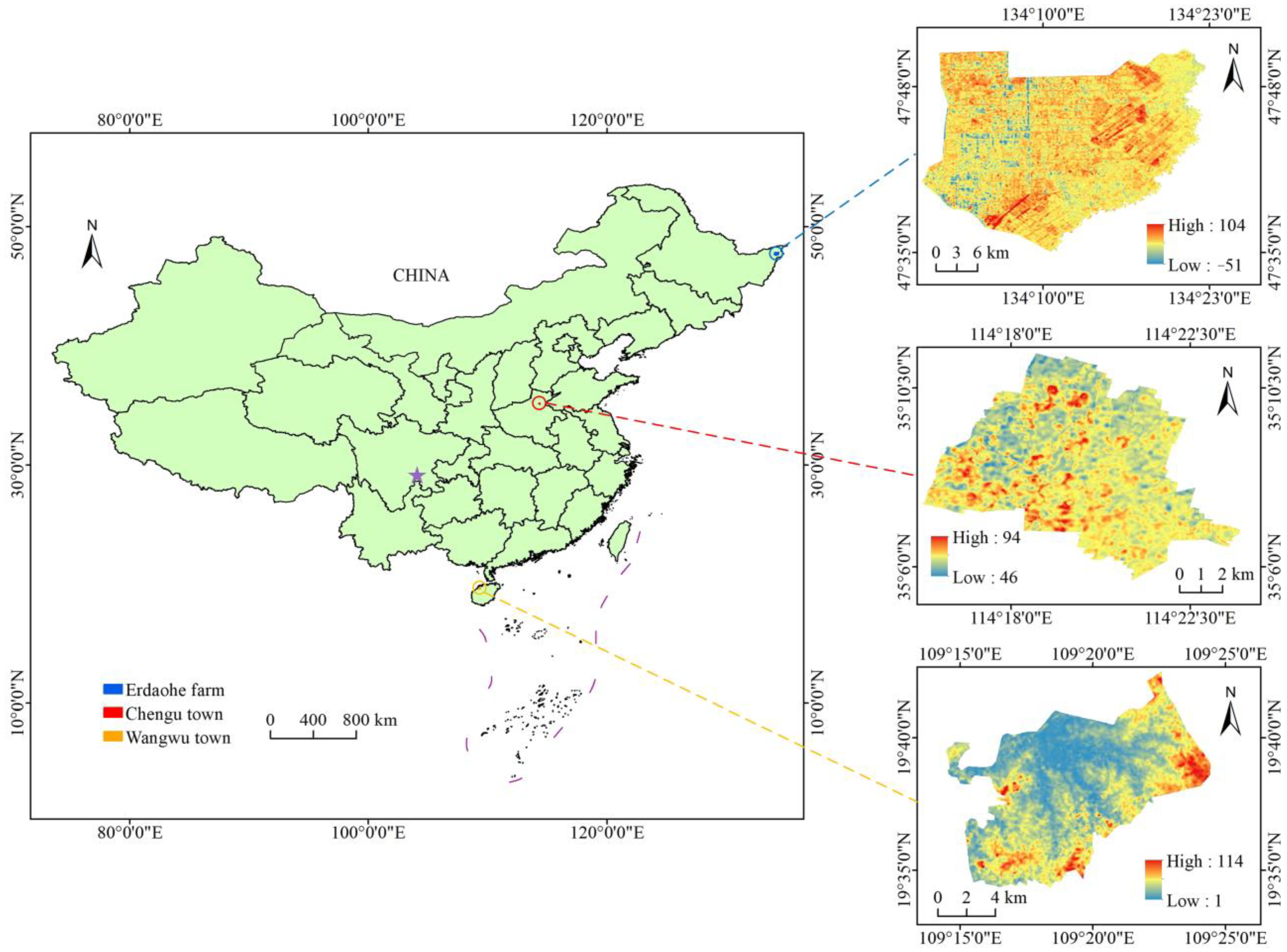
2.1. Study Area

In this paper, we selected three study areas located in different latitudes of China, each with high agricultural cropping intensity. The three study areas selected for the construction of the fusion dataset were located in Erdaohe Farm, Fuyuan City, Jiamusi City, Heilongjiang Province (SA1); Chengu Town, Fengqiu County, Xinxiang City, Henan Province (SA2); and Wangwu Town, Danzhou City, Hainan Province (SA3). In addition, a new study area was selected to test the spatial variability of the dataset, which was located in Longchi Town, Xuzhou District, Yibin City, Sichuan Province (SA4). The locations of the four study areas are shown in Figure 1. The images from the four study areas were projected in WGS 1984 UTM Zone 53 N (SA1), Zone 50 N (SA2), Zone 49 N (SA3), and Zone 48 N (SA4).
SA1 is subordinate to Sanjiang Plain, with geographical coordinates ranging between 47°35′3.50″N–47°55′55.45″N and 134°0′29.86″E–134°22′50.59″E. The area covers a total area of 54.30 thousand hectares, including 36.31 thousand hectares of cultivated land with rice, wheat, corn, and soybeans as crops, mainly rice. The planting system in this area is one crop per year. SA1 has a humid or semi-humid continental monsoon climate in the northern temperate zone, with low and flat terrain and fertile soil.
SA2 covers an area between 35°5′82.82″N–35°11′22.43″N and 114°15′45.62″E–114°23′44.77″E. The town has a total area of approximately 6.10 thousand hectares, including 23 administrative villages and about 4.53 thousand hectares of arable land. The topography of the area is flat, and the texture of the soil is mainly loamy and clayey, with loamy soils predominating. The study area has a semi-arid, semi-humid warm temperate continental monsoon climate characterized by a mean annual air temperature of around 14.5 °C and an annual precipitation of about 600 mm. The main crops grown in this area are winter wheat and summer maize, with a cropping system that matures twice a year.
SA3 is located in the northwest of Danzhou City, covering an area between 19°42′29.95″N–19°34′19.26″N and 109°14′27.50″E–109°24′27.47″E. SA3 has a total area of 14.35 thousand hectares, including one community and eight administrative villages. SA3 has a tropical monsoon climate, and the crop rotation pattern in the region mainly consists of two or three crops per year, with rice as the main crop.
SA4 covering an area between 28°54′4.27″N–29°0′43.87″N and 104°3′32.47″E–104°10′44.12″E. SA4 has a total area of 6.89 thousand hectares, including one community and seven administrative villages. The area is characterized by a subtropical humid climate, featuring copious rainfall and abundant sunshine.

2.2. Satellite Imagery and Its Characteristics

2.2.1. Landsat 8 OLI Satellite Imagery

Equipped with two sensors, the OLI and the Thermal Infrared Sensor (TIRS), the L8 satellite provides valuable data for a wide range of applications. The OLI sensor features nine bands with a spatial resolution of 30 m, except for the panchromatic band, which has a resolution of 15 m. The temporal resolution of the OLI sensor is 16 days, and the approximate scene size is 170 km north–south by 183 km east–west [28,29]. The image acquisition platform for the L8 OLI sensor is the Google Earth Engine (GEE, https://earthengine.google.com/ (accessed on 19 September 2022)), which offers L1TP (Terrain Precision Correction) and Land LaSRC (Surface Reflectance Code) products for the OLI sensor [30]. The L1TP product represents the image product after precision correction using ground control points (GCPs) and digital elevation model (DEM) data. On the other hand, the LaSRC product is the SR product after correction using the internal algorithm. In this study, we have selected the LaSRC products for our analysis.

2.2.2. Sentinel-2 MSI Satellite Imagery

The S-2 satellites, consisting of the two MSI remote sensing satellites, S-2A and S-2B, were successfully launched by the European Space Agency (ESA) on 23 June 2015 and 7 March 2017, respectively [31]. The S-2 MSI boasts a high temporal resolution with a revisit period of just 5 days. The MSI sensor includes 13 spectral bands with 10 m, 20 m, and 60 m spatial resolutions, respectively. In this study, images were acquired using the Google Earth Engine (GEE) platform, which provides two processing levels: Level-1C and Level-2A. The Level-1C products represent orthorectified, top-of-atmosphere reflectance, while the Level-2A product is the SR product with atmospheric correction based on Level-1C. The Level-2A product was selected for use in this study.

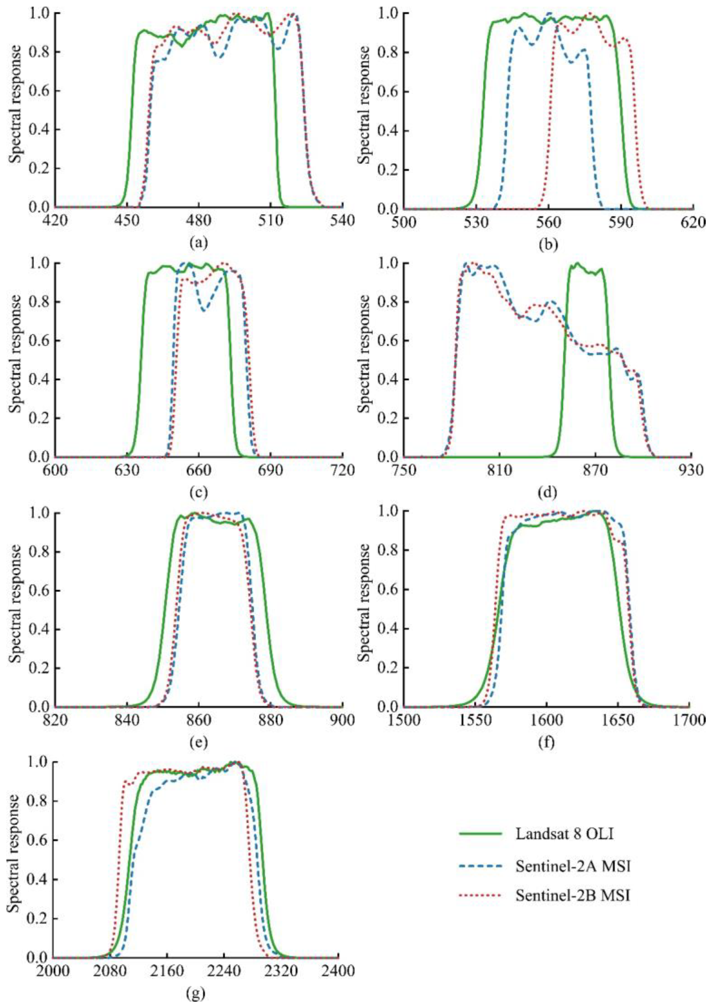
2.2.3. Comparison of Spectral Band Information and Spectral Response Functions

The L8 OLI and S-2A/B MSI sensors both contain coastal aerosol and cirrus bands. The coastal aerosol band is mainly used to monitor aerosols in the near-shore water and atmosphere, while the cirrus band is used to monitor water vapor content and cirrus cloud distribution in the atmosphere. These bands are not primarily used to monitor vegetation growth status. Therefore, this study only compared the other common bands (blue, green, red, near-infrared (NIR), shortwave infrared 1 (SWIR1), and shortwave infrared 2 (SWIR2) between these sensors. In addition, the S-2A/B MSI sensor includes a wide NIR band (NIR-8) and a narrow NIR band (NIR-8A), so the NIR band of the L8 OLI sensor was used to be compared with the NIR-8 and NIR-8A bands of the S-2A/B MSI sensors, respectively. The basic information of the common bands of the S-2A MSI, S-2B MSI, and L8 OLI sensor is shown in Table 1, and the spectral response function (SRF) curves are illustrated in Figure 2.
Table 1 shows that the spatial resolution of the blue, green, red, and NIR-8 bands of the S-2 MSI sensor is 10 m, and the spatial resolution of the NIR-8A, SWIR1, and SWIR2 bands is 20 m, while the spatial resolution of all bands of the L8 OLI sensor is 30 m. To ensure consistency in spatial resolution for corresponding bands, the nearest-neighbor interpolation method was used to resample the spatial resolution of the two sensors to 10 m first [32].
The central wavelength, bandwidth, and SRF curves of different sensors are slightly different (Table 1 and Figure 2). Except for the central wavelength and bandwidth of the SWIR2 band, which differ slightly (with a central wavelength difference of 16.7 nm and bandwidth difference of 10.0 nm), there is almost no difference between the corresponding bands of the S-2A MSI and S-2B MSI sensors. The SRF curves of the S-2A MSI and S-2B MSI sensors also almost overlap.
As shown in Figure 2, the variability of the SRF of L8 OLI and S-2A/B MSI in the NIR band is the largest, followed by the blue band, while the SWIR1 band is the closest. There are also subtle differences between the corresponding bands of L8 OLI and S-2A/B MSI (Table 1). More specifically, for the blue band, the central wavelength of the L8 OLI sensor differs from that of the S-2A MSI and S-2B MSI sensors by 10.4 nm and 10.1 nm, respectively. For the green band, the bandwidth of L8 OLI differs from S-2A MSI and S-2B MSI by 25 nm and 24 nm, respectively. As for the red band, the central wavelength and bandwidth of L8 OLI have slight differences compared to S-2A/B MSI.
The above analysis shows that the differences between the bands of the S-2A/B MSI and L8 OLI sensors are generally subtle, which makes the collaborative application of these sensors possible. However, due to the existence of these subtle differences, the images of these sensors should not be directly substituted in the process of collaborative application. Necessary spectral information adjustments must be made.

2.3. Selection of Image Pairs

To minimize biases arising from temporal and surface condition disparities, we made the deliberate choice to examine L8 OLI and S-2A/B satellite images acquired synchronously on a single day. For the experiment, we carefully selected seven pairs of high-quality images, two image pairs each for SA1, SA2, and SA3, and one image pair for SA4. Each image pair was chosen based on favorable insolation and atmospheric conditions, and closely matching solar zenith and azimuth angles. This meticulous selection process ensured the consistency of observed characteristics between the two sensors. Detailed information regarding these image pairs can be found in Table 2.
Figure 3 illustrates the seven image pairs in their original spatial resolution. As depicted in Figure 3, these image pairs exhibit minimal cloud cover. Moreover, the 10 m resolution provides enhanced spatial detail for the same geographical area, enabling improved delineation of farmland boundaries and offering more comprehensive information on farmland characteristics. To assess the correlation between corresponding bands in image pairs at 10 and 30 m spatial resolutions, the nearest-neighbor interpolation method was employed to resample the seven image pairs. The resulting resampled images yielded 7,981,833 and 889,237 single-band pixels for SA1, 788,488 and 88,243 for SA2, and 1,391,474 and 155,582 for SA3 at the respective spatial resolutions of 10 and 30 m, respectively.

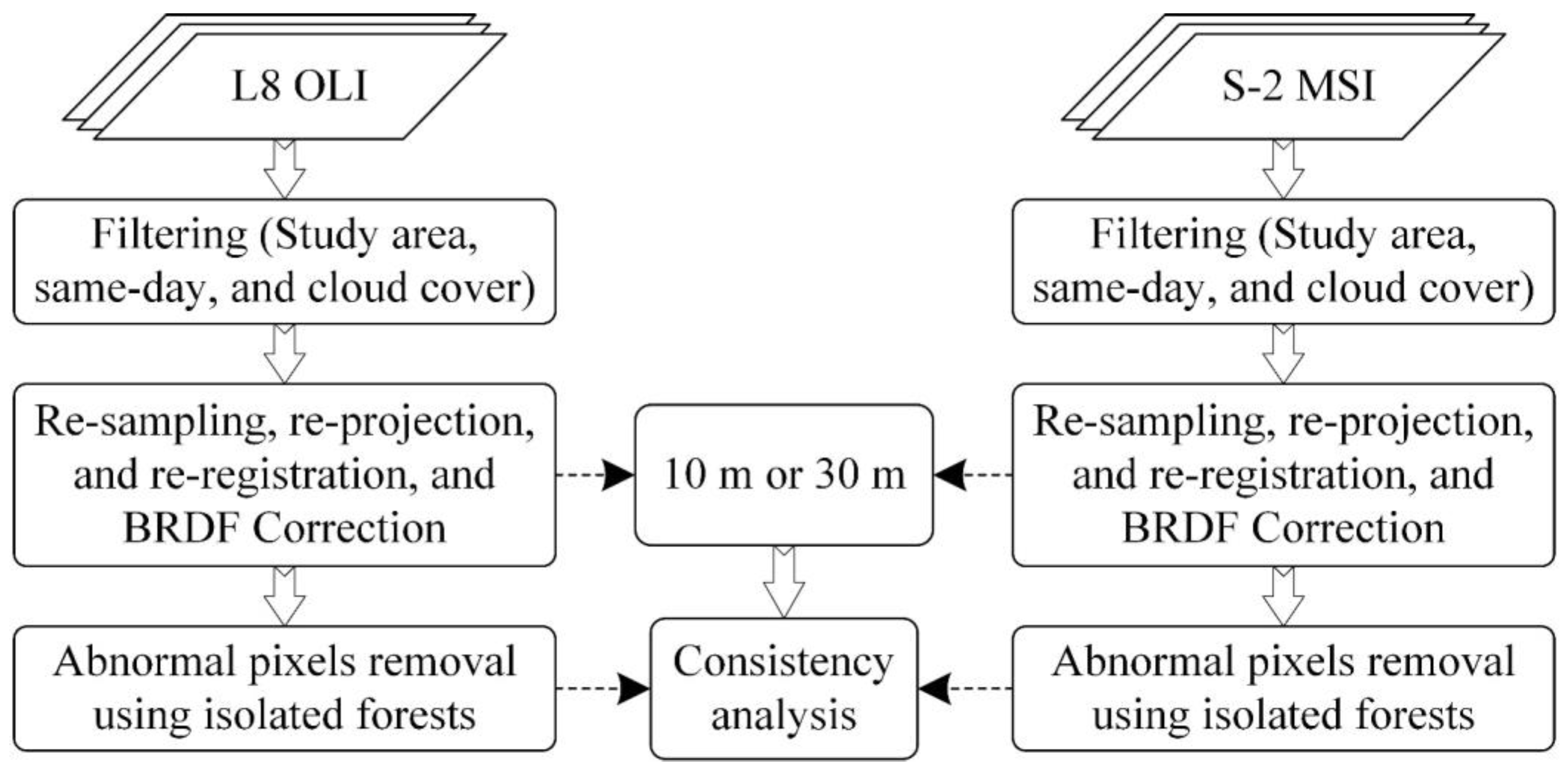
2.4. Flow of Harmonized Consistency Analysis

In this study, we introduced the iForest algorithm to eliminate outlier anomalous pixels in the study area and prevent the anomalies from affecting the accuracy of subsequent band consistency exploration between two satellite sensors (Figure 4). We utilized the GEE platform to obtain six same-day image pairs, each containing both L8 and S-2 images, from three study areas with high crop planting density. The acquired image pairs were then preprocessed with cloud masking, re-projection, and re-registration, with a nearest-neighbor interpolation method used for resampling to 30 m and 10 m, respectively. To reduce reflectance differences caused by differences in imaging geometry, we employed the C-factor bidirectional reflectance distribution function (BRDF) correction method. Then, we extracted spectral reflectance values from the corresponding spectral bands and spatial locations of L8 OLI and S-2 MSI images, and anomalous pixels were removed from the image pairs using the iForest algorithm. Finally, the correlation of the image pairs was analyzed.

2.5. C-Factor BRDF Correction

The c-factor BRDF correction approach is a commonly used technique for correcting the effects of illumination and viewing geometry on the BRDF of a surface [33]. The BRDF describes the amount of light reflected by a surface in different directions for a given illumination and viewing geometry. However, the BRDF can vary significantly depending on the illumination and viewing geometry, making it challenging to compare BRDF measurements made under different conditions.
The c-factor BRDF correction approach involves measuring the reflectance of a surface under various illumination and viewing geometries, and using these measurements to calculate a normalization factor, the c-factor. The c-factor accounts for variations in the BRDF caused by changes in illumination and viewing geometry and can be used to normalize BRDF measurements made under different conditions. This approach enables more accurate comparisons between BRDF measurements and facilitates the creation of more consistent and reliable BRDF models.

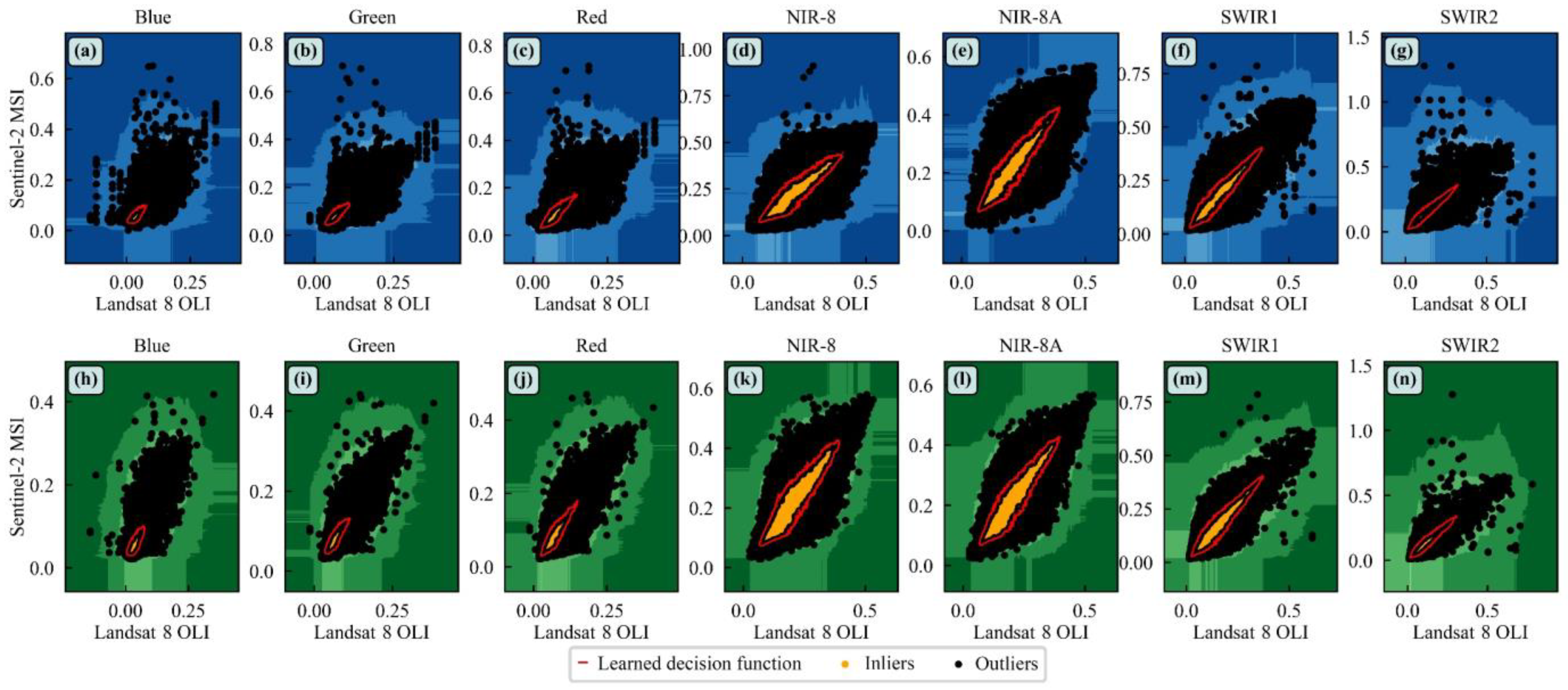
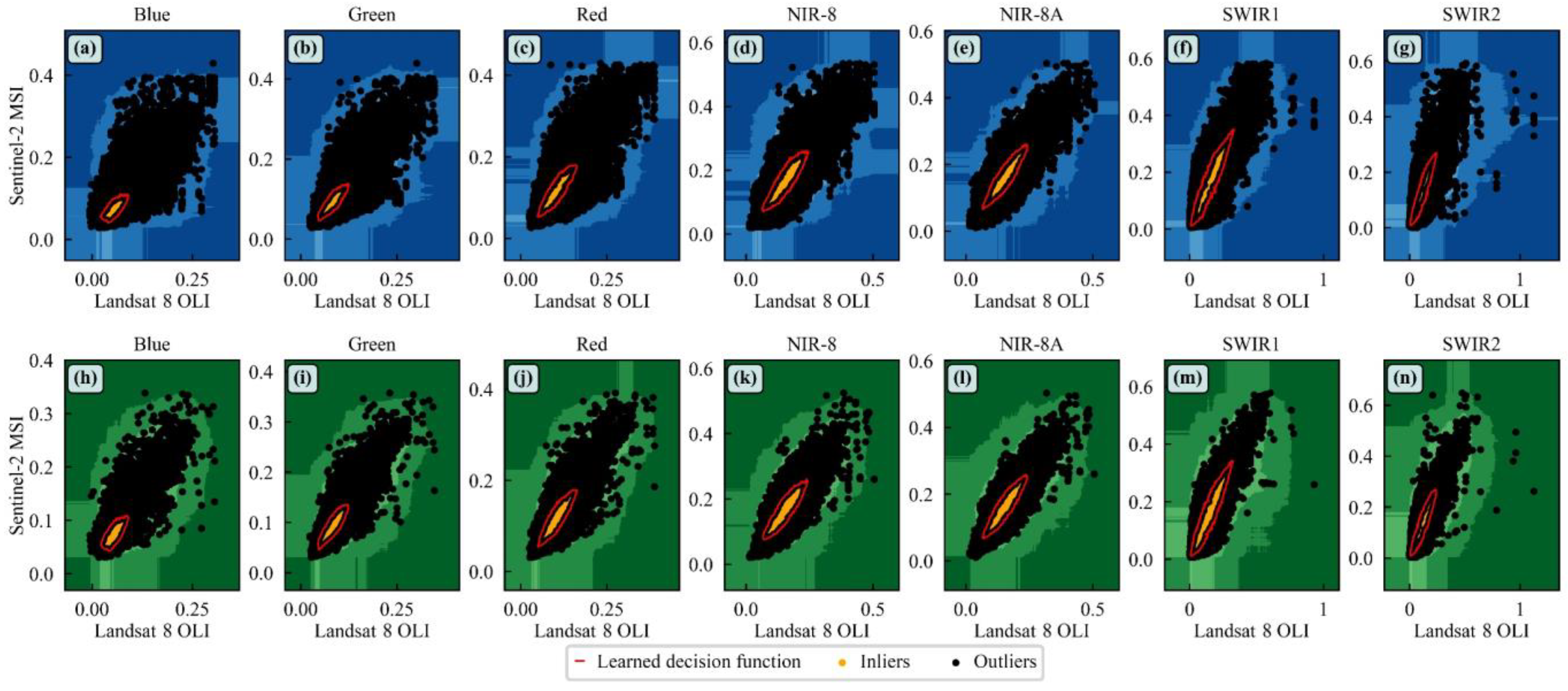
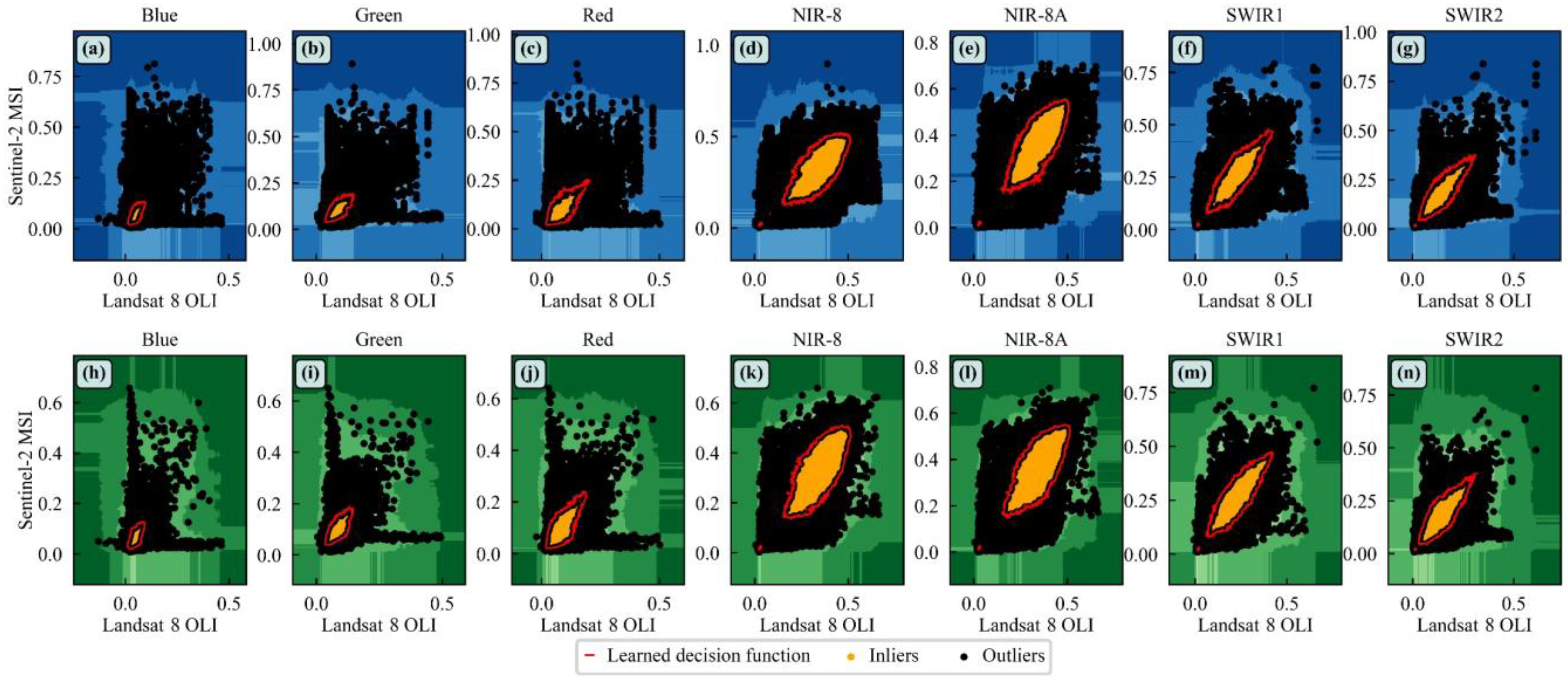
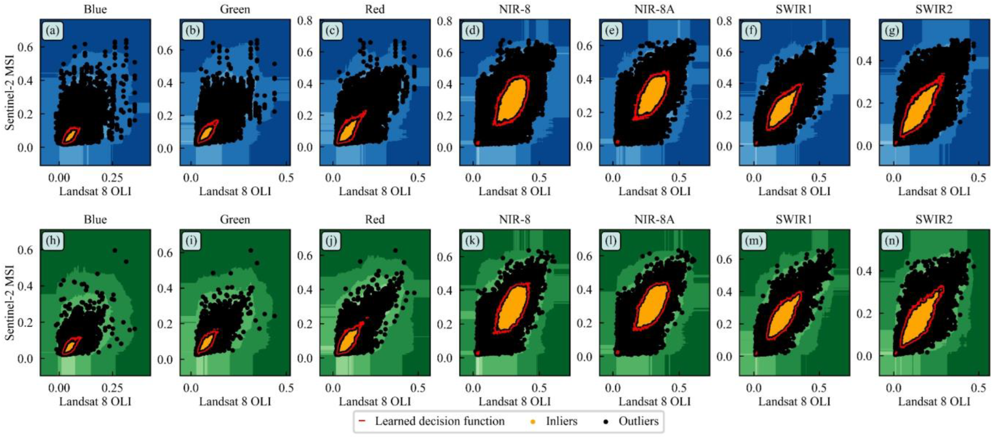
2.6. Isolation Forest Algorithm

The isolation forest (iForest) algorithm is an unsupervised anomaly detection method based on integrated learning, which has the advantages of high detection accuracy, low time complexity, and low consumption of computing resources [34]. This approach defines the sparsely distributed data, which is far away from the high-density data population, as the anomalous isolated sparse points. The iForest algorithm operates by randomly selecting a feature and a value within the range of that feature to create a splitting rule. This rule is used to recursively partition the data until each data point is isolated in its own partition. High-density data require multiple cuts to be separated, while outlier data will be isolated earlier. Unlike other quantitative indicators that rely on distance and density to portray the degree of sparsity between data, the iForest algorithm isolates sample points without calculating distance and density, leading to a faster algorithm and higher detection accuracy [35,36].
According to the characteristics of the ensemble algorithm, the individual isolated trees are independent of each other and can be used on datasets with massive data [37]. The use of iForest anomaly detection techniques to remove outlier samples from image datasets can provide a useful idea to further improve the correlation of image pairs.

2.7. Statistical Analysis

In this study, we employed an ordinary least squares regression to obtain linear adjustment coefficients of L8 OLI and S-2A/B MSI sensor images. OLS regression model is a common technique for estimating coefficients of linear regression equations, which describe the relationship between one or more independent variables and a dependent variable [38]. The model estimates the relationship by minimizing the sum of the squares in the difference between the observed and predicted values of the dependent variable configured as a straight line. In this study, OLS regression will be discussed in the context of a bivariate model, which is based on only one independent variable (x) and one dependent variable (y). The significance and accuracy of the OLS regression model were evaluated by qualitative and quantitative analysis methods.

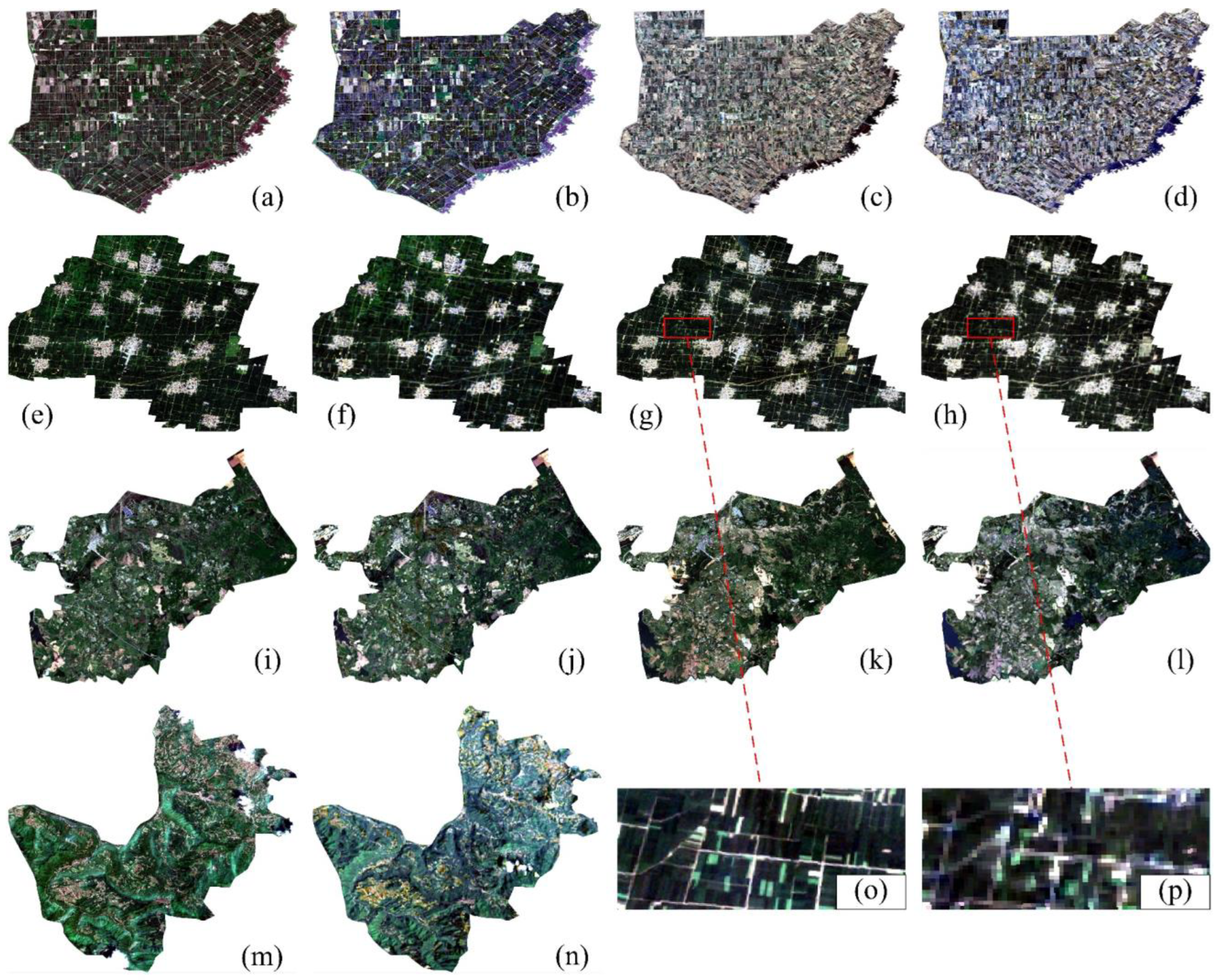
2.7.1. Qualitative Analysis

The significance test of the OLS regression model usually uses the F-test to test the significance of the regression effect and to qualitatively analyze the quality of fit of the regression equation. The sum of squares total (SST) can be decomposed into the sum of squares regression (SSR) and the sum of squares error (SSE).
i = 1 n y i y ¯ i 2 = i = 1 n y ^ i y ¯ i 2 + i = 1 n y i y ^ i 2
where i = 1 n y i y ^ i 2 is the SST, which measures the degree of variation of the dependent variable y; i = 1 n y ^ i y ¯ i 2 is the SSR, which measures the degree of variation between the actual and fitted values; and i = 1 n y i y ¯ i 2 is the SSE, which measures the degree of variation of the fitted values of the dependent variable y. The degrees of freedom fT, fA, and fE for SST, SSA, and SSE are n − 1, 1, and n − 2, respectively.
The F-test is presented below, starting with the statistical hypothesis: b = 0 and the statistic F defined as
F = SSR / f A SSE / f E = SSR SSE / n 2 ~ F 1 , n 2
The significance level α is known, and the critical value F 1 , n 2 can be found by checking the F distribution table, and the regression equation is regarded as significant if F > F α .

2.7.2. Quantitative Analysis

In this study, root mean square error (RMSE) and mean absolute error (MAE) were used as metrics to quantitatively evaluate the accuracy of the estimation models. The RMSE reflects the degree of dispersion between the predicted and measured values, and the MAE describes the average model performance error. The specific formulas for calculating RMSE and MAE are as follows:
RMSE = 1 N i = 1 N y i y ^ i 2
MAE = 1 N i = 1 N y i y ^ i
where N is the number of samples, y i indicates the observed values for sample i, and y ^ i is the predicted values.

3. Results

3.1. Quantitative Spectral Conversion Relationships for Different Latitudinal Farming Regions

The outlier samples in the image pairs are removed using the iForest anomaly detection technique, and the removal results for SA1 are shown in Figure 5 and Figure 6, and those of SA2 and SA3 are shown in Figure A1, Figure A2, Figure A3 and Figure A4. The iForest anomaly sample ratio is set to 0.05 based on research experience and multiple experimental validations [39]. After removing the anomalous pixels, the pixels in SA1 single-band images were 7,582,746 and 844,775, 749,063 and 83,830 in SA2, and 1,321,900 and 147,802 in SA3 when the spatial resolution was 10 m and 30 m, respectively. As can be seen in Figure 5 and Figure 6, the outlier pixels were mostly discrete data. Therefore, we found that the iForest algorithm could effectively screen out outlier pixels and isolate anomalous pixels (black dots), then remove the anomalous information in the satellite images.
After removing the anomalous pixels using the iForest algorithm, the spectral reflectance of the L8 OLI satellite sensor is used as the independent variable, and the spectral reflectance of the S-2 MSI sensor is used as the dependent variable. Using the OLS regression model in the Python environment, the corresponding spectral bands of these two satellite sensors (including blue, green, red, NIR-8, NIR-8A, SWIR1, and SWIR2 bands) are fitted with a one-dimensional linear fit. For SA1T1, the fitting results for spatial resolutions of 10 m and 30 m are shown in Figure 7 and Figure 8, respectively. For SA1T2, the fitting results with a spatial resolution of 10 m and 30 m are shown in Figure 9 and Figure 10, respectively. For SA2 and SA3, the relationships between the corresponding spectral bands of L8 OLI and S-2 MSI are shown in Figure 11 and Figure A5, Figure A6, Figure A7, Figure A8, Figure A9, Figure A10, Figure A11 and Figure A12.
As can be seen from Figure 7 and Figure 9, for SA1, when the spatial resolution of the corresponding bands of the L8 OLI and S-2 MSI sensors is resampled to 10 m, the Pearson correlation coefficients between the six corresponding bands, except for the blue band, all exceed 0.88. In particular, for the SWIR1 and SWIR2 bands, the correlation coefficients of SA1T1 were both 0.98 and the correlation coefficients of SA1T2 were also both 0.98. At a spatial resolution resampling of 30 m (see Figure 8 and Figure 10), the Pearson correlation coefficients between the corresponding bands of both satellite sensors almost exceed 0.90 (except for the blue band). The reason for the low correlation between the Blue band of the two sensors is that the blue band of the L8 OLI sensor SR product has been used in the algorithm to perform aerosol inversion tests and is therefore unreliable [40].
For SA2, when the spatial resolution of both sensors is resampled to 10 m (see Figure 11 and Figure A5, Figure A6, Figure A7 and Figure A8), the Pearson correlation coefficients between the corresponding bands exceed 0.89 (the average correlation coefficients of SA2T1 and SA2T2 are 0.93 and 0.94, respectively). At a spatial resolution of 30 m, the Pearson correlation coefficients between the corresponding bands of both satellite sensors exceeded 0.93 (the average correlation coefficients of SA2T1 and SA2T2 are 0.94 and 0.95, respectively). For SA3, the average Pearson correlation coefficients between the corresponding bands of SA3T1 and SA3T2 were 0.83 and 0.84, respectively, when the spatial resolution of the two sensors was resampled to 10 m (see Figure 11 and Figure A9, Figure A10, Figure A11 and Figure A12). The average Pearson correlation coefficients between the corresponding bands of SA3T1 and SA3T2 at a spatial resolution of 30 m were 0.84 and 0.85, respectively. In addition, from Figure 7, Figure 8, Figure 9 and Figure 10, it can be found that the NIR band of L8 OLI is more correlated with the NIR-8A band of S-2 MSI than the NIR-8 band, which is due to the fact that the central wavelength and bandwidth of the NIR-8A band of S-2 are more similar and closer to the NIR band of L8 OLI.
As shown in Figure 3o,p, the 10 m spatial resolution image enhances the delineation of edges and details of diverse farmland landscape types, facilitating more accurate detection and monitoring of crop growth dynamics and changes over time. As can be seen from Figure 11, by comparing the average Pearson correlation coefficients of all bands in the six image pairs, it can be found that the band’s correlation relationship of images with a spatial resolution of 30 m is slightly higher than that of 10 m. The mean Pearson correlation coefficients of the six image pairs with spatial resolutions of 10 m and 30 m were 0.89 and 0.90, respectively. The results show that when the spatial resolution of both L8 OLI and S-2 MSI corresponding bands are resampled to 10 m using the nearest-neighbor interpolation method, the corresponding bands of these two sensors can be quantitatively converted and applied synergistically.
Based on the comparison of the three study landscapes (Figure 11), it was observed that the Pearson correlation coefficients of all the corresponding bands were lowest in SA3, at spatial resolution resampling of 10 m and 30 m, as compared to the other two study areas. The low correlation between L8 OLI and S-2 MSI in SA3 could be attributed to the tropical monsoon climate of the southern region of China, where this landscape is situated (low latitude), resulting in higher susceptibility to the influence of clouds, rain, and other weather conditions during remote sensing processes. Despite selecting images with minimal relative cloud interference, the low latitude region still experienced higher levels of cloud interference compared to the other two regions.

3.2. Adjustment Coefficients Derived for Integrated L8 and S-2 Data with High-Spatial Resolution at Mixed Latitudes

By examining the correlation between the corresponding bands of L8 and S-2 images, it can be observed that the Pearson correlation coefficients of these two sensors were consistently high in the high, middle, and low latitudes of China (refer to Figure 11). Moreover, the correlation between the corresponding bands of these two sensors at a spatial resolution resampling of 10 m differs little from the 30 m spatial resolution. Consequently, considering the practical requirements for farmland monitoring in China, we tried to integrate the data with a 10 m spatial resolution at various latitudes in order to derive adjustment coefficients derived from integrated L8 and S-2 data.
First, the anomalous pixels of these six pre-processed image pairs with 10 m spatial resolution were removed using the iForest algorithm and recorded. Then, we randomly selected 100,000 pixels in each image pair after the anomaly detection process and combined them into a multi-latitude dataset as the training set (randomly selecting the same pixels in each image pair can effectively reduce the impacts caused by the different numbers of pixels). After that, the spectral reflectance of the L8 OLI sensor was used as the independent variable, the spectral reflectance of the S-2 MSI sensor was adopted as the dependent variable, and the OLS regression algorithm was employed to perform a one-dimensional linear fit.
Finally, the adjustment coefficients derived from integrated L8 and S-2 data with high-spatial resolution at mixed latitudes were obtained. The scatterplots of the linear fitting results of the two sensors with 10 m spatial resolution are shown in Figure 12, and the adjustment coefficients of the two sensors at mixed latitude are presented in Table 3.
As it can be seen from Figure 12 and Table 3, when the spatial resolution of the corresponding bands of the two sensors were resampled to 10 m, the Pearson correlation coefficients between the other six corresponding bands exceeded 0.84, except for the blue band (the Pearson correlation coefficient for the blue band was 0.72). Therefore, we can find that there was also excellent consistency among the mixed latitude datasets. It proves that it is feasible to construct the adjustment coefficients derived for integrated L8 and S-2 data with a high-spatial resolution by mixing the datasets of the high, mid, and low latitude regions of China.
Then, we tested the significance of the conversion equations for the seven corresponding bands of the two sensors by F-test. We calculated the values of the statistics F for the seven models by scipy.stats.levene in a Python environment and obtained the F values of 55.82, 16,630.82, 9587.21, 1170.60, 734.40, 3383.00, and 5886.81 for the seven bands, respectively. It can be seen that when the significance level α was 0.01, the F values of the seven bands were greater or much greater than the critical value F 0.01 . The probability of overlap between the regression equation and the actual equation is 99%, and the seven regression equations are highly significant. Therefore, the overall significance test of the seven regression models passed.
Subsequently, we conducted a quantitative analysis of the seven regression equations. To this end, we randomly selected 10,000 pixels in each corresponding band of two image pairs at high, middle, and low latitudes, respectively, as test sets. These test sets were then input into the regression equations to calculate the values of RMSE and MAE. The calculation results are presented in Table 4. As can be seen from Table 4, the RMSE and MAE of the regression equations for the six bands are within 20% of the mean value of the training set, except for the blue band (the mean reflectance values for the seven bands of the S-2 sensor are 0.041, 0.065, 0.058, 0.269, 0.271, 0.165, and 0.097, respectively). This indicates that the established regression equation has a high accuracy and an excellent conversion effect.
The results above demonstrate the significant and accurate performance of the adjustment coefficients derived from integrated L8 and S-2 data, both qualitatively and quantitatively.
Furthermore, we examined the spatial heterogeneity of these adjustment coefficients. We input the original L8 OLI sensor imagery from SA4 into the regression equation to correct the L8 OLI data. Subsequently, we calculated the values of RMSE and MAE for each band using the corrected L8 OLI data and the original S-2 MSI data. The test results indicated that all bands exhibited favorable performance (Table 5). These findings support the robustness and spatial heterogeneity of the adjustment coefficients.
In the following section, we apply the adjustment coefficients to various crop-growing areas in China, exploring the advantages of these adjustment coefficients in monitoring crop growth status.

3.3. Application Examples of Adjustment Coefficients Derived for Integrated L8 and S-2 Data with High-Spatial Resolution at Mixed Latitudes

To verify the advantages of the adjustment coefficients derived for integrated L8 and S-2 images in monitoring crops, this study selected one representative pixel site in each study area to monitor the normalized difference vegetation index (NDVI) time series variation in different latitudes. First, all L8 and S-2 images covering each pixel site in the delimited time range were acquired separately and pre-processed with cloud masking, re-sampling, re-projection, re-registration, and BRDF correction. Then, the obtained adjustment coefficients were input into the L8 images and merged with the S-2 images. Finally, the NDVI values of the integrated images were calculated to construct the NDVI time series, and the NDVI time series were smoothed with the Savitzky-Golay smoother. The results of the NDVI time series curves plotted for the three-pixel sites are shown in Figure 13. As the image pairs selected for calculating the adjustment coefficients of these adjustment coefficients were for the years 2020 and 2021 (see Table 1), the time range selected for this example is the full year period of 2019 in order to highlight the temporal extrapolation and scalability of this adjustment coefficients. For a single satellite sensor, it is possible for a pixel site to be covered by multiple images on the same day due to the distribution of image stripes. Therefore, we averaged the NDVI values of all images taken on the same day. In addition, it can be seen from Figure 11 that the correlation between the NIR-8A band was higher than that of the NIR-8 band, so we used the NIR-8A band to calculate the NDVI values, which in turn can more accurately reflect the changes in the growth status of crops.
The selected pixel site at a high-latitude region (SA1) mainly cultivated with rice crops. The planting system is one crop per year. Rice in this pixel site is planted in late April and harvested in early October. In the mid-latitude region (SA2), the selected pixel site is a winter wheat–summer corn rotation pattern. Winter wheat is planted in early October and harvested in late May the following year; summer corn is planted in early June and harvested in late September. The selected pixel site in the low-latitude region (SA3) is a three-season cropping system per year containing a double-season rice crop (early and late rice) and a one-season wax gourd crop. Early rice is planted in early March and harvested at the end of June; late rice is planted in early July and harvested in late November; and the wax gourd is planted in early December and harvested in early March of the following year.
As illustrated in Figure 13, the NDVI time series curves created using the integrated L8 and S-2 images accurately captured the variation in crop growth intensity within the high, middle, and low latitudes in China. Using only the S-2 images resulted in the appearance of outliers (e.g., 16 July 2019 of S-2 in Figure 13a, 3 April 2019 of S-2 in Figure 13c). Merging S-2 and L8 could correct the smoothed NDVI time series curves to more accurately describe crop growth and development changes. The study area SA3 (Figure 13c) is a typical cloudy area, and the observed images for constructing the NDVI time series were not as dense as the high-latitude region. However, most of the phenological stages of this three-season crop-growing system are clearly recognizable. Meanwhile, the NDVI time series curves can reflect the well-adjusted effect of adjustment coefficients. The NDVI values of the adjusted L8 and S-2 on the same day were closer than the original L8 and S-2 (e.g., 24 June 2019 in Figure 13b, 7 July 2019 in Figure 13b). In summary, we can find that the use of dense time series (integrated L8 and S-2 images) is sufficient to detect sharp changes in surface crop growth information, such as vegetation greening or crop harvest.
As shown in Figure 13, the total number of observed images was 77, 50, and 41 in the three-pixel sites, and the number of L8 observed images was 16, 19, and 11, respectively. It is noteworthy that the number of L8 images occupied a higher percentage, 21%, 38%, and 27%, respectively. The results indicated that both S-2 and L8 images performed an important filling role in the construction of NDVI time series curves.

4. Discussion

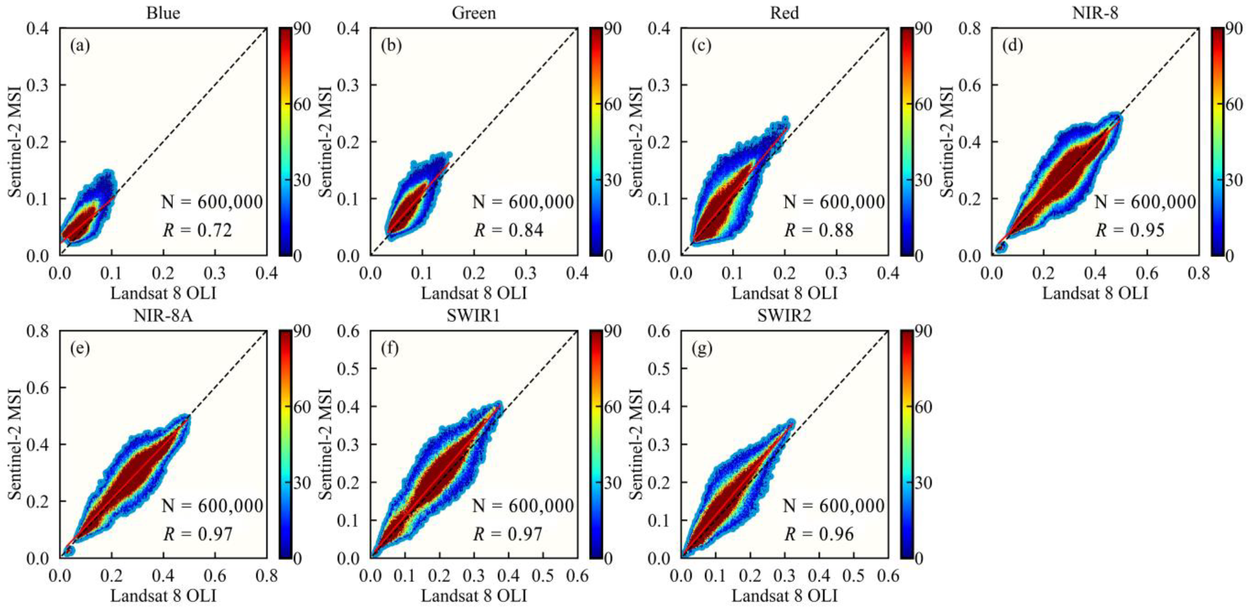
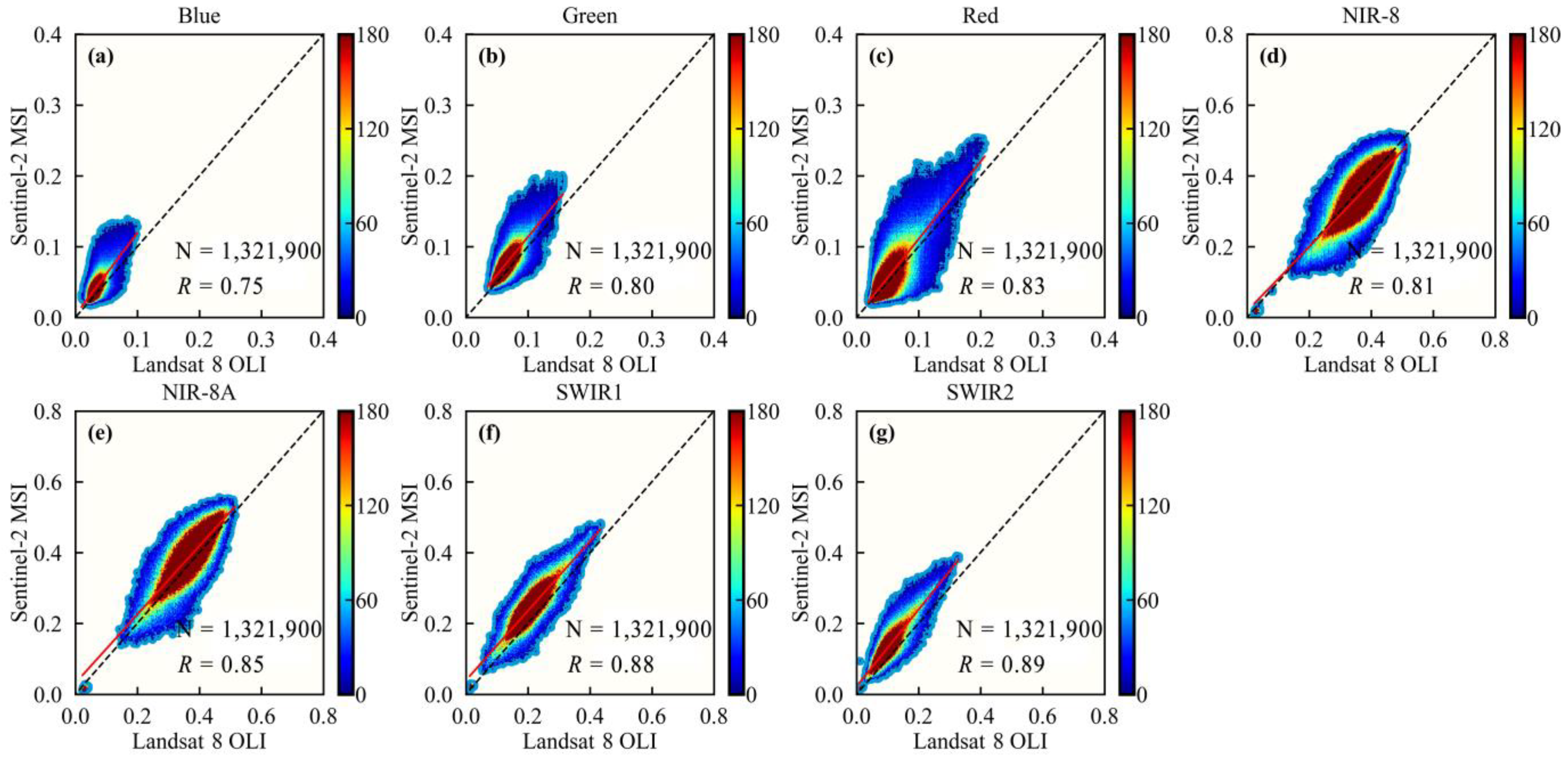
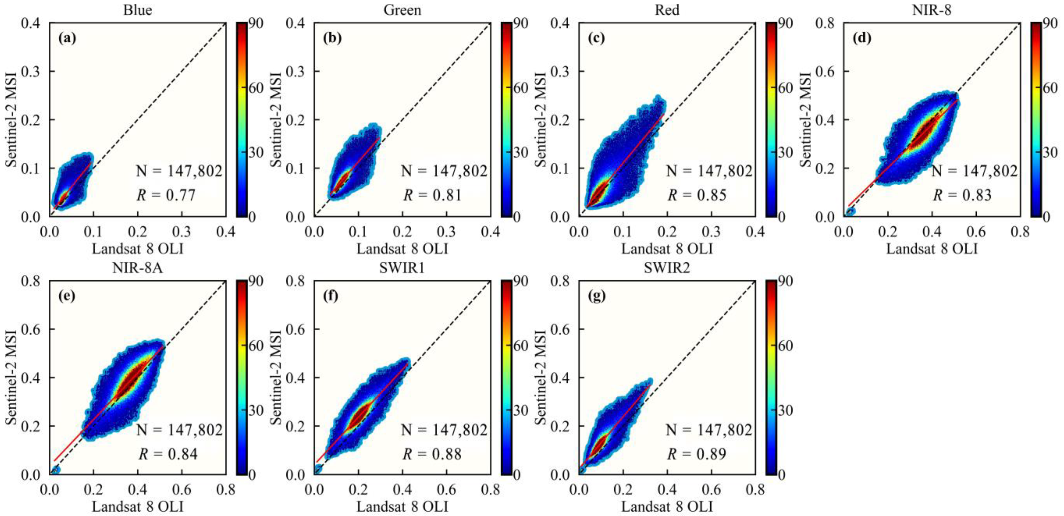
4.1. Comparison with Results without Outlier Processing

To verify the effectiveness of using the iForest algorithm in removing anomalous pixels from remote sensing images, the Pearson correlation coefficients of the corresponding bands of L8 OLI and S-2 MSI using and not using the iForest algorithm were compared for six synchronization periods (Figure 14). It is found that the use of the anomaly detection algorithm can effectively improve the correlation between the corresponding bands of the two sensors. At a spatial resolution of 10 m, the average Pearson correlation coefficients of SA1T1, SA1T2, SA2T1, SA2T2, SA3T1, and SA3T2 were improved by 0.007, 0.014, 0.029, 0.021, 0.075, and 0.021, respectively. It can be concluded that using the iForest algorithm can effectively improve the correlation between the corresponding spectral bands of L8 OLI and S-2 MSI sensors and reduce the variability between farming areas at different latitudes.
The iForest algorithm can remove the influence of anomalous pixels and improve the similarity of the image pairs to the corresponding bands. The iForest algorithm does not need to calculate the distance between data points, and the time complexity of the algorithm is linear. Meanwhile, the method uses an integrated learning strategy and has good detection performance for large datasets. Therefore, compared with the more complex algorithms for outlier removal in model theory, such as Density-Based Spatial Clustering of Applications with Noise (DBSCAN) [41] and Local Outlier Factor (LOF) [42], the iForest algorithm can effectively solve the problem of anomaly detection for large datasets in this study.
Moreover, the iForest algorithm has the advantages of faster operation speed and lower operation cost, but the iForest algorithm cannot establish the proportion of outliers adaptively, and further improvement of the method is needed for better application. Furthermore, there is a certain false detection rate using the iForest algorithm, and how to reduce the false detection rate needs further study.

4.2. Strengths and Weaknesses of Adjustment Coefficients Derived for Integrated L8 and S-2 Data with High-Spatial Resolution at Mixed Latitudes

Harmonizing satellite images from L8 OLI and S-2 MSI sensors is an effective way to obtain high spatial and temporal resolution data for earth observation and remote sensing modeling. In this study, we compared and evaluated the differences between L8 OLI and S-2 MSI sensors in different latitudes of farming areas in China and determined the quantitative conversion relationship between the corresponding spectral bands of the two sensors to obtain the robust adjustment coefficients derived for integrated L8 and S-2 data with high-spatial resolution at mixed latitudes. This ensured the spectral consistency of both sensors and realized the multi-source synergistic and complementary application of multi-spectral remote sensing data in farmland information monitoring. The National Aeronautics and Space Administration (NASA) has released a product that harmonizes L8 OLI and S-2 MSI (Harmonized Landsat Sentinel-2, HLS) and gives quantitative conversion equation coefficients [43]. This product matches the corresponding L8 OLI band by adjusting the surface reflectance of each S-2 MSI band, and the results of this study compared to the HLS product are shown in Table 6. However, this product is generated from identical simulated data, ignoring the possibility of differences due to variations in the ground environment or differences in observation conditions. In addition, it generates a spatial resolution of 30 m, which is a coarse resolution and not suitable for fine monitoring of crop growth status in small fields in China. In this study, the iForest algorithm is utilized to remove anomalous pixels with a spatial resolution of 10 m. This ensures that the images are spectral values of the real environment on the ground and excludes the influence of anomalous pixels. It also enables high-precision monitoring of regional farmland information in China.
This study will be of great enhancement to the subsequent studies on acreage extraction, crop growth status detection, and crop yield estimation of crops in agricultural cropping areas. However, due to the unsatisfactory effect of cloud removal, the NDVI time series curves of this study will show anomalous pixels (e.g., 29 March 2019 for S-2 and 2 April 2019 for L8 in Figure 13b), resulting in some deviations between the curves and the crop growth dynamics curves in the region. Meanwhile, the quality of the observed images at low latitudes is degraded by weather conditions, such as clouds and rain. To solve this problem, the fusion of optical images and synthetic aperture radar (SAR) images can be considered in the future to improve the observation accuracy and frequency of crop growth and development status.
In addition, the Pearson correlation coefficient in the blue band in this study is low (Figure 11 and Figure 12), and we can try to optimize it in the future using nonlinear regression models or deep learning methods, such as generative adversarial networks. Moreover, studies on the analysis and conversion of crop surface reflectance differences in subtypes of crop areas are still lacking, and further tests and in-depth discussions are needed.

5. Conclusions

The monitoring of crop growth and development greatly benefits from intensive time series observations. However, the limitations of single satellite systems, such as revisit cycles and weather conditions, hinder their ability to provide high-frequency and long-term observations required for crop growth monitoring in Chinese farmlands. To overcome these limitations, this study focuses on identifying quantitative conversion relationships between Landsat 8 OLI and Sentinel-2 MSI sensors and generating a high spatial-temporal resolution dataset using the isolated forest algorithm and linear regression analysis techniques. The dataset presented in this study provides continuous and detailed observational information, enabling a better understanding of crop growth dynamics, optimization of agricultural management, and crop yield prediction. This dataset performs a pivotal role in realizing precision agriculture, enhancing agricultural productivity, and promoting sustainable development in the agricultural sector. The main conclusions of the study are as follows:
(1)
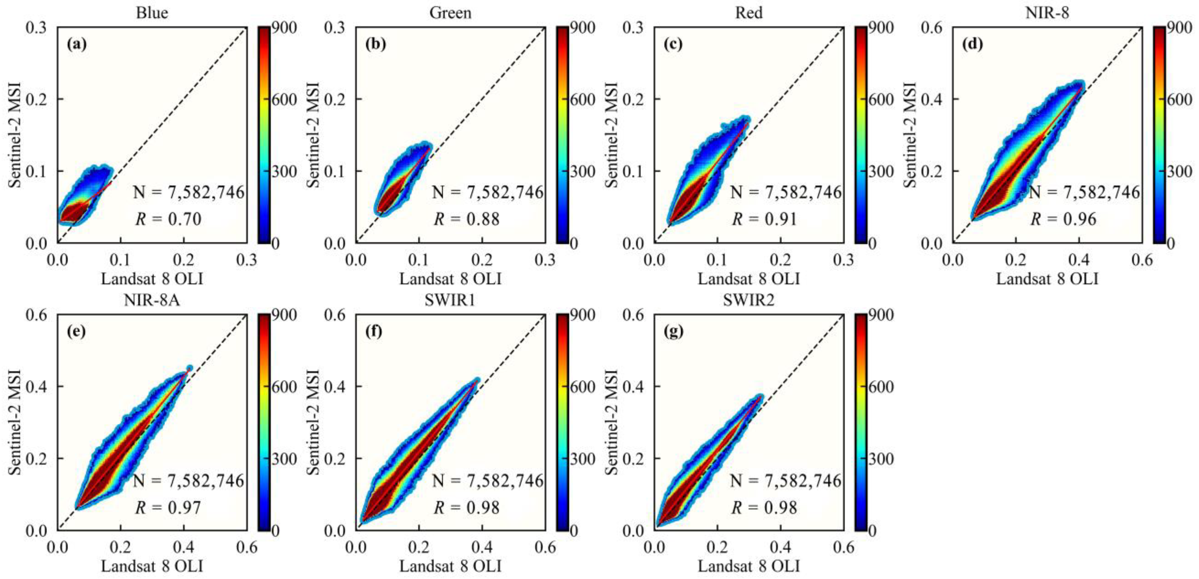
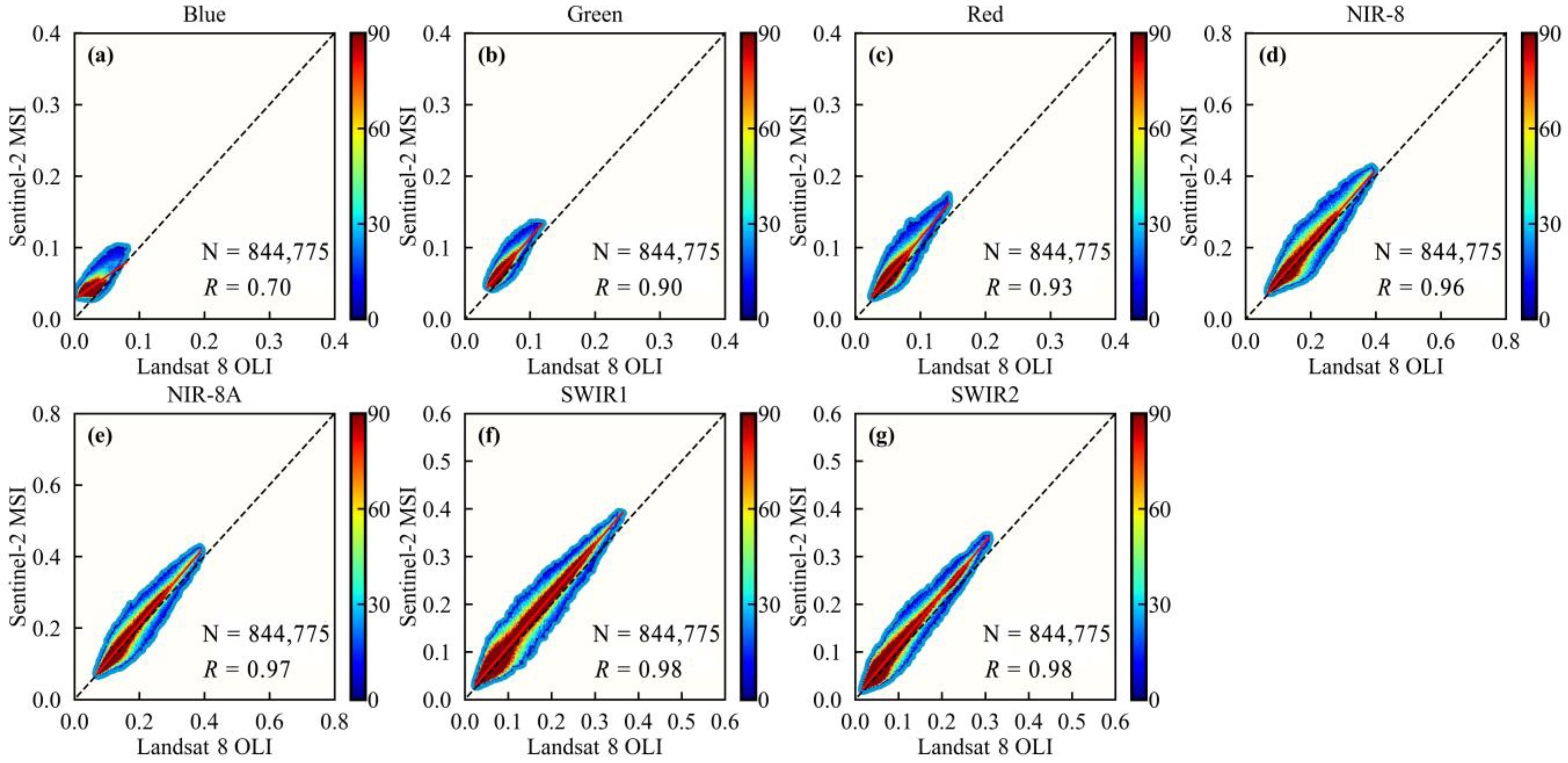
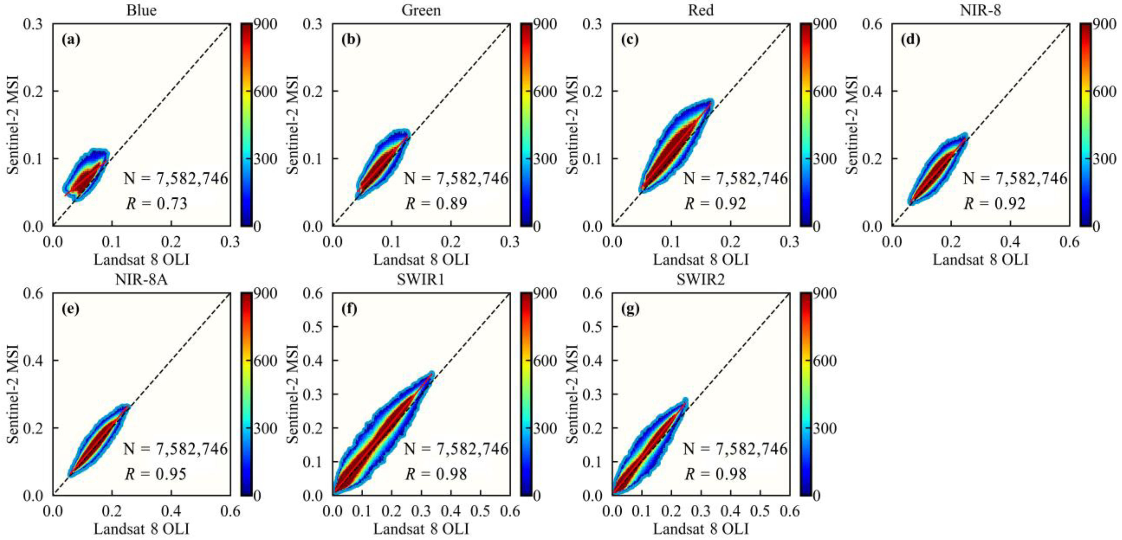
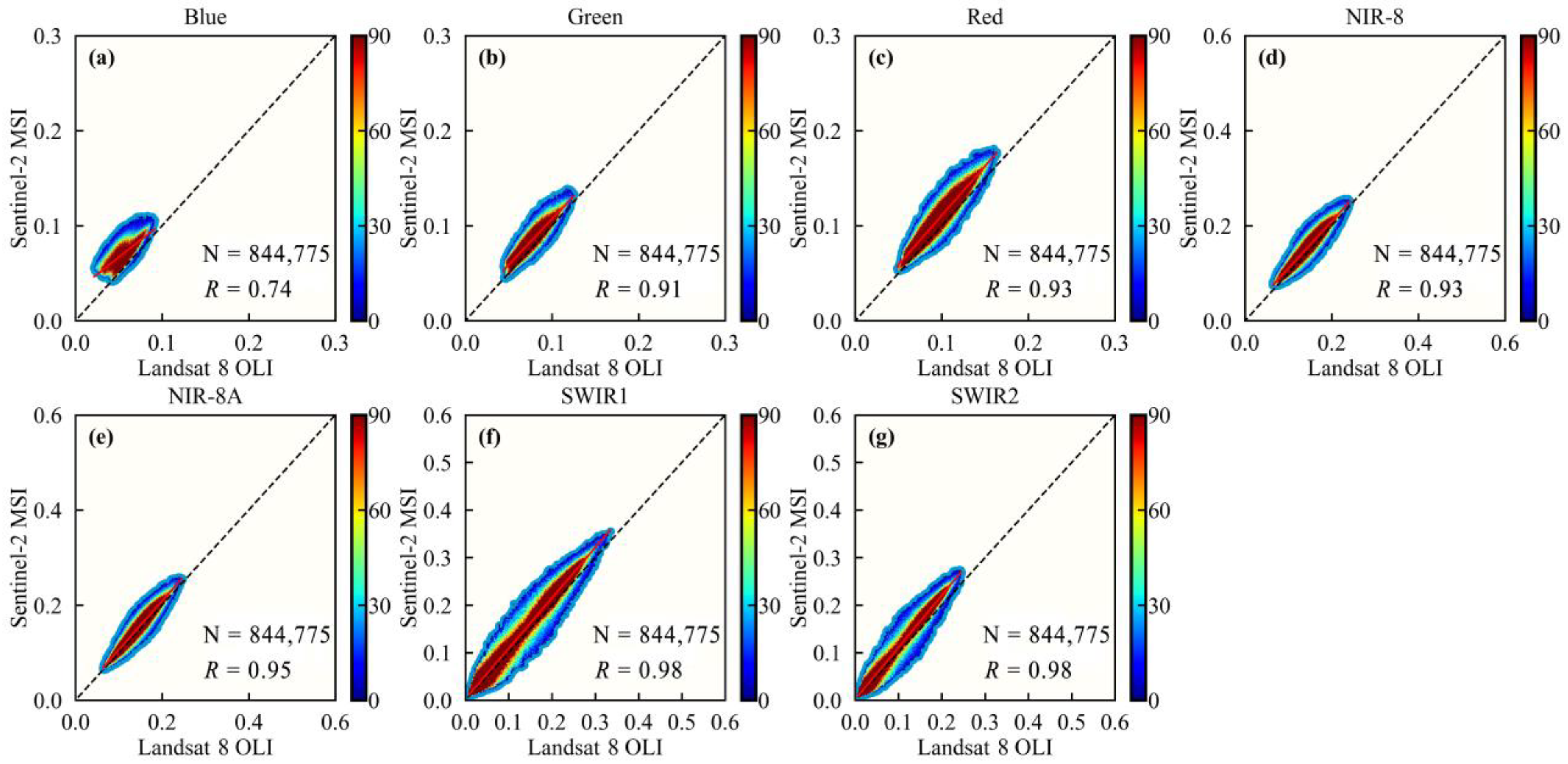
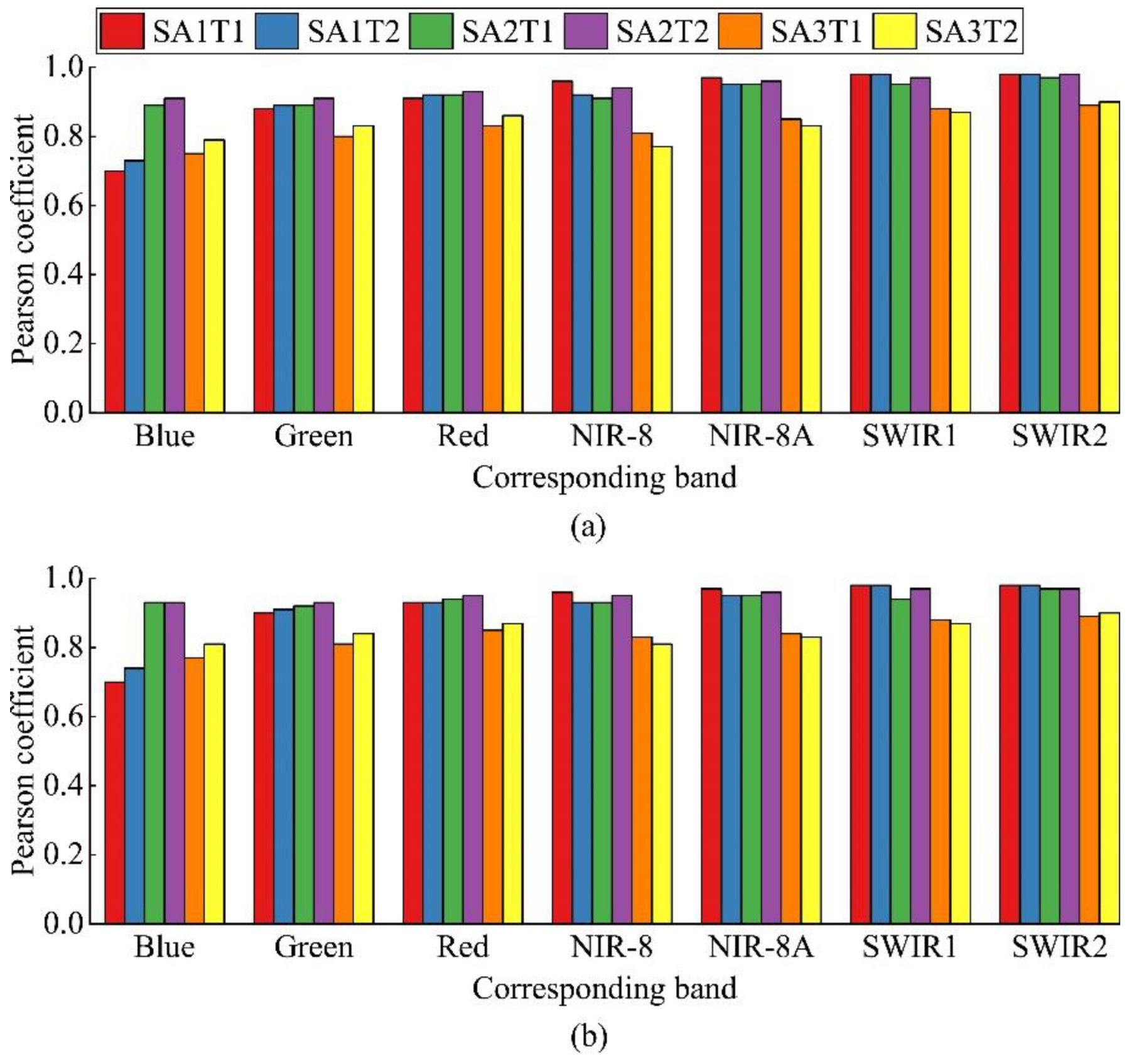
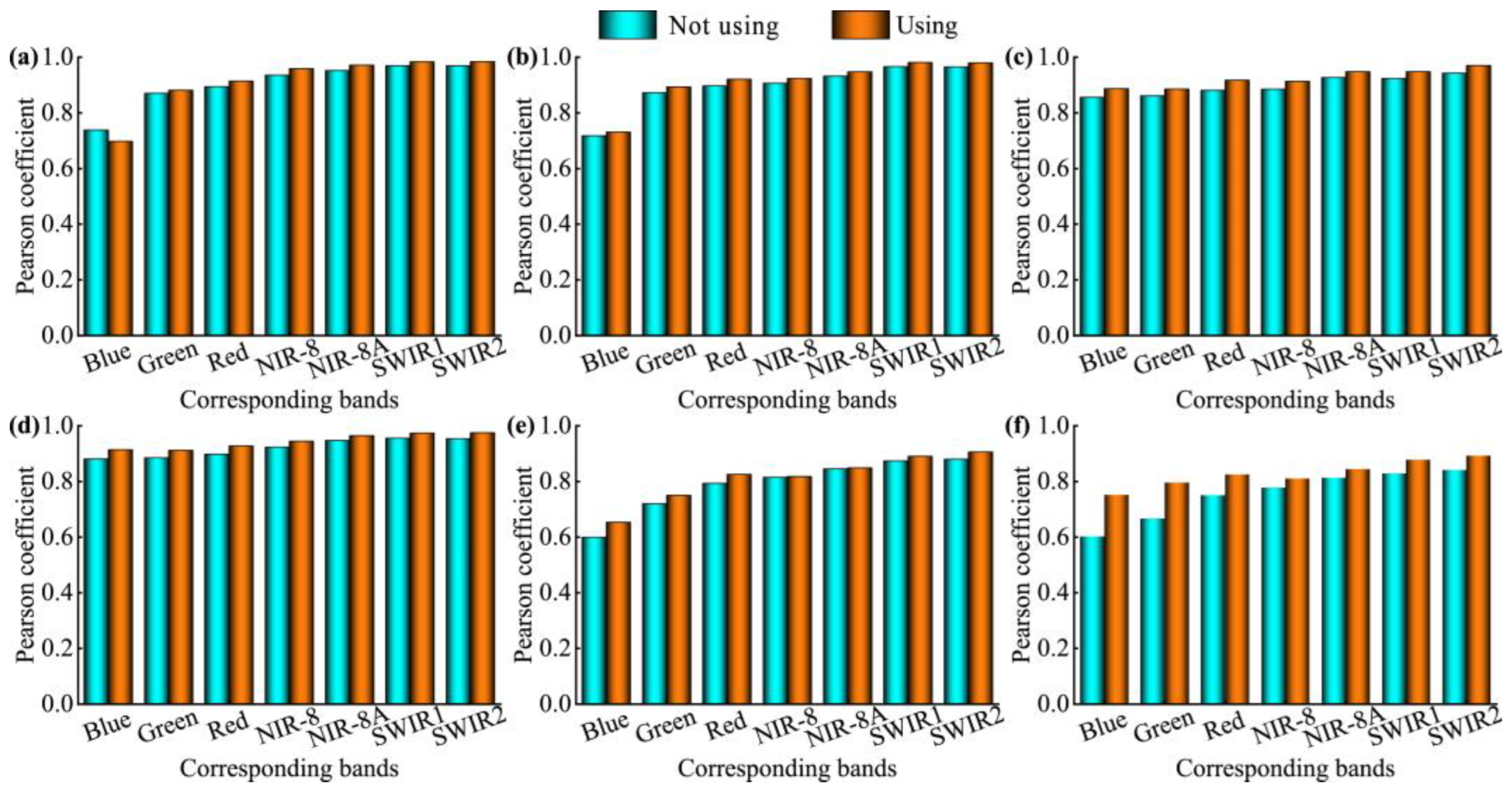
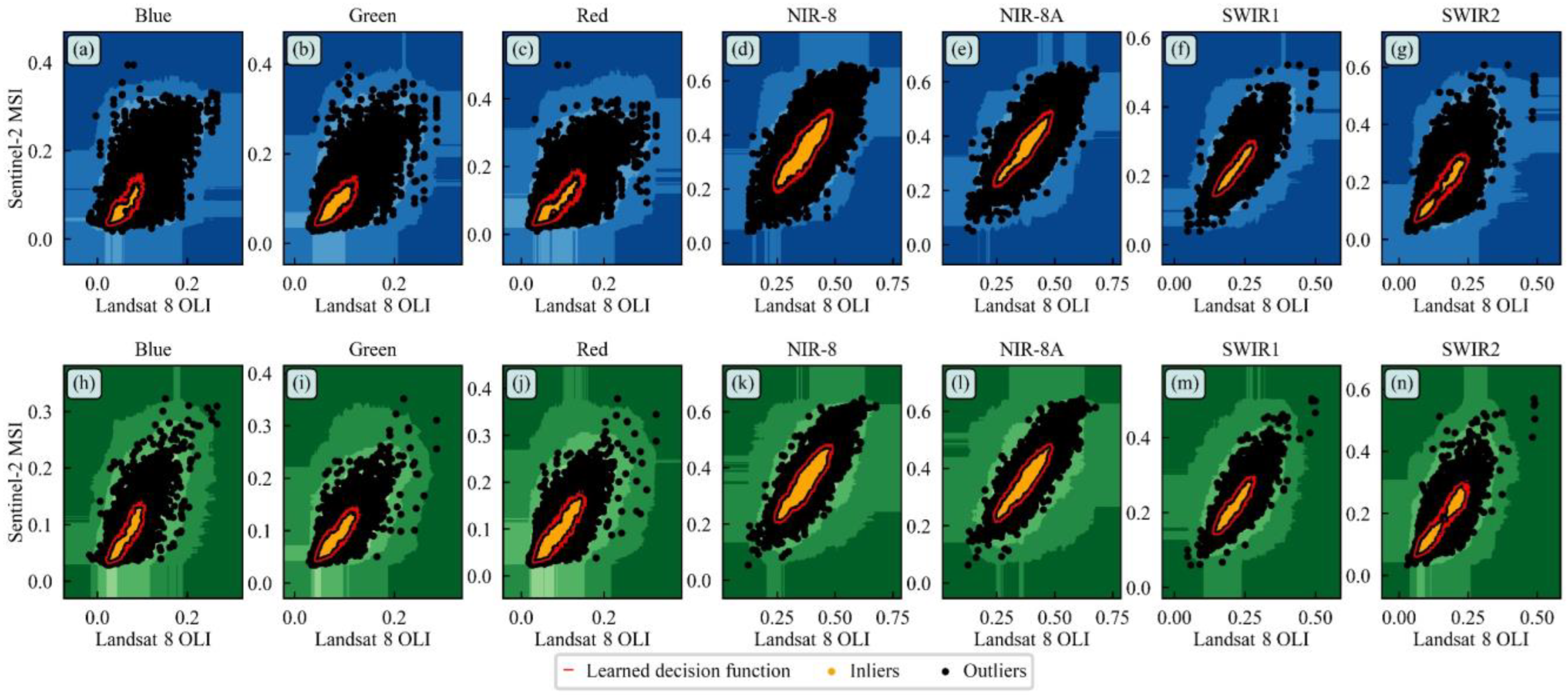
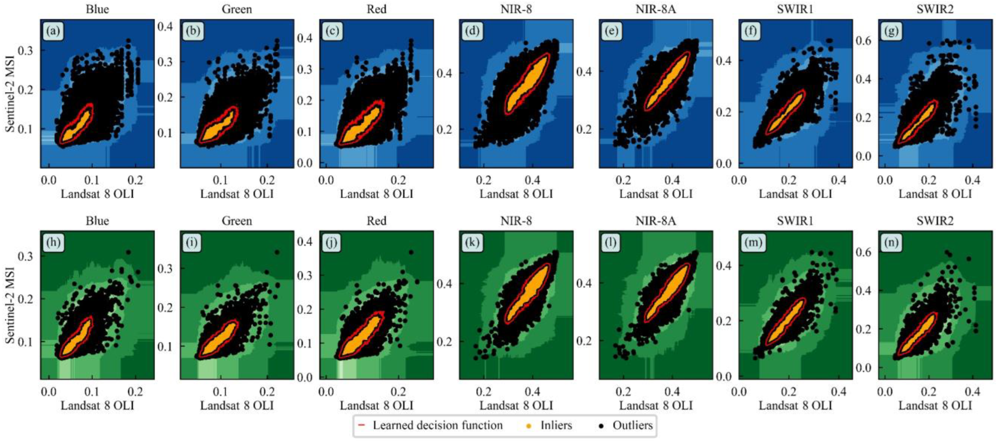
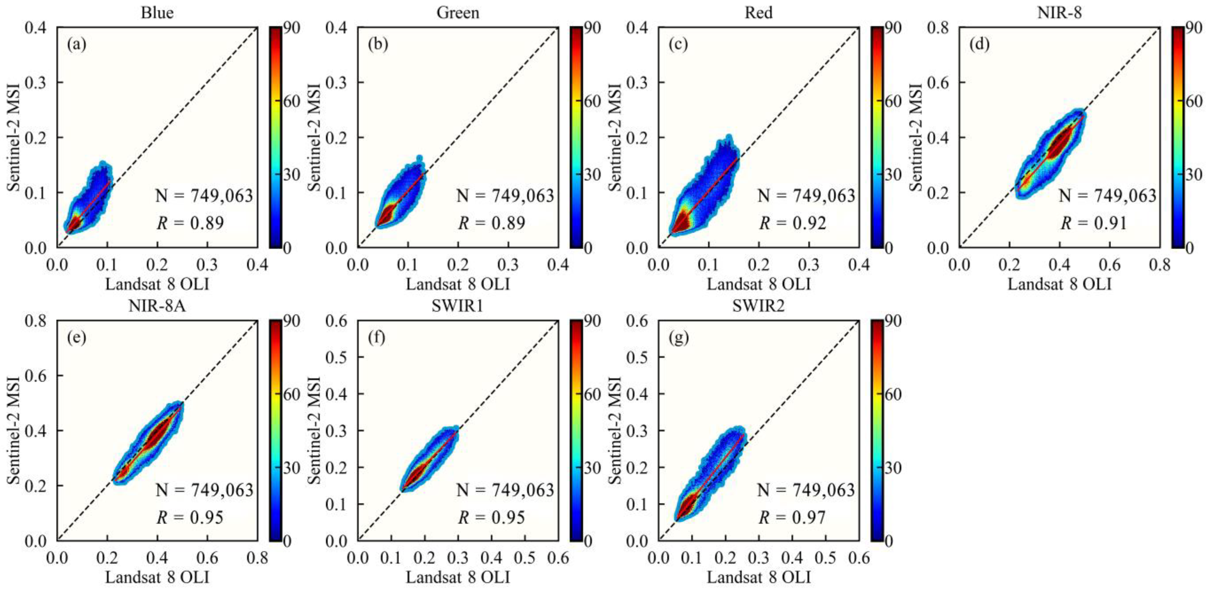
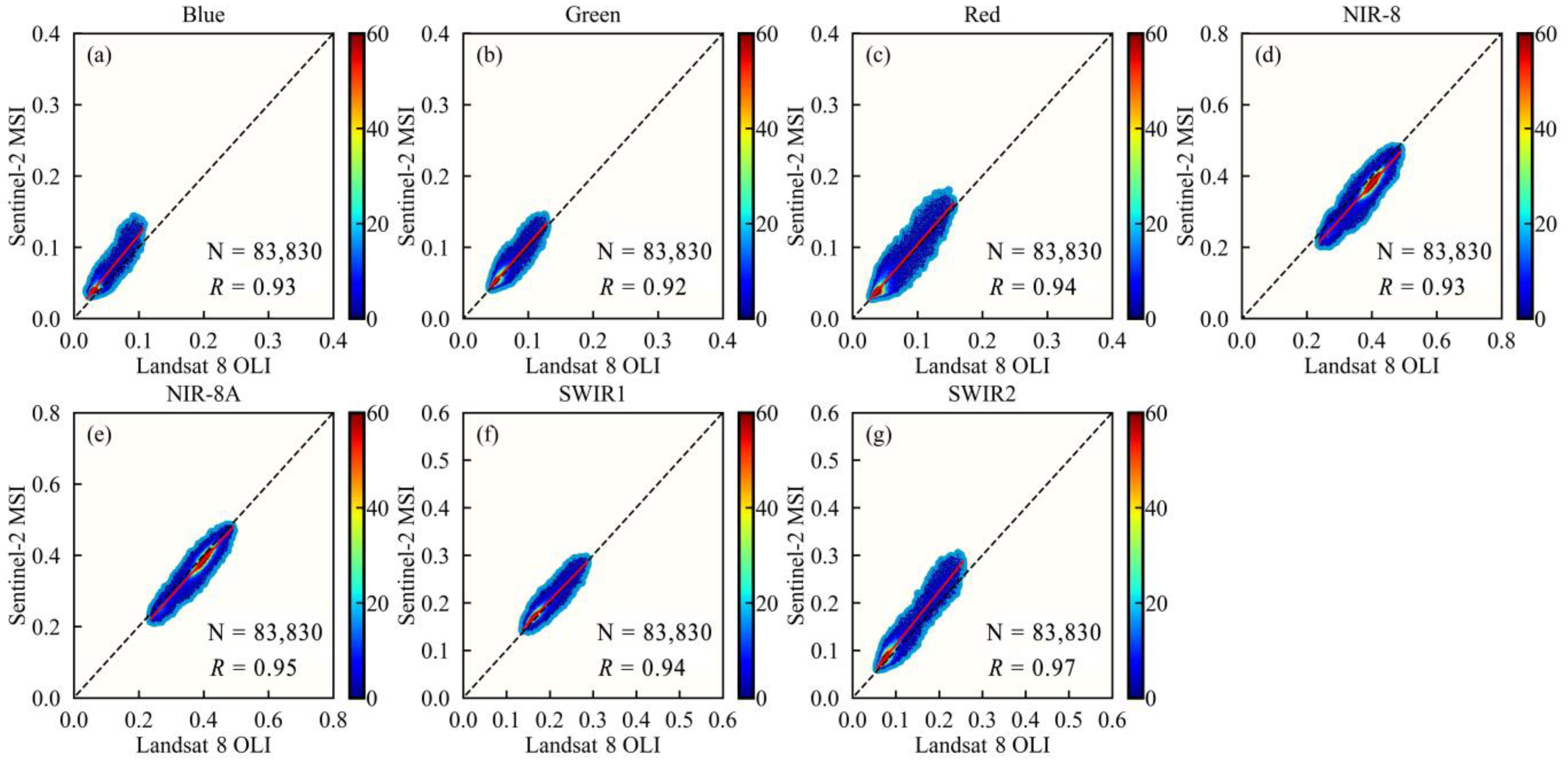
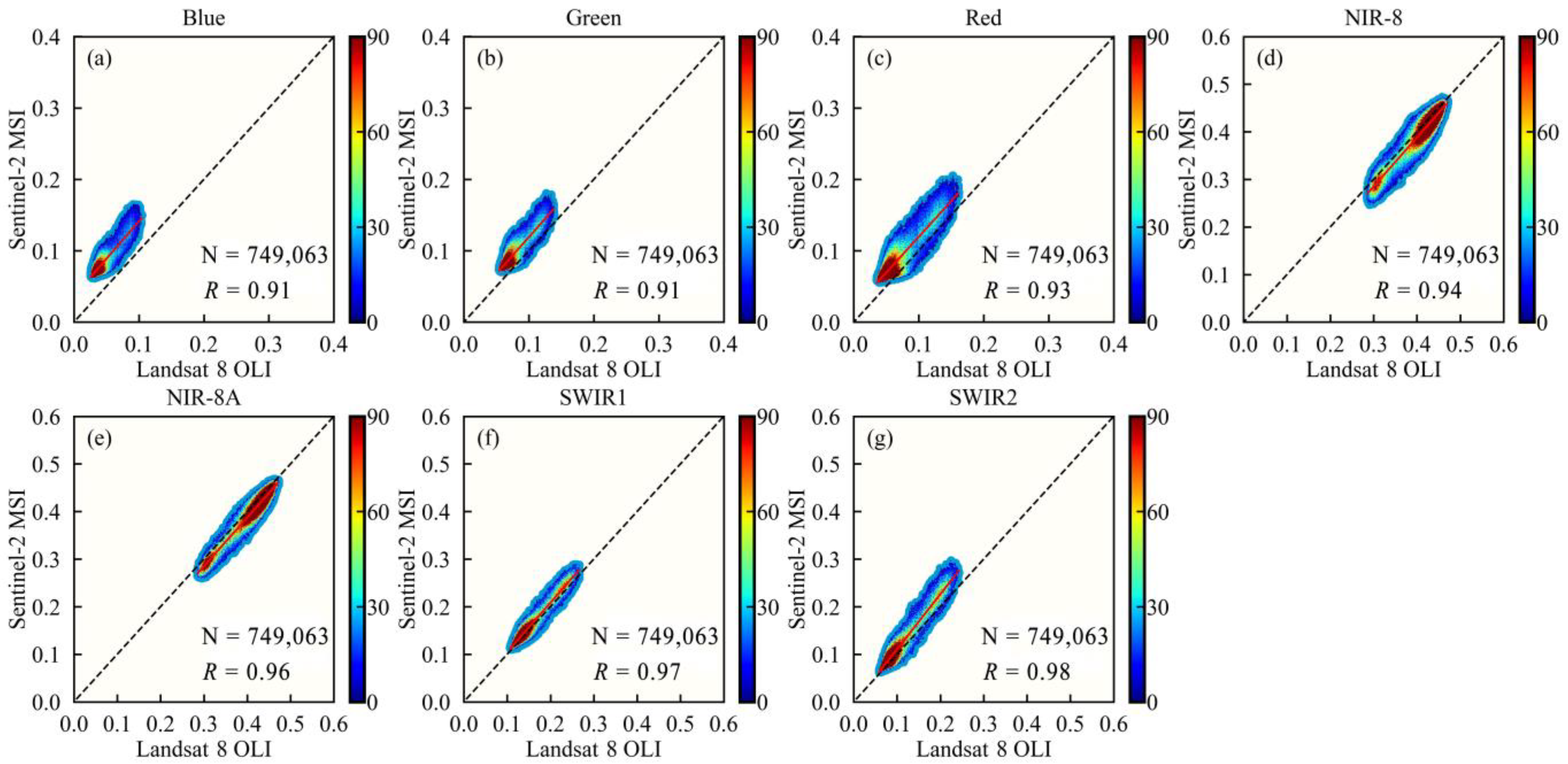
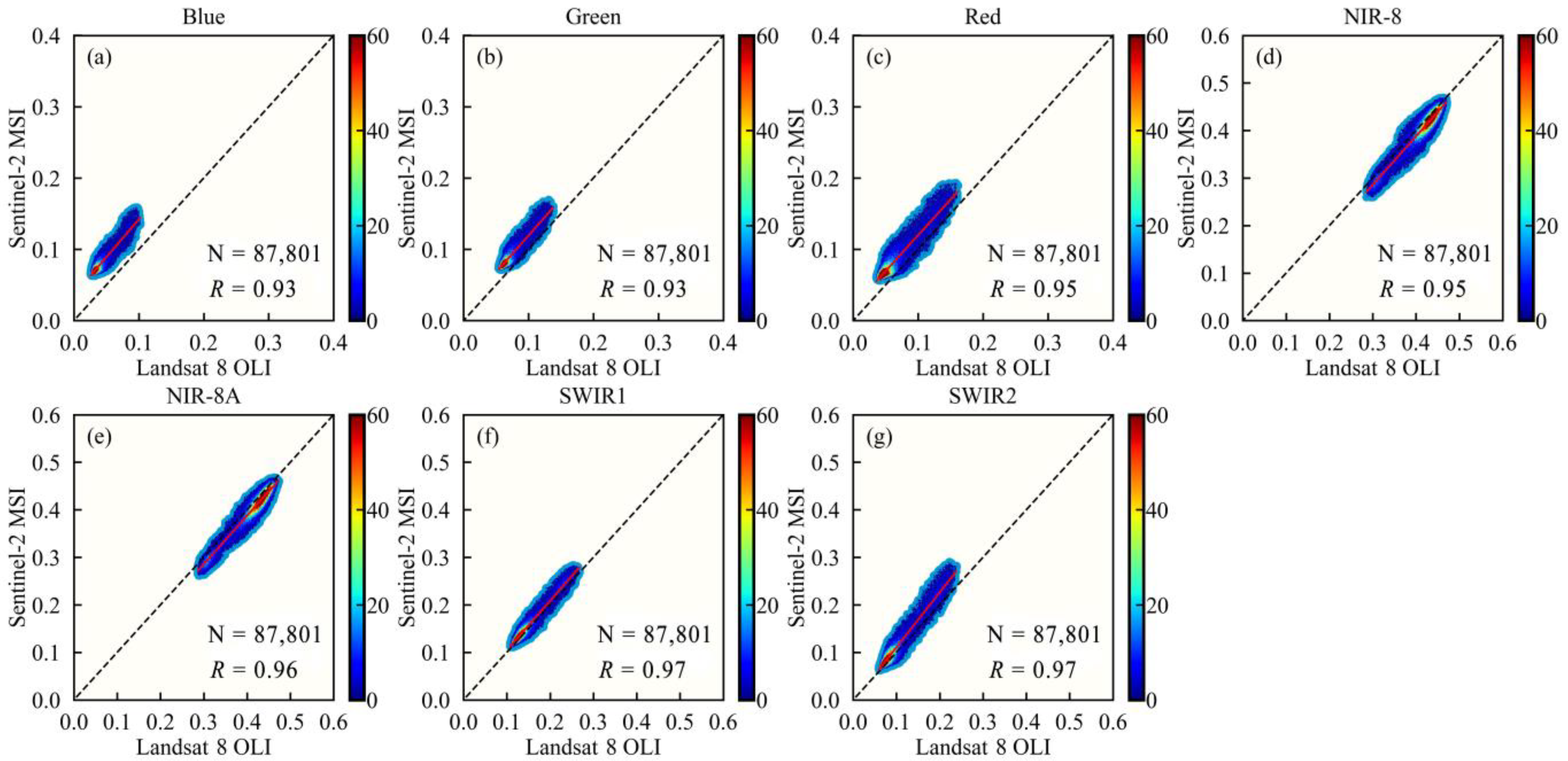
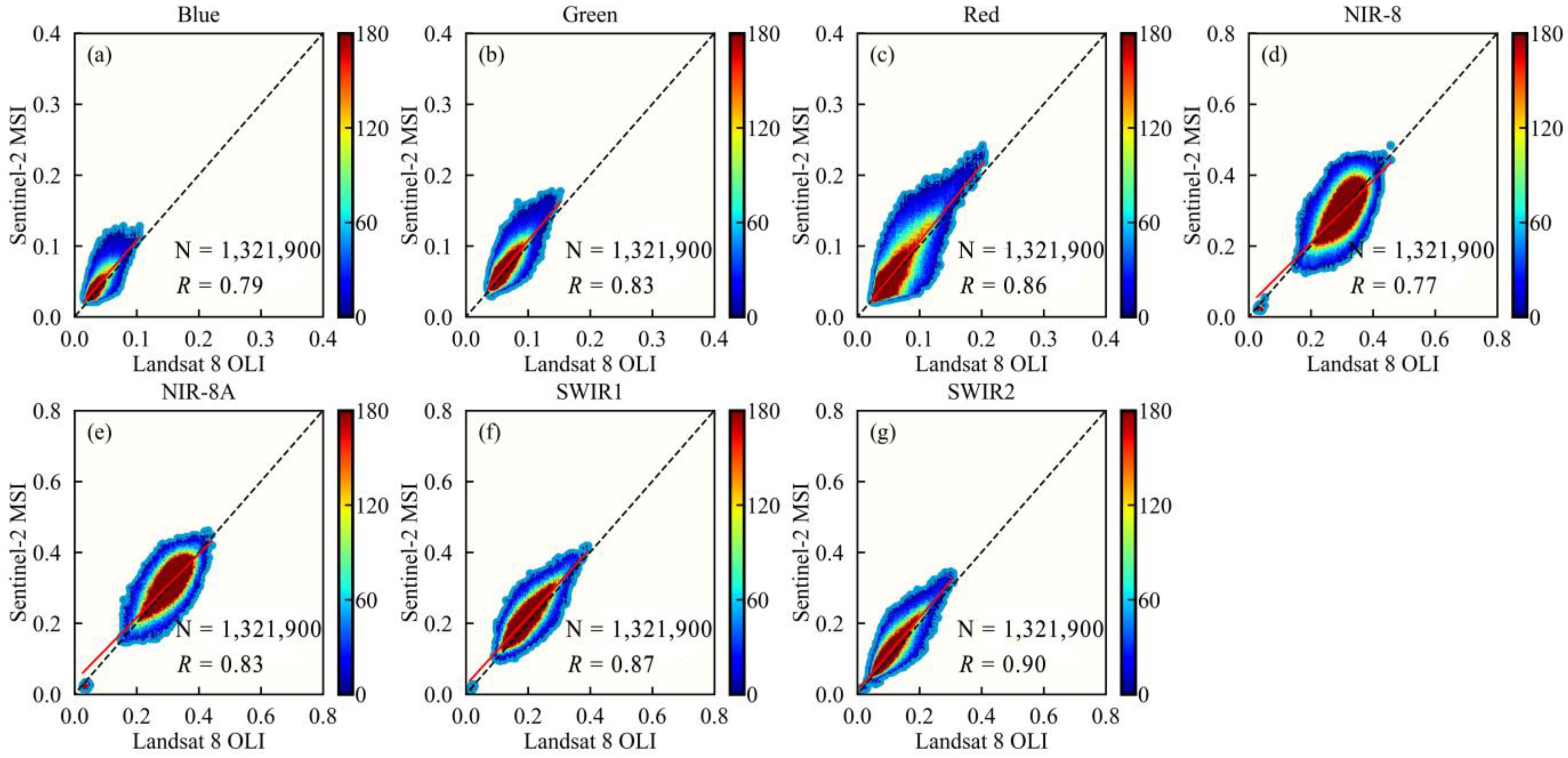
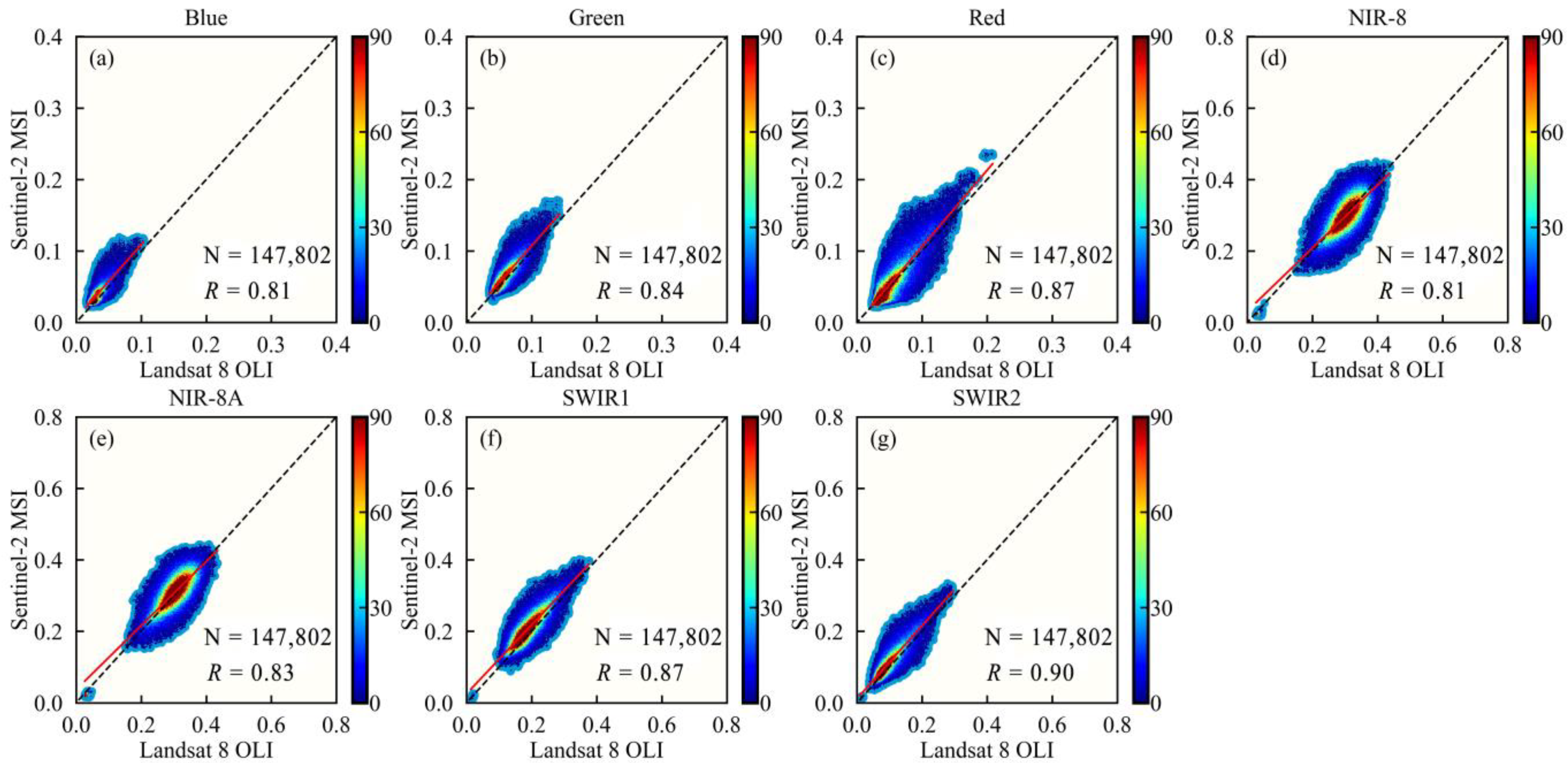
The implementation of the isolation forest algorithm proved effective in removing abnormal pixels from remote sensing images. This resulted in improved correlation between corresponding bands of Landsat 8 OLI and Sentinel-2 MSI sensors while reducing variations across farming areas at different latitudes. Notably, when both satellite images were resampled to a spatial resolution of 10 m, the correlation coefficients between corresponding bands consistently exceeded 0.88, indicating high radiometric consistency.
(2)
We employed a linear regression technique to linearly transform the six image pairs, encompassing high, middle, and low latitudes, thereby obtaining adjustment coefficients for integrating Landsat 8 OLI and Sentinel-2 data with high-spatial resolution at mixed latitudes. Through rigorous qualitative and quantitative analyses and a thorough examination of spatial heterogeneity, we have successfully verified the overall applicability of these adjustment factors, yielding highly satisfactory results.
(3)
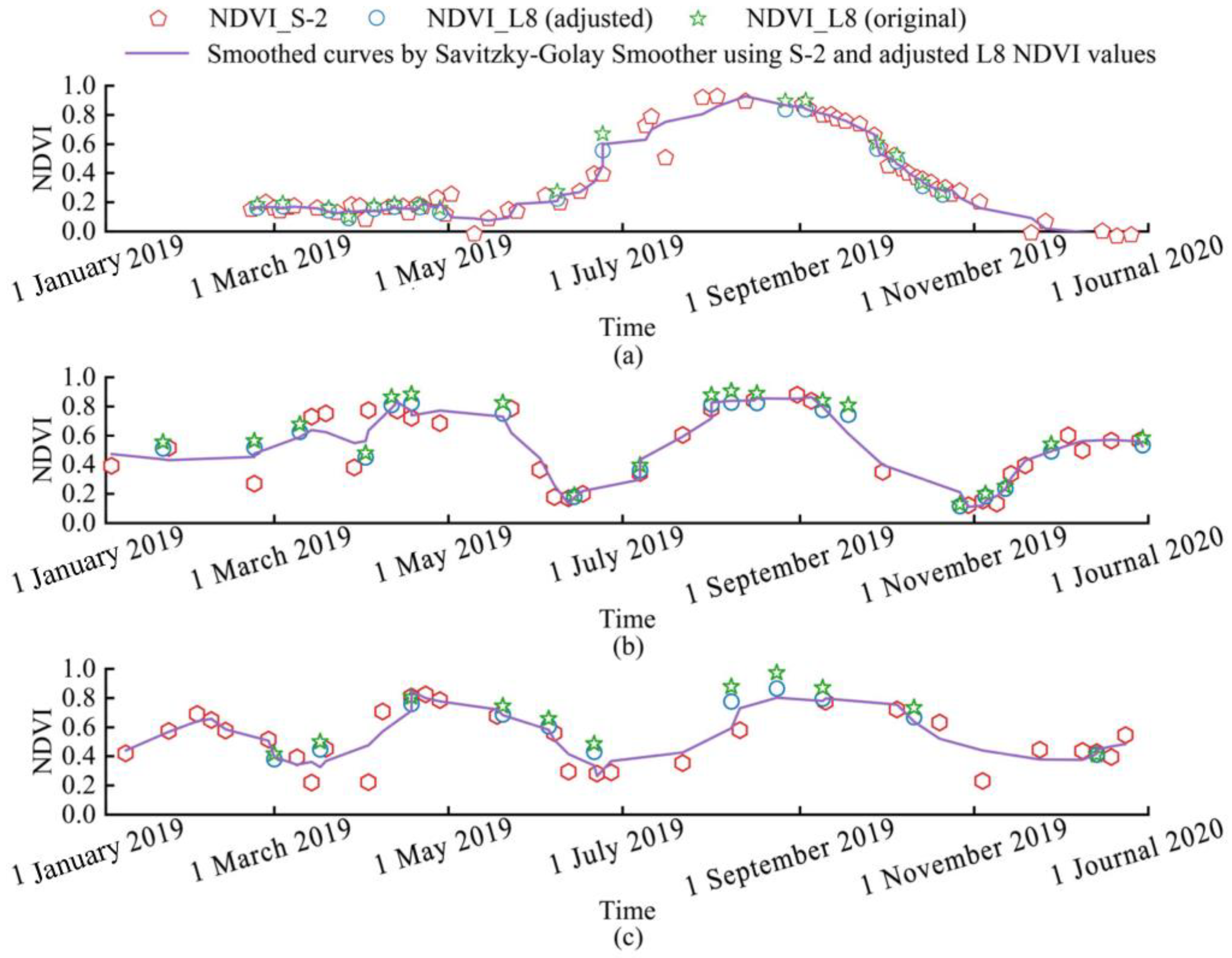
The application of the derived adjustment coefficients significantly improved monitoring density and accuracy in crop growth and development monitoring. Furthermore, the resulting NDVI time series accurately captured the intensity changes in crop growth status.

Author Contributions

Conceptualization, H.Z. and Y.Z.; methodology, H.Z.; software, S.L.; validation, H.Z. and T.G.; formal analysis, H.Z.; investigation, T.G.; resources, F.T.; data curation, F.T.; writing—original draft preparation, H.Z.; writing—review and editing, Y.Z.; visualization, S.L.; supervision, M.L.; project administration, M.L.; funding acquisition, Y.Z. and M.L. All authors have read and agreed to the published version of the manuscript.

Funding

This study was funded by the Smart Fertilization Project of China and the National Natural Science Foundation of China (41801245).

Data Availability Statement

Not applicable.

Conflicts of Interest

The authors declare no conflict of interest.

Appendix A

Figure A1. Processing results of the SA2T1 image pair using the isolation forest algorithm. (ag) have a blue background with 10 m spatial resolution, and (hn) have a green background with 30 m spatial resolution.
Remotesensing 15 02951 g0a1
Figure A2. Processing results of the SA2T2 image pair using the isolation forest algorithm. (ag) have a blue background with 10 m spatial resolution, and (hn) have a green background with 30 m spatial resolution.
Remotesensing 15 02951 g0a2
Figure A3. Processing results of the SA3T1 image pair using the isolation forest algorithm. (ag) have a blue background with 10 m spatial resolution, and (hn) have a green background with 30 m spatial resolution.
Remotesensing 15 02951 g0a3
Figure A4. Processing results of the SA3T2 image pair using the isolation forest algorithm. (ag) have a blue background with 10 m spatial resolution, and (hn) have a green background with 30 m spatial resolution.
Remotesensing 15 02951 g0a4
Figure A5. Scatterplots for the corresponding spectral bands of the SA2T1 image pair with 10 m spatial resolution were processed using the isolation forest algorithm. (ag) denote the scatterplots between the corresponding blue, green, red, NIR-8, NIR-8A, SWIR1 and SWIR2 bands of the S-2 and L8 sensors, respectively. The black dashed line is the 1:1 line; the red solid line is the OLS regression.
Remotesensing 15 02951 g0a5
Figure A6. Scatterplots for the corresponding spectral bands of the SA2T1 image pair with 30 m spatial resolution were processed using the isolation forest algorithm. (ag) denote the scatterplots between the corresponding blue, green, red, NIR-8, NIR-8A, SWIR1 and SWIR2 bands of the S-2 and L8 sensors, respectively. The black dashed line is the 1:1 line; the red solid line is the OLS regression.
Remotesensing 15 02951 g0a6
Figure A7. Scatterplots for the corresponding spectral bands of the SA2T2 image pair with 10 m spatial resolution were processed using the isolation forest algorithm. (ag) denote the scatterplots between the corresponding blue, green, red, NIR-8, NIR-8A, SWIR1 and SWIR2 bands of the S-2 and L8 sensors, respectively. The black dashed line is the 1:1 line; the red solid line is the OLS regression.
Remotesensing 15 02951 g0a7
Figure A8. Scatterplots for the corresponding spectral bands of the SA2T2 image pair with 30 m spatial resolution were processed using the isolation forest algorithm. (ag) denote the scatterplots between the corresponding blue, green, red, NIR-8, NIR-8A, SWIR1 and SWIR2 bands of the S-2 and L8 sensors, respectively. The black dashed line is the 1:1 line; the red solid line is the OLS regression.
Remotesensing 15 02951 g0a8
Figure A9. Scatterplots for the corresponding spectral bands of the SA3T1 image pair with 10 m spatial resolution were processed using the isolation forest algorithm. (ag) denote the scatterplots between the corresponding blue, green, red, NIR-8, NIR-8A, SWIR1 and SWIR2 bands of the S-2 and L8 sensors, respectively. The black dashed line is the 1:1 line; the red solid line is the OLS regression.
Remotesensing 15 02951 g0a9
Figure A10. Scatterplots for the corresponding spectral bands of the SA3T1 image pair with 30 m spatial resolution were processed using the isolation forest algorithm. (ag) denote the scatterplots between the corresponding blue, green, red, NIR-8, NIR-8A, SWIR1 and SWIR2 bands of the S-2 and L8 sensors, respectively. The black dashed line is the 1:1 line; the red solid line is the OLS regression.
Remotesensing 15 02951 g0a10
Figure A11. Scatterplots for the corresponding spectral bands of the SA3T2 image pair with 10 m spatial resolution were processed using the isolation forest algorithm. (ag) denote the scatterplots between the corresponding blue, green, red, NIR-8, NIR-8A, SWIR1 and SWIR2 bands of the S-2 and L8 sensors, respectively. The black dashed line is the 1:1 line; the red solid line is the OLS regression.
Remotesensing 15 02951 g0a11
Figure A12. Scatterplots for the corresponding spectral bands of the SA3T2 image pair with 30 m spatial resolution were processed using the isolation forest algorithm. (ag) denote the scatterplots between the corresponding blue, green, red, NIR-8, NIR-8A, SWIR1 and SWIR2 bands of the S-2 and L8 sensors, respectively. The black dashed line is the 1:1 line; the red solid line is the OLS regression.
Remotesensing 15 02951 g0a12

References

  1. Soriano-González, J.; Angelats, E.; Martínez-Eixarch, M.; Alcaraz, C. Monitoring Rice Crop and Yield Estimation with Sentinel-2 Data. Field. Crop. Res. 2022, 281, 108507. [Google Scholar] [CrossRef]
  2. Elmendorf, S.C.; Henry, G.H.; Hollister, R.D.; Björk, R.G.; Bjorkman, A.D.; Callaghan, T.V.; Collier, L.S.; Cooper, E.J.; Cornelissen, J.H.; Day, T.A. Global Assessment of Experimental Climate Warming on Tundra Vegetation: Heterogeneity over Space and Time. Ecol. Lett. 2012, 15, 164–175. [Google Scholar] [CrossRef] [PubMed]
  3. Roy, D.P.; Kovalskyy, V.; Zhang, H.K.; Vermote, E.F.; Yan, L.; Kumar, S.S.; Egorov, A. Characterization of Landsat-7 to Landsat-8 Reflective Wavelength and Normalized Difference Vegetation Index Continuity. Remote Sens. Environ. 2016, 185, 57–70. [Google Scholar] [CrossRef] [PubMed] [Green Version]
  4. Chen, Z.; Hao, P.; Liu, J.; An, M.; Han, B. Technical Demands of Agricultural Remote Sensing Satellites in China. Smart Agric. 2019, 1, 32–42. [Google Scholar]
  5. Shen, H.; Wu, J.; Cheng, Q.; Aihemaiti, M.; Zhang, C.; Li, Z. A Spatiotemporal Fusion Based Cloud Removal Method for Remote Sensing Images with Land Cover Changes. IEEE J. Sel. Top. Appl. Earth Obs. Remote Sens. 2019, 12, 862–874. [Google Scholar] [CrossRef]
  6. Shao, Z.; Pan, Y.; Diao, C.; Cai, J. Cloud Detection in Remote Sensing Images Based on Multiscale Features-Convolutional Neural Network. IEEE Trans. Geosci. Remote Sens. 2019, 57, 4062–4076. [Google Scholar] [CrossRef]
  7. Poortinga, A.; Tenneson, K.; Shapiro, A.; Nguyen, Q.; San Aung, K.; Chishtie, F.; Saah, D. Mapping Plantations in Myanmar by Fusing Landsat-8, Sentinel-2 and Sentinel-1 Data along with Systematic Error Quantification. Remote Sens. 2019, 11, 831. [Google Scholar] [CrossRef] [Green Version]
  8. Wulder, M.A.; Loveland, T.R.; Roy, D.P.; Crawford, C.J.; Masek, J.G.; Woodcock, C.E.; Allen, R.G.; Anderson, M.C.; Belward, A.S.; Cohen, W.B.; et al. Current Status of Landsat Program, Science, and Applications. Remote Sens. Environ. 2019, 225, 127–147. [Google Scholar] [CrossRef]
  9. Vermote, E.; Justice, C.; Claverie, M.; Franch, B. Preliminary Analysis of the Performance of the Landsat 8/OLI Land Surface Reflectance Product. Remote Sens. Environ. 2016, 185, 46–56. [Google Scholar] [CrossRef]
  10. Drusch, M.; Del Bello, U.; Carlier, S.; Colin, O.; Fernandez, V.; Gascon, F.; Hoersch, B.; Isola, C.; Laberinti, P.; Martimort, P.; et al. Sentinel-2: ESA’s Optical High-Resolution Mission for GMES Operational Services. Remote Sens. Environ. 2012, 120, 25–36. [Google Scholar] [CrossRef]
  11. Battude, M.; Al Bitar, A.; Morin, D.; Cros, J.; Huc, M.; Sicre, C.M.; Le Dantec, V.; Demarez, V. Estimating Maize Biomass and Yield over Large Areas Using High Spatial and Temporal Resolution Sentinel-2 like Remote Sensing Data. Remote Sens. Environ. 2016, 184, 668–681. [Google Scholar] [CrossRef]
  12. Rahman, M.M.; Robson, A. Integrating Landsat-8 and Sentinel-2 Time Series Data for Yield Prediction of Sugarcane Crops at the Block Level. Remote Sens. 2020, 12, 1313. [Google Scholar] [CrossRef] [Green Version]
  13. Bolton, D.K.; Gray, J.M.; Melaas, E.K.; Moon, M.; Eklundh, L.; Friedl, M.A. Continental-Scale Land Surface Phenology from Harmonized Landsat 8 and Sentinel-2 Imagery. Remote Sens. Environ. 2020, 240, 111685. [Google Scholar] [CrossRef]
  14. Flood, N. Comparing Sentinel-2A and Landsat 7 and 8 Using Surface Reflectance over Australia. Remote Sens. 2017, 9, 659. [Google Scholar] [CrossRef] [Green Version]
  15. Barsi, J.A.; Alhammoud, B.; Czapla-Myers, J.; Gascon, F.; Haque, M.O.; Kaewmanee, M.; Leigh, L.; Markham, B.L. Sentinel-2A MSI and Landsat-8 OLI Radiometric Cross Comparison over Desert Sites. Eur. J. Remote Sens. 2018, 51, 822–837. [Google Scholar] [CrossRef]
  16. Claverie, M.; Ju, J.; Masek, J.G.; Dungan, J.L.; Vermote, E.F.; Roger, J.-C.; Skakun, S.V.; Justice, C. The Harmonized Landsat and Sentinel-2 Surface Reflectance Data Set. Remote Sens. Environ. 2018, 219, 145–161. [Google Scholar] [CrossRef]
  17. Mandanici, E.; Bitelli, G. Preliminary Comparison of Sentinel-2 and Landsat 8 Imagery for a Combined Use. Remote Sens. 2016, 8, 1014. [Google Scholar] [CrossRef] [Green Version]
  18. Chastain, R.; Housman, I.; Goldstein, J.; Finco, M.; Tenneson, K. Empirical Cross Sensor Comparison of Sentinel-2A and 2B MSI, Landsat-8 OLI, and Landsat-7 ETM + Top of Atmosphere Spectral Characteristics over the Conterminous United States. Remote Sens. Environ. 2019, 221, 274–285. [Google Scholar] [CrossRef]
  19. Zhang, H.K.; Roy, D.P.; Yan, L.; Li, Z.; Huang, H.; Vermote, E.; Skakun, S.; Roger, J.-C. Characterization of Sentinel-2A and Landsat-8 Top of Atmosphere, Surface, and Nadir BRDF Adjusted Reflectance and NDVI Differences. Remote Sens. Environ. 2018, 215, 482–494. [Google Scholar] [CrossRef]
  20. Cao, H.; Han, L.; Li, L. Harmonizing surface reflectance between Landsat-7 ETM +, Landsat-8 OLI, and Sentinel-2 MSI over China. Environ. Sci. Pollut. Res. 2022, 29, 70882–70898. [Google Scholar] [CrossRef]
  21. Arekhi, M.; Goksel, C.; Sanli, F.B.; Senel, G. Comparative Evaluation of the Spectral and Spatial Consistency of Sentinel-2 and Landsat-8 OLI Data for Igneada Longos Forest. ISPRS. Int. J. Geo-Inf. 2019, 8, 56. [Google Scholar] [CrossRef] [Green Version]
  22. Chen, J.; Zhu, W. Comparing Landsat-8 and Sentinel-2 Top of Atmosphere and Surface Reflectance in High Latitude Regions: Case Study in Alaska. Geocarto. Int. 2022, 37, 6052–6071. [Google Scholar] [CrossRef]
  23. Atzberger, C. Advances in Remote Sensing of Agriculture: Context Description, Existing Operational Monitoring Systems and Major Information Needs. Remote Sens. 2013, 5, 949–981. [Google Scholar] [CrossRef] [Green Version]
  24. Wang, B.; Jia, K.; Wei, X.; Xia, M.; Yao, Y.; Zhang, X.; Liu, D.; Tao, G. Generating Spatiotemporally Consistent Fractional Vegetation Cover at Different Scales Using Spatiotemporal Fusion and Multiresolution Tree Methods. ISPRS J. Photogramm. 2020, 167, 214–229. [Google Scholar] [CrossRef]
  25. Guo, J.; Hu, Y. Spatiotemporal Variations in Satellite-Derived Vegetation Phenological Parameters in Northeast China. Remote Sens. 2022, 14, 705. [Google Scholar] [CrossRef]
  26. Meraner, A.; Ebel, P.; Zhu, X.X.; Schmitt, M. Cloud Removal in Sentinel-2 Imagery Using a Deep Residual Neural Network and SAR-Optical Data Fusion. ISPRS J. Photogramm. 2020, 166, 333–346. [Google Scholar] [CrossRef]
  27. Rembold, F.; Atzberger, C.; Savin, I.; Rojas, O. Using Low Resolution Satellite Imagery for Yield Prediction and Yield Anomaly Detection. Remote Sens. 2013, 5, 1704–1733. [Google Scholar] [CrossRef] [Green Version]
  28. Roy, D.P.; Wulder, M.A.; Loveland, T.R.; Woodcock, C.E.; Allen, R.G.; Anderson, M.C.; Helder, D.; Irons, J.R.; Johnson, D.M.; Kennedy, R.; et al. Landsat-8: Science and Product Vision for Terrestrial Global Change Research. Remote Sens. Environ. 2014, 145, 154–172. [Google Scholar] [CrossRef] [Green Version]
  29. Barsi, J.A.; Lee, K.; Kvaran, G.; Markham, B.L.; Pedelty, J.A. The Spectral Response of the Landsat-8 Operational Land Imager. Remote Sens. 2014, 6, 10232–10251. [Google Scholar] [CrossRef] [Green Version]
  30. Gorelick, N.; Hancher, M.; Dixon, M.; Ilyushchenko, S.; Thau, D.; Moore, R. Google Earth Engine: Planetary-scale Geospatial Analysis for Everyone. Remote Sens. Environ. 2017, 202, 18–27. [Google Scholar] [CrossRef]
  31. Veloso, A.; Mermoz, S.; Bouvet, A.; Thuy Le, T.; Planells, M.; Dejoux, J.-F.; Ceschia, E. Understanding the Temporal Behavior of Crops Using Sentinel-1 and Sentinel-2-Like Data for Agricultural Applications. Remote Sens. Environ. 2017, 199, 415–426. [Google Scholar] [CrossRef]
  32. Zheng, H.; Du, P.; Chen, J.; Xia, J.; Li, E.; Xu, Z.; Li, X.; Yokoya, N. Performance Evaluation of Downscaling Sentinel-2 Imagery for Land Use and Land Cover Classification by Spectral-Spatial Features. Remote Sens. 2017, 9, 1274. [Google Scholar] [CrossRef] [Green Version]
  33. Roy, D.P.; Zhang, H.K.; Ju, J.; Gomez-Dans, J.L.; Lewis, P.E.; Schaaf, C.B.; Sun, Q.; Li, J.; Huang, H.; Kovalskyy, V. A General Method to Normalize Landsat Reflectance Data to Nadir BRDF Adjusted Reflectance. Remote Sens. Environ. 2016, 176, 255–271. [Google Scholar] [CrossRef] [Green Version]
  34. Liu, F.T.; Ting, K.M.; Zhou, Z.-H. Isolation Forest. In Proceedings of the 8th IEEE International Conference on Data Mining, Pisa, Italy, 15–19 December 2008. [Google Scholar]
  35. Li, S.; Zhang, K.; Duan, P.; Kang, X. Hyperspectral Anomaly Detection with Kernel Isolation Forest. IEEE Trans. Geosci. Remote Sens. 2020, 58, 319–329. [Google Scholar] [CrossRef]
  36. Liu, D.; Zhen, H.; Kong, D.; Chen, X.; Zhang, L.; Yuan, M.; Wang, H. Sensors Anomaly Detection of Industrial Internet of Things Based on Isolated Forest Algorithm and Data Compression. Sci. Program. 2021, 2021, 6699313. [Google Scholar] [CrossRef]
  37. Zhang, Y.; Dong, Y.; Wu, K.; Chen, T. Hyperspectral Anomaly Detection with Otsu-Based Isolation Forest. IEEE J. Sel. Top. Appl. Earth Obs. Remote Sens. 2021, 14, 9079–9088. [Google Scholar] [CrossRef]
  38. Rzhetsky, A.; Nei, M. Statistical Properties of the Ordinary Least-Squares, Generalized Least-Squares, and Minimum-Evolution Methods of Phylogenetic Inference. J. Mol. Evol. 1992, 35, 367–375. [Google Scholar] [CrossRef]
  39. Zhang, X.; Lin, Q.; Xu, Y.; Qin, S.; Zhang, H.; Qiao, B.; Dang, Y.; Yang, X.; Cheng, Q.; Chintalapati, M. Cross-dataset Time Series Anomaly Detection for Cloud Systems. In Proceedings of the USENIX Annual Technical Conference, Renton, WA, USA, 30 September–2 October 2019; pp. 1063–1076. [Google Scholar]
  40. Landsat 8 Collection 1 Land Surface Reflectance Code Product Guide. Available online: https://www.usgs.gov/media/files/landsat-8-collection-1-land-surface-reflectance-code-product-guide (accessed on 21 October 2022).
  41. Schubert, E.; Sander, J.; Ester, M.; Kriegel, H.-P.; Xu, X. DBSCAN Revisited, Revisited: Why and How You Should (Still) Use DBSCAN. Acm. T. Database Syst. 2017, 42, 1–21. [Google Scholar] [CrossRef]
  42. Paulauskas, N.; Bagdonas, A.F. Local Outlier Factor Use for the Network Flow Anomaly Detection. Secur. Commun. Netw. 2015, 8, 4203–4212. [Google Scholar] [CrossRef] [Green Version]
  43. Claverie, M.; Masek, J.G.; Ju, J.; Dungan, J.L. Harmonized Landsat-8 Sentinel-2 (HLS) Product User’s Guide; National Aeronautics and Space Administration (NASA): Washington, DC, USA, 2017.
Figure 1. Location of the three study areas. The areas connected by the blue dotted line, the red dotted line, and the yellow dotted line are SA1, SA2, and SA3, respectively; the purple-filled pentagram indicates SA4.
Remotesensing 15 02951 g001
Figure 2. SRF curves of L8 OLI (green solid lines), S-2A MSI (blue dashed lines), and S-2B MSI (red dashed lines). (ag) denote blue, green, red, NIR, NIR-8A, SWIR1, and SWIR2 bands, respectively. The SRF curves for L8 OLI were obtained from the metadata provided by the United States Geological Survey at https://landsat.usgs.gov/spectral-characteristics-viewer (accessed on 15 September 2022), while the SRF curves for S-2A/B MSI were obtained using metadata information provided by the ESA at https://sentinels.copernicus.eu/web/sentinel/user-guides/sentinel-2-msi/document-library/-/asset_publisher/Wk0TKajiISaR/content/sentinel-2a-spectral-responses (accessed on 15 September 2022).
Remotesensing 15 02951 g002
Figure 3. RGB images of seven image pairs from L8 OLI and S-2A/B MSI for the four study areas (in the background images, the RGB composites are red, green, and blue). (a) indicates an S-2 MSI image on 10 June 2020; (b) represents an L8 OLI image on 10 June 2020; (c) denotes an S-2 MSI image with the time of 26 April 2021; (d) shows an L8 OLI image with the time of 26 April 2021; (e) represents a S-2 MSI image on 4 September 2020; (f) denotes a L8 OLI image on 4 September 2020; (g) indicates a S-2 MSI image with the time of 2 May 2021; (h) represents a L8 OLI image with the time of 2 May 2021; (i) shows a S-2 MSI image on 10 August 2020; (j) represents a L8 OLI image on 10 August 2020; (k) shows a S-2 MSI image on 3 December 2021; (l) indicates a L8 OLI image on 3 December 2021; (m) indicates S-2 MSI image with the time of 26 April 2021; (n) denotes a L8 OLI image with the time of 26 April 2021; (o) represents the S-2 image in the farmland scene at 10 m spatial resolution; (p) denotes the L8 image in the farmland scene at 30 m spatial resolution.
Remotesensing 15 02951 g003
Figure 4. Process for harmonized consistency analysis of L8 and S-2 sensor images.
Remotesensing 15 02951 g004
Figure 5. Processing results of the SA1T1 image pair using the iForest algorithm. (ag) have a blue background with 10 m spatial resolution, and (hn) have a green background with 30 m spatial resolution.
Remotesensing 15 02951 g005
Figure 6. Processing results of the SA1T2 image pair using the iForest algorithm. (ag) have a blue background with 10 m spatial resolution, and (hn) have a green background with 30 m spatial resolution.
Remotesensing 15 02951 g006
Figure 7. Scatterplots for the corresponding spectral bands of the SA1T1 image pair with 10 m spatial resolution were processed using the iForest algorithm. (ag) denote the scatterplots between the corresponding blue, green, red, NIR-8, NIR-8A, SWIR1 and SWIR2 bands of the S-2 and L 8 sensors, respectively. The black dashed line is the 1:1 line; the red solid line is the OLS regression.
Remotesensing 15 02951 g007
Figure 8. Scatterplots for the corresponding spectral bands of the SA1T1 image pair with 30 m spatial resolution were processed using the iForest algorithm. (ag) denote the scatterplots between the corresponding blue, green, red, NIR-8, NIR-8A, SWIR1 and SWIR2 bands of the S-2 and L 8 sensors, respectively. The black dashed line is the 1:1 line; the red solid line is the OLS regression.
Remotesensing 15 02951 g008
Figure 9. Scatterplots for the corresponding spectral bands of the SA1T2 image pair with 10 m spatial resolution were processed using the iForest algorithm. (ag) denote the scatterplots between the corresponding blue, green, red, NIR-8, NIR-8A, SWIR1 and SWIR2 bands of the S-2 and L 8 sensors, respectively. The black dashed line is the 1:1 line; the red solid line is the OLS regression.
Remotesensing 15 02951 g009
Figure 10. Scatterplots for the corresponding spectral bands of the SA1T2 image pair with 30 m spatial resolution were processed using the iForest algorithm. (ag) denote the scatterplots between the corresponding blue, green, red, NIR-8, NIR-8A, SWIR1 and SWIR2 bands of the S-2 and L 8 sensors, respectively. The black dashed line is the 1:1 line; the red solid line is the OLS regression.
Remotesensing 15 02951 g010
Figure 11. Corresponding spectral band relationships of L8 OLI and S-2 MSI after processing with the iForest algorithm. (a) Indicates 10 m spatial resolution, and (b) represents 30 m spatial resolution.
Remotesensing 15 02951 g011
Figure 12. Scatterplots for the corresponding spectral bands of L8 OLI and S-2 MSI sensors with 10 m spatial resolution were processed using the iForest algorithm. (ag) denote the scatterplots between the corresponding blue, green, red, NIR-8, NIR-8A, SWIR1 and SWIR2 bands of the S-2 and L 8 sensors, respectively. The black dashed line is the 1:1 line; the red solid line is the OLS regression.
Remotesensing 15 02951 g012
Figure 13. NDVI time series curves for three-pixel sites using the integrated L8 and S-2 images. The red unfilled pentagon, blue unfilled circle, and green unfilled pentagram indicate the NDVI valves of S-2, adjusted L8, and original L8 images, respectively, and the purple lines represent the Smoothed curves by Savitzky-Golay Smoother using S-2 and adjusted L8 NDVI values. The pixel site locations of (ac) are 134.1276°E, 47.7272°N (SA1), 114.3339°E, 35.1436°N (SA2), and 109.30203°E, 19.62935°N (SA3).
Remotesensing 15 02951 g013
Figure 14. Comparison of correlation coefficients between L8 OLI and S-2 MSI sensors using and not using the iForest algorithm for the corresponding spectral bands. (a) represents an image pair on SA1T1; (b) indicates an image pair on SA1T2; (c) represents an image pair on SA2T1; (d) denotes an image pair on SA2T2; (e) indicates an image pair on SA3T1; (f) represents an image pair on SA3T2.
Remotesensing 15 02951 g014
Table 1. Comparison of spatial resolution, central wavelength, and bandwidth between the corresponding bands of S-2A MSI, S-2B MSI, and L8 OLI. The bandwidth in the tables below represents the values measured at Full Width Half Maximum (FWHM). (S-2A and S-2B MSI sensors are acquired at https://sentinels.copernicus.eu/web/sentinel/user-guides/sentinel-2-msi/resolutions/spectral (accessed on 26 September 2022), and the L8 OLI sensor is available at https://landsat.gsfc.nasa.gov/satellites/landsat-8/landsat-8-bands/ (accessed on 26 September 2022)).
SensorMeasureBlueGreenRedNIR-8NIR-8ASWIR1SWIR2
S-2A MSISpatial resolution (m)10101010202020
Central wavelength (nm)492.7559.8664.6832.8864.71613.72202.4
Bandwidth (nm)6535301052190174
S-2B MSISpatial resolution (m)10101010202020
Central wavelength (nm)492.3558.9664.9832.9864.01610.42185.7
Bandwidth (nm)6536311042194184
L8 OLISpatial resolution (m)303030-303030
Central wavelength (nm)482561655-86516092201
Bandwidth (nm)656040-3085190
Table 2. The Coordinated Universal Time (UTC), solar zenith angle, and solar azimuth angle for seven image pairs of L8 OLI and S-2A/B MSI.
Study AreaDate (Day-Month-Year)Satellite SensorsTime (UTC)Solar Zenith Angle (°)Solar Azimuth Angle (°)
SA110 June 2020S-2A MSI01:56:5926.91149.71
L8 OLI01:49:1928.29143.44
26 April 2021S-2A MSI02:00:1535.78156.29
L8 OLI01:49:1936.92150.86
SA24 September 2020S-2B MSI03:17:4731.29148.58
L8 OLI02:55:1733.63140.22
2 May 2021S-2B MSI03:17:4723.72140.60
L8 OLI02:54:3826.68130.86
SA310 August 2020S-2A MSI03:20:2120.4397.84
L8 OLI03:05:1524.4397.17
3 December 2021S-2A MSI03:11:0944.77157.18
L8 OLI03:05:3847.14152.79
SA426 April 2021S-2A MSI03:38:5022.62127.25
L8 OLI03:33:2325.47122.32
Table 3. Adjustment coefficients for L8 OLI and S-2 MSI sensors at mixed latitudes with 10 m spatial resolution.
CoefficientBlueGreenRedNIR-8NIR-8ASWIR1SWIR2
Slope0.78021.02931.09120.91980.95391.05551.0810
Intercept0.02040.00610.00010.01860.01550.00520.0049
Table 4. Test results of the adjustment coefficients derived for integrated L8 and S-2 data at high, middle, and low latitudes, respectively.
Study AreaIndexBands
BlueGreenRedNIR-8NIR-8ASWIR1SWIR2
SA1RMSE0.0120.0080.0110.0180.0140.0230.019
MAE0.0090.0060.0080.0130.0100.0140.011
SA2RMSE0.0140.0160.0210.0190.0170.0130.015
MAE0.0100.0130.0170.0140.0130.0100.010
SA3RMSE0.0170.0190.0250.0660.0670.0470.024
MAE0.0110.0110.0150.0440.0480.0290.013
Table 5. Test results for the spatial heterogeneity of the adjustment coefficients derived from integrated L8 and S-2 data.
IndexBands
BlueGreenRedNIR-8NIR-8ASWIR1SWIR2
RMSE0.0180.0170.0230.0460.0420.0220.020
MAE0.0120.0120.0160.0320.0290.0130.011
Table 6. Comparison of the conversion coefficients of the HLS product and the product in this paper.
ProductDirection of AdjustmentSpatial ResolutionCoefficientBlueGreenRedNIR-8NIR-8ASWIR1SWIR2
HLSL8 OLI from S-2 MSI30 mSlope1.0051.0200.9941.0170.9990.9991.003
Intercept2.09 × 10−44.47× 10³1.09 × 10³−1.04 × 10³2.50 × 10−41.24 × 10−41.19 × 10³
This articleS-2 MSI from L8 OLI10 mSlope0.85271.07331.14040.90240.93111.04161.1116
Intercept0.01860.0027−0.00250.01990.01630.00320.0013
Disclaimer/Publisher’s Note: The statements, opinions and data contained in all publications are solely those of the individual author(s) and contributor(s) and not of MDPI and/or the editor(s). MDPI and/or the editor(s) disclaim responsibility for any injury to people or property resulting from any ideas, methods, instructions or products referred to in the content.

