Article

Trade-Off and Synergy Relationships and Spatial Bundle Analysis of Ecosystem Services in the Qilian Mountains

1
Center for Glacier and Desert Research, Scientific Observing Station for Desert and Glacier, College of Earth and Environmental Sciences, Lanzhou University, Lanzhou 730000, China
2
Qinghai Province Institute of Meteorological Sciences, Xining 810001, China
3
College of History and Culture, Northwest Normal University, Lanzhou 730070, China
*
Author to whom correspondence should be addressed.
Remote Sens. 2023, 15(11), 2950; https://doi.org/10.3390/rs15112950
Submission received: 28 March 2023 / Revised: 27 May 2023 / Accepted: 3 June 2023 / Published: 5 June 2023

Abstract

:
Significant heterogeneity has been observed among different ecosystem services (ES). Understanding the trade-offs and synergies among ES and delineating ecological functional zones is crucial for formulating regional management policies that improve human well-being and sustainably develop and maintain ecosystems. In this study, we used the Integrated Valuation of Ecosystem Services and Trade-offs (InVEST) and Carnegie–Ames–Stanford Approach (CASA) models to evaluate the spatial distribution patterns of nine ES (food supply, raw material supply, water resource supply, water connotation, climate regulation, soil conservation, water purification, habitat quality, and entertainment tourism) in the Qilian Mountains from 2000 to 2018. We also investigated the trade-offs and synergistic relationships among ES through Spearman correlation analysis, identified ES hotspots through exploratory spatial data analysis, and identified ES bundles (ESB) using K-means clustering. Our results revealed that water purification and habitat quality remained relatively stable, while food supply, raw material supply, water resource supply, water conservation, climate regulation, soil conservation, and entertainment tourism increased by 1038.83 Yuan·ha−1, 448.21 Yuan·ha−1, 55.45 mm, 7.80 mm, 0.60 tc·ha−1, 40.01 t·ha−1 and 4.82, respectively. High-value areas for water resource supply were mainly concentrated in the high-altitude mountainous area, whereas high-value areas for soil conservation were found in the western and eastern parts of the study area. The low-value areas of water purification were primarily located in the east, while the remaining six services were highly distributed in the east and were less common in the west. Correlation analysis showed that water resource supply, water conservation, and soil conservation exhibited a synergistic relationship in the Qilian Mountains. Moreover, food supply, raw material supply, climate regulation, habitat quality, and entertainment tourism showed synergistic relationships. However, there were trade-offs between food supply and water purification as well as water resource supply, and habitat quality showed a tradeoff with water resource supply, water conservation, and soil conservation. We identified four ESB. The food supply bundle consisted mainly of farmland ecosystems, while the windbreak and sand fixation and ecological coordination bundles were dominant in the Qilian Mountains. Notably, the area of the water conservation bundle increased significantly. Our comprehensive findings on ES and ESB can provide a theoretical foundation for the formulation of ecological management policies and the sustainable development of ecosystems in the Qilian Mountains.

1. Introduction

Ecosystem services (ES) refer to the benefits and welfare that ecosystems provide to humans [1]. In 2005, the Millennium Ecosystem Assessment report, released by the United Nations, highlighted that 60% of the world’s ecosystems are in a degraded state [2]. Consequently, ES have become a significant focus of research in ecology and related disciplines [3,4]. Given the complexity and diversity of ES, the evident spatial heterogeneity in their distribution, and the fact that humans utilize ES to improve their own well-being, there exit complex linear and nonlinear relationships among ES [5]. Previous studies have categorized the relationship between ecosystems as trade-offs, synergies, and non-response [6]. In recent years, exploring the trade-off and synergy between ES has become a core issue in ES research [7,8,9,10]. If the evaluation of services provided by land is insufficient, then the one-sided pursuit of service while ignoring another type of service will lead to trade-offs, eventually resulting in the degradation of the ecological environment on a large scale [11]. Differences in climate, upper soil, and vegetation cover can make land-use types spatially heterogeneous, thus affecting ES [12]. Water resources play a crucial role in connecting and controlling different ecosystems while ensuring a stable water supply is essential for maintaining the stability of ES in a region [13]. Climate change significantly impacts the global water cycle, leading to changes in precipitation, evapotranspiration, and runoff patterns, altering the spatial and temporal distribution of water resources, and increasing the frequency of extreme disasters such as droughts and floods [14], and thus exacerbating the conflict between supply and demand of ES. Scholars from many countries, at regional [15,16,17,18], watershed [19,20,21], and other scales, have studied the trade-offs and synergies between ES and spatial-temporal differentiation characteristics [12,16,17,18,21,22,23]. However, most previous research focused only on several important services [15,22], with limited exploration of the relationships between provisioning, regulating, habitat, and cultural services. Additionally, there is a lack of research on the spatial composition of ES.
In recent years, the concept of ES bundles (ESB) has emerged to enhance the management of multifunctional landscapes [24]. ESB involves clustering ES to identify dominant services in a specific region, thereby improving ecosystem management by promoting synergies and reducing trade-offs. ESB represents combinations of services within a particular time and space, offering insights into the interdependent relationships among ES. Based on the similarity principle of clustering analysis, it can spatially quantify the composition and structure of ES and is a valuable tool for the identification of several important services in a study area [25,26]. Common methods used to identify service bundles include principal component analysis [26], self-organizing maps [25,27,28], spectral clustering, and k-means clustering analysis [29]. Current research on service bundles is mostly focused on different scales, such as countries [30], regions [31], and basins [32]. While these scales facilitate zoning management, they may not be optimal for studying services based on ecological processes. For fine-scale land management and research on services, it is beneficial to partition the study area into appropriate grids. However, there is currently a lack of research on the dynamic partitioning of ESB at the grid scale [33]. Therefore, using service bundles to study the spatial dynamic evolution of ES on a grid scale is of great significance for maintaining the sustainable development of ecosystems and providing targeted scientific decision-making, considering local economic development.
In the global terrestrial ecosystem, mountainous areas form approximately one-fourth of the total surface area; 12% of the global population lives in mountainous areas, and these areas are hot spots for more than 50% of the world’s plant and animal species [34]. The Qilian Mountains are an important water-producing area and a priority biodiversity conservation area in China. In addition, the ecological environment of these mountains is fragile and has drawn the attention of the societal community. The ecological protection of the Qilian Mountains is related to the ecological security and sustainable social development of Western China.
In view of this, we selected the Qilian Mountains as a representative case to investigate spatiotemporal changes and hotspots of ES, trade-offs, and synergies among ES and identify four distinct types of ecosystem service clusters. By integrating these findings with a decision support system, our research provides a valuable reference for future decision-making optimization and institutional reform of Qilian Mountain.

2. Materials and Methods
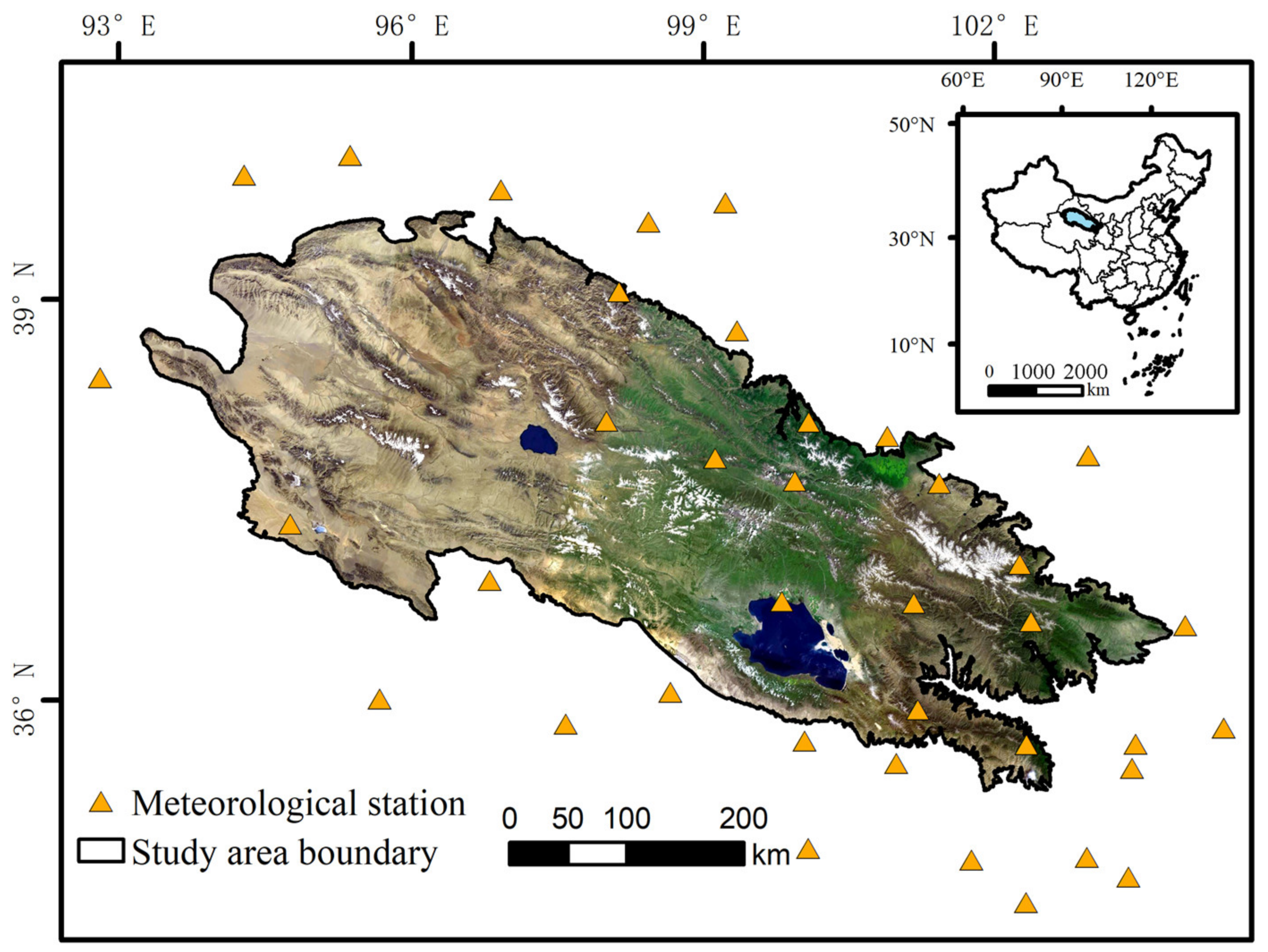
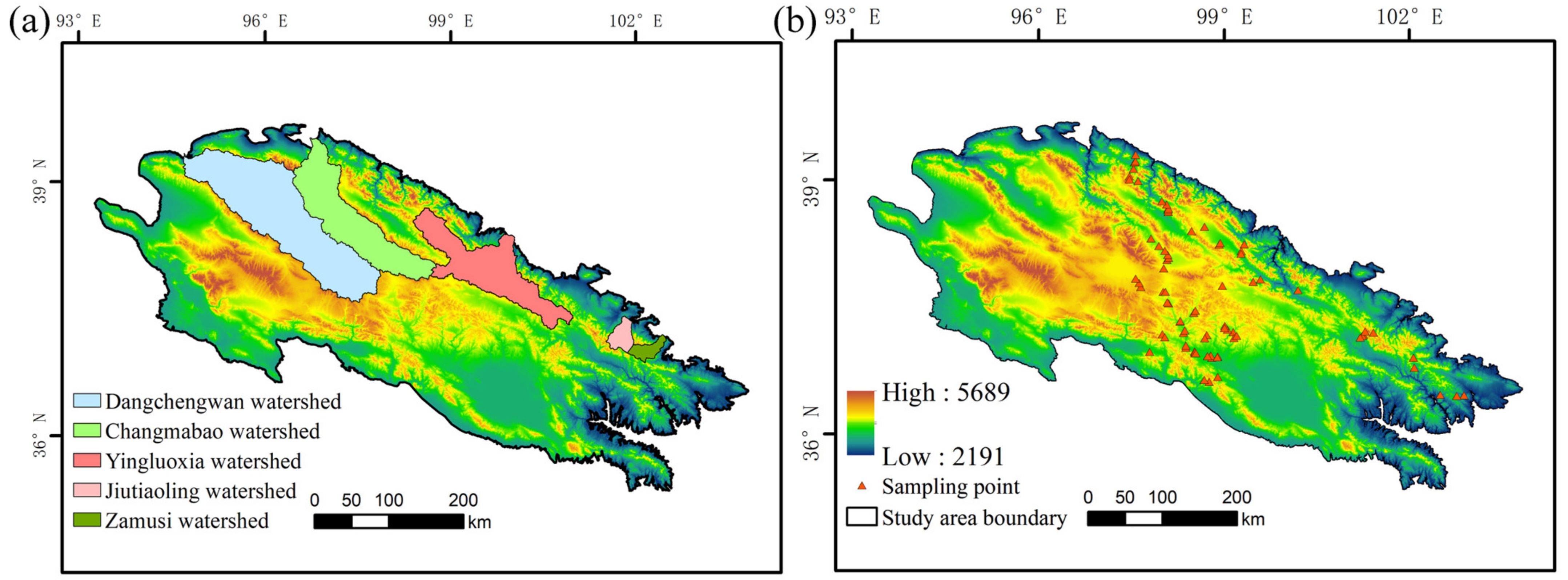
2.1. Study Area

The Qilian Mountain range is located in the arid and semi-arid inland region of northwest China at the intersection of the Qinghai–Tibet Plateau, Inner Mongolia Plateau, and Loess Plateau. It spans the Gansu and Qinghai provinces and is the largest marginal mountain system in the northeastern Qinghai–Tibet Plateau. Tuanjie Peak, the highest peak of Mountain Shulenan, is 5808 m above sea level [35,36]. Starting from Wushaoling in the east and ending at the Dangjinshan Estuary in the west, the Qilian Mountains are an important water source conservation area for three inland rivers, namely the Shiyang River, Heihe River, and Shule River. This mountain range has a variety of land use and vegetation cover types, including forests, shrubs, grasslands, wetlands, deserts, and glaciers. It is a priority area for biodiversity conservation and an important eco-security barrier in northwest China. It has the important ecological function of preventing the Badain Jaran, Tengger, and Kumtag Deserts from encroaching to the south, maintaining the stability of the oasis in the Hexi Corridor, and safeguarding the supply of runoff from the Yellow River and inland rivers [37]. Figure 1 provides an overview of the study area.

2.2. Selection of ES

ES encompasses a broad range of topics. Although a great deal of work has been conducted by domestic and international scholars in the study of ES, there are still many controversies regarding the definition and classification of ES [1,2,38,39,40,41]. In this study, our goal is to provide recommendations for ecological management and promote the sustainable development of ES for the benefit of human well-being. Therefore, we finally chose the classification system of The Economics of Ecosystems and Biodiversity. This system emphasizes the integration of ES into policy-making processes, provides a clearer distinction between ES and benefits, and has gained widespread international recognition [41,42,43,44,45]. To support our research, we conducted field studies on the ecological characteristics of the Qilian Mountains and conducted a comprehensive review of the relevant literature on ecosystem assessment [46,47,48,49,50,51,52]. We carefully considered data accessibility and the feasibility of calculation methods during the selection process, resulting in the identification of nine important ES for our study (Table 1).

2.3. ES Evaluation

2.3.1. InVEST Model

The Integrated Valuation of Ecosystem Services and Trade-offs (InVEST) model is a freely available, open-source software that simulates changes in ES under different land cover scenarios. It serves as a valuable tool for policymakers, providing a scientific foundation to assess the benefits and impacts of human activities. The InVEST model generates evaluation results that can be visualized cartographically, allowing for the easy depiction of spatial heterogeneity and dynamic changes in ES. In our study, we utilized the InVEST model to evaluate water resource supply, water conservation, soil conservation, water purification, and habitat quality in the Qilian Mountains over 19 years (2000–2018). To assess water resource supply and water conservation, we employed the water yield module of the InVEST model. For soil conservation, water purification, and habitat quality, we utilized the Sediment delivery ratio module, Nutrient delivery ratio module, and Habitat quality module, respectively. The specific modules and parameters of the InVEST model involved in this study can be found in Appendix A.
The water yield module in the InVEST model is based on the Budyko water–heat coupling equilibrium hypothesis [53]. It utilizes various parameters, such as precipitation, surface evapotranspiration, maximum root depth of plants in the soil, available water content of plants, and land use type, to calculate water yield. The water balance equation is employed to estimate water conservation [54,55,56], taking into account precipitation, net surface flow, and evapotranspiration as input data. To calculate soil retention, we used the Sediment delivery ratio module of the InVEST model coupled with the drainage basin wind erosion model developed by Dong et al. (1998) [57]. We used nitrogen export to reflect water purification. The principle of the nutrient delivery ratio module of the InVEST model is to calculate the long-term steady-state flow of nitrogen in the entire watershed based on the ability of different ecosystem types to transfer nitrogen into runoff and to reflect the water quality in the watershed according to nitrogen export in the water body. Higher nitrogen content indicates more severe water pollution or eutrophication in the watershed and indicates weaker water purification capacity of the ecosystem. For evaluating habitat quality, the habitat quality module of the InVEST model was applied. Research has demonstrated that the habitat quality simulated by the habitat quality module of the InVEST model can be a good reflection of the current state of habitat services [58].

2.3.2. Calculation Methods and Parameters of Other ES

The food supply service in the study area was assessed based on the output values of agriculture, animal husbandry, and fisheries. The normalized difference vegetation index (NDVI) has a significant linear relationship with crop production [59], enabling the spatialization of agriculture and animal husbandry output values using NDVI data [60]. The fishery output value is distributed equally across the area of the aquatic ecosystem. Raw material supply includes wood and non-wood products provided by forests, fresh grass, and refined feed provided by grasslands. The output value of forests and grass yield were used as indicators for quantifying the raw material supply provided by these ecosystems [61,62]. The remote sensing model, particularly the CASA model, was used to calculate the net primary productivity (NPP) of vegetation [62], and grassland yield was calculated according to the functional relationship between the dry weight of organic matter produced by the grassland ecosystem and the grass yield per unit area [63]. Climate regulation was assessed using the net primary productivity of vegetation [64,65] using the CASA [66,67]. For entertainment tourism services, four evaluation criteria were established [46] based on the landscape characteristics, natural attributes, and potential human activities of different ecosystem types in the Qilian Mountain ecosystem, including accessibility, tourism potential, unique natural landscape or cultural sites, and tourism comfort level. Finally, the results of the four evaluation criteria were weighted to obtain the evaluation results of entertainment tourism services. Detailed calculation methods and parameter settings are provided in Appendix A.

2.3.3. Data Requirement and Preparation

The required data for this study are presented in Table 2. The land use data for the years 2000, 2010, and 2018 used in this research were obtained from the Data Center for Resources and Environmental Sciences and the Chinese Academy of Sciences. These land use types were verified through field investigation, resulting in an overall accuracy of 85%. Digital elevation data were sourced from the China Geospatial Data Cloud Platform. Meteorological data, including temperature, precipitation, sunshine duration, and average wind speed, were obtained from the National Meteorological Information Center of China. By using elevation as a covariate, ANUSPLIN software was employed for spatial continuous interpolation of the meteorological data [68]. Soil data were acquired from the Harmonized World Soil Database version 1.2, developed by the Food and Agriculture Organization of the United Nations and the International Institute for Applied Systems of Vienna. The soil data for China originated from the 1:100,000 soil data provided by the Nanjing Soil Institute of the Second National Land Survey, and the data were interpolated in ArcGIS to a resolution of 30 m. Socio-economic data were sourced from the Statistical Yearbooks and Water Resources Bulletin of the research published by the National Bureau of Statistics of China, the Bureau of Statistics of Gansu Province, and the Bureau of Statistics of Qinghai Province. Additionally, a questionnaire survey was conducted to gather data on forage prices from herders in the study area. A total of 146 questionnaires were distributed, and after sorting, screening, and elimination, 133 valid questionnaires were obtained, resulting in an effective rate of 91.10%. These questionnaires provided data on feedstock prices and other relevant economic information for the assessment of raw material supply services.

2.4. Exploratory Spatial Data Analysis Methods

Exploratory spatial data analysis is a method used to thoroughly analyze and visualize data with a spatial distribution [69]. Its purpose is to identify geographic characteristics within the dataset and reveal spatial distribution patterns and evolutionary trends [70]. In this study, we extensively reviewed the scholarly literature on the construction of grids to study the spatial differentiation of ES [12,69,70,71,72]. We considered various grid sizes, including 30 m × 30 m, 500 m × 500 m, 1 km × 1 km, and 5 km × 5 km as evaluation cells. Considering the topographic features and size of the study area, and the practicality of implementation of territorial spatial planning and future environmental protection policies, we finally chose a 1 km × 1 km grid as the evaluation cell for this study.
In this study, we used global and local spatial autocorrelation analyses to analyze the spatial association patterns of ES and measured and assessed the convergence or heterogeneity of different ES. ArcGIS software tools were used to create a 1 km × 1 km grid in the study area, extract different ES, and realize the different ES of microgrid scale refactoring.
Global spatial autocorrelation analysis is used to study the similarity and degree of correlation of regional grid attributes in the global space, which includes global Moran’s I and Geary’s C methods [73]. In this study, we used global Moran’s I to analyze the global spatial autocorrelation of the study area with the following calculation formula:
I = i = 1 n j = 1 n ω i j x i x ¯ x j x ¯ s 2 i j ω i j
where n is the total number of grid cells in the study area; x i , x j   are the measurement values of an attribute feature in regions i and j , respectively; x ¯ is the average value of all observations of a certain attribute feature x in the study area; ω i j is the standardized space–weight matrix; and s 2   is the variance.
Local spatial autocorrelation analysis can measure the spatial difference or degree of correlation between each grid and the surrounding grids [73]. It provides insights into the spatial patterns and relationships within a study area. The main research methods include the Moran’s scatter plot, local Moran’s I, and G i statistics [69,73]. This study selected the local Moran’s I to explore the spatial connections of ES and the similarities and differences of local spaces in the study area.

2.5. Analysis of Trade-Off and Synergy Relationships

In ecosystems, optimizing multiple ecosystem services simultaneously at the same spatial or temporal scale can be challenging and often results in tradeoff relationships [74]. In order to study the trade-off and synergistic relations among various ES in the Qilian Mountain area, this study used the Create Fishnet tool in ArcGIS to randomly create 1000 points in the years 2000, 2010, and 2018 and extracted different ES values corresponding to each point. Spearman correlation analysis was performed on the extraction values, and the results were validated using the t-test. If the correlation coefficient between ES was positive and the p-value was less than 0.05, the two services were considered synergistic; otherwise, they were considered trade-offs [75].

2.6. K-Means Clustering Analysis

The K-means clustering analysis adopted in this study is an unsupervised clustering method [76]. By providing the dataset and specifying the number of clusters (K), this algorithm determined K clusters that achieved the highest similarity among objects within the same cluster and the lowest similarity between objects in different clusters [77]. The clustering results obtained by the K-means clustering analysis have a clear structure and are widely used in geographical research [78,79,80].

2.7. Model Results Validation Methods

Reliable ES assessment results obtained from model simulations are crucial for subsequent studies. Hence, this study conducted a verification of the simulation results of the four models, including water resource supply, soil conservation, nitrogen export, and climate regulation (Table 3). Due to limited hydrological stations in the study area, only the measured data from some basins could be obtained. Therefore, runoff data were obtained from the Changmabao, Yingluoxia, and Dangchengwan hydrological stations to validate the water yield results. Sediment data from the Dangchengwan and Jiutiaoling hydrological stations were used for verifying the soil conservation results. River water quality data from the Yingluoxia, Jiutiaoling, and Zamusi hydrological stations were selected to verify the water quality purification results. In this study, grassland sample data were collected for different types of grassland in the study area, with a total of 115 grassland sample data collected. Based on the empirical formula, the NPP calculated from the measured data was compared with the NPP results simulated by the CASA model to verify the results of climate regulation services [63,64,65,66,67]. The watersheds and sampling sites selected for this study are shown in Figure 2.

3. Results

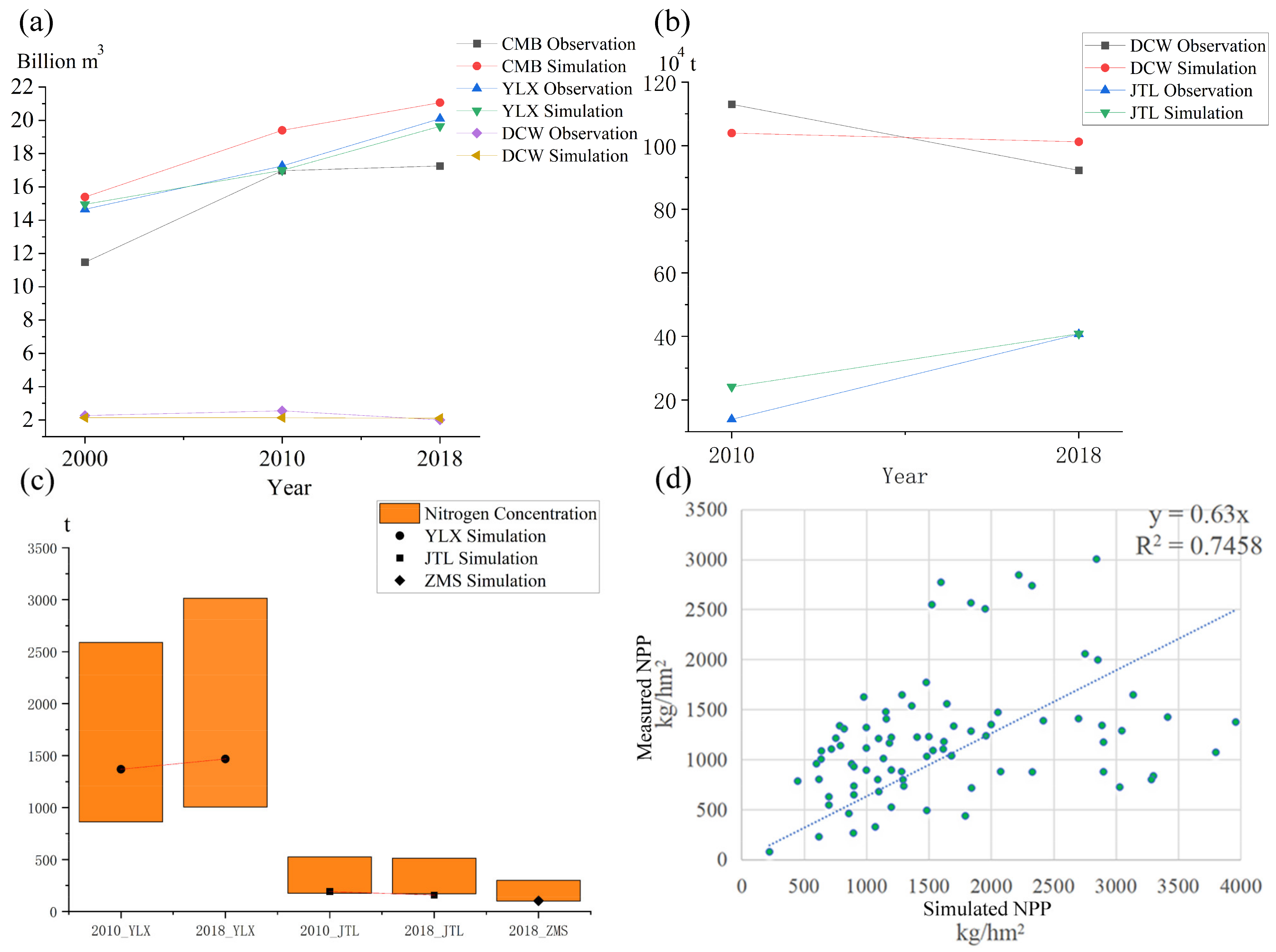
3.1. Verification of Model Simulation Results

Verification of model simulation showed the following: (1) Regarding water resource supply (Figure 3a), when the Zhang coefficients of the InVEST model in 2000, 2010, and 2018 were 2.5, 2.5, and 3.5, the overall accuracy of the model was 86.0%, 89.2%, and 90.2%, respectively. Further, the water yield simulation results showed good credibility, and the obtained results were realistic and accurate. (2) Regarding soil conservation (Figure 3b), the accuracy of the simulation results of soil conservation in 2010 and 2018 was 60.0% and 95.0%, and the overall accuracy was 77.5%, which proved that the InVEST model met the requirements for evaluating soil conservation services in the study area. (3) Regarding water purification (Figure 3c), during the study period, the nitrogen export results simulated by the nutrient delivery ratio module of the InVEST model were all within the concentration range of water quality observations at the hydrological station, proving that the model meets the research requirements. (4) Regarding climate regulation, the sampling yield of 2021 grassland quadrats was compared with the simulation results of the 2021 CASA model (Figure 3d), and the overall simulation accuracy of the CASA model was 63.6%. The R2 value of the linear fitting of grass yield and NPP was 0.7458, proving that the model-simulated NPP results and the actual sampling data have a good degree of fit. Therefore, the CASA model is applicable to the study of climate regulation services. These verification results provide confidence in the reliability and accuracy of the simulation outcomes obtained from the four models used in this study.

3.2. Changes in Ecosystem Areas

This study constructed a transfer matrix for the different ecosystems from 2000 to 2018 (Table 4) and analyzed the area served by each ecosystem (Table 5). In 2018, the dominant ecosystem type in the Qilian Mountains was grassland, covering 44.45% of the total land area. Desert, shrubland, and forest ecosystems accounted for 36.89%, 5.33%, and 3.31% of the total land area, respectively. The human settlement ecosystem was the smallest, accounting for only 0.2–0.3% of the total land area. Over the study period, significant changes in ecosystem areas were observed in the Qilian Mountains. Notably, there was a decrease in desert and glacier areas. The areas of grassland, forest, farmland, water, wetland, and human settlement ecosystems increased, while the area of the shrubland ecosystem remained relatively constant.
During the study period, desert ecosystems had the largest net transfer outflows, with a total transfer of 4099.35 km2, primarily to the grassland ecosystems (Table 5). Between 2000 and 2010, there was a significant transfer of the desert ecosystem to the grassland ecosystem, totaling 3858.96 km2. The glacier ecosystem experienced a net outflow of 215.84 km2, most of which transferred to the desert and grassland ecosystems, with limited transfers to the shrubland and wetland ecosystems. The grassland ecosystem showed the largest net transfer of 3568.51 km2 from the desert ecosystem. While the area of the grassland ecosystem increased significantly, a small part of the grassland ecosystem turned into human settlements, farmland, forest, and water ecosystems. The main source of the increase in the forest ecosystem was the transfer of the desert and grassland ecosystems, which was 68.92 km2 and 18.05 km2, respectively. The area of the water ecosystem increased from the desert, grassland, and wetland ecosystems, with an inflow of 85.21 km2, 55.27 km2, and 37.80 km2, respectively. Except for the glacier and water ecosystems, all other ecosystems in the Qilian Mountains underwent a transformation into human settlement ecosystems. Among them, the grassland ecosystem had the largest transformation area (56.26 km2). The grassland ecosystem was the main source of the increase in the area of the farmland ecosystem, with a transferred area of 229.78 km2. The area of the water ecosystem increased slightly, and 267 km2 of the desert ecosystem was transferred to it.

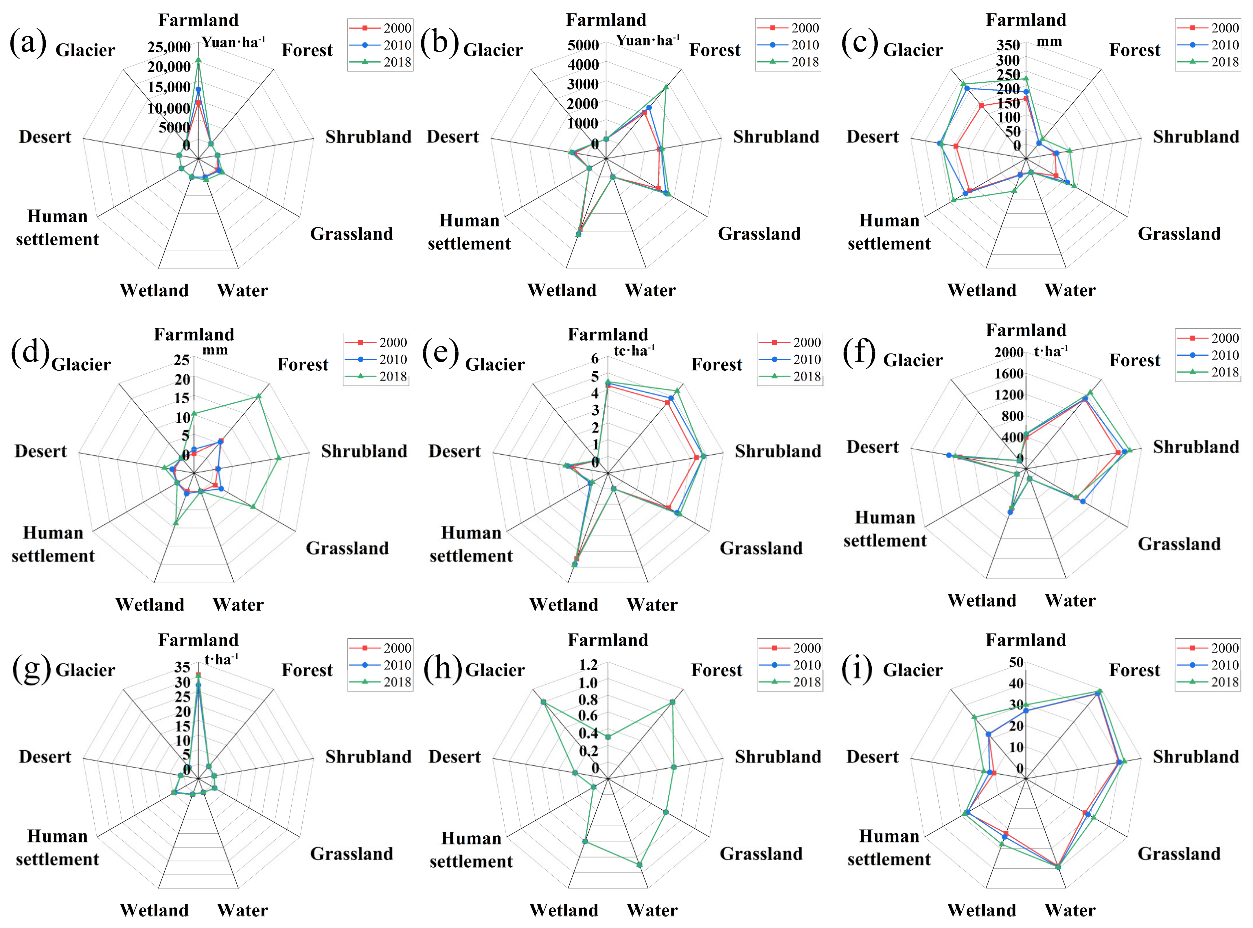
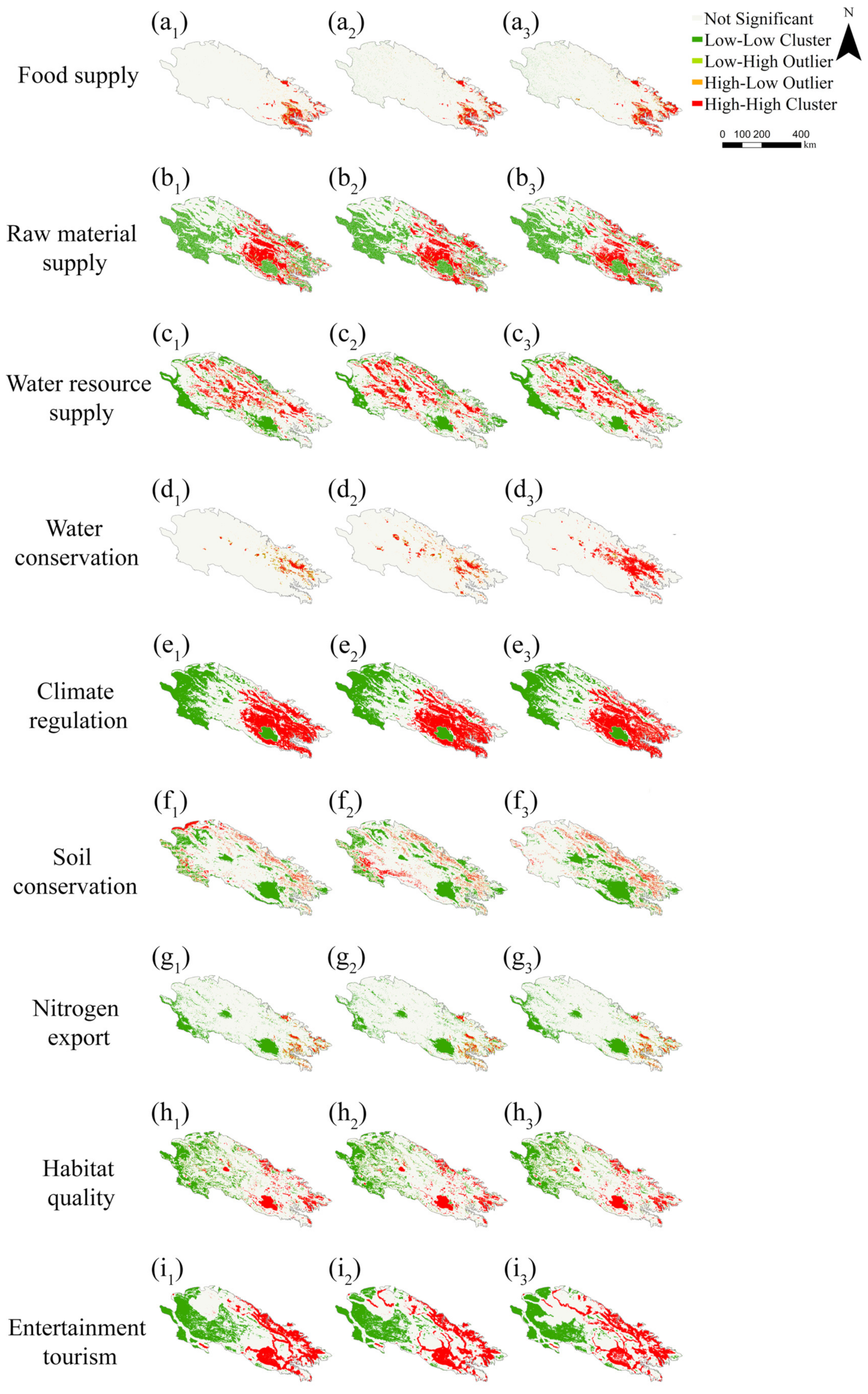
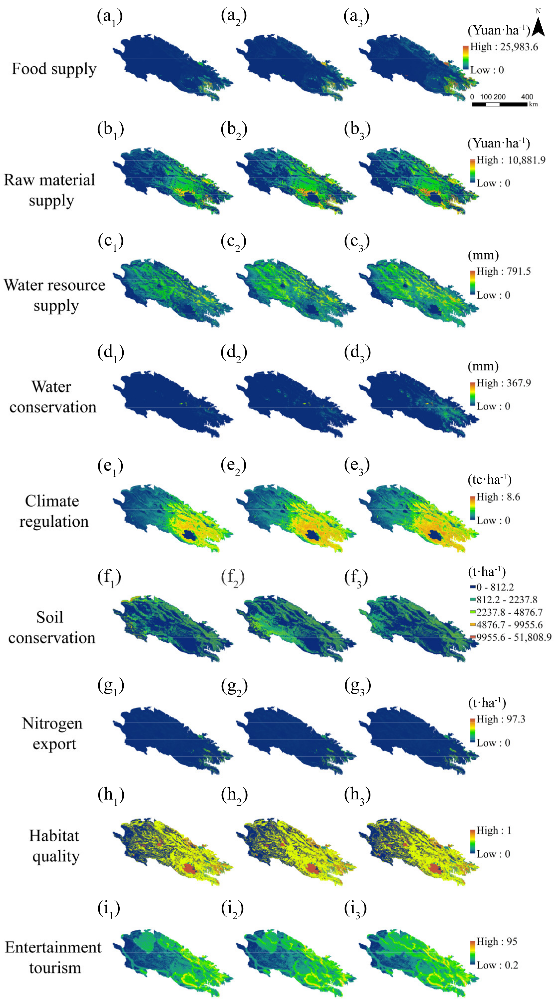
3.3. Identification of Ecosystem Services and Hotspots in the Qilian Mountains

During the study period, the Qilian Mountains exhibited clear increases in the food supply, raw material supply, water resource supply, water conservation, climate regulation, and entertainment tourism services (Table 6). Food supply and raw material supply in the area increased by 1038.83 and 448.21 Yuan·ha−1, respectively. Water resource supply and water conservation increased by 55.45 mm and 7.80 mm in 2018 compared to 2000. Climate regulation improved by 0.60 tc·ha−1, indicating an enhancement in the ecosystem’s capacity to regulate climate. Entertainment tourism increased to 26.76. Nitrogen export and habitat quality remained stable, and soil conservation showed a fluctuating growth trend, increasing by 40.01 t·ha−1 over the study period.
During the study period, various ecosystem services in the Qilian Mountains exhibited distinct characteristics (Figure 4).
During the study period, the farmland ecosystem had the largest food supply capacity, with a mean capacity of 20,396.62 yuan·ha−1 in 2018, followed by the grassland ecosystem, with a capacity of 2178.36 yuan·ha−1 (Figure 4a).
In 2018, the forest ecosystem had the strongest raw material supply capacity, with a mean annual raw material supply of 3773.70 yuan·ha−1, followed by the wetland ecosystem with 3178.51 yuan·ha−1, and the grassland ecosystem with 2707.44 yuan·ha−1 (Figure 4b). The raw material supply of the forest ecosystem increased significantly to 82.48% from 2000 to 2018. The increase in the raw material supply of the wetland and grassland ecosystems was 10.03% and 30.01%, respectively.
The mean annual water yield of the study area was 146.67 mm, of which the glacier ecosystem had the largest annual mean water yield of 244.29 mm·ha−1, and the desert ecosystem had the second largest annual mean water yield of 228.47 mm·ha−1 (Figure 4c). The mean water conservation capacity of the forest ecosystem was the highest at 20.71 mm·ha−1 in 2018 (Figure 4d).
The mean climate regulation service in 2018 was 3.05 tc·ha−1, an increase of 0.59 tc·ha−1 compared with that in 2000 (Figure 4e). The forest ecosystem had the largest annual mean climate regulation service (4.94 tc·ha−1).
The mean soil conservation capacity in the study area was 1026.04 t·ha−1, and the three ecosystems with the largest soil conservation capacities were the shrubland, forest, and desert ecosystems. Perennial mean soil conservation was 1668.93 t·ha−1, 1570.57 t·ha−1, and 1159.30 t·ha−1 in 2000, 2010, and 2018, respectively (Figure 4f).
During the study period, the glacier ecosystem had the lowest nitrogen export, and the farmland ecosystem had the largest nitrogen export. The mean nitrogen export in 2018 was 30.20 t·ha−1, and the nitrogen export capacity of each ecosystem remained unchanged (Figure 4g).
The habitat quality of glacial ecosystems was the highest in the study area, followed by forest ecosystems. The desert ecosystem was the natural ecological system with the lowest-quality habitat. During the period of the study, the mean habitat quality increased from 0.457 in 2000 to 0.466 in 2018 (Figure 4h).
Forest ecosystems had the highest entertainment tourism services, followed by shrubland and water ecosystems. During the study period, the entertainment tourism services of the glacier ecosystem improved significantly (Figure 4i).
These findings provide valuable insights into the diverse ecosystem services and their dynamics in the Qilian Mountains, highlighting the importance of different eco-systems in supporting various aspects of human well-being.
Table 7 shows that the global Moran I values of ES in the Qilian Mountains from 2000 to 2018 were all positive, and the p values were all less than 0.001, indicating that ES in the Qilian Mountains interacted with one another on the grid scale and showed the characteristics of aggregation distribution. Specifically, the value of the global Moran’s I index for food supply service was the largest, which indicated that food supply was the most concentrated in spatial distribution and had the strongest spatial aggregation. The global Moran’s I value of nitrogen export was the smallest, with the smallest spatial autocorrelation and the weakest spatial aggregation, showing the characteristics of agglomeration in a small range. During the study period, the global Moran’s I value of raw material supply, climate regulation, soil conservation, and habitat quality services increased gradually, indicating an increase in spatial aggregation and a progressively stronger spatial autocorrelation. The global Moran’s I value of food supply and nitrogen export gradually decreased, and the spatial autocorrelation gradually weakened.
To further determine the spatial distribution of each ES aggregation area and the trade-off and synergistic relations between different ES, local Moran’s I was employed, providing insights on the spatial distribution characteristics. Local Moran’s I divided the spatial relations into high–high, high–low, low–high, and low–low aggregation.
The spatial distribution of ES hotspots in the Qilian Mountains remained relatively stable throughout the study period, except for notable increases in hotspots for water conservation and entertainment tourism (Figure 5). The high-value regions of climate regulation were concentrated in the eastern Qilian Mountains. Furthermore, there was a significant spatial overlap of high-high aggregations between food supply, raw material supply, and entertainment tourism services, indicating a positive correlation among them (Figure 5(a1–a3,b1–b3,e1–e3,i1–i3)). In terms of water-related ES, the high-value areas for water resource supply and water conservation exhibited spatial aggregations in the eastern region of the study area, suggesting a cooperative relationship between these two services (Figure 5(c1–c3,d1–d3)). However, there were distinct spatial patterns observed. For instance, the Qinghai Lake basin showed a high–high aggregation area for habitat quality but a low aggregation area for water resource supply. In contrast, the western region displayed a low aggregation area for habitat quality, while the high-altitude mountainous areas in the west showed high-value areas for water resource supply, indicating a negative correlation in their spatial distribution (Figure 5(c1–c3,h1–h3)).
The application of Local Moran’s I analysis revealed the intricate spatial patterns and interrelationships between different ES in the Qilian Mountains. Understanding these spatial dynamics is crucial for informed decision-making and sustainable management of the region’s ecosystems.

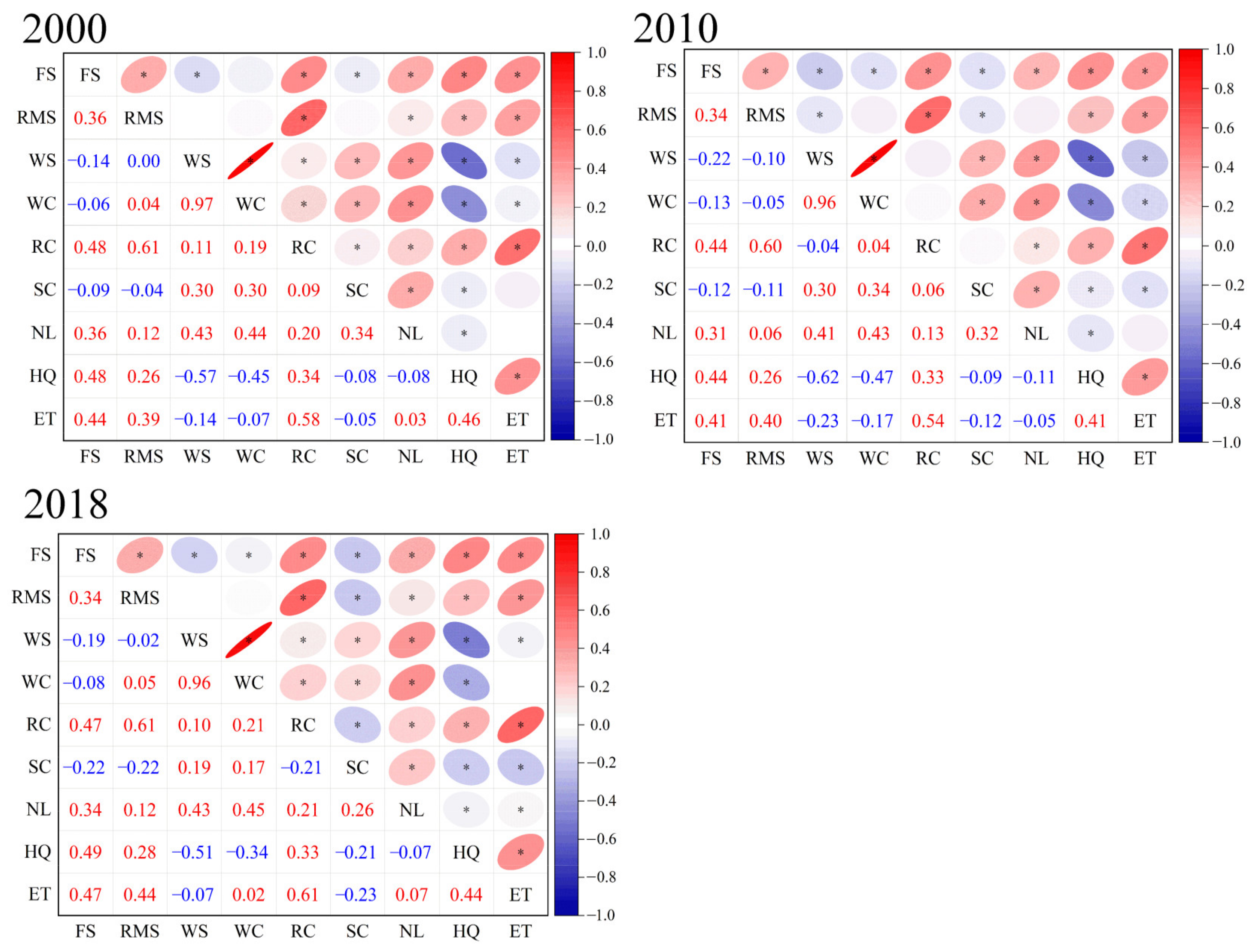
3.4. Trade-Offs and Synergies between ES

Spearman correlation analysis was conducted to assess the correlation among the nine ES in the Qilian Mountains (Figure 6). During the study period, the strongest synergy was observed between water resource supply and water conservation services, with a correlation coefficient of 0.97. Food supply, raw material supply, climate regulation, habitat quality, and entertainment tourism showed synergistic relationships with any two of these five services. In addition, soil conservation, water resource supply, and water conservation showed synergistic relationships with one another, and the correlation coefficient showed an obvious trend of an initial increase followed by a decrease during the study period.
Nitrogen export demonstrated a synergistic relationship with six services: food supply, raw material supply, water resource supply, water conservation, climate regulation, and soil conservation. Thus, there was a trade-off relationship between these six services and the water purification service. There was a synergistic relationship between the water purification service and habitat quality, and the correlation coefficient first increased and then decreased. Soil conservation had a trade-off relationship with food and raw material supply, and the correlation coefficient first increased and then decreased. The relationship between habitat quality and three services, namely water resource supply, water conservation, and soil conservation, is a trade-off relationship. Water resource supply had a trade-off relationship with food supply, habitat quality, and entertainment tourism, and the correlation coefficient between water resource supply and entertainment tourism first increased and then decreased.

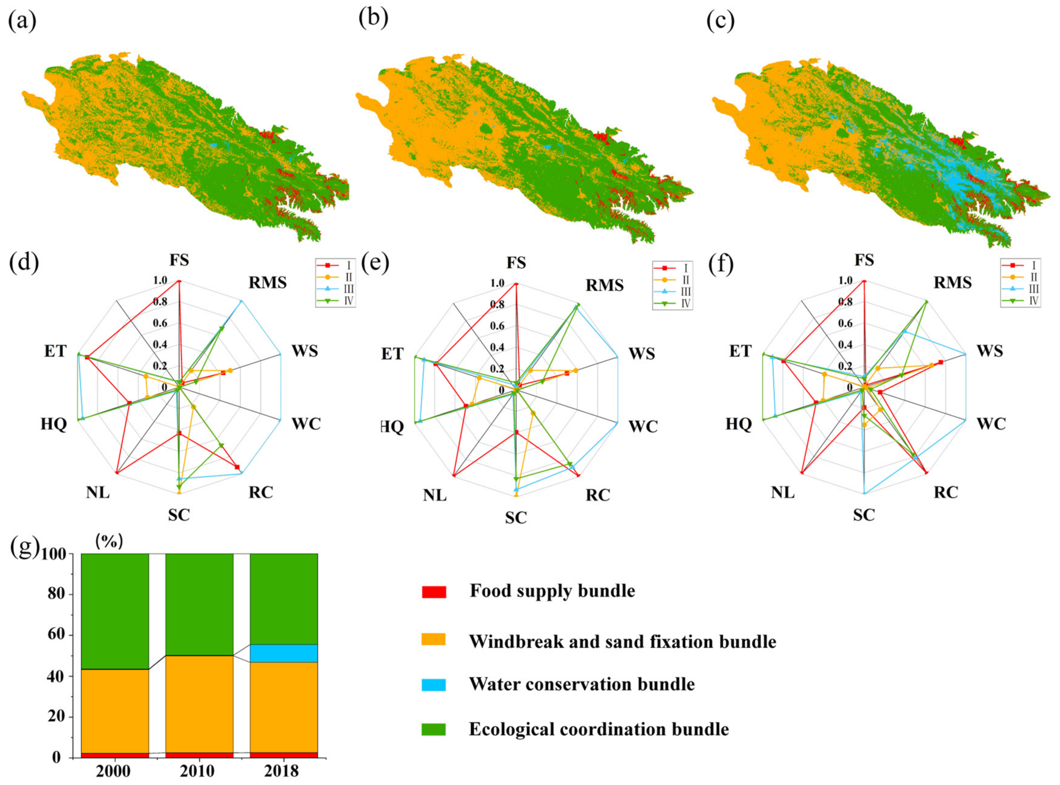
3.5. k-Means Clustering Analysis

By using k-means clustering analysis, four types of ecosystem service clusters were identified in the Qilian Mountains (Figure 7). The results showed that the same ESB has obvious aggregation relationships in space, and different bundles show significant differences. According to the characteristics of the ESB, they were named food supply, windbreak and sand fixation, water conservation, and ecological coordination bundles.
The food supply bundle was mainly located at the southeastern edge of the Qilian Mountains, and the ecosystem type was predominantly farmland (Figure 7a–c). During the study period, the area proportion of these ESB increased slightly, with an average proportion of approximately 2.5% (Figure 7g). In this service bundle, human activity was intense, agricultural production activity was frequent, and ecosystems were fragile. In addition, food supply, water purification, and climate regulation services were high, but raw material supply, habitat quality, and entertainment tourism services were relatively low (Figure 7d–f). With population growth in the Qilian Mountains, the demand for food supply services will increase, affecting the regional supply and demand structure. This may lead to the continuous expansion of the food production bundle, which would have a negative impact on the ecological balance of the surrounding areas.
The windbreak and sand fixation bundle were mainly distributed in the western Qilian Mountains and had a single ES function. The main vegetation types were desert and alpine steppe, and most glaciers in the Qilian Mountains were also distributed in this region (Figure 7a–c). During the study period, the area proportion of these ESB showed a trend of fluctuating increase, accounting for approximately 44.2% in 2018 (Figure 7g). These ESB had higher soil conservation and water resource supply services, but the food supply, water conservation, habitat quality, and entertainment tourism services were all lower than the mean level of the study area (Figure 7d–f). It is worth noting that although the vegetation coverage in the windbreak and sand fixation bundles is low, the actual wind erosion in the region is still far lower than the potential wind erosion, which is of great significance for weakening the wind erosion intensity, resisting wind sand, preventing desert expansion, and maintaining water and soil.
The water conservation bundle was mainly distributed in the middle of the Qilian Mountains and was characterized by strong water conservation ability (Figure 7a–c). In addition to the low food supply service, this ESB had an extremely high-water resource supply, water containment and soil conservation services, and relatively high raw material supply, water purification, climate regulation, habitat quality, and entertainment tourism services. This bundle was in good ecological condition, belonging to the ecological surplus area (Figure 7d–f). From 2000 to 2018, the area of the water conservation bundle increased significantly from 0.2% to 8.8% (Figure 7g). The increasing area was mainly concentrated in the eastern forest and grassland ecosystems, which had better water and thermal conditions, high vegetation coverage, and a good water conservation function.
The ecological coordination bundles were mainly concentrated in the eastern Qilian Mountains (Figure 7a–c). This bundle exhibited elevated levels of raw material supply, climate regulation, soil conservation, water purification, habitat quality, entertainment tourism services, and low food supply services, which were mainly grassland, forest, and shrubland ecosystems (Figure 7d–f). During the study period, this service cluster area showed a decreasing trend, accounting for approximately 44.5% in 2018 (Figure 7g).

4. Discussion

4.1. Temporal and Spatial Evolution of ES

The ecosystem processes in the Qilian Mountains, including the water and carbon cycles, vegetation growth, and material and energy exchange, involve complex interactions and mutual influences. The distribution structure of ES exhibits heterogeneity due to unevenly distributed factors such as geology, topography, and hydrology, as well as social factors such as road networks, population distribution, and economic development levels [74].
Atmospheric water vapor and surface precipitation in the Qilian Mountains are affected by westerly wind belts, southerly monsoons, and the East Asian monsoon [81]. In recent decades, under the influence of global warming, the Qilian Mountains have shown a trend of warming and humidification. The characteristics of warming and humidification were obvious, and rainfall increased significantly, showing a higher spatial distribution in the southeast and lower spatial distribution in the northwest [82,83]. As a result, vegetation coverage in the eastern region was significantly higher than that in the western region. In the past 20 years, the glaciers in the Qilian Mountains have melted, and the snow line has moved up, which has a significant impact on the runoff out of the mountain pass [84]. In addition, the actual evaporation in the alpine region is small, the soil water holding capacity is weak, and the local runoff is easily formed, which leads to a strong water-producing capacity. Water conservation capacity and water resource supply were closely related in the study area, showing an obvious synergistic relationship. In the western Qilian Mountains, vegetation is sparse, and the ability to intercept precipitation is poor, resulting in a low water conservation capacity compared to areas with high vegetation coverage. Forests have the strongest water conservation capacity, which mainly includes the canopy and litter interception of precipitation and soil water storage to keep water in the soil for a long time [85]. On the one hand, farmland ecosystems are the most important source of food supply; on the other hand, farmland ecosystems have the largest nitrogen export but have a poor water purification ability, which is also the main factor leading to water eutrophication.
Climate regulation services in the Qilian Mountains increased annually during the study period, which is in accordance with the results of previous studies [86,87], and there is a good coupling relationship between the size of climate regulation services and the spatial variation trend of vegetation coverage [88]. Areas with high soil conservation value are predominantly found in the forest, shrubland, and grassland ecosystems with high vegetation cover in the eastern Qilian Mountains, as well as fragile desert and alpine grasslands in the west, which require priority protection measures. The grassland ecosystem accounted for approximately 44% of the total study area and had the highest amount of soil conservation of all ecosystem areas. Although the northwest region had less rainfall, dominant wind erosion, and low vegetation coverage, the desert vegetation in this region had a considerable amount of soil conservation.
During the study period, habitat quality in the Qilian Mountains was relatively high and stable, although a slightly increasing trend was observed. Owing to climate change, glacier retreat [84], urban expansion, and human activities, ecological degradation has occurred in some areas of the Qilian Mountains. Therefore, managing and developing land resources more scientifically and sensibly, maintaining biodiversity, and promoting sustainable development are still critical issues that need continuous attention from the academic community. Simultaneously, it is of great significance to protect the sparse grassland ecosystem in the high-altitude area of the Qilian Mountains through the further prohibition of grazing by either closing or implementing seasonal grazing of grasslands with different coverage, which will help maintain the stability of the ecosystem.
The continuous improvement of transportation facilities further improves the accessibility of tourism and expands the tourism attraction of the Qilian Mountains and surrounding areas, especially the entertainment tourism service of glaciers. Given the uniqueness and significance of the region’s glaciers, they have become hotspots for scientific research and climate change investigation. Glacier resources are scarce and possess high tourism value [89]. Thus, this ecosystem plays a vital role in promoting local economic development, providing employment opportunities, increasing the income of residents, and maximizing social benefits. It is crucial to protect, plan, and develop glacier resources based on the principles of protection priority and sustainable utilization.

4.2. Trade-Offs and Synergies of ES

The Qilian Mountains exhibit a strong synergistic relationship between water conservation and water resource supply, which is in line with previous research [90]. Precipitation and evapotranspiration jointly affect the spatial distribution of regional water production, and the vegetation coverage and soil conservation of precipitation determine the capacity for water conservation. Therefore, regions with sufficient precipitation and high vegetation coverage are conducive to regional water production and conservation, leading to a synergistic relation between water resource supply and conservation. The positive correlation between water resource supply and soil conservation aligns with previous studies [91,92]. This is mainly because vegetation coverage is directly affected by the supply of water resources. In areas with good hydrothermal conditions, increased precipitation will promote the growth and development of plants. The subsequent increase in vegetation coverage will improve resistance to soil erosion and reduce water and wind erosion, which is conducive to soil conservation [65]. Water resource supply and habitat quality had a trade-off relationship, which was due to the apparent vegetation recovery in the Qilian Mountains in recent years. The areas of the forest and grassland ecosystems increased significantly, and habitat quality improved. However, with an increase in vegetation coverage, evapotranspiration increased, surface runoff decreased, and water resource supply decreased. This is consistent with previous research findings [64].
There was a strong positive correlation between food supply and nitrogen export. Therefore, compared to the other ecosystems, the farmland ecosystem had the highest food supply service and nitrogen export capacity and the lowest water purification capacity. The reason for this is that the use of chemical fertilizers increases with an increase in the regional food supply service, which leads to an increase in nitrogen export [93]. Hence, a synergistic relationship exists between food supply and nitrogen export, while a trade-off relationship is observed between food supply and water purification services. Additionally, a weak trade-off relationship exists among soil conservation, food supply, and raw material supply, consistent with previous findings [28,94,95]. The amount of chemical fertilizer that is applied is a crucial factor in determining the trade-off relationship between food supply and soil conservation [96].
There is a strong trade-off relationship between water resources and food supply [93,97]. The main reason for this is that agricultural production consumes a significant amount of water resources, which decreases the amount of surface runoff. This reflects the inherent conflict between food production and water resource use and environmental protection in a specific region [21,26].

4.3. k-Means Clustering and Suggestions on Zoning Management

There is clear spatial heterogeneity in ES and its trade-offs [98]. Ecosystem management aims to enhance one or more ES. According to the trade-offs and synergies between ES, ecological protection and management measures are adopted according to local conditions. This approach is crucial for improving key regional ES, enhancing overall ecological benefits, and providing decision-making support for regional development and ecological construction [25]. The analysis of trade-offs and synergies between ES is the basis for the effective management of the ecosystem of the Qilian Mountains. The division of ES is an effective aid in the formulation of regional management policies [99].
ESB form different spatial relationships with the comprehensive action of the society-ecological environment, and this relationship changes over time [36]. From the perspective of the evolution of ESB, the reason for this change is a combination of climate change and human activities [25]. Recent decades have witnessed a significant increase in precipitation and a warming trend in the Qilian Mountains [82,83]. Simultaneously, with the increase in regional population, the demand for food supply services will increase, and land with good water, soil, light, and heat conditions will be reclaimed for use as farmlands, which will lead to trade-offs between different ES in some areas [25]. The food supply bundle of the Qilian Mountains was dominated by the farmland ecosystem, and there is a spatial trade-off between the food supply and water resource supply services, which is associated with the large number of water resources required for food production [97]. The windbreak and sand fixation bundle were located northwest of the Qilian Mountains. Owing to the poor hydrothermal conditions in this area, a landscape with low vegetation coverage, desert, and sparse grassland was formed. In addition to soil conservation, all ES in this area were low. The ecological functions of windbreak and sand fixation guarantee ecological security in the fragile desert area of western China. The area covered by the water conservation bundle in the central region increases annually. Compared with other bundles, this bundle shows a strong water conservation ability, which is related to high vegetation coverage and the strong ability of this region to intercept, infiltrate, and store precipitation. The variety of ES in the ecological coordination bundle was greater than the average level of the study area, which was largely related to the wide distribution of grassland ecosystems in the region. Pasture, as the main food source of livestock, contributes to animal husbandry development. Grasslands also play a significant role in carbon dioxide absorption through photosynthesis, contributing to climate regulation. Hence, this bundle shows high supply and regulation services.
The purpose of ecosystem management is to enhance one or several ES and divide the study area into different ESB according to the spatial distribution characteristics of the ecosystem. The goal of this is to clarify the objectives of regional management and take protection measures according to local conditions, which will improve the value of key ES in a region and enhance the overall benefits of regional ES. Thus, it is important to maintain the sustainable development of ecosystems.
Based on our results from the four types of ESB, the following suggestions are made: (1) Food supply bundle: strict adherence to ecological protection guidelines and safeguarding food security are imperative. Enforcing laws and regulations on land use, prohibiting unauthorized cultivation, strengthening water and soil conservation, and improving ecosystem stability are recommended. (2) Windbreak and sand fixation bundle: in the future, we should optimize the scope of the red line of ecological protection, focus on protection, reduce the intensity of human activities, adopt ecological improvement, increase the vegetation coverage under appropriate natural conditions, strengthen the ecological control mode of ecological restoration, set up ecological restoration demonstration areas to improve the quality of the eco-environment and service functions, and give full effect to the role of ecological security barriers in western China. (3) Water conservation bundle: all activities that disrupt ecological balance and cause water pollution should be prohibited. The utilization of water resources should be sensibly controlled, soil and water conservation forests should be widely planted, closed management should be adopted, and grazing and other production activities should be strictly prohibited to reduce the interference of human activities as much as possible and reduce ecological risks. (4) Adhering to ecological protection principles as a priority and allowing economic development. We will continue implementing the policy of herbage and livestock balance, strengthening ecological protection and restoration, and improving regional ecological functions and service capacity.

4.4. Strengths, Limitations, and Future Research

One strength of the study is its use of correlation coefficients to analyze trade-off and synergy relationships among different ecosystem services (ES). Although correlation coefficients provide insights into these relationships, they may not fully capture the underlying mechanisms driving trade-offs and synergies [100,101]. Future research should explore these mechanisms to gain a deeper understanding of the causes and dynamics of trade-offs and synergy relationships among ES.
Another limitation of the study is its focus on analyzing trade-offs and spatial bundles of ES without considering the specific driving factors that influence the spatial and temporal distribution of different ES. It is important to investigate the specific factors that contribute to these patterns, as they can provide valuable insights for effective ecosystem management. Future research should aim to identify and analyze the driving factors that influence ES distribution, considering both natural and human-induced factors.
The use of k-means clustering in this study is a valuable approach to ecological partitioning. It overcomes some of the subjectivity associated with previous methods. However, it is important to note that the algorithm itself is a tool, and a more scientific and persuasive ecological partitioning can be achieved by combining the algorithm with expert suggestions from relevant fields. Future research should explore ways to integrate objective algorithms with expert knowledge to enhance the accuracy and robustness of ecological partitioning.
Future research should also consider the scale effect of trade-offs and synergy relationships among ES. Understanding how these relationships vary at different scales can provide valuable insights for ecosystem management and decision-making. Additionally, exploring the threshold of driving factors can help identify critical points at which trade-offs and synergies become more pronounced or shift. This knowledge can inform targeted interventions and management strategies.
In summary, future research should delve into the underlying mechanisms driving trade-offs and synergies among ES, investigate the specific driving factors influencing ES distribution, explore the integration of objective algorithms with expert suggestions, consider the scale effect of trade-offs and synergies, and identify thresholds in driving factors. By addressing these aspects, a more comprehensive understanding of ES dynamics and effective ecosystem management strategies can be achieved.

5. Conclusions

The spatial and temporal patterns and changes in the characteristics of different ES exhibit distinct patterns and changes influenced by global climate change and human activities. Regarding spatial distribution, the high-value area of food supply services was mainly concentrated in the farmland ecosystem in the southeast, which was the low-value area of water purification services. The high-value areas for water resource supply services were mainly located in the high-altitude mountainous areas. Forest ecosystems were the high-value areas for water conservation, climate regulation, and habitat quality services. The high-value areas for raw material supply services were mainly concentrated in the eastern grassland and forest ecosystems. The high-value areas for soil conservation services were concentrated in the western and eastern parts of the Qilian Mountains, where the former was a high-value area for preventing wind erosion, with the desert as the main ecosystem type, and the latter was a high-value area for preventing hydraulic erosion, with forest and shrubland as the main ecosystems. The high-value areas for entertainment tourism services were mainly distributed around Qinghai Lake and in the eastern forest and shrubland ecosystems. During the study period, in addition to habitat quality and water purification, which remained unchanged, and soil conservation, which showed a fluctuating growth trend, six ES (food supply, raw material supply, water resource supply, water conservation, climate regulation, and entertainment tourism) showed a significant increase, and the overall ecology of the Qilian Mountains continued to improve.
Trade-offs and synergistic relationships among ES affected the spatial distribution of ESB. The food supply bundle was dominated by farmland ecosystems, which exhibited high food supply, high climate regulation, and low water purification services, and the division of this bundle was related to the synergistic relationship between food supply and climate regulation services and the trade-off relationship between food supply and water purification services. The windbreak and sand fixation bundle were dominated by grassland ecosystems, which showed high soil conservation, higher water resource supply, and low habitat quality services; the classification of this bundle was related to the synergistic relationship between soil conservation and water resource supply and habitat quality had a trade-off relationship with soil conservation and water resource supply. The water conservation bundle was dominated by forest and grassland ecosystems, which exhibited high water resource supply, water conservation, and soil conservation services, and the division of this bundle was related to the synergistic relationship among water resource supply, water conservation, and soil conservation. The ecological coordinated bundle was dominated by grassland, forest, and shrubland ecosystems, which showed high raw material supply, climate regulation, habitat quality, and entertainment tourism services, and the division of this bundle was related to the synergistic relationship among raw material supply, climate regulation, habitat quality, and entertainment tourism services. Further research should focus on the drivers and thresholds of ES to address the impacts of future climate change on ecosystem management.

Author Contributions

Conceptualization, H.C., N.W., and Y.W. (Yipeng Wang); methodology, Y.W. (Yipeng Wang); software, Y.W. (Yipeng Wang); validation, Y.W. (Yipeng Wang); formal analysis, Y.W. (Yipeng Wang); investigation, Y.W. (Yipeng Wang), H.C., N.W., C.H., K.Z., B.Q., Y.W. (Yuanyuan Wang), and P.W.; resources, H.C. and N.W.; data curation, Y.W. (Yipeng Wang); writing—original draft preparation, Y.W. (Yipeng Wang); writing—review and editing, Y.W. (Yipeng Wang), H.C., and N.W.; visualization, Y.W. (Yipeng Wang); supervision, H.C. and N.W.; project administration, N.W.; funding acquisition, H.C. and N.W. All authors have read and agreed to the published version of the manuscript.

Funding

This research was funded by the National Key Research and Development Program of China (Grant No. 2019YFC0507402) and Gansu Province Science and Technology Project (Grant No. 22JR5RA161).

Data Availability Statement

The data presented in this study are available on request from the corresponding author.

Conflicts of Interest

The authors declare no conflict of interest. The funders had no role in the design of the study; in the collection, analyses, or interpretation of data; in the writing of the manuscript, or in the decision to publish the results.

Appendix A

Appendix A.1. Changes in Spatial and Temporal Patterns of Ecosystem Services in the Qilian Mountains

The spatial and temporal distributions of different ES in the Qilian Mountains exhibit clear heterogeneity, as depicted in Figure A1. Throughout the study period, the spatial distribution pattern of food supply services remained consistent. The high-value areas were primarily concentrated in the farmland ecosystem around the southeastern region, while the low-value areas were mainly focused on the desert ecosystem in the northwestern region (Figure A1(a1–a3)).
Similarly, the spatial pattern of the water purification service remained unchanged. Regions with limited water purification ability were predominantly observed in the southeastern farmland ecosystem, where the output of nitrogen was extremely high. Conversely, areas with high water purification capability were mainly concentrated in the eastern forest ecosystem (Figure A1(g1–g3)).
Regarding raw material supply, the high-value areas were distributed in the grassland ecosystem surrounding Qinghai Lake and the eastern forest ecosystem. In contrast, the alpine meadow area at high altitudes represented the low-value area (Figure A1(b1–b3)).
The spatial distribution of the water resource supply service in the Qilian Mountains exhibited variations. High-value areas were primarily concentrated in high-altitude mountainous areas, characterized by abundant precipitation, sparse vegetation, limited soil infiltration capacity, and easy surface runoff formation. On the other hand, the low-value areas were mainly located in the northwestern region, characterized by low precipitation, strong evaporation, and mainly desert ecosystems (Figure A1(c1–c3)).
Regarding the water conservation service, the high-value areas of the water conservation service were mainly concentrated in forest and grassland ecosystems in the eastern region. Throughout the study period, there was a significant increase in the high-value water conservation areas, primarily expanding in the eastern forest ecosystem and the high-coverage grassland with higher vegetation coverage and favorable water and heat conditions (Figure A1(d1–d3)).
The spatial distribution of the climate regulation service demonstrated distinct characteristics, with low values in the western region and high values in the eastern region. The high-value regions were concentrated in the Qinghai Lake basin and the eastern forest ecosystem, which benefit from favorable hydrothermal conditions promoting vegetation growth (Figure A1(e1–e3)).
The soil conservation service in the Qilian Mountains exhibited distinct spatial patterns. The high-value regions were concentrated in the western and eastern parts of the Qilian Mountains, while low-value regions were mainly found in glaciers and surrounding desert ecosystems (Figure A1(f1–f3)). The western region, characterized by high sunshine intensity, a large diurnal temperature range, little precipitation, strong evaporation, and wind erosion, played a dominant role. As a result, it was identified as a high-value area for preventing wind erosion in the desert ecosystem, contributing to significant soil conservation in that area. In contrast, the eastern region received more precipitation, with hydraulic erosion being the dominant erosional process. The forest and shrubland ecosystems in the eastern region were identified as high-value areas for soil conservation.
Habitat quality showed notable variations between the eastern and western regions, with the eastern region exhibiting significantly higher habitat quality compared to the western region (Figure A1(h1–h3)). However, it is worth noting that the continuous melting of glaciers has led to the transformation of previously glacier-covered areas into bare lands without vegetation cover, leading to a slight reduction in the quality of mountain habitats in some areas.
The areas with high values of the entertainment tourism service were mainly distributed around Qinghai Lake and the regions characterized by concentrated forest and shrubland ecosystems in the eastern part of the Qilian Mountain. These areas possess a picturesque ecological environment and convenient transportation, making them suitable for tourism activities (Figure A1(i1–i3)).
Figure A1. Spatial distribution of ES in the Qilian Mountains from 2000 to 2018: (a1i3) represents food supply, raw material supply, water resource supply, water conservation, climate regulation, soil conservation, nitrogen export, habitat quality, and entertainment tourism services, respectively; the subscript (1–3) represents the years 2000, 2010, and 2018, respectively.
Remotesensing 15 02950 g0a1

Appendix A.2. InVEST Models and Parameterization

Appendix A.2.1. Water Yield Model

The water yield module is based on the Budyko water-heat coupling equilibrium hypothesis [53], and the calculation formula is as follows:
Y x = 1 A E T x P x × P x
A E T x P x = 1 + P E T x P x 1 + P E T x P x ω 1 ω
P E T x = K c l x · E T 0 x
ω x = Z A W C x P x + 1.25
E T 0 = 0.408 Δ R n G + γ 900 T + 273 u 2 e s e a Δ + γ 1 + 0.34 u 2
A W C x = M i n R e s t l a y e r d e p t h , R o o t d e p t h · P A W C
where A E T x represents the annual actual evapotranspiration of the grid cells (mm); P x represents the annual precipitation of grid cells (mm); P E T x represents potential evapotranspiration; ω x represents the non-physical parameters of natural climate–soil properties; K c l x represents the evapotranspiration coefficient of plants (vegetation) for specific land use types in the grid; the minimum value of ω x is 1.25 [102]; and A W C x is the effective water content of the soil (mm), which is determined by the soil texture and effective depth. Z is an empirical constant that represents the regional precipitation distribution and other hydrogeological characteristics. E T 0 x represents the grid’s crop reference evapotranspiration; R n is net radiation (MJ/(m2·d)); G is soil heat flux (MJ/(m2·d)); γ is a constant on the wet and dry scale; T is the average daily temperature (°C); u 2 is 2 m wind speed (m/s); e s and e a are saturated and actual vapor pressure (kPa), respectively; δ is the slope of the saturated vapor pressure curve (kPa/°C); and PAWC is the available water content of plants. The calculation formula for PAWC is as follows [90]:
P A W C = 54.509 0.132 S A N 0.003 S A N 2 0.055 S I L 0.006 S I L 2 0.738 C L A + 0.007 C L A 2 2.668 C + 0.501 C 2
where SAN is the sand content (%), SIL is the silt content (%), CLA is the clay content (%), and C is the soil organic carbon content (%). The specific parameters of the water production model adopted in this study are listed in Table A1 [52,103].
Table A1. Parameters of water production model.
Land Use TypesKcRoot_Depth
Farmland0.6700
Forest17000
Shrubland0.854570
Grassland0.652000
Water11000
Wetland0.86300
Human settlement0.3500
Desert0.210
Glacier0.510
Kc, evapotranspiration coefficient.

Appendix A.2.2. Extension Model for Water Conservation

This study used the water balance equation to calculate the amount of water conservation. The computation formula is as follows [54,55,56]:
T Q = i = 1 n P i R i E T i · A i
where P i is the precipitation of the class i ecosystem (mm), R i is the surface runoff of the class i ecosystem (mm), E T i is the evapotranspiration of the class i ecosystem (mm), A i is the area of the class i ecosystem, and n is the number of ecosystem types in the study area.
The InVEST water production model calculates the water resource supply of each grid cell, i.e., the amount of water, by subtracting the actual evapotranspiration from the precipitation of each grid cell. Based on the water balance equation, the formula for calculating water conservation is as follows:
T Q = Y x R u n o f f i j
where R u n o f f i j (mm/a) is the surface runoff of pixel i in a class j ecosystem. Surface runoff was calculated according to the runoff coefficient and rainfall. The runoff coefficient is the ratio of rainfall to runoff volume. Influenced by several factors, the larger the runoff coefficient, the less easily rainfall is absorbed by soil [104]. By referring to the domestic literature on the precipitation and surface runoff of runoff districts in different ecosystems [56,105,106,107,108], combined with the climatic characteristics of the study area, vegetation coverage of different ecosystems, colony species, and other factors, the runoff coefficient was assigned, and the results are shown in Table A2.
Table A2. Reference values of surface runoff coefficients for each ecosystem type.
Ecosystem TypeRunoff Coefficient (%)
Farmland49
Forest3.52
Shrubland19.2
Grassland36
Water100
Wetland20
Human settlement80
Desert79
Glacier85

Appendix A.2.3. Sediment Delivery Ratio Module

In this study, the soil conservation module of the InVEST model was used to calculate soil conservation in the water erosion area. Based on the soil loss equation (RUSLE), this module can evaluate the soil conservation function more intuitively and rationally [109]. The calculation formula is as follows:
S C = R × K × L S × 1 C × P
where SC represents soil conservation (t·ha−1·a−1); R is rainfall erosivity; K is the amount of soil loss per unit area caused by unit rainfall erodibility (t·h·MJ−1·mm−1), which represents the erodibility of soil affected by soil texture, organic matter content, soil structure, permeability, and other factors, and reflects the anti-erosion ability of soil. LS is the slope length and slope factor, C is the vegetation cover factor, and P is the soil and water conservation factor. The calculation formula of soil erodibility factor K is as follows [110]:
K = 0.1317 0.2 + 0.3 e x p 0.0265 S A N 1 S I L 100 × S I L C L A + S I L 0.3   × 1 0.25 C C + e x p 3.72 2.95 C × 1 0.7 S N S N + e x p 22.9 S N 5.51
where SAN is the sand content (%), SIL is the silt content (%), CLA is the clay content (%), C is the soil organic carbon content (%), and SN = 1 − SAN/100. The mean annual rainfall was used to estimate the erosive force (R). The formula is as follows [111]:
R = α P β
where P is the average annual precipitation (mm), and R is the average annual rainfall erosivity (MJ·mm·ha−1·h−1·a−1). In this study, α and β are model parameters, which are 0.0668 and 1.6266, respectively [112].
According to relevant research results [52,113,114], the values of the vegetation cover factor (C) and soil and water conservation factor (P) were assigned based on the situation in the Qilian Mountains. The results are shown in Table A3 below.
Table A3. Vegetation cover factor (C) and soil and water conservation factor (P).
Land Use TypesUsle_cUsle_p
Farmland0.50.4
Forest0.0030.2
Shrubland0.010.2
Grassland0.020.25
Water0.0010.001
Wetland0.010.2
Human settlement0.0010.001
Desert0.250.01
Glacier10.001
The causes and erosion process of wind erosion are complex, and the parameters of most models are difficult to obtain. In addition, the models themselves have limitations. In this study, the drainage basin wind erosion model established by Dong et al. (1998) [57] was adopted, and the model formula was as follows:
t   x   y 3.9 1.0413 + 0.0441 θ + 0.0021 θ 2 0.0001 θ 3 V 2 8.2 × 10 5 V C R S D R 2 H 8 d 2 F , x , y , t d x   d y   d t
where θ is the slope (°), V is the wind speed (m/s), VCR is the vegetation coverage (%), and SDR is the damage rate of the artificial surface structure (%) that is obtained by referring to the hypothesis of the equation in the wind tunnel simulation, H is the relative humidity of air (%), d is the average particle size of soil particles (mm), F is the soil hardness (N/cm2), x and y represent the distance from the reference point, and t represents time (s). The formula for calculating the vegetation coverage is as follows:
V C R = N D V I N D V I s o i l N D V I v e g N D V I s o i l
The NDVI probability distribution values of 95% and 5% were used to determine the threshold NDVI values representing pixels completely covered by vegetation and the areas covered by bare soil or no vegetation, respectively. Soil wind erosion is a form of soil erosion that occurs without considering vegetation coverage. The vegetation’s contribution to soil conservation under wind erosion can be calculated as the difference between the potential soil wind erosion and the actual soil erosion, taking into account the protective effect of vegetation.

Appendix A.2.4. Nutrient Delivery Ratio (NDR) Module

The principle of the NDR module of the InVEST model is to calculate the long-term steady-state flow of nitrogen in the entire watershed based on the ability of different ecosystem types to transfer nitrogen into runoff and to reflect the water quality in the watershed according to the content of nitrogen in the water body. The higher the nitrogen content, the more serious the water pollution or eutrophication in the basin and the weaker the water purification capacity of the ecosystem in the basin. The nitrogen output of each grid was calculated based on the product of the nutrient load and NDR. The calculation formula is as follows:
x e x p i = l o a d s u r f , i · N D R s u r f , i + l o a d s u b s u r f , i · N D R s u b s u r f , i
x e x p t o t = i x e x p i
The nitrogen content of each grid was correlated with the nutrient load. Nutrient loads for each land use type are empirical coefficients based on nutrient output measurements [115].
m o d i f i e l d . l o a d i = l o a d i · R P I i
R P I i = R P i R P a v
l o a d s u r f , i = 1 p r o p o r t i o n s u b s u r f a c e i · m o d i f i e l d . l o a d n i
l o a d s u b s u r f , i = p r o p o r t i o n s u b s u r f a c e i · m o d i f i e d . l o a d n i
where R P I i is the runoff potential index of grid i ; R P i is the nutrient runoff proxy for runoff on pixel i ; R P a v is the average runoff potential over the entire area; p r o p o r t i o n _ s u b s u r f a c e i is the ratio parameter between the two nutrient sources; and N D R s u r f , i and N D R s u b s u r f , i are the nutrient transport ratios of the surface and subsurface, respectively.

Surface NDR

Surface N D R is the product of a delivery factor, representing the ability of downstream pixels to transport nutrients without retention, and a topographic index that represents the position on the landscape. For a pixel i :
N D R i = N D R 0 , i 1 + e x p I C 0 + I C i k 1
where I C 0 and k are calibration parameters, I C i is a topographic index, and N D R 0 , i is the proportion of nutrients that are not retained by the downstream pixels (irrespective of the position of the pixel on the landscape). Below, we provide details of the computation of each factor.
N D R 0 , i = 1 e f f i
e f f i = { e f f L U L C i · 1 S i i f   d o w n i   i s   a   s t r e a m   p i x e l e f f d o w n i · s i + e f f L U L C i · 1 S i i f   e f f L U L C i > e f f d o w n i e f f d o w n i o t h e r w i s e
where e f f d o w n i is the effective downstream retention on the pixel directly downstream from i , e f f L U L C i is the maximum retention efficiency that Land use types i can reach, and S i is the step factor defined as:
S i = exp 5 l i d o w n l L U L C i
where l i d o w n is the length of the flow path from pixel i to its downstream neighbor. This is the Euclidean distance between the centroids of two pixels. l L U L C i is the LULC retention length of the land cover type on pixel i .
I C = log 10 D u p D d n
D u p = S ¯ A
D d n = i d i S i
where I C is the connectivity index, S ¯ is the average slope gradient of the upslope contributing area (m/m), A is the upslope contributing area (m2), d i is the length of the flow path along pixel i according to the steepest downslope direction (m), and S i   is the slope gradient of pixel i .

Subsurface NDR

The expression for the subsurface NDR is a simple exponential decay with distance to stream, plateauing at the value corresponding to the user-defined maximum subsurface nutrient retention:
N D R s u b s , i = 1 e f f s u b s 1 e 5 l i l s u b s
where e f f s u b s is the maximum nutrient retention efficiency that can be reached through the subsurface flow, l i is the distance from the pixel to the stream, and l s u b s is the subsurface flow retention length.
Based on field investigations, background data collected in the study area, and relevant local and international research [52,116,117,118,119], we built an NDR model parameter table, as shown in Table A4.
Table A4. NDR model parameters.
Land-Use TypeLoad_nEff_n
Farmland67.20.15
Forest17.40.7
Shrubland20.80.6
Grassland11.50.45
Water0.0010.05
Wetland3.90.72
Human settlement100.05
Desert3.70.3
Glacier0.0010.05

Appendix A.2.5. Habitat Quality Module

Habitat quality simulated by the habitat quality module of the InVEST model can accurately reflect the status quo of habitat services [58]. The habitat quality index reflects the overall status of regional biodiversity. Roads, building land, farmland, and bare land are stress factors that threaten biodiversity. The calculation formula is as follows [120]:
Q x j = H j 1 D x j z D x j z + k z
D x j = r = 1 r y = 1 y ω r r = 1 R ω r r y i r x y β x S j r
i r x y = e x p 2.99 d r m a x d x y
i r x y = 1 d x y d r m a x
where Q x j represents the habitat quality index of grid x for land use type j in the study area, and the habitat quality index ranges from 0 to 1. H j represents the habitat fitness of land use type j , D x j represents the threat degree of land use type j , k constant is a half-saturation constant, and z is a normalized constant, usually 2.5 [121]. r is the number of threat sources, y is the grid in the threat element, ω r is the weight of different threat sources, r y is the stress value of grid y , and β x is the anti-interference level of the habitat. S j r is the relative sensitivity of different habitats to various threat factors, i r x y is the influence of threat source r in grid y on grid x , d x y is the distance between grids x and y , and d r m a x is the maximum influence distance of the threat source r . For the assignment of related parameters, this study referred to the user manual of the invest model and the related literature [99,122,123,124]. For specific parameter settings, see Table A5 and Table A6.
Table A5. Sensitivity of ecosystems to threats.
Ecosystem TypeHabitat Suitability IndexFarmlandHuman SettlementRailroadRoad IRoad II
Farmland0.30.30.350.20.20.2
Forest10.70.90.750.70.6
Shrubland0.60.40.60.450.40.3
Grassland0.60.30.50.350.30.2
Water0.90.70.90.750.70.6
Wetland0.60.70.90.750.70.6
Human settlement000000
Desert0.200000
Glacier10.70.90.750.70.6
Note: Road I is a national highway, and Road II is a provincial highway.
Table A6. Threat factor attributes.
Threat FactorsMaximum Effective Distance of ThreatsWeightsDecay Type
Farmland80.7linear
Human settlement121exponential
Railroad50.6exponential
Road I31linear
Road II10.7linear
Note: Road I is a national highway, and Road II is a provincial highway.

Appendix A.3. Calculation Methods and Parameters of Other ES

Appendix A.3.1. Food Supply Service

The food supply service in the study area was quantified by the output values of agriculture, animal husbandry, and fisheries, and the corresponding ecosystem types are shown in Table A7. There is a significant linear relationship between crops and surface NDVI [59]. Therefore, the output value of agriculture and animal husbandry can be spatialized based on the NDVI [59,60,98]. The fishery output value was spatially equally distributed according to the area of the aquatic ecosystem. The calculation method is as follows:
F S i j = N D V I i j N D V I s u m j · F S j
where F S i j is the output value of item j industry in the pixel (yuan/pixel), N D V I i j is the NDVI of item j industry in the pixel, N D V I s u m j is the sum of the NDVI values of item j industry, and F S j is the total output value of item j industry in each district and county.
Table A7. Ecosystem types corresponding to the output value of agriculture, animal husbandry, and fisheries.
Output Value of Food Supply ServiceEcosystem Type
Agricultural output valueFarmland ecosystem
animal husbandry output valueGrassland ecosystem
Fishery output valueWater ecosystem

Appendix A.3.2. Raw Material Supply Service

The raw material supply service included wood and non-wood products provided by forests, fresh grass, and refined feed provided by grasslands. Considering the availability and visualization of data, this study quantified the raw material supply service provided by forest and grassland ecosystems in the study area according to the forestry output value and grass yield, respectively. Considering the forestry industry’s main output, the forestry output value per unit area was calculated based on the forestry output value and area of the administrative regions involved in the study area. The raw material supply service of the forest ecosystem in the study area was obtained based on the NDVI. The calculation method is as follows:
R M F S i j = N D V I i j N D V I s u m j R M F S j
where R M F S i j is the output value of item j industry in the i -th pixel (yuan/pixel), N D V I i j is the NDVI of item j industry in the i -th pixel, N D V I s u m j is the sum of the NDVI values of item j industry, and R M F S j is the total output value of item j industry in each district and county.
The measurement of grass yield mainly included the cutting, yield simulation model, and remote sensing model methods [61]. The remote sensing model measurement method is the most commonly used method for estimating the grass yield and livestock carrying capacity. The CASA model is usually used to calculate the NPP of vegetation [62], and grassland yield is calculated according to the functional relationship between the dry weight of organic matter produced by the grassland ecosystem and the grass yield per unit area. The formula used is as follows:
B g = N P P S b n 1 + S u g
where B g is the annual total hay yield per unit area (g·m−2·a−1); NPP is the annual total NPP (g C·m−2·a−1) of grassland (see climate regulation service for the calculation method); S b n is the conversion coefficient of grassland biomass (g) converted to NPP, which is 0.45 [61]. S u g was the ratio coefficient of subsurface to above-ground biomass, which was 8.99 for alpine meadow, 3.81 for alpine steppe [125], 4.25 for warm steppe, 7.89 for warm desert steppe, alpine desert and warm desert, 4.42 for warm shrubland, and 15.68 for swamp [63]. The value is calculated based on the hay price using the following formula:
V g = T B g · P g
where V g is the value of grassland raw materials, T B g is the total hay yield, and P g is the hay price. The research team distributed 146 questionnaires to herders in the Qilian Mountains. This was followed by sorting, screening, and elimination of invalid questionnaires. A total of 133 valid questionnaires were obtained, with an effective rate of 91.10%. The prices of corn, oats, straw, and other forage ranged from 2400 to 4900 yuan/t. During this study period, the hay price was 3012.5 yuan/t.

Appendix A.3.3. Climate Regulation Service

In this study, the NPP was used to quantify the climate regulation service of ecosystems. NPP is the amount of organic matter that is left after photosynthesis and is calculated by subtracting the amount of organic matter consumed by respiration [126,127]. In this study, we used the CASA model to estimate vegetation NPP [66,67]. The calculation formula is as follows:
N P P x , t = A P A R x , t × ε x , t
where N P P x , t is the organic matter accumulation (g C·m−2·month−1) of pixel x in month t , A P A R x , t represents the light and effective radiation (MJ·m−2·month−1) absorbed by pixel x in month t , and ε x , t is the actual light energy utilization rate of pixel x in month t . A P A R x , t is calculated by this formula:
A P A R x , t = S O L x , t × F P A R x , t × 0.5
where S O L x , t represents the total solar radiation (MJ·m−2·month−1) of pixel x in month t , F P A R x , t represents the proportion of effective absorption of incident light by vegetation in pixel x in month t , and 0.5 represents the proportion of light and effective radiation available to vegetation in the total solar radiation. The monthly total solar radiation was calculated according to the sunshine duration data of meteorological stations, and Kriging interpolation was used to cover the study area [128,129].
ε x , t = T ϵ 1 x , t × T ϵ 2 x , t × W ϵ 2 x , t × ε m a x
where T ϵ 1 x , t and T ϵ 2 x , t , represent the stress image coefficients of low and high temperatures, respectively; W ϵ 2 x , t is the stress influence coefficient of water in reaction to the moisture conditions; and ε m a x is the maximum utilization rate of light energy (%) under ideal conditions.

Appendix A.3.4. Entertainment Tourism Service

The cultural services of an ecosystem refer to the spiritual enjoyment that human beings can obtain through physical contact, as well as virtual and indirect experiences from books, television, and other channels. For this study, we selected cultural and comfort services that can be obtained through on-the-spot contact, namely entertainment tourism services. This study established four evaluation criteria based on landscape characteristics, natural attributes, and potential human activities of different land use types of the ecosystem: accessibility, unique natural landscape or cultural sites, tourism potential, and tourism comfort [46,99], and evaluated entertainment tourism services through the established criteria. The calculation methods and specific parameters of the four standards are listed in Table A8.
Table A8. Evaluation methods of relevant parameters of the entertainment tourism service.
AttributeParameterCalculation Method
AccessibilityRoadEuclidean distance
Unique natural landscapes or cultural sitesProtected areas, national parksEuclidean distance
Cultural spotEuclidean distance
Tourism potentialLand useNormalized assignment
Tourism comfortNPPNormalized assignment
NPP, net primary productivity.
In ArcGIS, spatial analysis tools were used to conduct Euclidean distance analysis on roads, protected areas, national parks, and cultural attractions. The maximum impact distance was set to 10 km [130], and the results were normalized as 1–100 according to the principle that the farther the distance, the smaller the value. According to the actual situation of the study area, the activities that could be conducted for each land use type were assigned a value. The activities that could be conducted were assigned a value of 1, and those that could not be conducted were assigned a value of 0 [46], as shown in Table A9. The obtained raster layers were standardized to 1–100.
Table A9. Impact distances of human activities and tourism potential for each ecosystem type.
Ecosystem TypeHorseback
Riding
Mountain ClimbingBird WatchingIce HikingFishing ViewingScientific TourismCampingTotal
Farmland00000101
Forest11100115
Shrubland10100114
Grassland10100013
Water00101103
Wetland00100102
Human settlement00000011
Desert10000001
Glacier01110114

References

  1. Costanza, R.; dArge, R.; de Groot, R.; Farber, S.; Grasso, M.; Hannon, B.; Limburg, K.; Naeem, S.; Oneill, R.V.; Paruelo, J.; et al. The value of the world’s ecosystem services and natural capital. Nature 1997, 387, 253–260. [Google Scholar] [CrossRef]
  2. Millennium Ecosystem Assessment. Ecosystems and Human Well-Being; Scenarios: Findings of the Scenarios Working Group; Island Press: Washington, DC, USA, 2005. [Google Scholar]
  3. Fu, B.; Zhou, G.; Bai, Y.; Song, C.; Liu, J.; Zhang, H.; Lü, Y. The Main Terrestrial Ecosystem Services and Ecological Security in China. Adv. Earth Sci. 2009, 24, 571–576. (In Chinese) [Google Scholar]
  4. Dobbs, C.; Kendal, D.; Nitschke, C.R. Multiple ecosystem services and disservices of the urban forest establishing their connections with landscape structure and sociodemographics. Ecol. Indic. 2014, 43, 44–55. [Google Scholar] [CrossRef]
  5. Li, S.; Zhang, C.; Liu, J.; Zhu, W.; Ma, C.; Wang, J. The tradeoffs and synergies of ecosystem services: Research progress, development trend, and themes of geography. Geogr. Res. 2013, 32, 1379–1390. (In Chinese) [Google Scholar]
  6. Howe, C.; Suich, H.; Vira, B.; Mace, G.M. Creating win-wins from trade-offs? Ecosystem services for human well-being: A meta-analysis of ecosystem service trade-offs and synergies in the real world. Glob. Environ. Change-Hum. Policy Dimens. 2014, 28, 263–275. [Google Scholar] [CrossRef] [Green Version]
  7. Hou, H.; Dai, E.; Zhang, M. A Review on InVEST Model for the Evaluation of Ecosystem Service Function. J. Cap. Norm. Univ. (Nat. Sci. Ed.) 2018, 39, 62–67. (In Chinese) [Google Scholar] [CrossRef]
  8. Li, B.Y.; Wang, W. Trade-offs and synergies in ecosystem services for the Yinchuan Basin in China. Ecol. Indic. 2018, 84, 837–846. [Google Scholar] [CrossRef]
  9. Vallet, A.; Locatelli, B.; Levrel, H.; Wunder, S.; Seppelt, R.; Scholes, R.J.; Oszwald, J. Relationships Between Ecosystem Services: Comparing Methods for Assessing Tradeoffs and Synergies. Ecol. Econ. 2018, 150, 96–106. [Google Scholar] [CrossRef]
  10. Wu, J.G. Landscape sustainability science: Ecosystem services and human well-being in changing landscapes. Landsc. Ecol. 2013, 28, 999–1023. [Google Scholar] [CrossRef]
  11. Yu, D.; Hao, R. Research Progress and Prospect of Ecosystem Services. Adv. Earth Sci. 2020, 35, 804–815. (In Chinese) [Google Scholar] [CrossRef]
  12. Zhang, F.; Yushanjiang, A.; Jing, Y. Assessing and predicting changes of the ecosystem service values based on land use/cover change in Ebinur Lake Wetland National Nature Reserve, Xinjiang, China. Sci. Total Environ. 2019, 656, 1133–1144. [Google Scholar] [CrossRef] [PubMed]
  13. Maes, J.; Egoh, B.; Willemen, L.; Liquete, C.; Vihervaara, P.; Schagner, J.P.; Grizzetti, B.; Drakou, E.G.; La Notte, A.; Zulian, G.; et al. Mapping ecosystem services for policy support and decision making in the European Union. Ecosyst. Serv. 2012, 1, 31–39. [Google Scholar] [CrossRef]
  14. Wu, S.; Zhao, D. Progress on the impact, risk and adaptation of climate change in China. China Popul. Resour. Environ. 2020, 30, 1–9. (In Chinese) [Google Scholar] [CrossRef]
  15. Dai, L.; Tang, H.; Zhang, Q.; Cui, F. The trade-off and synergistic relationship among ecosystem services: A case study in Duolun County, the agro-pastoral ecotone of Northern China. Acta Ecol. Sin. 2020, 40, 2863–2876. (In Chinese) [Google Scholar] [CrossRef]
  16. Yin, L.; Wang, X.; Zhang, K.; Xiao, F.; Cheng, C.; Zhang, X. Trade-offs and synergy between ecosystem services in National Barrier Zone. Geogr. Res. 2019, 38, 2162–2172. (In Chinese) [Google Scholar]
  17. Yu, Y.; Li, J.; Zhou, Z.; Ma, X.; Zhang, C. Multi-scale representation of trade-offs and synergistic relationship among ecosystem services in Qinling-Daba Mountains. Acta Ecol. Sin. 2020, 40, 5465–5477. (In Chinese) [Google Scholar] [CrossRef]
  18. Xu, J.; Chen, J.; Liu, Y.; Fan, F.; Wei, J. Spatio-temporal differentiation of interaction of ecosystem services and regional responses in the “Belt and Road” area. Acta Ecol. Sin. 2020, 40, 3258–3270. (In Chinese) [Google Scholar] [CrossRef]
  19. Wang, B.; Zhao, J.; Hu, X. Analysison trade-offs and synergistic relationships among multiple ecosystem services in the Shiyang River Basin. Acta Ecol. Sin. 2018, 38, 7582–7595. (In Chinese) [Google Scholar] [CrossRef]
  20. Su, C.; Wang, Y. Evolution of ecosystem services and its driving factors in the upper reaches of the Fenhe River watershed, China. Acta Ecol. Sin. 2018, 38, 7886–7898. (In Chinese) [Google Scholar] [CrossRef]
  21. Qian, C.; Gong, J.; Zhang, J.; Liu, D.; Ma, X. Change and tradeoffs-synergies analysis on watershed ecosystem services: A case study of Bailongjiang Watershed, Gansu. Acta Ecol. Sin. 2018, 73, 868–879. (In Chinese) [Google Scholar]
  22. Zhang, J.; Zhu, W.; Zhu, L.; Li, Y. Multi-scale analysis of trade-off/synergistic effects of forest ecosystem services in the Funiu Mountain Region. J. Geogr. Sci. 2022, 32, 981–999. (In Chinese) [Google Scholar] [CrossRef]
  23. Qiao, X.; Gu, Y.; Zou, C.; Xu, D.; Wang, L.; Ye, X.; Yang, Y.; Huang, X. Temporal variation and spatial scale dependency of the trade-offs and synergies among multiple ecosystem services in the Taihu Lake Basin of China. Sci. Total Environ. 2019, 651, 218–229. [Google Scholar] [CrossRef]
  24. Wu, J.; Zhong, X.; Peng, J.; Qin, W. Function classification of ecological land in a small area based on ecosystem service bundles: A case study in Liangjiang New Area, China. Acta Ecol. Sin. 2015, 35, 3808–3816. (In Chinese) [Google Scholar] [CrossRef]
  25. Li, H.; Peng, J.; Hu, Y.; Wu, W. Ecological function zoning in Inner Mongolia Autonomous Region based on ecosystem service bundles. Chin. J. Appl. Ecol. 2017, 28, 2657–2666. (In Chinese) [Google Scholar] [CrossRef]
  26. Qi, N.; Zhao, J.; Yang, Y.; Gou, R.; Chen, J.; Zhao, P.; Li, W. Quantifying ecosystem service trade-offs and synergies in Northeast China based on ecosystem service bundles. Acta Ecol. Sin. 2020, 40, 2827–2837. (In Chinese) [Google Scholar] [CrossRef]
  27. Kohonen, T. Self-Organized Formation of Topologically Correct Feature Maps. Biol. Cybern. 1982, 43, 59–69. [Google Scholar] [CrossRef]
  28. Yan, X.; Li, X.; Liu, C.; Li, J.; Zhong, J. Spatial evolution trajectory of ecosystem services bundles and its social-ecological driven by geographical exploration: A case of Dalian. Acta Ecol. Sin. 2022, 42, 5734–5747. (In Chinese) [Google Scholar] [CrossRef]
  29. Feng, Z.; Peng, J.; Wu, J. Ecosystem service bundles based approach to exploring the trajectories of ecosystem service spatiotemporal change: A case study of Shenzhen City. Acta Ecol. Sin. 2020, 40, 2545–2554. (In Chinese) [Google Scholar] [CrossRef]
  30. Turner, K.G.; Odgaard, M.V.; Bocher, P.K.; Dalgaard, T.; Svenning, J.-C. Bundling ecosystem services in Denmark: Trade-offs and synergies in a cultural landscape. Landsc. Urban Plan. 2014, 125, 89–104. [Google Scholar] [CrossRef]
  31. Simonit, S.; Perrings, C. Bundling ecosystem services in the Panama Canal watershed. Proc. Natl. Acad. Sci. USA 2013, 110, 9326–9331. [Google Scholar] [CrossRef] [Green Version]
  32. Pan, Y.; Zheng, H.; Yi, Q.; Li, R. The change and driving factors of ecosystem service bundles: A case study of Daqing River Basin. Acta Ecol. Sin. 2021, 41, 5204–5213. (In Chinese) [Google Scholar] [CrossRef]
  33. O’Higgins, T.; Nogueira, A.A.; Lillebo, A.I. A simple spatial typology for assessment of complex coastal ecosystem services across multiple scales. Sci. Total Environ. 2019, 649, 1452–1466. [Google Scholar] [CrossRef]
  34. Mengist, W.; Soromessa, T.; Legese, G. Ecosystem services research in mountainous regions: A systematic literature review on current knowledge and research gaps. Sci. Total Environ. 2020, 702, 134581. [Google Scholar] [CrossRef]
  35. Gui, J.; Wang, X.; Li, Z.; Zou, H.; Li, A.G.G. Research on the response of vegetation change to human activities in typical cryosphere areas: Taking the Qilian Mountains as an example. J. Glaciol. Geocryol. 2019, 41, 1235–1243. (In Chinese) [Google Scholar] [CrossRef]
  36. Lü, R.; Zhao, W.; Tian, X.; Zhang, J. The tradeoffs among ecosystem services and their response to socio-ecological environment in Qilian Mountains. J. Glaciol. Geocryol. 2021, 43, 928–938. (In Chinese) [Google Scholar] [CrossRef]
  37. Wang, Y.; Yang, G.; Zhou, L. The vulnerability diagnosis of the pastoral area social-ecological system in northern Qilian Mountains: A case study on the Sunan Yugur Autonomous County in Gansu Province. J. Glaciol. Geocryol. 2021, 43, 370–380. (In Chinese) [Google Scholar] [CrossRef]
  38. Daily, G.C.; Polasky, S.; Goldstein, J.; Kareiva, P.M.; Mooney, H.A.; Pejchar, L.; Ricketts, T.H.; Salzman, J.; Shallenberger, R. Ecosystem services in decision making: Time to deliver. Front. Ecol. Environ. 2009, 7, 21–28. [Google Scholar] [CrossRef] [Green Version]
  39. Ostrom, E. A General Framework for Analyzing Sustainability of Social-Ecological Systems. Science 2009, 325, 419–422. [Google Scholar] [CrossRef]
  40. Ruitenbeek, H.J. Functions of nature: Evaluation of nature in environmental planning, management and decision making. Ecol. Econ. 1995, 14, 211–213. [Google Scholar] [CrossRef]
  41. TEEB (The Economics of Ecosystems and Biodiversity). The Economics of Ecosystems and Biodiversity: An Interim Report European Commission. 2008. Available online: www.teebweb.org (accessed on 26 October 2022).
  42. Braat, L.C.; de Groot, R. The ecosystem services agenda:bridging the worlds of natural science and economics, conservation and development, and public and private policy. Ecosyst. Serv. 2012, 1, 4–15. [Google Scholar] [CrossRef] [Green Version]
  43. TEEB. The Economics of Ecosystems and Biodiversity. Guidance Manual for TEEB Country Studies. 2013. Available online: http://www.teebweb.org/resources/guidance-manual-for-teeb-country-studies/ (accessed on 26 October 2022).
  44. National Ecosystem Assessment United Kingdom. 2014. Available online: http://uknea.unep-wcmc.org/ (accessed on 26 October 2022).
  45. Hedden-Dunkhorst, B.; Braat, L.; Wittmer, H. TEEB emerging at the country level: Challenges and opportunities. Ecosyst. Serv. 2015, 14, 37–44. [Google Scholar] [CrossRef]
  46. Nahuelhual, L.; Vergara, X.; Kusch, A.; Campos, G.; Droguett, D. Mapping ecosystem services for marine spatial planning: Recreation opportunities in Sub-Antarctic Chile. Mar. Policy 2017, 81, 211–218. [Google Scholar] [CrossRef]
  47. Wang, G.; Yue, D.; Niu, T.; Yu, Q. Regulated Ecosystem Services Trade-Offs: Synergy Research and Driver Identification in the Vegetation Restoration Area of the Middle Stream of the Yellow River. Remote Sens. 2022, 14, 718. [Google Scholar] [CrossRef]
  48. Liu, L.; Zhang, H.; Gao, Y.; Zhu, W.; Liu, X.; Xu, Q. Hotspot identification and interaction analyses of the provisioning of multiple ecosystem services: Case study of Shaanxi Province, China. Ecol. Indic. 2019, 107, 105566. [Google Scholar] [CrossRef]
  49. Siderius, C.; Biemans, H.; Kashaigili, J.; Conway, D. Water conservation can reduce future water-energy-food-environment trade-offs in a medium-sized African river basin. Agric. Water Manag. 2022, 266, 107548. [Google Scholar] [CrossRef]
  50. Xu, F.; Zhao, L.; Jia, Y.; Niu, C.; Liu, X.; Liu, H. Evaluation of water conservation function of Beijiang River basin in Nanling Mountains, China, based on WEP-L model. Ecol. Indic. 2022, 134, 108383. [Google Scholar] [CrossRef]
  51. Bai, Y.; Zhuang, C.W.; Ouyang, Z.Y.; Zheng, H.; Jiang, B. Spatial characteristics between biodiversity and ecosystem services in a human-dominated watershed. Ecol. Complex. 2011, 8, 177–183. [Google Scholar] [CrossRef]
  52. Li, J.; Bai, Y.; Alatalo, J.M. Impacts of rural tourism-driven land use change on ecosystems services provision in Erhai Lake Basin, China. Ecosyst. Serv. 2020, 42, 101081. [Google Scholar] [CrossRef]
  53. Hamel, P.; Guswa, A.J. Uncertainty analysis of a spatially explicit annual water-balance model: Case study of the Cape Fear basin, North Carolina. Hydrol. Earth Syst. Sci. 2015, 19, 839–853. [Google Scholar] [CrossRef] [Green Version]
  54. Wang, J.; Wu, T.; Li, Q.; Wang, S. Quantifying the effect of environmental drivers on water conservation variation in the eastern Loess Plateau, China. Ecol. Indic. 2021, 125, 107493. [Google Scholar] [CrossRef]
  55. LI, C.; Zhang, X.; Wu, Y.; Hao, F.; Yin, G. Landscape pattern change of the ecological barrier zone in Beijing-Tianjin-Hebei region and its impact on water conservation. China Environ. Sci. 2019, 39, 2588–2595. (In Chinese) [Google Scholar] [CrossRef]
  56. Gong, S.; Xiao, Y.; Zheng, H.; Xiao, Y.; Ouyang, Z. Spatial patterns of ecosystem water conservation in China and its impact factors analysis. Acta Ecol. Sin. 2017, 37, 2455–2462. (In Chinese) [Google Scholar] [CrossRef] [Green Version]
  57. Dong, Z. Establishing statistic model of wind erosion on small watershed basis. Bull. Soil Water Conserv. 1998, 18, 55–62. (In Chinese) [Google Scholar] [CrossRef]
  58. Terrado, M.; Sabater, S.; Chaplin-Kramer, B.; Mandle, L.; Ziv, G.; Acuna, V. Model development for the assessment of terrestrial and aquatic habitat quality in conservation planning. Sci. Total Environ. 2016, 540, 63–70. [Google Scholar] [CrossRef] [PubMed] [Green Version]
  59. Groten, S.M.E. NDVI—Crop monitoring and early yield assessment of Burkina-Faso. Int. J. Remote Sens. 1993, 14, 1495–1515. [Google Scholar] [CrossRef]
  60. Mao, Q.; Peng, J.; Liu, Y.; Wu, W.; Zhao, M.; Wang, Y. An ecological function zoning approach coupling SOFM and SVM: A case study in Ordos. Acta Geogr. Sin. 2019, 74, 460–474. (In Chinese) [Google Scholar]
  61. Wang, Q.; Wu, C.; Chen, K.; Zhang, X.; Zhang, L.; Ding, J. Estimating grassland yield and carrying capacity in Qinghai Lake Basin based on MODIS NPP data. Ecol. Sci. 2019, 38, 178–185. (In Chinese) [Google Scholar]
  62. Piao, S.; Fang, J.; Guo, Q. Application of CASA model to the estimation of Chinese terrestrial net primary productivity. Acta Phytoecol. Sin. 2001, 25, 603. (In Chinese) [Google Scholar]
  63. Piao, S.; Fang, J.; He, J.; Xiao, Y. Spatial distribution of grassland biomass in China. Acta Phytoecol. Sin. 2004, 28, 491. (In Chinese) [Google Scholar]
  64. Pei, Y.; Luo, M.; Zhao, Y.; Han, L.; Yang, S.; Zhang, L. Multi-scale ecosystem service trade-offs and synergies: A case study of Yan’an City. Chin. J. Ecol. 2022, 41, 1351–1360. (In Chinese) [Google Scholar] [CrossRef]
  65. Wang, X.; Wu, J.; Wu, P.; Shangguan, Z.; Deng, L. Spatial and temporal distribution and trade-off of water conservation, soil conservation and NPP services in the ecosystems of the Loess Plateau from 2000 to 2015. J. Soil Water Conserv. 2021, 35, 114–121. (In Chinese) [Google Scholar] [CrossRef]
  66. Zhu, W.; Pan, Y.; Zhang, J. Estimation of net primary productivity of Chinese terrestrial vegetation based on remote sensing. J. Plant Ecol. 2007, 31, 413–424. (In Chinese) [Google Scholar]
  67. Zhu, W.; Pan, Y.; He, H.; Yu, D.; Hu, H. Simulation of maximum light use efficiency for some typical vegetation types in China. Chin. Sci. Bull. 2006, 51, 457–463. (In Chinese) [Google Scholar] [CrossRef]
  68. Liu, Z.; Li, L.; RMcVicar, T.; Van Niel, T.G.; Yang, Q.; Li, R. Introduction of the Professional Interpolation Software for Meteorology Data: ANUSPLIN. Meteorol. Mon. 2008, 34, 92–100. (In Chinese) [Google Scholar]
  69. Qiao, B.; Zhu, C.; Cao, X.; Xiao, J.; Zhaxi, L.; Yan, Y.; Chen, G.; Shi, F. Spatial autocorrelation analysis of land use and ecosystem service value in Maduo County, Qinghai Province, China at the grid scale. Chin. J. Appl. Ecol. 2020, 31, 1660–1672. (In Chinese) [Google Scholar]
  70. Anselin, L. Interactive techniques and exploratory spatial data analysis. In Geographical Information Systems; Longley, P.A., Godchild, M.F., Maguire, D.J., Eds.; John Wiley & Sons: New York, NY, USA, 1999; Volume 37, pp. 291–296. [Google Scholar]
  71. Yueriguli, K.; Yang, S.; Zibibula, S. Impact of land use change on ecosystem service value in Ebinur Lake Basin, Xinjiang. Trans. Chin. Soc. Agric. Eng. 2019, 35, 260–269. (In Chinese) [Google Scholar] [CrossRef]
  72. Kasimu, E.Z.A.; Maitiniyazi, M.; Abudureyimu, A. Temporal and spatial variations of urban land cover / land use based on gridelement in northwest arid area of China: A case of Kashgar City in Xinjiang. Arid Land Geogr. 2018, 41, 625–633. (In Chinese) [Google Scholar] [CrossRef]
  73. Ma, X.; Pei, T. Exploratory Spatial Data Analysis of Regional Economic Disparities in Beijing during 2001–2007. Prog. Geogr. 2010, 29, 1555–1561. (In Chinese) [Google Scholar]
  74. Cord, A.F.; Bartkowski, B.; Beckmann, M.; Dittrich, A.; Hermans-Neumann, K.; Kaim, A.; Lienhoop, N.; Locher-Krause, K.; Priess, J.; Schroeter-Schlaack, C.; et al. Towards systematic analyses of ecosystem service trade-offs and synergies: Main concepts, methods and the road ahead. Ecosyst. Serv. 2017, 28, 264–272. [Google Scholar] [CrossRef]
  75. Zheng, Z.; Fu, B.; Hu, H.; Sun, G. A method to identify the variable ecosystem services relationship across time: A case study on Yanhe Basin, China. Landsc. Ecol. 2014, 29, 1689–1696. [Google Scholar] [CrossRef]
  76. Wang, H.; Jin, H.; Wang, J.; Jiang, W. Optimization approach for multi-scale segmentation of remotely sensed imagery under k-means clustering guidance. Acta Geod. Et Cartogr. Sin. 2015, 44, 526–532. (In Chinese) [Google Scholar] [CrossRef]
  77. Zeng, H.; Li, L. Accuracy validation of TRMM 3B43 data in Lancang river basin. Acta Geogr. Sin. 2011, 66, 994–1004. (In Chinese) [Google Scholar]
  78. Zhou, Y.; He, Z.; Ma, L.; Yang, Y.; Zhang, T.; Chen, L. Spatial and temporal differentiation of China’s provincial scale energy consumption structure. Resour. Sci. 2017, 39, 2247–2257. (In Chinese) [Google Scholar] [CrossRef] [Green Version]
  79. Li, Y.; Xie, Y. A New Urban Typology Model Adapting Data Mining Analytics to Examine Dominant Trajectories of Neighborhood Change: A Case of Metro Detroit. Ann. Am. Assoc. Geogr. 2018, 108, 1313–1337. [Google Scholar] [CrossRef]
  80. Delmelle, E.C. Five decades of neighborhood classifications and their transitions: A comparison of four US cities, 1970–2010. Appl. Geogr. 2015, 57, 1–11. [Google Scholar] [CrossRef]
  81. Chen, Z.; Zhang, S.; Luo, J.; Li, Z.; Sun, G. Analysis on change of precipitation in Qilian Mountains. Arid Zone Res. 2012, 29, 847–853. (In Chinese) [Google Scholar] [CrossRef]
  82. Jia, W. Temporal and spatial change of climate extremes in Qilian Mountains and Hexi Corridor during last fifty years. Arid Land Geogr. 2012, 35, 559–567. (In Chinese) [Google Scholar] [CrossRef]
  83. Zhang, Q.; Zhang, J.; Song, G.; Di, X. Research on atmospheric water-vapor distribution over Qilianshan Mountains. Acta Meteorol. Sin. 2007, 65, 633–643. (In Chinese) [Google Scholar]
  84. Kattel, D.B.; Yao, T.; Yang, K.; Tian, L.; Yang, G.; Joswiak, D. Temperature lapse rate in complex mountain terrain on the southern slope of the central Himalayas. Theor. Appl. Climatol. 2013, 113, 671–682. [Google Scholar] [CrossRef]
  85. Zhou, J.; Gao, J.; Gao, Z.; Yang, W. Analyzing the water conservation service function of the forest ecosystem. Acta Ecol. Sin. 2018, 38, 1679–1686. (In Chinese) [Google Scholar] [CrossRef]
  86. Sun, L.; Zhang, B.; Hou, C.; Chi, X.; He, H. The Spatial Variation of Vegetation Net Primary Productivity in Qilian Mountains. Remote Sens. Technol. Appl. 2015, 30, 592–598. (In Chinese) [Google Scholar] [CrossRef]
  87. Zhang, Y.; Jia, W.; Zhao, Y.; Liu, Y.; Zhao, Z.; Chen, J. Spatial-temporal variations of net primary productivity of qilian mountains vegetation based on CASA model. Acta Bot. Boreali-Occident. Sin. 2014, 34, 2085–2091. (In Chinese) [Google Scholar] [CrossRef]
  88. Wu, Z.; Jia, W.; Zhao, Z.; Zhang, Y.; Liu, Y.; Chen, J. Spatial-temporal variations of vegetation and its correlation with climatic factors in Qilian Mountains from 2000 to 2012. Arid Land Geogr. 2015, 38, 1241–1252. (In Chinese) [Google Scholar] [CrossRef]
  89. Shi, Y.; Lin, W. Evaluation of the glacier ecological service function in Qilian Mountains. J. Arid Land Resour. Environ. 2023, 37, 100–105. (In Chinese) [Google Scholar] [CrossRef]
  90. Xue, J.; Li, Z.; Feng, Q.; Miu, C.; Deng, X.; Di, Z.; Ye, A.; Gong, W.; Zhang, B.; Gui, J. Spatiotemporal variation characteristics of water conservation amount in the Qilian Mountains from 1980 to 2017. J. Glaciol. Geocryol. 2022, 44, 1–13. (In Chinese) [Google Scholar] [CrossRef]
  91. Shen, J.S.; Li, S.C.; Liang, Z.; Liu, L.B.; Li, D.L.; Wu, S.Y. Exploring the heterogeneity and nonlinearity of trade-offs and synergies among ecosystem services bundles in the Beijing-Tianjin-Hebei urban agglomeration. Ecosyst. Serv. 2020, 43, 101103. [Google Scholar] [CrossRef]
  92. Yang, Y.Y.; Zheng, H.; Kong, L.Q.; Huang, B.B.; Xu, W.H.; Ouyang, Z.Y. Mapping ecosystem services bundles to detect high- and low-value ecosystem services areas for land use management. J. Clean. Prod. 2019, 225, 11–17. [Google Scholar] [CrossRef]
  93. Yang, S.L.; Bai, Y.; Alatalo, J.M.; Wang, H.M.; Jiang, B.; Liu, G.; Chen, J.Y. Spatio-temporal changes in water-related ecosystem services provision and trade-offs with food production. J. Clean. Prod. 2021, 286, 125316. [Google Scholar] [CrossRef]
  94. Yang, G.; Ge, Y.; Xue, H.; Yang, W.; Shi, Y.; Peng, C.; Du, Y.; Fan, X.; Ren, Y.; Chang, J. Using ecosystem service bundles to detect trade-offs and synergies across urban-rural complexes. Landsc. Urban Plan. 2015, 136, 110–121. [Google Scholar] [CrossRef]
  95. Hao, M.; Ren, Z.; Sun, Y.; Zhao, S. The dynamic analysis of trade-off and synergy of ecosystem services in the Guanzhong Basin. Geogr. Res. 2017, 36, 592–602. (In Chinese) [Google Scholar]
  96. Wei, Y.; Qiao, X.; Zhang, Z.; Yang, Y.; Niu, H. Trade-off and driving mechanisms for farmland ecosystem services based on climatic zones and agricultural regionalization. Trans. Chin. Soc. Agric. Eng. 2022, 38, 220–228. (In Chinese) [Google Scholar] [CrossRef]
  97. Butler, J.R.A.; Wong, G.Y.; Metcalfe, D.J.; Honzak, M.; Pert, P.L.; Rao, N.; van Grieken, M.E.; Lawson, T.; Bruce, C.; Kroon, F.J.; et al. An analysis of trade-offs between multiple ecosystem services and stakeholders linked to land use and water quality management in the Great Barrier Reef, Australia. Agric. Ecosyst. Environ. 2013, 180, 176–191. [Google Scholar] [CrossRef]
  98. Wang, S.; Jin, T.; Yan, L.; Gong, J. Trade-off and synergy among ecosystem services and the influencing factors in the Ziwuling Region, Northwest China. Chin. J. Appl. Ecol. 2022, 33, 3087–3096. (In Chinese) [Google Scholar] [CrossRef]
  99. Shen, J.; Liang, Z.; Liu, L.; Li, D.; Zhang, Y.; Li, S. Trade-offs and synergies of ecosystem service bundles in Xiong’an New Area. Geogr. Res. 2020, 39, 79–91. (In Chinese) [Google Scholar]
  100. Liu, Y.; Li, T.; Zhao, W.; Wang, S.; Fu, B. Landscape functional zoning at a county level based on ecosystem services bundle: Methods comparison and management indication. J. Environ. Manag. 2019, 249, 109315. [Google Scholar] [CrossRef] [PubMed]
  101. Raudsepp-Hearne, C.; Peterson, G.D.; Bennett, E.M. Ecosystem service bundles for analyzing tradeoffs in diverse landscapes. Proc. Natl. Acad. Sci. USA 2010, 107, 5242–5247. [Google Scholar] [CrossRef] [Green Version]
  102. Donohue, R.J.; Roderick, M.L.; McVicar, T.R. Roots, storms and soil pores: Incorporating key ecohydrological processes into Budyko’s hydrological model. J. Hydrol. 2012, 436, 35–50. [Google Scholar] [CrossRef]
  103. Yang, J.; Xie, B.; Zhang, D. Spatio-temporal variation of water yield and its response to precipitation and land use change in the Yellow River Basin based on InVEST model. Chin. J. Appl. Ecol. 2020, 31, 2731–2739. (In Chinese) [Google Scholar] [CrossRef]
  104. Fu, C.; Mao, A. Spatiotemporal Responses of Runoff to Land Use Change in Fuhe River Basin. Resour. Environ. Yangtze Basin 2021, 30, 342–350. (In Chinese) [Google Scholar] [CrossRef]
  105. Wei, X.; Bi, H.; Huo, Y.; Xiao, C.; Yang, X. Study on the factors influencing surface runoff coefficient in Festuca arundinacea grassland. J. Beijing For. Univ. 2017, 39, 82–88. (In Chinese) [Google Scholar] [CrossRef]
  106. Liu, Z.; Li, Z. Factors Affecting the Variation of Glacier Surface Runoff-Coefficient in the Recent Years. Adv. Earth Sci. 2016, 31, 103. (In Chinese) [Google Scholar] [CrossRef]
  107. Han, C.; Chen, R.; Liu, J.; Yang, Y.; Liu, Z. Hydrological characteristics in non-freezing period at the alpine desert zone of Hulugou watershed, Qilian Mountains. J. Glaciol. Geocryol. 2013, 35, 1536–1544. (In Chinese) [Google Scholar] [CrossRef]
  108. Chen, Q.; Cun, Y.; Liu, Z.; Wang, K.; Wang, L. Study on runoff and sediment production on slope land of western plateau of Yunnan Province. Res. Soil Water Conserv. 2005, 12, 71–73. (In Chinese) [Google Scholar]
  109. Chen, T.; Jia, Y.; Wang, J.; Zhang, Y.; Li, P.; Liu, C. Current situation and function of soil conservation in national nature reserves in the Qilian Mountains based on InVEST model. Arid Zone Res. 2020, 37, 150–159. (In Chinese) [Google Scholar] [CrossRef]
  110. Yang, W.; Zhou, Z. Estimation on value of water and soil conservation of agricultural ecosystems in Xi’an metropolitan, Northwest China. Chin. J. Appl. Ecol. 2014, 25, 3637–3644. (In Chinese) [Google Scholar] [CrossRef]
  111. Yu, B.; Rosewell, C.J. A robust estimator of the R-factor for the universal soil loss equation. Trans. ASAE 1996, 39, 559–561. [Google Scholar] [CrossRef]
  112. Zhang, W.; Fu, J. Rainfall erosivity estimation under different rainfall amount. Resour. Sci. 2003, 25, 35–41. (In Chinese) [Google Scholar]
  113. Xu, D.; Wu, F.; He, L.; Liu, H.; Jiang, Y. Impact of land use change on ecosystem services: Case study of the Zhangjiakou-Chengde area. Acta Ecol. Sin. 2019, 39, 7493–7501. (In Chinese) [Google Scholar] [CrossRef]
  114. Wang, S.; Li, Y.; Li, Q.; Hu, S.; Wang, J.; Li, W. Water and soil conservation and their trade-off and synergistic relationship under changing environment in Zhangjiakou-Chengde area. Acta Ecol. Sin. 2022, 42, 5391–5403. (In Chinese) [Google Scholar] [CrossRef]
  115. Reckhow, K.H.; Beaulac, M.N.; Simpson, J.T. Modeling Phosphorus Loading and Lake Response Under Uncertainty: A Manual and Compilation of Export Coefficients; Environmental Protection Agency, Office of Water Regulations and Standards, Criteria & Standards Division: Washington, DC, USA, 1980. [Google Scholar]
  116. Hobbie, S.E.; Finlay, J.C.; Janke, B.D.; Nidzgorski, D.A.; Millet, D.B.; Baker, L.A. Contrasting nitrogen and phosphorus budgets in urban watersheds and implications for managing urban water pollution. Proc. Natl. Acad. Sci. USA 2017, 114, 4177–4182. [Google Scholar] [CrossRef] [Green Version]
  117. Kovacic, D.A.; David, M.B.; Gentry, L.E.; Starks, K.M.; Cooke, R.A. Effectiveness of constructed wetlands in reducing nitrogen and phosphorus export from agricultural tile drainage. J. Environ. Qual. 2000, 29, 1262–1274. [Google Scholar] [CrossRef] [Green Version]
  118. Weitzman, J.N.; Kaye, J.P. Variability in Soil Nitrogen Retention Across Forest, Urban, and Agricultural Land Uses. Ecosystems 2016, 19, 1345–1361. [Google Scholar] [CrossRef]
  119. White, M.; Harmel, D.; Yen, H.; Arnold, J.; Gambone, M.; Haney, R. Development of Sediment and Nutrient Export Coefficients for US Ecoregions. J. Am. Water Resour. Assoc. 2015, 51, 758–775. [Google Scholar] [CrossRef]
  120. Teng, Y.; Xie, M.; Wang, H.; Chen, Y.; Li, F. Land use transition in resource-based cities and its impact on habitat quality: A case of Wuhai City. Acta Ecol. Sin. 2022, 42, 7941–7951. (In Chinese) [Google Scholar] [CrossRef]
  121. Yue, W.; Haoxuan, X.; Tong, W.; Jinhui, X.; Pengyu, Z.; Yang, C. Spatio-temporal evolution of habitat quality and ecological red line assessment in Zhejiang Province. Acta Ecol. Sin. 2022, 42, 6406–6417. (In Chinese) [Google Scholar] [CrossRef]
  122. Zhu, S.; Li, L.; Xing, L.; Wu, G.; Guo, H.; Wang, X.; Bao, G. Impact of the villages on habitat quality of Yunnan snub-nosed monkey in northwest Yunnan. Acta Ecol. Sin. 2022, 42, 1213–1223. (In Chinese) [Google Scholar] [CrossRef]
  123. Hua, T.; Zhao, W.; Cherubini, F.; Hu, X.; Pereira, P. Sensitivity and future exposure of ecosystem services to climate change on the Tibetan Plateau of China. Landsc. Ecol. 2021, 36, 3451–3471. [Google Scholar] [CrossRef] [PubMed]
  124. Hou, Y.; Zhao, W.; Liu, Y.; Yang, S.; Hu, X.; Cherubini, F. Relationships of multiple landscape services and their influencing factors on the Qinghai-Tibet Plateau. Landsc. Ecol. 2021, 36, 1987–2005. [Google Scholar] [CrossRef]
  125. Zeng, C.; Wu, J.; Zhang, X. Effects of Grazing on Above- vs. Below-Ground Biomass Allocation of Alpine Grasslands on the Northern Tibetan Plateau. PLoS ONE 2015, 10, e0135173. [Google Scholar] [CrossRef]
  126. Wu, X.; Wang, R.; Li, C.; Jiang, Y.; Peng, Q.; Li, Y. Spatial-Tem-poral Characteristics of NPP and Its Response to Climatic Factors in Tianshan Mountains Region. Ecol. Environ. Sci. 2016, 25, 1848–1855. (In Chinese) [Google Scholar] [CrossRef]
  127. Li, C.; Zhou, M.; Wang, Y.; Zhu, T.; Sun, H.; Yin, H.; Cao, H.; Han, H.-y. Inter-annual variation of vegetation net primary productivity and the contribution of spatial temporal and climate factors in arid Northwest China: A case study of Hexi Corridor. Chin. J. Ecol. 2020, 39, 3265–3275. (In Chinese) [Google Scholar] [CrossRef]
  128. He, H.; Yu, G.; Liu, X.; Su, W.; Niu, D.; Yue, Y. Study on spatialization technology of terrestrial eco-information in the China (II): Solar radiation. J. Nat. Resour. 2004, 19, 679–687. (In Chinese) [Google Scholar] [CrossRef]
  129. Tong, C.; Zhang, W.; Tang, Y.; Wang, H. Estimation of daily solar radiation in China. Chin. J. Agrometeorol. 2005, 26, 165–169. (In Chinese) [Google Scholar]
  130. Yan, X.; Zeng, J.; Wu, D. Study on spatial structures characteristic of mountain ecotourism resources in western Hunan Province. Chin. J. Agric. Resour. Reg. Plan. 2020, 41, 246–256. (In Chinese) [Google Scholar] [CrossRef]
Figure 1. Overview of the study area.
Remotesensing 15 02950 g001
Figure 2. Overview of the study area: (a) data validation basin geographic location; (b) distribution of NPP validation points.
Remotesensing 15 02950 g002
Figure 3. Validation of model results: (a) water resource supply validation; (b) soil conservation validation; (c) water purification validation; (d) net primary productivity (NPP) validation. CMB, YLX, DCW, JTL, and ZMS represent Changmabao, Yingluoxia, Dangchengwan, Jiutiaoling, and Zamusi hydrological stations, respectively.
Remotesensing 15 02950 g003
Figure 4. Mean value of ecosystem services in Qilian Mountains: (ai): s food supply, raw material supply, water resource supply, water conservation, climate regulation, soil conservation, nitrogen export, habitat quality, and entertainment tourism services, respectively.
Remotesensing 15 02950 g004
Figure 5. Local Moran’s I of ecosystem services in the Qilian Mountains: (a1i3) represents food supply, raw material supply, water resource supply, water conservation, climate regulation, soil conservation, nitrogen export, habitat quality, and entertainment tourism services, respectively; (1–3) represents the years 2000, 2010, and 2018, respectively.
Remotesensing 15 02950 g005
Figure 6. Ecosystem trade-offs and synergies in the Qilian Mountains in 2000, 2010, and 2018. * Indicates that the test for significance has been passed (p-value less than 0.05). FS, RMS, WS, WC, RC, SC, NL, HQ, and ET represent food supply, raw material supply, water resource supply, water conservation, climate regulation, soil conservation, nitrogen export, habitat quality, and entertainment tourism services, respectively. Red and blue indicate positive and negative correlations, respectively.
Remotesensing 15 02950 g006
Figure 7. Spatial distribution and composition structure of ecosystem service bundles (ESB) in the Qilian Mountains: (ac) ESB in 2000, 2010, and 2018, respectively; (df) service composition structure of different ESB in 2000, 2010, and 2018, respectively; (g) area of each service bundle in different years.
Remotesensing 15 02950 g007
Table 1. Selection of ecosystem services (ES).
Type of Ecosystem ServiceEvaluation Indicators
Provisioning servicesFood supply
Raw material supply
Water resource supply
Regulating servicesWater conservation
Climate regulation
Soil conservation
Water purification
Habitat servicesHabitat quality
Cultural servicesEntertainment tourism
Table 2. Data requirements for research (food supply = FS; raw material supply = RMS; eater resource supply = WS; eater conservation = WC; climate regulation = RC; soil conservation = SC; water purification = WP; habitat quality = HQ; entertainment tourism = ET).
DataTypeData SourceNoteRelated Ecosystem Services
Land useRasterResource and Environmental Science and Data Center, http://www.resdc.cn (accessed on 15 October 2022)Resolution is 30 m × 30 mFS, RMS, WS, WC, SC, WP, HQ, ET
Digital Elevation
Model
RasterGeospatial Data Cloud, https://www.gscloud.cn (accessed on 15 October 2022)Resolution is 30 m × 30 mSC, WP
TemperaturePointNational Meteorological Information Center,
http://data.cma.cn (accessed on 15 October 2022)
Interpolated to 30 m × 30 m in ANUSPLIN softwareRMS, RC, ET
PrecipitationPointNational Meteorological Information Center,
http://data.cma.cn (accessed on 15 October 2022)
Interpolated to 30 m × 30 m in ANUSPLIN softwareRMS, WS, WC, RC, SC, WP, ET
Sunshine durationPointNational Meteorological Information Center,
http://data.cma.cn (accessed on 15 October 2022)
Interpolated to 30 m × 30 m in ANUSPLIN softwareRMS, RC, ET
EvapotranspirationPointNational Meteorological Information Center,
http://data.cma.cn (accessed on 15 October 2022)
Calculated using the Penman–Monteith formula modified by the Food and Agriculture Organization of the United Nations and interpolated to 30 m × 30 m in ANUSPLIN softwareWS, WC
Normalized difference vegetation indexRasterGeospatial Data Cloud, https://www.gscloud.cn (accessed on 15 October 2022)Using Google Earth Engine software to extract remote sensing images in months based on the maximum synthesis method and resampling to 30 m × 30 m in ArcGISFS, RMS, RC, SC, ET
Average wind speedPointNational Meteorological Information Center,
http://data.cma.cn (accessed on 15 October 2022)
Interpolated to 30 m × 30 m in ANUSPLIN softwareSC
Soil dataRasterNational Tibetan Plateau Data Center,
https://data.tpdc.ac.cn (accessed on 15 October 2022)
Resolution is 1 km × 1 kmSC
Social and economic dataExcelNational Bureau of Statistics, http://www.stats.gov.cn (accessed on 15 October 2022)
Gansu Province of Statistics,
http://tjj.gansu.gov.cn/ (accessed on 15 October 2022)
Qinghai Provincial Bureau of Statistics,
http://tjj.qinghai.gov.cn (accessed on 15 October 2022)
Includes runoff, sediment, and river water qualityFS, RMS
Questionnaire dataExcelOn-the-spot investigation133 valid questionnairesRMS
Table 3. Data validation.
Involved in Ecosystem ServicesCatchments InvolvedData Source
Water resource supplyChangmabao watershed, Yingluoxia watershed, Dangchengwan watershedHydrological Stations
Soil conservationDangchengwan watershed,
Jiutiaoling watershed
Hydrological Stations
Water purificationYingluoxia watershed,
Jiutiaoling watershed,
Zamusi watershed
Hydrological Stations
Climate regulation115 sampling pointsField sampling
Table 4. Ecosystem area (Unit: km2) and proportion (Unit: %).
Type200020102018
Ecosystem AreaProportionEcosystem AreaProportionEcosystem AreaProportion
Farmland5961.393.096119.733.176159.853.19
Forest6299.033.266323.963.276386.963.31
Shrubland10,299.415.3310,222.015.2910,285.445.33
Grassland82,458.3742.6986,143.7144.6086,033.7344.54
Water5337.902.765514.742.865534.672.87
Wetland5212.632.705377.622.785407.952.80
Human settlement453.270.23512.420.27540.390.28
Desert75,363.5339.0271,335.7936.9371,254.0936.89
Glacier1756.760.911592.340.821539.210.80
Total193,142.30100.00193,142.30100.00193,142.30100.00
Table 5. Ecosystem area conversion matrix from 2000 to 2018 (Unit: km2).
PeriodEcosystem TypeFarmlandForestShrublandGrasslandWaterWetlandHuman SettlementDesertGlacier
2000–2010Farmland5755.04 14.16 9.21 324.93 0.87 7.39 8.22 1.09 0.00
Forest7.94 6078.58 133.40 84.68 0.24 0.75 0.19 16.71 0.03
Shrubland11.59 67.85 10,015.55 96.05 0.28 2.34 0.25 24.33 0.28
Grassland136.69 124.44 104.70 80,563.34 3.28 101.71 4.77 5093.92 12.87
Water5.91 0.41 1.03 38.53 5291.12 86.60 6.50 84.20 0.42
Wetland12.18 0.62 4.76 80.26 14.38 4974.30 0.06 288.09 2.84
Human
Settlement
23.63 4.09 0.09 34.85 8.18 8.94 424.40 5.18 0.00
Desert9.49 7.51 27.39 1234.96 19.48 30.22 5.82 69,810.45 192.21
Glacier0.00 0.00 0.01 1.64 0.00 0.05 0.00 42.27 1547.72
2010–2018Farmland5651.55 39.25 19.44 385.35 6.54 6.38 40.32 10.01 0.00
Forest49.15 5784.93 90.21 375.12 0.69 3.43 2.15 77.22 0.00
Shrubland11.98 153.91 9645.67 394.62 3.94 10.95 0.31 58.32 0.04
Grassland343.81 317.30 387.23 82,997.72 19.68 154.81 21.43 1758.92 21.33
Water6.43 2.16 2.41 39.69 5422.02 22.35 13.48 25.40 0.01
Wetland6.48 3.19 10.30 140.55 56.77 5135.19 0.87 53.57 0.05
Human
Settlement
46.00 3.17 0.55 47.60 0.17 0.86 424.27 14.51 0.00
Desert4.40 17.49 61.19 1749.41 4.91 43.46 6.44 69,193.23 166.24
Glacier0.00 0.00 0.13 10.12 0.00 0.02 0.00 126.23 1400.93
Table 6. Statistics of ecosystem services in Qilian Mountains.
TypeItem200020102018
Food supplyAverage (Yuan·ha−1)604.84 913.81 1643.67
Sum (106 Yuan)11,682.02 17,649.71 31,742.32
Raw material supplyAverage (Yuan·ha−1)1378.44 1670.76 1826.65
Sum (106 Yuan)26,623.57 32,269.93 35,276.12
Water resource supplyAverage (mm)114.94 154.65 170.39
Sum (108 m3)222.00 298.69 329.05
Water conservationAverage (mm)0.90 1.92 8.70
Sum (108 m3)1.74 3.70 16.81
Climate regulationAverage (tc·ha−1)2.46 2.89 3.06
Sum (106 tc)47.46 55.87 59.02
Soil conservationAverage (t·ha−1)956.07 1101.05 996.08
Sum (106 t)18,465.67 21,266.24 19,236.18
nitrogen exportAverage (t·ha−1)2.06 1.99 2.14
Sum (106 t)39.81 38.52 41.25
Habitat qualityAverage0.46 0.47 0.47
Sum---
Entertainment tourismAverage21.94 23.84 26.76
Sum---
Note: - indicates no statistical significance.
Table 7. Global Moran’s I statistics of ecosystem services at the grid scale.
Ecosystem Services200020102018
Moran’s Iz-Scorep-ValueMoran’s Iz-Scorep-ValueMoran’s Iz-Scorep-Value
Food supply0.918569.934<0.0010.901559.725<0.0010.875543.235<0.001
Raw material supply0.568353.189<0.0010.576357.654<0.0010.685425.223<0.001
Water resources supply0.878545.399<0.0010.885549.355<0.0010.879545.908<0.001
Water conservation0.485300.948<0.0010.492305.556<0.0010.489303.844<0.001
Climate regulation0.564350.014<0.0010.595369.320<0.0010.611379.635<0.001
Soil conservation0.641401.228<0.0010.678421.054<0.0010.722448.167<0.001
Nitrogen export0.368228.589<0.0010.301186.643<0.0010.259160.939<0.001
Habitat quality0.552342.821<0.0010.566351.717<0.0010.568352.516<0.001
Entertainment tourism0.440273.117<0.0010.437271.489<0.0010.439272.728<0.001
Disclaimer/Publisher’s Note: The statements, opinions and data contained in all publications are solely those of the individual author(s) and contributor(s) and not of MDPI and/or the editor(s). MDPI and/or the editor(s) disclaim responsibility for any injury to people or property resulting from any ideas, methods, instructions or products referred to in the content.

