Article

An Extended Simultaneous Algebraic Reconstruction Technique for Imaging the Ionosphere Using GNSS Data and Its Preliminary Results

1
State Laboratory of Geodesy and Earth’s Dynamics, Innovation Academy for Precision Measurement Science and Technology, Chinese Academy of Sciences, Wuhan 430077, China
2
University of Chinese Academy of Sciences, Beijing 100049, China
*
Author to whom correspondence should be addressed.
Remote Sens. 2023, 15(11), 2939; https://doi.org/10.3390/rs15112939
Submission received: 12 May 2023 / Revised: 31 May 2023 / Accepted: 1 June 2023 / Published: 5 June 2023

Abstract

:
To generate high-quality reconstructions of ionospheric electron density (IED), we propose an extended simultaneous algebraic reconstruction technique (ESART). The ESART method distributes the discrepancy between the actual GNSS TEC and the calculated TEC among the ray–voxels based on the contribution of voxels to GNSS TEC, rather than the ratio of the length of ray–voxel intersection to the sum of the lengths of all ray–voxel intersections, as is adopted by conventional methods. The feasibility of the ESART method for reconstructing the IED under different levels of geomagnetic activities is addressed. Additionally, a preliminary experiment is performed using the reconstructed IED profiles and comparing them with ionosonde measurements, which provide direct observations of electron density. The root mean square errors (RMSE) and absolute errors of the ESART method, the simultaneous algebraic reconstruction technique (SART) method, and the International Reference Ionosphere (IRI) 2016 model are calculated to evaluate the effectiveness of the proposed method. Compared to the conventional SART method of ionospheric tomography and the IRI-2016 model, the reconstructed IED profiles obtained using the ESART method are in better agreement with the electron density obtained from the ionosondes, especially for the peak electron densities (NmF2). In addition, a case study of an intense geomagnetic storm on 17–19 March 2015 shows that the spatial and temporal features of storm-related ionospheric disturbances can be more clearly depicted using the ESART method than with the SART method.

1. Introduction

The GNSS-based computerized ionospheric tomography (CIT) technique is a powerful tool for ionospheric sounding, and has been successfully used for reconstructing large-scale three-dimensional structures of ionospheric electron density (IED) [1,2]. Numerous efforts have been made to develop diverse tomographic techniques for imaging the ionosphere for different purposes, such as correcting the ionospheric delay experienced by GNSS signals [3,4,5,6] and monitoring the ionospheric space weather [7,8,9,10,11,12,13,14,15,16,17,18,19,20,21,22].
The unstable ill-posed problem is crucial for GNSS-based CIT techniques due to the sparsity of GNSS tracking stations and the limited viewing angles from GNSS observations [23,24,25,26], which leads to difficulties in accurately constructing the IED distributions for GNSS tomography. Many CIT algorithms have been proposed to overcome the unstable ill-posed problem, which can be generally categorized into two groups: non-iterative and iterative algorithms.
Non-iterative tomographic algorithms for imaging the ionosphere include the regularization method [26], the singular value decomposition (SVD) method [27,28,29], the orthogonal function method [30], Bayesian statistical ionospheric tomography [31,32], ionosphere tomography based on compressed sensing [33], and so on. In recent years, there have been some impressive reports of the imaging of three-dimensional ionospheric electron density [31,32,33,34,35,36]. A novel tomography method based on Bayesian statistical inversion with prior distribution has been proposed [31,32], and Gaussian Markov random fields have been used to construct the prior electron density distribution in ionospheric 3-D multi-instrument tomography [35,36]. Furthermore, ionospheric tomography based on compressed sensing has been developed to reconstruct electron densities using a limited number of observations in certain conditions [33].
Iterative tomographic algorithms include the algebraic reconstruction technique (ART) [1] and other modified versions based on ART algorithms, such as the multiplicative ART (MART) [37,38], the simultaneous iteration reconstruction technique (SIRT) [39,40], and the simultaneous algebraic reconstruction technique (SART) [41]. Due to their simple implementation and high computational efficiency, iterative algorithms have been used in many experimental ionospheric tomography applications. However, there are also some limitations. Accurate initial values of electron density are required for these iterative reconstruction algorithms, and such values are not always straightforward to obtain. In the meantime, the limited amount of observation data used for ionospheric tomography may result in incomplete coverage of the target region. In order to improve the reconstruction quality of ionospheric electron density, a series of improved tomographic methods have been investigated. A weighted ART algorithm has been presented, with this variant of the ART algorithm assigning a weight to the density corrections that was proportional to the electron density normalized to the peak density along the GNSS rays [42,43]. Another improved ART algorithm (IART) based on the ART algorithm was proposed by introducing the electron density to each iteration procedure to compute the offset of the current electron density of the ART [44]. A multiscale tomographic model with various voxel sizes was proposed to provide a better reconstruction quality of the electron densities [45,46]. Another model with variable voxel size was also introduced [47]. Moreover, the additional information can be added using spatial–temporal constraints to improve the reliability of ionospheric tomography. A constrained SART method has been presented, which demonstrated a convergence speed significantly higher than that of the classical SART method [48]. The smoothing constraints approach of ionospheric tomography can effectively constrain near voxels with no ray path information, and a SIRT method has been proposed in which Sobolev’s norm was used as a stabilizer [23]. The Phillips smoothing method and the second-order Laplace operator have been used to provide constraints regarding the smoothness of neighboring voxels [49,50]. In addition, the relaxation parameter is also essential for the ionospheric tomography, since relaxation parameter determines the degree of dependence on the initial model. Generally, the relaxation parameter has been determined on the basis of experience. In order to optimize the relaxation parameter, automatic search technology has been proposed to train the relaxation parameter using the root mean square error (RMSE) of STEC at each step of the iteration [51].
In this paper, we focus on the SART iterative reconstruction algorithms of tomography. The differences between the observed GNSS TEC and the estimated TEC are distributed among the voxels along the ray path from the satellite to the receiver in proportion to the intersection lengths of each ray–voxel of the tomographic grid. The correction assigned to a voxel of electron density is obtained by dividing the TEC difference by the proportion of the intersection length within the specific voxel in the iterative inversion process. In other words, TEC differences are redistributed among the voxels according to the lengths of the ray–voxel intersections, but the intersection length only represents the geometric contribution of the voxel to GNSS TEC. However, TEC is the integral of all electron densities along the satellite signal path, and the contribution of a single voxel to GNSS TEC includes the geometry contribution of the intersection lengths of the ray–voxel and the contribution of the electron density of that voxel. Furthermore, the inversion errors of electron densities retrieved using the GNSS tomographic reconstruction technique are the dominant source of discrepancies between the measured and calculated TEC, while the intersection length only has an amplification effect on the inversion errors of electron density. The iterative reconstruction algorithm can be improved by considering the joint contributions of the intersection length and the corresponding electron density in the specific voxel to determine the assigned value of TEC difference in a specific voxel.
In this work, an extended SART (ESART) method is proposed by introducing electron density parameters into ionospheric tomography. To account for the significant variation of the IED gradient with altitude, different height intervals of tomographic voxels along the altitude of the ionosphere are applied to the new ESART method. We intend to address the effectiveness of the ESART method in the reconstruction of IED profiles. In addition, the new method is also tested in different ionospheric conditions during geomatically quiet time as well as during geomagnetic storms in order to validate its feasibility. The data used include GNSS observations and the ionosonde data over the period of 17–19 March 2015 and 10–12 January 2019. Furthermore, an inter-voxel smoothing strategy and an iteration stop criterion are adopted, in line with Stolle’s suggestion [52]. The outline of this paper is arranged as below: Section 2 gives a brief introduction of the conventional SART and ESART methods. Section 3 presents the data and the evaluation methodology of our experiment. Section 4 validates the feasibility and effectiveness of the ESART method. Finally, a conclusion is given in Section 5.

2. SART and ESART Methods

2.1. Simultaneous Algebraic Reconstruction Technique (SART)

The SART method, which was proposed by Anders Andersen and Avinash Kak in 1984 [53], is a useful tomographic technique for imaging the ionosphere when observation data are limited. Compared to the standard ART, the SART method has the advantage of being able to effectively smooth noise, enabling the generation of a high-quality reconstruction, as can be seen from Equation (1) below:
x j k = x j k 1 + λ i = 1 M j = 1 N a i j i = 1 M a i j j = 1 N a i j d i j = 1 N a i j x j k 1
where the iterative step number is k, and a given projection is i. The SART technique starts with an initial approximation x 0 of electron density; then, the corrections for every electron density voxel are computed and stored in a separate array (namely, the correction array) for the first GNSS ray. Then, we move to the next GNSS ray and update the correction array until all rays have been solved. At each iterative step, all GNSS rays in each electron density voxel are computed, and the current estimate of electron density x j k 1 is refined to a new iterative x j k by adding the correction array to the image array. The vector of electron density unknowns are updated for all GNSS rays contributing to a single voxel, and are summed before the new iteration is refined. The difference between the measured TEC d i and estimated TEC j = 1 N a i j x j k 1 is redistributed among N voxels and the i GNSS ray path proportionally to the length of the ray–voxel intersection a i j . The relaxation factor is represented by λ , and it is usually selected to be a constant within the interval (0.0, 1.0] to reduce the influence of noise. In our study, λ = 0.5 . j j = 1 , N is the number of the ray–voxels passed by the i GNSS ray, and i i = 1 , M is the total number of GNSS rays. Under ideal conditions, the SART method can converge on a weighted least squares solution [54].

2.2. Extended SART (ESART) Method

From Equation (1), it can be seen that the intersection length a i j determines the allocation of the TEC difference d i j = 1 N a i j x j k 1 in the ray–voxels along the GNSS ray path in the SART method. Voxels with a longer ray–voxel intersection will obtain larger correction values for electron density than voxels with smaller ray–voxel intersections. In addition, all voxels with the same intersection length will have the same correction values, even those voxels that make different contributions to the real TEC due to differences in electron density values. Since the contribution of one voxel to the TEC along the GNSS satellite-to-receiver path is the product of the intersection length with the electron density in the corresponding voxel, the electron density is one of the main sources of inversion error. Therefore, the intersection length only has an amplification effect on the inversion error of electron density. Therefore, the differences between the TEC measured using GNSS and the TEC estimated via GNSS tomography should be redistributed along the ray–voxels while accounting for the contribution of the voxel to TEC. In this work, the electron density parameter is introduced into Equation (1), and it is expected that the proposed ESART method will outperform the SART method, with the improved inversion accuracy of electron densities. The proposed iterative algorithm can be represented using Equation (2), below:
x j k = x j k 1 + λ i = 1 M j = 1 N a i j i = 1 M a i j x j k 1 j = 1 N a i j x j k 1 d i j = 1 N a i j x j k 1
The symbols in Equation (2) have the same meanings as those in Equation (1). According to Equation (2), the electron density is considered as a parameter for the correction of individual voxels, in contrast to the SART method (as expressed in Equation (1)). The extended method ensures that those voxels that make larger contributions to TEC will receive larger corrections. This can be achieved on the basis of the ratio of the contribution of each voxel a i j x j k 1 to the integration of all voxels’ contributions, j = 1 N a i j x k 1 , along the GNSS line-of-sight.

3. Data and Experiments

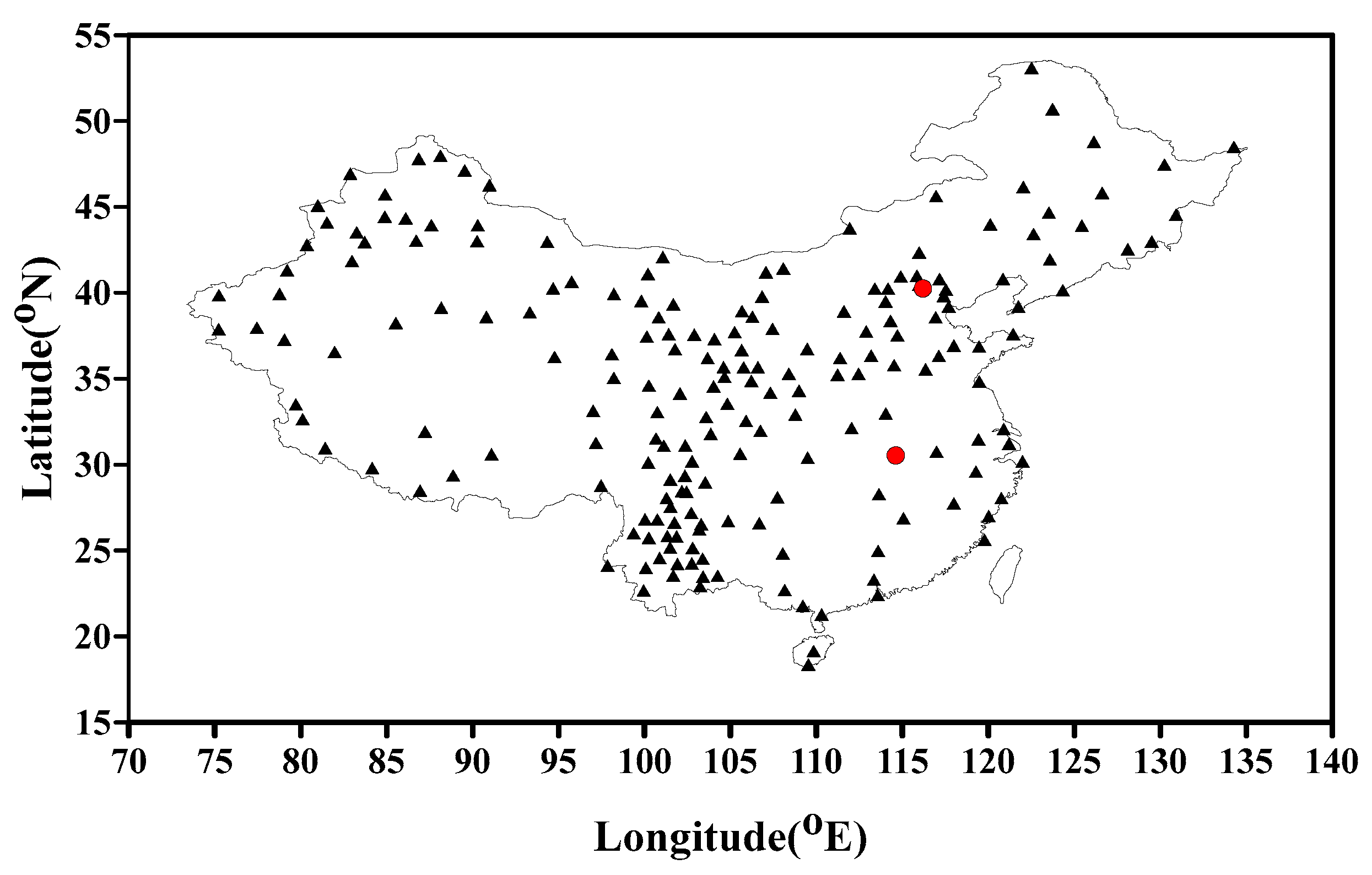
3.1. Data Sources and Preprocessing Strategy

In this work, we evaluated the performance of the ESART method when imaging IED variations using GNSS data during a geomatically quiet period on 10–12 January 2019, when the Disturbed Storm Time Index (Dst) did not exceed the absolute Dst 10 nT, and an intense geomagnetic storm period on 17–19 March, when Dst reached a minimum of −234 nT.
GNSS data from 196 reference stations belonging to the Crustal Movement Observation Network of China (CMONOC) during the periods of 10–12 January 2019 and 17–19 March 2015 were used. In addition, the ionosonde data from the Beijing (40.3°N, 116.2°E) and Wuhan (30.5°N, 114.6°E) stations were used to validate the reliability of IED retrieved from the ESART method. The ionosonde data provide an independent comparison with the electron density profiles from GNSS observations by using the tomography technique. The locations of the reference stations are shown in Figure 1.
To invert the IED, the absolute slant TEC measurements are calculated every 30 s with high accuracy using dual-frequency phase-smoothed code combination observations from the ground-based GNSS stations, and the differential code biases (DCBs) are corrected with an estimated accuracy of about 0.10 ns–0.13 ns using the two-step method developed by Li et al. [55]. In order to minimize multipath errors in GNSS data, an elevation cutoff of 20° was considered. Based on the TEC data mentioned above, the tomographic method is applied to the inversion of IED. Additionally, the International Reference Ionosphere (IRI-2016) was selected as the background to compensate for the incomplete information in the GNSS measurements for tomography.
Figure 2 shows the variation in Dst index. The top panel shows the Dst index on 17–19 March 2015, and the bottom panel shows the Dst index on 10–12 January 2019. As shown in Figure 2, the Dst index varied from −4 to 10 nT on the days in January when the geomagnetic conditions were very quiet. A strong geomagnetic storm occurred on 17–19 March 2015, at which point the fluctuation in the Dst index was much larger, with values varying from −234 nT to 45 nT.

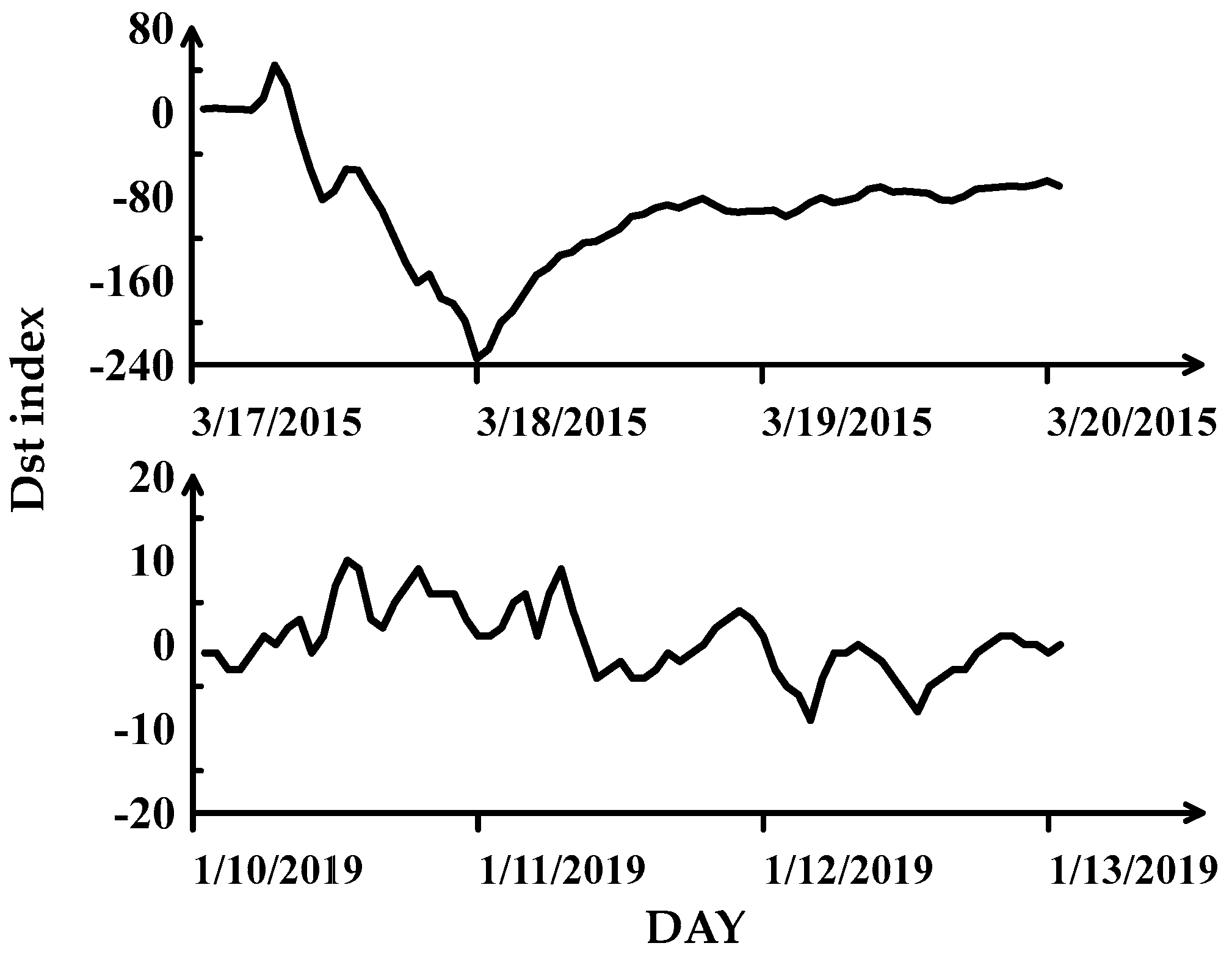
3.2. Outline of the Experiment

In this paper, the feasibility and effectiveness of the new ESART method is evaluated by comparing the IED obtained using the conventional SART method and that obtained using the IRI-2016 model. The IED observations using the three approaches are compared with ionosonde data, which are considered to be a reference in our study, and these comparisons are carried out for both quiet and disturbed ionospheric conditions. The variations in the latitude–longitude maps of the IED are also compared with those in the GNSS TEC maps during geomagnetic storms. The response of the latitude–altitude map of the IED to geomagnetic storms is also discussed. Additionally, the average root square error (RMSE) and absolute error of the reconstructed IED values are calculated and used to evaluate the performance of different reconstruction methods.
As shown in Figure 1, the reconstructed ionospheric regions cover an area from 75°E to 135°E in longitude and from 15°N to 55°N in latitude, with a height range varying from 90 to 1000 km. For both the SART and ESART methods, the horizontal resolution of each prism voxel is 2.5° × 5° lat/lon. The vertical resolution used for both methods is also the same. However, considering the large vertical variations of the ionospehric electron density gradient in the discretized ionospheric region, the vertical intervals of electron density voxels within the height ranges 90–210 km, 210–400 km, 400–700 km and 700–1000 km are set to 30, 10, 50 and 100 km, respectively. These height intervals are designed to be smaller for regions with higher electron density gradients (especially for the peak electron density region) than for regions with smaller gradients. In addition, it is assumed that the ionosphere tends to be quasi-stationary during the effective TEC measurement time of 10 min adopted for imaging the 3-D electron densities using GNSS data in this study [42,56]. The electron density is considered to be uniformly distributed within each voxel, and to remain unchanged within the short observation times.
In addition, an intervoxel smoothing strategy is adopted to fill the gaps in the GNSS data for those voxels not intersected by any GNSS rays and which depend on the initializing values of the IRI-2016 model. During the smoothing, the electron density of each voxel is redefined as a weighted sum of itself and the values of several neighboring voxels. Furthermore, a three-dimensional distance-weighted Gaussian-like boxcar average is also used, while the information of voxels with GNSS rays may be distributed to regions with data gaps. An iteration stop criterion is used, according to the mean reconstruction residual and root mean square of the TEC [52].

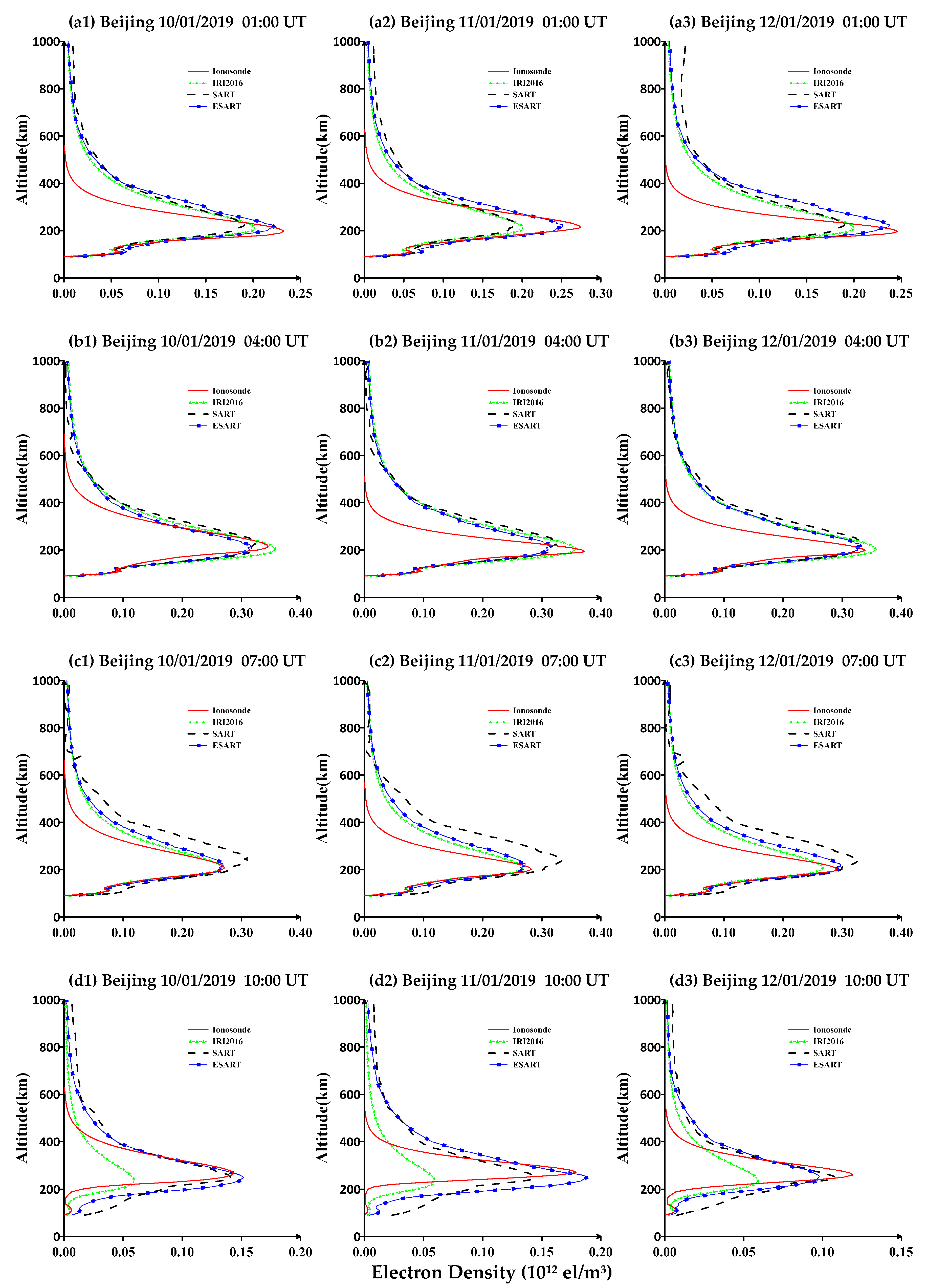
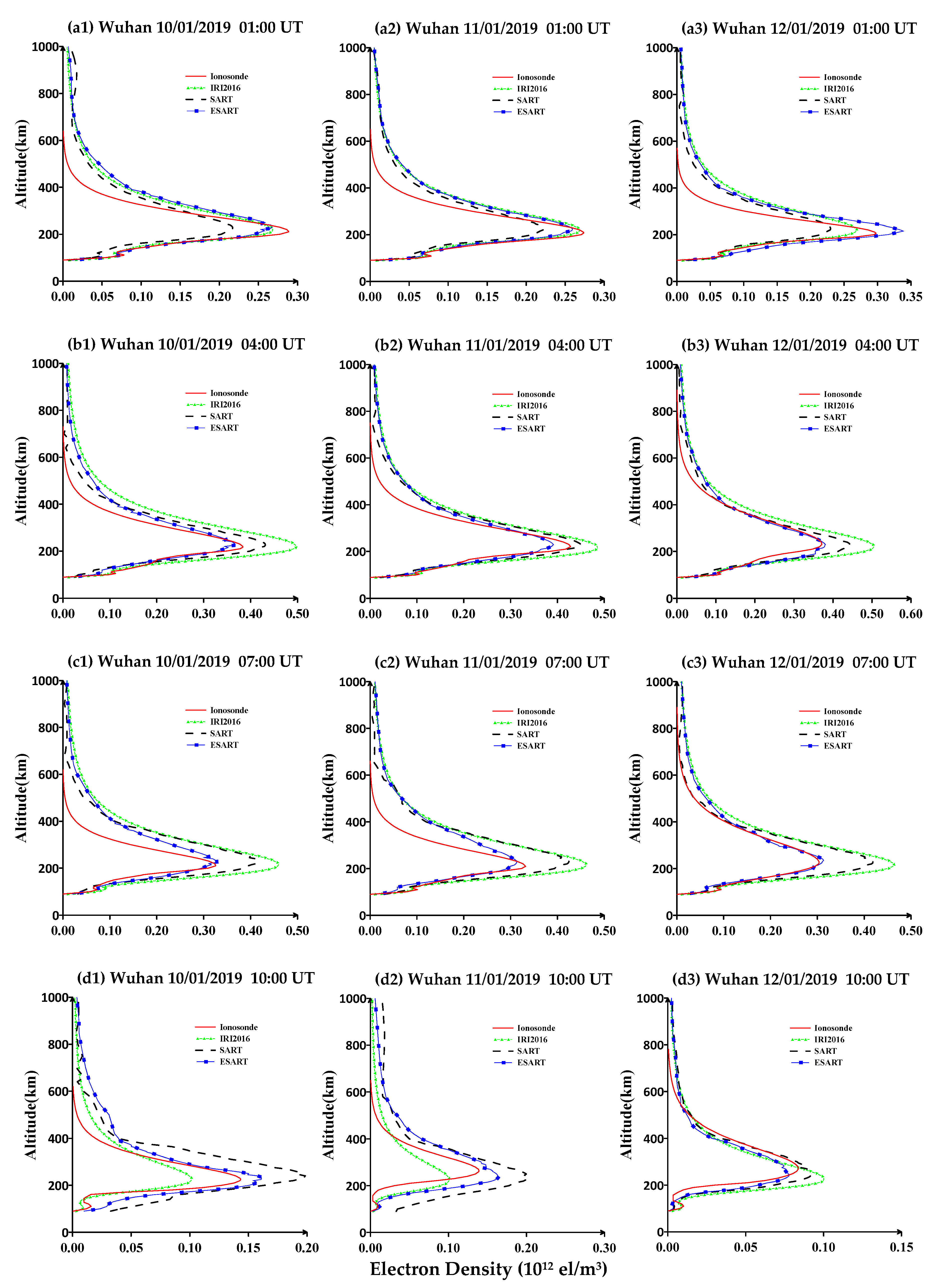
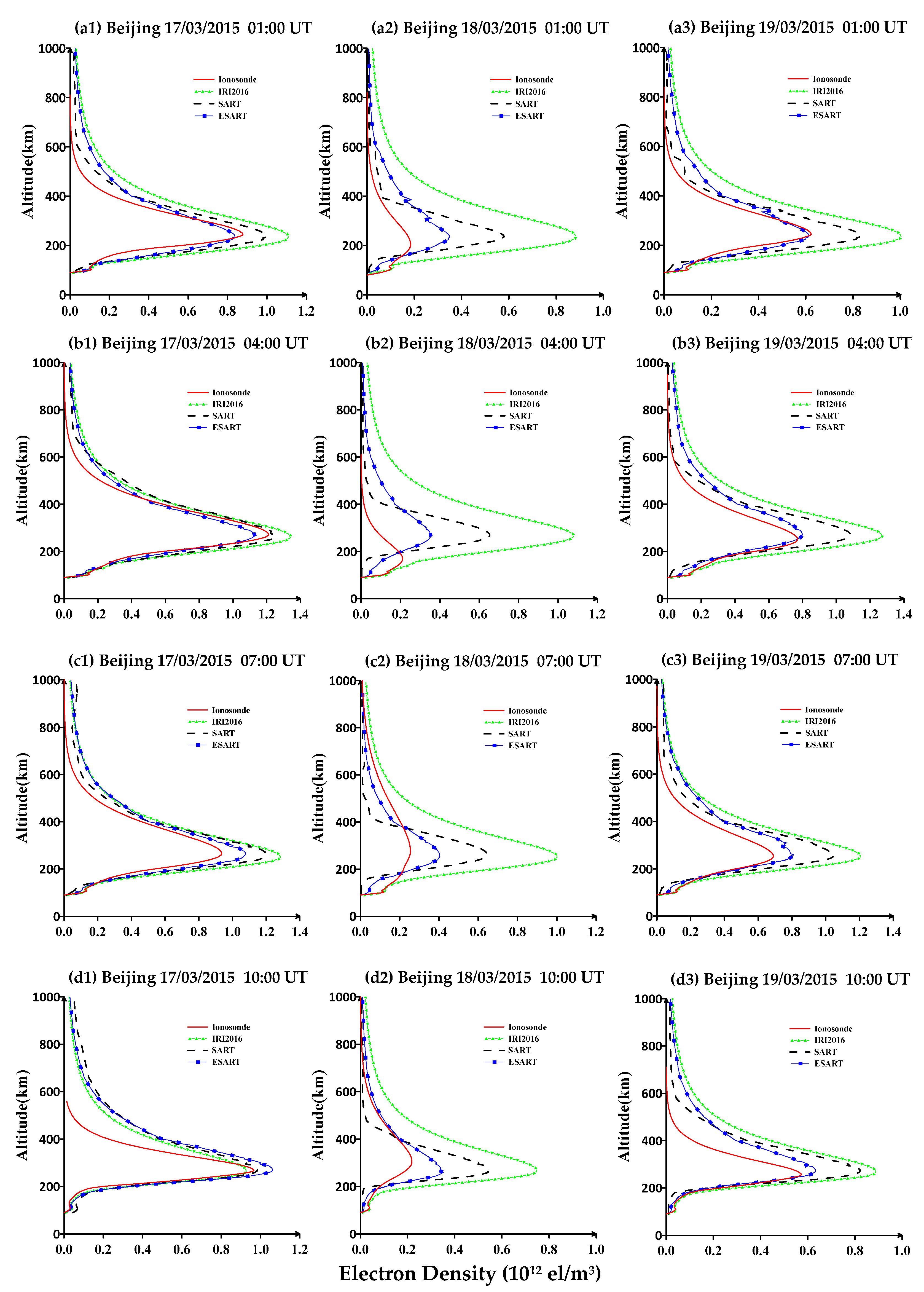
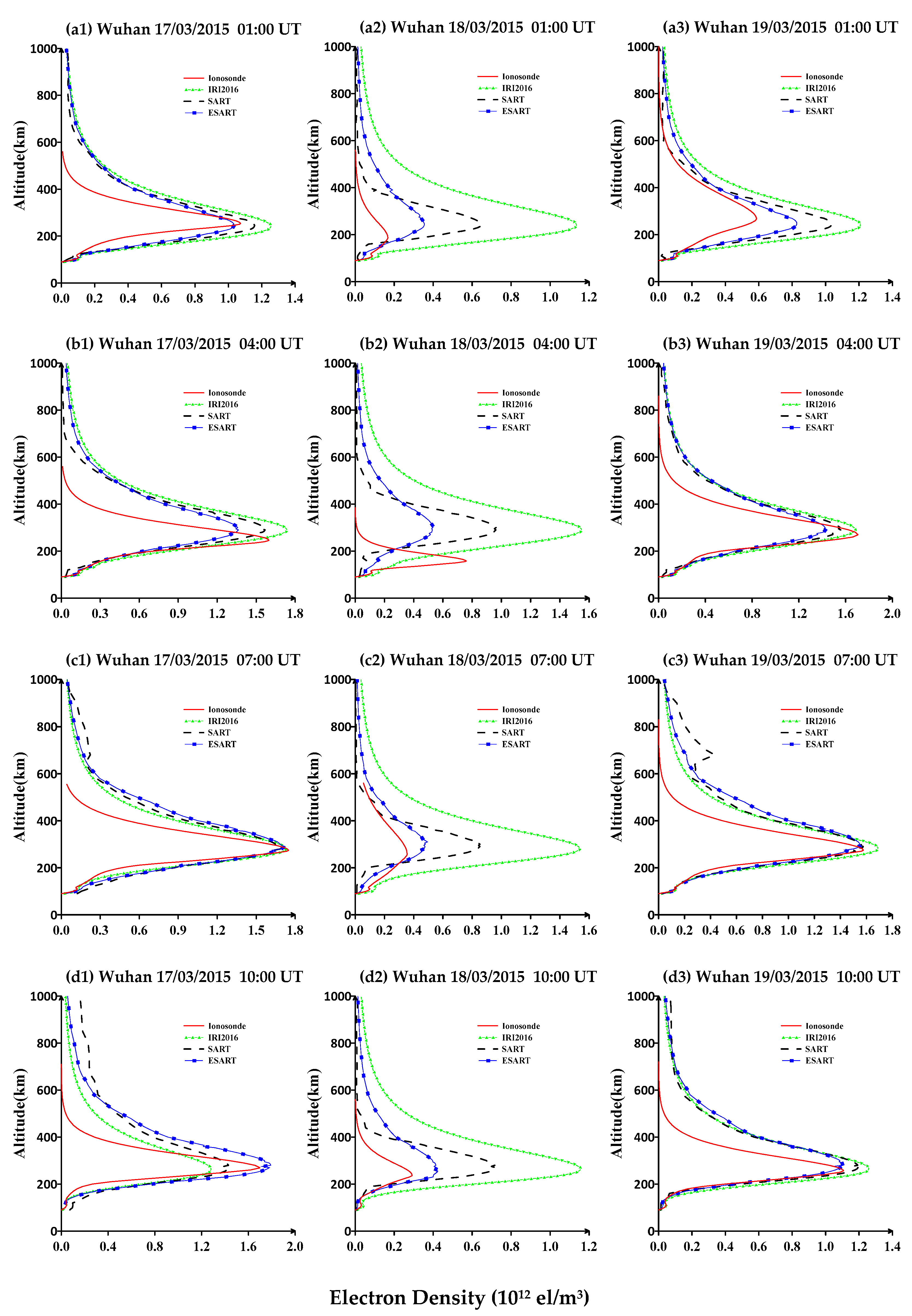
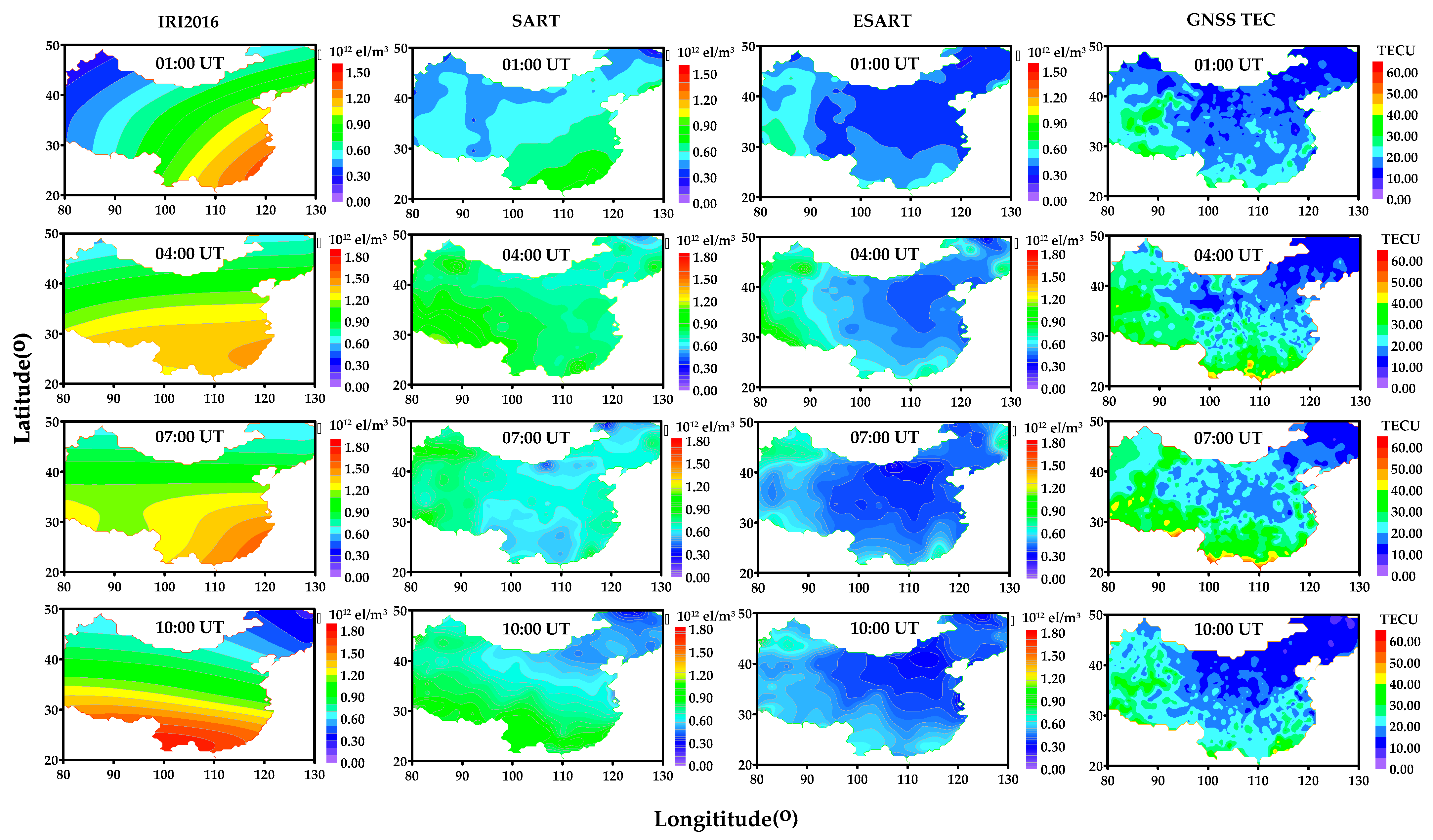
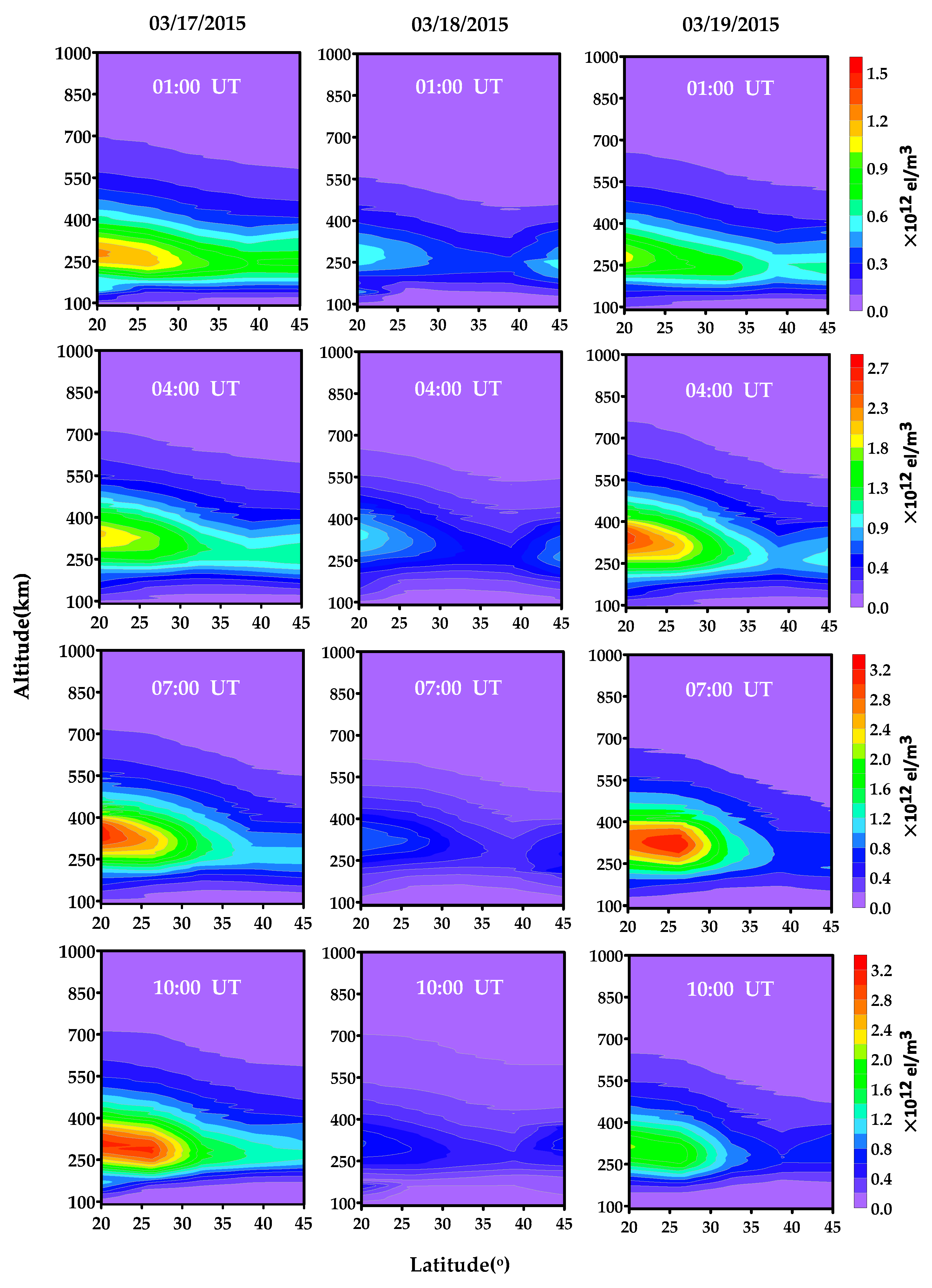
4. Results and Discussion

Figure 3, Figure 4, Figure 5 and Figure 6 present the IED profile results obtained using the conventional SART method, the ESART method and the IRI-2016 model, as well as the reference data provided by ionosonde. Each subfigure represents the IED reconstructed at different epochs, the vertical axis represents the height of the ionosphere, and the horizontal axis represents the ionospheric electron density value. Figure 3 and Figure 4 show the IED profiles obtained during 10–12 January 2019, when the geomagnetic conditions were quiet, and Figure 4 and Figure 5 show the same results during 17–19 March 2015, when strong geomagnetic storms were detected. The results from the three consecutive days are shown in the panels from left to right. The results of four time layers, i.e., 1:00 UT, 4:00 UT, 7:00 UT, and 10 UT, are shown in the rows from top to bottom, respectively.
According to Figure 3 and Figure 4, it can be clearly seen that the constructed peak electron densities (NmF2) obtained using the ESART method are generally closer to those obtained using the ionosonde than those obtained using the SART method or the IRI-2016 model. In addition, there are large discrepancies in NmF2 between the IRI-2016 model and the ionosonde results. In Figure 3(a2,a3,c1–c3) and in Figure 4 at 4:00 UT, 7:00 UT and 10:00 UT, the NmF2 values derived using the ESART method are evidently closer to those obtaind using the ionosonde than those obtained using the SART method. This indicates that the ESART method outperforms the SART method under these conditions. In addition, it can also be seen that there are small discrepancies in the NmF2 values obtained using the two tomographic methods, while the electron density profiles obtained using the IRI-2016 model are in better agreement with the ionosonde measurements.
Figure 5 and Figure 6 show that the electron density profiles obtained using the ESART method are in better agreement with the ionosonde measurements than those of the SART method or the IRI-2016 model. According to Figure 2, an intense magnetic storm occurred during 17–19 March 2015, with an observed Dst recorded on 18 March 2015 ranging from −200 nT to −82 nT. From Figure 5(a2–d2) and Figure 6(a2–d2), it is clear that the negative storm was characterized by extremely low values of IED over Beijing and Wuhan on 18 March 2015. A slightly negative storm in the mid- and high-latitudinal zone continued until 03:00 UT on 19 March, as reported in [57,58]. As mentioned above, it can be seen from Figure 5a3 and Figure 6a3 that lower IED values were recorded at 01:00 UT on 19 March at the Beijing and Wuhan stations in comparison with the corresponding IED values on 17 March. Similarly, it can be seen that the NmF2 values reconstructed using the ESART method are in better agreement with the profiles obtained from the ionosondes than those obtained using the SART method or IRI-2016.
These results suggest that ESART can generate more accurate IED profiles than the conventional SART method or the IRI-2016 model in both geomagnetically quiet conditions and during geomagnetic storms. This suggests that our approach, in which the tomographic electron density corrections are estimated based on the product of the intercept and electron density within voxels makes the assignment of corrections at different heights more effective. Therefore, a comparison of the results further proves that the ESART method provides better electron density reconstruction than the SART method or the IRI-2016 model.
It should be noted from Figure 5(a2,b2) and Figure 6(a2–d2) that the peak height of the F2 layer (hmF2) provided by the ESART and SART methods, as well as by the IRI-2016 model, deviate significantly from the electron density profiles obtained using the ionospheric ionosonde. This indicates that none of the three methods is able to accurately describe the fluctuation in hmF2 triggered by intense geomagnetic storms.
It should also be pointed out that there are obvious discrepancies in the topside part between the electron density profiles obtained from the ionosonde measurement and those derived using other methods. This is because the ionogram provides information for directly calculating the vertical electron density profile up to the peak of the ionospheric F2 layer [59], but does not provide direct information on the topside ionosphere. The profile above the peak is estimated using an alpha-Chapman function with a scale height derived from the profile shape around the F2 peak [60]. Therefore, in this paper, the focus is on the bottom side profile of the ionosphere up to the peak of the F2 layer.
Furthermore, the errors, as represented by RMSE, and the absolute differences of the three approaches compared to the ionosonde data are calculated and compared. The RMSE values and mean absolute error of the reconstructed IED profiles can be calculated by the following equations:
R M S E = I = n N e i r e c o n N e i i o n o s o n d e 2 n
Δ E = i = 1 n N e i r e c o n N e i i o n o s o n d e n
where N e i i o n o s o n d e denotes the ionospheric electron density obtained from the ionosonde measurement, N e i r e c o n represents the reconstructed bottom electron density derived from GNSS tomography, and n is the total number of the tomographic voxels along the ionospheric electron density profile.
Table 1, Table 2, Table 3 and Table 4 list the RMSE and mean absolute error of the bottom profiles of IED at the Beijing and Wuhan stations during the geomatically quiet time and during the intense geomagnetic storm, respectively.
Table 1 and Table 2 show the RMSE and absolute error of the ESART and SART methods and the IRI-2016 model on 10–12 January 2019 at the Beijing and Wuhan stations. For Beijing Station, the RMSE values of ESART, SART and IRI-2016 are 0.230, 0.283, 0.264 × 10¹¹ el/m3, respectively, and the absolute errors for the three methods are 0.173, 0.233, 0.185 × 10¹¹ el/m3, respectively. For Wuhan Station, the average RMSE of ESART, SART and IRI-2016 are 0.224, 0.387, 0.427 × 10¹¹ el/m3, respectively, and the average absolute errors are 0.176, 0.329, 0.329 × 10¹¹ el/m3, respectively, for the three methods. According to the results, the electron density obtained using the ESART method is in relatively good agreement with the ionosonde data, and Table 2 shows that the electron density of the SART method is slightly better than that obtained using the IRI-2016 model.
Table 3 and Table 4 show the RMSE and absolute errors of the ESART and SART methods, as well as the IRI-2016 model, on 17–19 March 2015 at the Beijing and Wuhan stations. For Beijing Station, the average RMSE values of IED are 0.662, 1.044, 1.482 × 10¹¹ el/m3 for ESART, SART and IRI-2016, respectively. For Wuhan Station, the average RMSE values of IED are 1.237, 1.783, 2.825 × 10¹¹ el/m3, respectively, for the three methods. The RMSE values and absolute errors of IRI-2016 are larger than the other two tomographic methods. These results also demonstrate that the RMSE and the absolute errors of the IED reconstructed using the ESART method are smaller than those when using the SART method.
On the whole, the performance of the ESART method is better than that of the IRI-2016 model, and the ESART method demonstrates an improvement in the reconstruction of IED values compared to the SART method.
As is well known, variations in NmF2 and TEC have a relatively strong correlation during the daytime. In order to further validate the effectiveness of the ESART method, in the following section, we will discuss the features among the reconstructed IED maps obtained using the IRI-2016 model, the SART and ESART methods, and the GNSS TEC maps during the geomagnetic storm.
The TEC variation maps, which characterize the evolution of the ionospheric storm in the regions of our study, were calculated using GNSS data on 17–19 March 2015. In order to analyze the responses of the electron densities obtained using the three different methods to the negative phase storm, the temporal variations in the latitude–longitude maps of the IED at an altitude of 250 km (near the altitude of peak electron density) were reconstructed using the ESART, SART, and IRI-2016 models, respectively.
Figure 7 illustrates the evolution of IED and the corresponding TEC from 01:00 UT to 10:00 UT on 18 March 2015 during the main phase of the magnetic storm. The ordinate and the abscissa are the geographic latitude and longitude. The left three columns show the IED maps obtained using IRI-2016, SART, and ESART. The color bar represents TEC in TECu. The subfigures in the fourth column are two-dimensional pseudo-color maps of GNSS TEC, and the color bar represents TEC in TECu.
In Figure 7, the storm-related ionospheric disturbances can be clearly seen, and the distinctive features of a negative ionospheric storm can be observed at 1:00 UT–10:00 UT [57,58]. From the GNSS TEC maps, it can be observed that the GNSS TECs undergo a decrease, and there is also a significant decline at 1:00–10:00 UT (9:00–18:00 LT). The GNSS TEC maps clearly depict a negative phase of the strong geomagnetic storm on 18 March 2015. However, the spatio-temporal evolution characteristics of the IED background values can be characterized using the IRI-2016 model, and no ionospheric disturbance phenomenon can be observed in the left column subfigures of Figure 7. The IED values obtained using the ESART and SART methods were obviously smaller than the background values obtained using the IRI-2016 model. In addition, the IED maps obtained using the SART and ESART methods indicated an anomalous decrease in ionospheric density, with a sharp drop in TEC values.
It should also be noted that the electron density depletion region of the IED maps obtained using the ESART method is more obvious compared to the IED maps obtained using the SART method. It can be seen that the variations in the IED maps obtained using the ESART method and the TEC maps were almost synchronous, which demonstrates the effectiveness of the ESART method proposed in this paper.
According to related reports [57,58], a weakly positive TEC disturbance occurred at 08:00 UT in 45°N–60°N zone on 17 March 2015. One hour later, the positive TEC disturbances extended to 30°N. In addition, the distinct mid-latitude zones of increased TEC were then observed at 10:00–13:00 UT. Figure 8 presents latitude–altitude maps of ionospheric electron density at 1:00 UT–10:00 UT on 17–19 March 2015. In the left subfigures, it can be seen that there is a weak positive disturbance in the IED, with an enhanced electron density phenomenon at 10:00 UT compared to other time layers on 17 March 2015. In the middle subfigures, it can be clearly seen that very low values of IED on 18 March were observed compared to IED on 17 March and 19 March, and there is a distinct negative storm phenomenon in the 20°N–45°N zone. In addition, at 01:00 UT and 04:00 UT on March 19, the values of IED between about 200 km–300 km in the 35°N–45°N zone are slightly smaller than the IED values on 17 March. These results are consistent with from the reports in [57,58], demonstrating the ability of the proposed ESART method to perform imaging of the ionosphere.
It should be noted that fluctuations in the hmF2 cannot be observed in Figure 8, which is consistent with the phenomenon reflected in Figure 5(a2,b2) and Figure 6(a2–d2). In other words, the ESART method is not able to reveal the fluctuations in hmF2 triggered by intense geomagnetic storms, which is also an issue that needs to be further studied in future.

5. Conclusions

This paper proposed the ESART method for imaging three-dimensional electron densities using an ionospheric tomography technique. In the ESART method, the product of the intersection length with the electron density is introduced into the corresponding voxel, instead of the length of the ray–voxel intersection, while the differences between the measured and calculated TEC are also reasonably redistributed among the ray–voxels. This new method ensures that the actual correction of the electron density in a voxel matches the contribution of the corresponding voxel to the GNSS TEC by accounting for the contribution of a voxel to the GNSS TEC in terms of both its geometric contribution and the contribution of its electron density.
The ESART method was evaluated by comparing it to the SART method and the IRI-2016 model under geomagnetically quiet conditions on 10–11 January 2019, as well as during a geomagnetic storm period on 17–19 March 2015. Data from an ionosonde were used as a reference in this study. The results show that the constructed electron density obtained using the ESART method was generally closer to the reference data from the ionosonde than that of the SART method or the IRI-2016 model (especially for the NmF2), confirming the effectiveness of the proposed ESART method.
Furthermore, we presented latitude–longitude pictures of the IED during the intense geomagnetic storm, displaying the spatial and temporal variations, as well as the variations in latitude profile with altitude, on 17–19 March 2015, demonstrating the great potential of the proposed ESART method to provide high-quality IED reconstruction.
It should be noted that the results presented in this study, and which demonstrate the feasibility of the new method, are preliminary. The top plasma density obtained using the ESART method should be carefully evaluated using COSMIC and Swarm data, and the data span was relatively short compared to the 11-year periodic solar variation activity. Therefore, the next step of research will focus on using more data to explore the applicability of the ESART method in the GNSS application field. In addition, the theoretical background for the ESART method has not yet been properly investigated; nevertheless, the practical results suggest that the method works as expected.

Author Contributions

Conceptualization, Y.L. (Yuanliang Long) and X.H.; methodology, X.H.; software, Y.L. (Yuanliang Long) and H.L.; validation, H.L. and W.S.; formal analysis, Y.L. (Yuanliang Long) and Y.L. (Ying Li); investigation, Y.L. (Yuanliang Long) and X.H; resources, X.H.; data curation, X.H.; writing—original draft preparation, Y.L. (Yuanliang Long); writing—review and editing, Y.L. (Ying Li); visualization, W.S.; supervision, X.H.; project administration, X.H.; funding acquisition, X.H. All authors have read and agreed to the published version of the manuscript.

Funding

This research was funded by National Natural Science Foundation of China (NO. 42074045, 42004027 and 41574033).

Data Availability Statement

GNSS data in this study is provided by China Earthquake Networks Center, National Earthquake Data Center (http://data.earthquake.cn, accessed on 6 November 2020) and by the Chinese Meridian Project (https://data.meridianproject.ac.cn/, accessed on 6 November 2020). The precise orbit and clock offset products were provided by IGS (https://cddis.nasa.gov/archive/gps/products/, accessed on 6 January 2023). Ionosonde data were provided by Beijing National Observatory of Space Environment, Institute of Geology and Geophysics Chinese Academy of Sciences through the Geophysics center, National Earth System Science Data Center (http://wdc.geophys.ac.cn, accessed on 13 April 2020). Dst index was provided by World Data Center for Geomagnetism, Kyoto University (http://wdc.kugi.kyoto-u.ac.jp/dstdir/index.html, accessed on 9 January 2023).

Acknowledgments

We acknowledge the Crustal Movement Observation Network of China (CMONOC) and the Chinese Meridian Project for providing access to GNSS data. We also acknowledge the National Earth System Science Data Center for providing access to ionosonde data, and Kyoto University for providing access to Dst index. The IRI-2016 Fortran source code can be downloaded from the IRI official website (http://www.irimodel.org, accessed on 9 January 2023).

Conflicts of Interest

The authors declare no conflict of interest.

References

  1. Austen, J.R.; Franke, S.J.; Liu, C.H. Ionospheric imaging using computerized tomography. Radio Sci. 1988, 23, 299–307. [Google Scholar] [CrossRef]
  2. Bust, G.S.; Mitchell, C.N. History, current state, and future directions of ionospheric imaging. Rev. Geophys. 2008, 46, 1–23. [Google Scholar] [CrossRef]
  3. Hernández-Pajares, M.; Juan, J.M.; Sanz, J.; Colombo, O.L. Application of ionospheric tomography to real-time GPS carrier-phase ambiguities Resolution, at scales of 400–1000 km and with high geomagnetic activity. Geophys. Res. Lett. 2000, 27, 2009–2012. [Google Scholar] [CrossRef] [Green Version]
  4. Allain, D.J.; Mitchell, C.N. Ionospheric delay corrections for single-frequency GPS receivers over Europe using tomographic mapping. GPS Solut. 2009, 13, 141–151. [Google Scholar] [CrossRef]
  5. Kong, J.; Lulu, S.; Zhou, C.; Yao, Y.; An, J.; Wang, Z. An Improved Computerized Ionospheric Tomography Model Fusing 3-D Multisource Ionospheric Data Enabled Quantifying the Evolution of Magnetic Storm. IEEE Trans. Geosci. Remote Sens. 2020, 59, 3725–3736. [Google Scholar] [CrossRef]
  6. Mei, D.; Ren, X.; Liu, H.; Le, X.; Xiong, S.; Zhang, X. Global Three-Dimensional Ionospheric Tomography by Combination of Ground-Based and Space-Borne GNSS Data. Space Weather 2023, 21, e2022SW003368. [Google Scholar] [CrossRef]
  7. Liu, Z.Z.; Skone, S.; Gao, Y. Assessment of ionosphere tomographic modeling performance using GPS data during the October 2003 geomagnetic storm event. Radio Sci. 2006, 41, RS1007. [Google Scholar] [CrossRef] [Green Version]
  8. Hernández-Pajares, M.; Juan, J.M.; Sanz, J.; Aragón-Àngel, À.; García-Rigo, A.; Salazar, D.; Escudero, M. The ionosphere: Effects, GPS modeling and the benefits for space geodetic techniques. J. Geod. 2011, 85, 887–907. [Google Scholar] [CrossRef]
  9. Schunk, R.W.; Scherliess, L.; Sojka, J.J. Recent approaches to modeling ionospheric weather. Adv. Space Res. 2003, 31, 819–828. [Google Scholar] [CrossRef]
  10. Wen, D.; Yuan, Y.; Ou, J.; Zhang, K. Ionospheric Response to the Geomagnetic Storm on 21 August 2003 Over China Using GNSS-Based Tomographic Technique. IEEE Trans. Geosci. Remote Sens. 2010, 48, 3212–3217. [Google Scholar] [CrossRef]
  11. Muella, M.; de Paula, E.; Mitchell, C.; Kintner, P.; Paes, R.; Batista, I. Tomographic imaging of the equatorial and low-latitude ionosphere over central-eastern Brazil. Earth Planets Space 2011, 63, 129–138. [Google Scholar] [CrossRef] [Green Version]
  12. Yao, Y.; Zhai, C.; Kong, J.; Zhao, Q.; Zhao, C. A modified three-dimensional ionospheric tomography algorithm with side rays. GPS Solut. 2018, 22, 107. [Google Scholar] [CrossRef]
  13. Jin, S.; Li, D. 3-D ionospheric tomography from dense GNSS observations based on an improved two-step iterative algorithm. Adv. Space Res. 2018, 62, 809–820. [Google Scholar] [CrossRef]
  14. Prol, F.; Camargo, P. Review of tomographic reconstruction methods of the ionosphere using GNSS. Rev. Bras. Geofísica 2015, 33, 445. [Google Scholar] [CrossRef] [Green Version]
  15. Ren, X.; Mei, D.; Zhang, X.; Freeshah, M.; Xiong, S. Electron Density Reconstruction by Ionospheric Tomography From the Combination of GNSS and Upcoming LEO Constellations. J. Geophys. Res. Space Phys. 2021, 126, e2020JA029074. [Google Scholar] [CrossRef]
  16. Yin, P.; Mitchell, C.N.; Spencer, P.S.J.; Foster, J.C. Ionospheric electron concentration imaging using GPS over the USA during the storm of July 2000. Geophys. Res. Lett. 2004, 31, 1–4. [Google Scholar] [CrossRef]
  17. Huo, X.; Yuan, Y.; Ou, J.; Li, Y.; Li, Z.; Wang, N. A new ionospheric tomographic algorithm taking into account the variation of the ionosphere. Chin. J. Geophys. 2016, 59, 2393–2401. [Google Scholar] [CrossRef]
  18. Yu, J.; Zhu, Y.; Dai, Y.; Zhu, H.; Huang, Y.; Wu, L.; Sun, Y. Dual Empirical Orthogonal Functions Restrained Tomographic Model for Ionosphere Imaging. IEEE Trans. Geosci. Remote Sens. 2022, 60, 4110512. [Google Scholar] [CrossRef]
  19. Lu, W.; Ma, G.; Wan, Q. A Review of Voxel-Based Computerized Ionospheric Tomography with GNSS Ground Receivers. Remote Sens. 2021, 13, 3432. [Google Scholar] [CrossRef]
  20. Prol, F.; Pajares, M.; Muella, M.; Camargo, P. Tomographic Imaging of Ionospheric Plasma Bubbles Based on GNSS and Radio Occultation Measurements. Remote Sens. 2018, 10, 1529. [Google Scholar] [CrossRef] [Green Version]
  21. Prol, F.; Kodikara, T.; Hoque, M.; Borries, C. Global-Scale Ionospheric Tomography During the 17 March 2015 Geomagnetic Storm. Space Weather 2021, 19, e2021SW002889. [Google Scholar] [CrossRef]
  22. Feng, J.; Zhou, Y.; Zhou, Y.; Gao, S.; Zhou, C.; Tang, Q.; Liu, Y. Ionospheric response to the 17 March and 22 June 2015 geomagnetic storms over Wuhan region using GNSS-based tomographic technique. Adv. Space Res. 2020, 67, 111–121. [Google Scholar] [CrossRef]
  23. Nesterov, I.; Kunitsyn, V. GNSS radio tomography of the ionosphere: The problem with essentially incomplete data. Adv. Space Res. 2011, 47, 1789–1803. [Google Scholar] [CrossRef]
  24. Raymond, T.D.; Franke, S.J.; Yeh, K.C. Ionospheric tomography: Its limitations and reconstruction methods. J. Atmos. Sol. Terr. Phys. 1994, 56, 637–657. [Google Scholar] [CrossRef]
  25. Wen, D.; Yuan, Y.; Ou, J.; Zhang, K.; Liu, K. A Hybrid Reconstruction Algorithm for 3-D Ionospheric Tomography. IEEE Trans. Geosci. Remote Sens. 2008, 46, 1733–1739. [Google Scholar] [CrossRef] [Green Version]
  26. Yao, Y.; Tang, J.; Kong, J.; Liang, Z.; Zhang, S. Application of hybrid regularization method for tomographic reconstruction of midlatitude ionospheric electron density. Adv. Space Res. 2013, 52, 2215–2225. [Google Scholar] [CrossRef]
  27. Zhou, C.; Fremouw, E.J.; Sahr, J.D. Optimal truncation criterion for application of singular value decomposition to ionospheric tomography. Radio Sci. 1999, 34, 155–166. [Google Scholar] [CrossRef]
  28. Bhuyan, K.; Singh, S.; Bhuyan, P. Tomographic reconstruction of the ionosphere using generalized singular value decomposition. Curr. Sci. 2002, 83, 1117–1120. [Google Scholar]
  29. Erturk, O.; Arikan, O.; Arikan, F. Tomographic reconstruction of the ionospheric electron density as a function of space and time. Adv. Space Res. 2009, 43, 1702–1710. [Google Scholar] [CrossRef]
  30. Hong, J.; Kim, Y.; Chung, J.-K.; Ssessanga, N.; Kwak, Y.-S. Tomography Reconstruction of Ionospheric Electron Density with Empirical Orthonormal Functions Using Korea GNSS Network. J. Astron. Space Sci. 2017, 34, 7–17. [Google Scholar] [CrossRef] [Green Version]
  31. Norberg, J.; Virtanen, I.; Roininen, L.; Vierinen, J.; Orispää, M.; Kauristie, K.; Lehtinen, M. Bayesian statistical ionospheric tomography improved by incorporating ionosonde measurements. Atmos. Meas. Tech. 2016, 9, 1859–1869. [Google Scholar] [CrossRef] [Green Version]
  32. Norberg, J.; Vierinen, J.; Roininen, L.; Orispää, M.; Kauristie, K.; Rideout, W.; Coster, A.; Lehtinen, M. Gaussian Markov Random Field Priors in Ionospheric 3-D Multi-Instrument Tomography. IEEE Trans. Geosci. Remote Sens. 2018, 56, 7009–7021. [Google Scholar] [CrossRef] [Green Version]
  33. Zhao, J.; Tang, Q.; Zhou, C.; Zhao, Z.; Wei, F. Three-dimensional ionospheric tomography based on compressed sensing. GPS Solut. 2023, 27, 90. [Google Scholar] [CrossRef]
  34. Aa, E.; Zhang, S.R.; Erickson, P.J.; Wang, W.; Coster, A.J.; Rideout, W. 3-D Regional Ionosphere Imaging and SED Reconstruction With a New TEC-Based Ionospheric Data Assimilation System (TIDAS). Space Weather 2022, 20, e2022SW003055. [Google Scholar] [CrossRef]
  35. Norberg, J.; Roininen, L.; Vierinen, J.; Amm, O.; McKay-Bukowski, D.; Lehtinen, M. Ionospheric tomography in Bayesian framework with Gaussian Markov random field priors. Radio Sci. 2015, 50, 138–152. [Google Scholar] [CrossRef] [Green Version]
  36. Norberg, J.; Kaki, S.; Roininen, L.; Mielich, J.; Virtanen, I.I. Model-Free Approach for Regional Ionospheric Multi-Instrument Imaging. J. Geophys. Res. Space Phys. 2023, 128, e2022JA030794. [Google Scholar] [CrossRef]
  37. Raymund, T.D.; Austen, J.R.; Franke, S.J.; Liu, C.H.; Klobuchar, J.A.; Stalker, J.R. Application of computerized tomography to the investigation of ionospheric structures. Radio Sci. 1990, 25, 771–789. [Google Scholar] [CrossRef]
  38. Das, S.; Shukla, A. Two-dimensional Ionospheric Tomography over the Low Latitude Indian Region: An Inter-comparison of ART and MART Algorithms. Radio Sci. 2011, 46, 1–13. [Google Scholar] [CrossRef]
  39. Pryse, S.E.; Kersley, L. A preliminary experimental test of ionospheric tomography. J. Atmos. Terr. Phys. 1992, 54, 1007–1012. [Google Scholar] [CrossRef]
  40. Yao, Y.; Zhai, C.; Kong, J.; Zhao, C.; Luo, Y.; Liu, L. An improved constrained simultaneous iterative reconstruction technique for ionospheric tomography. GPS Solut. 2020, 24, 68. [Google Scholar] [CrossRef]
  41. Nandi, S.; Bandyopadhyay, B. Study of low-latitude ionosphere over Indian region using simultaneous algebraic reconstruction technique. Adv. Space Res. 2014, 55, 545–553. [Google Scholar] [CrossRef]
  42. Mitchell, C.; Kersley, L.; Heaton, J.; Pryse, S. Determination of the vertical electron-density profile in ionospheric tomography: Experimental results. Ann. Geophys. 1997, 15, 747–752. [Google Scholar] [CrossRef]
  43. Pryse, S.E.; Kersley, L.; Mitchell, C.N.; Spencer, P.S.J.; Williams, M.J. A comparison of reconstruction techniques used in ionospheric tomography. Radio Sci. 1998, 33, 1767–1779. [Google Scholar] [CrossRef]
  44. Wen, D.; Yuan, Y.; Ou, J.; Huo, X.; Zhang, K. Three-dimensional ionospheric tomography by an improved algebraic reconstruction technique. GPS Solut. 2007, 11, 251–258. [Google Scholar] [CrossRef]
  45. Zheng, D.; Wusheng, H.; Nie, W. Multiscale ionospheric tomography. GPS Solut. 2014, 19, 579–588. [Google Scholar] [CrossRef]
  46. Saito, S.; Suzuki, S.; Yamamoto, M.; Chen, C.-H.; Saito, A. Real-Time Ionosphere Monitoring by Three-Dimensional Tomography over Japan. Navigation 2017, 64, 495–504. [Google Scholar] [CrossRef] [Green Version]
  47. Zheng, D.; Li, P.; He, J.; Hu, W.; Li, C. Research on ionospheric tomography based on variable pixel height. Adv. Space Res. 2016, 57, 1847–1858. [Google Scholar] [CrossRef]
  48. Hobiger, T.; Kondo, T.; Koyama, Y. Constrained Simultaneous Algebraic Reconstruction Technique (C-SART)—A new and simple algorithm applied to ionospheric tomography. Earth Planets Space 2008, 60, 727–735. [Google Scholar] [CrossRef] [Green Version]
  49. Wen, D.; Liu, S.; Tang, P. Tomographic reconstruction of ionospheric electron density based on constrained algebraic reconstruction technique. GPS Solut. 2010, 14, 375–380. [Google Scholar] [CrossRef]
  50. Wen, D.; Wang, Y.; Norman, R. A new two-step algorithm for ionospheric tomography solution. GPS Solut. 2012, 16, 89–94. [Google Scholar] [CrossRef]
  51. Zheng, D.; Yao, Y.; Nie, W.; Yang, W.; Wusheng, H.; Minsi, A.; Hongwei, Z. An Improved Iterative Algorithm for Ionospheric Tomography Reconstruction by Using the Automatic Search Technology of Relaxation Factor. Radio Sci. 2018, 53, 1051–1066. [Google Scholar] [CrossRef] [Green Version]
  52. Stolle, C. Three-Dimensional Imaging of Ionospheric Electron Density Fields Using GPS Observations at the Ground and Onboard the CHAMP Satellite. Ph.D. Thesis, Universität Leipzig, Institut für Meteorologie, Leipzig, Germany, 2005. [Google Scholar]
  53. Andersen, A.; Kak, A.C. Simultaneous Algebraic Reconstruction Technique (SART): A Superior Implementation of the ART Algorithm. Ultrason. Imaging 1984, 6, 81–94. [Google Scholar] [CrossRef]
  54. Jiang, M.; Wang, G. Convergence of the Simultaneous Algebraic Reconstruction Technique (SART). IEEE Trans. Image Process. A Publ. IEEE Signal Process. Soc. 2003, 12, 957–961. [Google Scholar] [CrossRef] [PubMed]
  55. Li, Z.; Yuan, Y.; Li, H.; Ou, J.; Huo, X. Two-Step Method for the Determination of the Differential Code Biases of COMPASS Satellites. J. Geod. 2012, 86, 1059–1076. [Google Scholar] [CrossRef]
  56. Watermann, J.; Bust, G.; Thayer, J.; Neubert, T.; Coker, C. Mapping plasma structures in the high-latitude ionosphere using beacon satellite, incoherent scatter radar and ground-based magnetometer observations. Ann. Geophys. 2009, 45, 177–189. [Google Scholar] [CrossRef]
  57. Polekh, N.; Zolotukhina, N.; Kurkin, V.I.; Zherebtsov, G.; Shi, J.; Wang, G.; Wang, Z. Dynamics of ionospheric disturbances during the 17-19 March 2015 geomagnetic storm over East Asia. Adv. Space Res. 2017, 60, 2464–2476. [Google Scholar] [CrossRef]
  58. Sun, W.J.; Ning, B.Q.; Zhao, B.Q.; Li, G.; Hu, L.; Chang, S.M. Analysis of ionospheric features in middle and low latitude region of China during the geomagnetic storm in March 2015. Chin. J. Geophys. 2017, 60, 1–10. [Google Scholar]
  59. Liu, L.; Wan, W.; Ning, B. A study of the ionogram derived effective scale height around the ionospheric hmF2. Ann. Geophys. 2006, 24, 851–860. [Google Scholar] [CrossRef] [Green Version]
  60. Huang, X.; Reinisch, B.W. Vertical electron content from ionograms in real time. Radio Sci. 2001, 36, 335–342. [Google Scholar] [CrossRef] [Green Version]
Figure 1. Distribution of GNSS stations and ionosonde stations used in this work. (The black triangles represent GNSS stations, and the red circles represent the ionosonde stations.).
Remotesensing 15 02939 g001
Figure 2. Variation in Dst index on 17–19 March 2015 and 10–12 January 2019.
Remotesensing 15 02939 g002
Figure 3. Comparison of electron density profiles over Beijing Station at 01:00 UT (a1a3), 04:00 UT (b1b3), 07:00 UT (c1c3), and 10:00 UT (d1d3) on 10 January (left panel), 11 January (middle panel), 12 January (right panel), 2019. The red curve is the ionosonde data, the blue dotted line is the ESART reconstruction result, the black dashed line is the SART reconstruction result, and the green line is the IRI-2016 model.
Remotesensing 15 02939 g003
Figure 4. Comparison of electron density profiles over Wuhan Station at 01:00 UT (a1a3), 04:00 UT (b1b3), 07:00 UT (c1c3), and 10:00 UT (d1d3) on 10 January (left panel), 11 January (middle panel), 12 January (right panel), 2019. The red curve is the ionosonde data, the blue dotted line is the ESART reconstruction result, the black dashed line is the SART reconstruction result, and the green line is the IRI-2016 model.
Remotesensing 15 02939 g004
Figure 5. Comparison of electron density profiles over Beijing Station at 01:00 UT (a1a3), 04:00 UT (b1b3), 07:00 UT (c1c3), and 10:00 UT (d1d3) on 17 March (left panel), 18 March (middle panel), 19 March (right panel), 2015. The red curve is the ionosonde data, the blue dotted line is the ESART reconstruction result, the black dashed line is the SART reconstruction result, and the green line is the IRI-2016 model.
Remotesensing 15 02939 g005
Figure 6. Comparison of electron density profiles over Wuhan Station at 01:00 UT (a1a3), 04:00 UT (b1b3), 07:00 UT (c1c3), and 10:00 UT (d1d3) on 17 March (left panel), 18 March (middle panel), 19 March (right panel), 2015. The red curve is the ionosonde data, the blue dotted line is the ESART reconstruction result, the black dashed line is the SART reconstruction result, and the green line is the IRI-2016 model.
Remotesensing 15 02939 g006
Figure 7. IED maps at an altitude of 250 km obtained using the IRI-2016 model, the SART method, and the ESART method, and the corresponding GNSS TEC maps at 01:00 UT–10:00 UT on 18 March 2015. The three left columns are the IED maps obtained using IRI-2016, SART, and ESART. The color bar represents TEC in TECu. The subfigures in the fourth column are two-dimensional pseudo-color maps of GNSS TEC, and the color bar represents TEC in TECu.
Remotesensing 15 02939 g007
Figure 8. The latitude–altitude profiles of the IED along the 110 °E meridian at 1:00–10:00 UT on 17–19 March 2015. The left columns are the IED maps on 17 March, the middle columns are the IED maps on 18 March, and the right columns are the IED maps on 19 March. The color bar to the right of the subfigures marks the electron density in 1012 el/m3 unit.
Remotesensing 15 02939 g008
Table 1. Errors for the reconstructed IED values below the peak altitude of the ionospheric F2-layer when using the SART and ESART methods and the IRI-2016 model on 10–12 January 2019 at Beijing Station (Unit: 1011 el/m3).
DayRMESΔE
ESARTSARTIRI-2016ESARTSARTIRI-2016
10/01/20190.248 0.263 0.257 0.183 0.216 0.181
11/01/20190.237 0.276 0.254 0.175 0.234 0.169
12/01/20190.206 0.309 0.282 0.162 0.248 0.204
Ave0.230 0.283 0.264 0.173 0.233 0.185
Table 2. Errors for the reconstructed IED values below the peak altitude of the ionospheric F2-layer when using the SART and ESART methods and the IRI-2016 model on 10–12 January 2019 at Wuhan Station (Unit: 1011 el/m3).
DayRMESΔE
ESARTSARTIRI-2016ESARTSARTIRI-2016
10/01/20190.207 0.428 0.442 0.161 0.373 0.358
11/01/20190.233 0.397 0.376 0.182 0.341 0.292
12/01/20190.231 0.337 0.462 0.186 0.273 0.338
Ave0.224 0.387 0.427 0.176 0.329 0.329
Table 3. Errors for the reconstructed IED values below the peak altitude of the ionospheric F2-layer when using the SART and ESART methods and the IRI-2016 model on 17–19 March 2015 at Beijing Station (Unit: 1011 el/m3).
DayRMESΔE
ESARTSARTIRI-2016ESARTSARTIRI-2016
17/03/20150.662 1.044 1.482 0.519 0.869 1.132
18/03/20150.774 1.558 2.806 0.614 1.208 2.081
19/03/20150.526 1.200 1.799 0.412 0.983 1.410
Ave0.662 1.044 1.482 0.519 0.869 1.132
Table 4. Errors for the reconstructed IED values below the peak altitude of the ionospheric F2-layer when using the SART and ESART methods and the IRI-2016 model on 17–19 March 2015 at Wuhan Station (Unit: 1011 el/m3).
DayRMESΔE
ESARTSARTIRI-2016ESARTSARTIRI-2016
17/03/20151.602 1.816 2.096 1.151 1.383 1.479
18/03/20151.117 2.198 4.329 0.870 1.658 3.258
19/03/20150.992 1.334 2.051 0.740 1.008 1.567
Ave1.237 1.783 2.825 0.920 1.350 2.101
Disclaimer/Publisher’s Note: The statements, opinions and data contained in all publications are solely those of the individual author(s) and contributor(s) and not of MDPI and/or the editor(s). MDPI and/or the editor(s) disclaim responsibility for any injury to people or property resulting from any ideas, methods, instructions or products referred to in the content.

