Mapping Paddy Rice Planting Area in Dongting Lake Area Combining Time Series Sentinel-1 and Sentinel-2 Images

Abstract

Accurate and timely acquisition of cropping intensity and spatial distribution of paddy rice is not only an important basis for monitoring growth and predicting yields, but also for ensuring food security and optimizing the agricultural production management system of cropland. However, due to the monsoon climate in southern China, it is cloudy and rainy throughout the year, which makes it difficult to obtain accurate information on rice cultivation based on optical time series images. Conventional image synthesis is prone to omission or redundancy of spectral and temporal features that are potentially important for rice-growth identification, making it difficult to determine the optimal features for high-precision mapping of paddy rice. To address these issues, we develop a method to granulate the effective use interval of classification features by extracting phenological signatures of rice to obtain cost-effective and highly accurate mapping results. Two steps are involved in this method: (1) analyzing the information on various features (spectra, polarization, and seasonal regularity) to identify three key phenological periods throughout the lifespan of paddy rice; (2) identifying the features with the highest class separation between paddy rice, non-paddy crops, and wetlands under different phenological stages; and (3) removing redundant features to retain the optimal feature combinations. Subsequently, the obtained feature sets are used as input data for the random forest classifier. The results showed that the overall accuracy of the identified rice results was 95.44% with F1 scores above 93% for both single- and double-cropping rice. Meanwhile, the correlation coefficient of our mapped rice area compared with the official statistics of rice area at county and district levels was 0.86. In addition, we found that combining Sentinel-1 and Sentinel-2 images for rice recognition was better than using Sentinel-1 or Sentinel-2 alone, and the classification accuracy was improved by 5.82% and 2.39%, which confirms that the synergistic Sentinel-1 and Sentinel-2 data can effectively overcome the problem of missing optical images caused by clouds and rain. Our study demonstrates the potential of distinguishing mixed rice-cropping systems in subtropical regions with fragmented rice-field distribution in a cloudy and rainy environment, and also provides a basis for the rational layout of rice production and improvement of cultivation systems.

1. Introduction

As one of the most important staple foods for more than half of the world’s population [1], paddy rice is fundamental to achieving the goal UN of ending hunger by 2030 as outlined in the 17 Sustainable Development Goals (SDGs), and not only plays a key role in global food security [2], but also in environmental issues, such as greenhouse gas (CH₄) emissions [3,4], freshwater uses [5,6,7], soil quality improvements [8,9], and wetland loss [10]. However, under the combined effects of global climate change, population growth, urbanization expansion, and declining cropland quality, rice production will face many challenges in the coming years [11,12,13,14,15]. Thus, accurate and timely monitoring of rice planting area and spatial distribution is imperative to food, water security, and government policy decisions, as well as the sustainable development of human beings.

Remote sensing technology, as an effective tool for observing the earth, provides cost-effective, accurate and macroscopic access to crop-growth dynamic information and spatial distribution characteristics, compared to traditional time-consuming and laborious field survey methods. Today, as an increasing amount of high-quality satellite data with the spatial and temporal resolution are made publicly and freely available, along with the emergence of numerous remote sensing-based extraction studies of rice cropping on a regional to a global scale, which provide scientific support for monitoring rice agriculture [16]. Optical data, synthetic aperture radar (SAR) data, and the integration of SAR and optical data are the three primary types of remote sensing data sources for paddy rice mapping. Many studies identified paddy rice based on a unique phenology period of flooding and transplanting. Xiao et al. [17] developed a phenology and pixel-based paddy rice mapping (PPPM) algorithm using the combined use of selected vegetation indices, such as the difference vegetation index (DVI), enhanced vegetation index (EVI), and land surface water index (LSWI) for paddy rice identification by capturing flood and transplantation signals. The PPPM algorithm has successfully verified that large-area paddy rice mapping is available by using optical images with moderate and coarse resolution (250 m to 1 km), such as the Advanced Very High-Resolution Radiometer (AVHRR) and the Moderate Resolution Imaging Spectroradiometer (MODIS) data [18]. However, these coarser resolution data have the fatal disadvantage; crops are typically smaller than one pixel size, limiting their usefulness in assessing small-scale farmland and obtaining lower accuracy due to the presence of sub-pixel heterogeneity, especially in the hilly areas of landscape fragmentation in southern China [19,20,21]. Though medium-high resolution data (10–250 m) can improve the accuracy and spatial resolution of paddy rice mapping, on the other hand, its difficulty in obtaining long-time sequence information covering the whole rice cropping season, hinder its application in paddy rice monitoring. Integration of Landsat (30 m) and Sentinel-2 data (10 m) substantially alleviate these problems and opens new opportunities to capture comprehensive information of crop phenological dynamics [22]. In the latest study, Defourny et al. [23] developed an open-source system (Sen2-Agri) based on a machine learning algorithm that integrates time series Sentinel-2 and Landsat 8 data for mapping cropland and crop types anywhere. To greatly reduce the impact of cloud contamination on mapping accuracy, Liu et al. [19] combined Landsat 8 and Sentinel 2 image data with the lowest cloudiness for three years, from 2016–2018, to map cropping intensity at 30 m spatial resolution for seven study areas in China. Due to the presence of consistent cloudy, the number of available composited time series data are sharply reduced. Many scholars have carried out cloud removal, smoothing and interpolation on optical remote sensing data, but these processes can only reduce the influence of cloud noise to a certain extent, and cannot eliminate local noise fundamentally [24,25,26].

As an alternative to the augment optical time series, SAR has the all-time, all-weather imaging capability and provides time-series variation the backscatter coefficient used to describe rice growing season, making it particularly suitable for monitoring rice in tropical and subtropical regions with cloudy and rainy weather [27,28]. The unique subsurface composition of paddy rice during flooding and transplanting period makes the main scattering mechanism of rice significantly different from other ground cover types. However, its potential to obtain information on physical and structural properties of crops is still unknown, especially in areas with complex cropping structures [29]. Moreover, the low data acquisition capability and susceptibility to speckle noises also restrain the rice mapping accuracy as well [30,31].

Due to the issues mentioned above of optical or SAR data, combining optical data and SAR data is the most effective approach for paddy rice mapping in the cloud-prone region, as optical remote sensing images and SAR data have complementary information [32,33]. More recently, some studies have used more advanced satellite-based algorithms based on polarimetric-temporal and spectral-temporal features from Sentinel-1 and Sentinel-2 time-series data [34,35,36,37,38,39]. However, without optimization of spectral and temporal features, a simple time-series fusion of all available Sentinel-1 SAR and Sentinel-2 MSI image data may miss minor, but potentially important phenological information, which may reduce the accuracy and generalizability of the algorithm [40]. In addition, the use of full-time serial images for classification may unnecessarily consume processing time and reduce classification accuracy [41]. In addition to considering temporal features [18,42], it is also essential to select appropriate spectral features for rice detection. Most studies focus on using traditional vegetation or water indices such as NDVI and LSWI for classification features, but ignore the biophysical characteristics of rice at different growth stages, e.g., some phenological stages are related to changes in chlorophyll, carotenoid, and water content of vegetation, which cannot be fully described by EVI or NDVI. Their diversity and adaptability in the selection of classification features also need to be improved. Therefore, it is important to quantitatively investigate the detection effect of different features for each growth stage of rice to obtain highly accurate information on rice cultivation. Availability of the Google Earth Engine (GEE) cloud computing platform allows processing of massively large volumes of time series satellite data from high spatio-temporal resolution images, such as Landsat and Sentinel sensors [43]. GEE has been successfully applied to various earth observation studies, such as surface water mapping [44,45], urban mapping [46,47,48], forest mapping [49,50], wetland mapping [51,52], croplands mapping [34,53] and crop yield estimation [54,55]. As mentioned above, there are two main problems in current research: (1) the effective combination of optical data and SAR data; and (2) the effective use of classification features based on physical information. Based on this, in this study, with support from the GEE platform, we combine data from Sentinel-1 SAR and Sentinel-2 MSI to extract key rice phenological information about rice and refine the effective utilization interval of classification features to find the best spectral–temporal feature set for high-precision rice mapping in a subtropical region with frequent cloud cover, fragmented croplands, and complex topography. Specifically, this study has the following three objectives: (1) identify key rice phenological periods of rice and determine the best feature sets for the different phenological periods; (2) quantitatively analyze the variability of rice classification results at each growth stage and determine the advantages of rice identification in this study; and (3) obtain information on the annual spatial distribution and planting intensity of rice in Dongting Lake in 2020.

2. Materials

2.1. Study Area

The Dongting Lake area is located on the south bank of the Jingjiang River in the middle reaches of the Yangtze River, and its watershed covers both Hunan and Hubei provinces. The study area of this paper is the Dongting Lake area in Hunan Province, including 21 counties in Yueyang, Changde and Yiyang cities, accounting for 15% of the total area of Hunan Province (Figure 1). This area has a typical subtropical monsoon climate with four seasonal variations and abundant precipitation. With Dongting Lake as the center, it transitions into river-lake alluvial plains, hilly mountains and low hills in the east, south, and west directions, respectively, in a saucer-shaped basin, and the elevation of the central part of the lake area is all less than 50 m. Due to its unique natural environment, the agricultural production in the Dongting Lake area is well-developed, mainly growing rice (double and single cropping), cotton and rapeseed. Rice cultivation, in particular, is not only a pillar industry for the economic development of the Dongting Lake area, but also an important cornerstone for promoting the construction of a national food security industrial zone.

2.2. Datasets and Preprocessing

2.2.1. Sentinel-2

To map the spatial distribution of Paddy rice in Dongting Lake in 2020, We collected images obtained from the Multi Spectral Instrument (MSI) onboard S2A/B available as Level 2A data to generate dense spectral time series for phenological analysis. The Sentinel-2 satellite is an optical sensor with 13 spectral bands, including visible, near infrared and short-wave infrared bands with a 5-day revisit cycle and 10 m (Blue, Green, Red and NIR bands) or 20 m (Red Edge 1-3, SWIR 1-2 bands) spatial resolution. We have filtered all cloud volumes below 75% images from 1 March to 31 December in 2020. The pre-processing of Sentinel-2 data consists of three main steps: identification of bad-quality pixel and masking, calculation of vegetation indices (VIs), and construction of Sentinel-2 VIs time series.

In order to match the other bands, the spectral bands with 20 m spatial resolution were resampled to 10 m using the nearest neighbor method. Meanwhile, the quality of Sentinel 2 imagery was assessed based on the QA60 band in the metadata, which identifies those observations with cirrus and dense clouds as bad-quality observations with values set to NODATA. The spatial distribution of number of observations for each pixel from Sentinel-2 datasets during the rice growing season (March to December) in this study are shown in Figure 2.

2.2.2. Sentinel-1 Data

The Level 1 Ground Range Detected (GRD) product from Sentinel-1 A/B in the IW (Interferometric Wide) swath model are particularly appropriate for paddy field mapping in China, where the rainy season overlaps with the rice cultivation period. Several studies have shown that VH polarization backscatter is more sensitive to rice growth than other polarizations [56], so we added only the VH (vertical emission and horizontal reception) polarization feature sign to rice identification. These SAR images were accessed through GEE platform in the form of Sentinel-1 SAR Ground Range Detected (GRD) products and each image was pre-processed by Sentinel-1 Toolbox using these steps: (1) apply orbit file; (2) GRD border noise removal; (3) thermal noise removal; (4) radiometric calibration; (5) terrain correction using SRTM or ASTER DEM; and (6) the final terrain-corrected values are converted to decibels via log scaling 10 × log10(x).

For this study, we accessed all Sentinel-1 GRD images (66 images) covering the period from 1 March 2020 to 31 December 2020 by using GEE; the detailed information is shown in

Table 1. Remote sensing data used in this study.

Sensor	Bands	Wavelength	Spatial Resolution	Temporal Resolution
Sentinel-2 MSI	Blue	496.6 nm (S2A)/492.1 nm (S2B)	10 m	5 d
	Green	560 nm (S2A)/559 nm (S2B)	10 m
	Red	664.5 nm (S2A)/665 nm (S2B)	10 m
	Red Edge 1	703.9 nm (S2A)/703.8 nm (S2B)	20 m
	Red Edge 2	740.2 nm (S2A)/739.1 nm (S2B)	20 m
	Red Edge 3	782.5 nm (S2A)/779.7 nm (S2B)	20 m
	NIR	835.1 nm (S2A)/833 nm (S2B)	10 m
	Red Edge 4	864.8 nm (S2A)/864 nm (S2B)	20 m
	SWIR 1	1613.7 nm (S2A)/1610.4 nm (S2B)	20 m
	SWIR 2	2202.4 nm (S2A)/2185.7 nm (S2B)	20 m
Sentinel-1 SAR	C (VV)		10 m	12 d
	C (VH)		10 m

.

2.2.3. Training and Validation Sample

The ground truth sample data for each individual crop type are crucial for both model training and map validation. There are two ways to collect sample data for this study, respectively; from field surveys and online collection based on the GEE platform. For the former, we identified some typical rice cultivation areas based on the statistical yearbook data of Hunan Province, and then selected densely cultivated areas with a uniform planting structure among the typical rice cultivation areas as ground sample survey areas. For the latter we used the GEE platform to synthesize and pre-process the sentinel-2 image set from March to December 2020, then combined with the phase-shift traits of rice morphology, we choose Point sampling method to select rice samples with strong typicality and representativeness. Then, we exported the sample points selected online to the Google Earth platform, checked the accuracy using the contemporaneous high-resolution base map, and finally merged the two samples. We designed the ratio of rice to non-rice as 4:6, since rice cultivation accounts for 40% of the Dongting Lake area. We finally collected 822 other crops, 602 forests, 623 cities, 593 grasslands, 700 water bodies, 786 wetlands, and 2788 rice (both single- and double-cropping rice) sample points. In addition, we randomly divided the sample point data into training and validation samples according to 7:3 with the former being used for classifier training and the latter for accuracy evaluation.

3. Methods

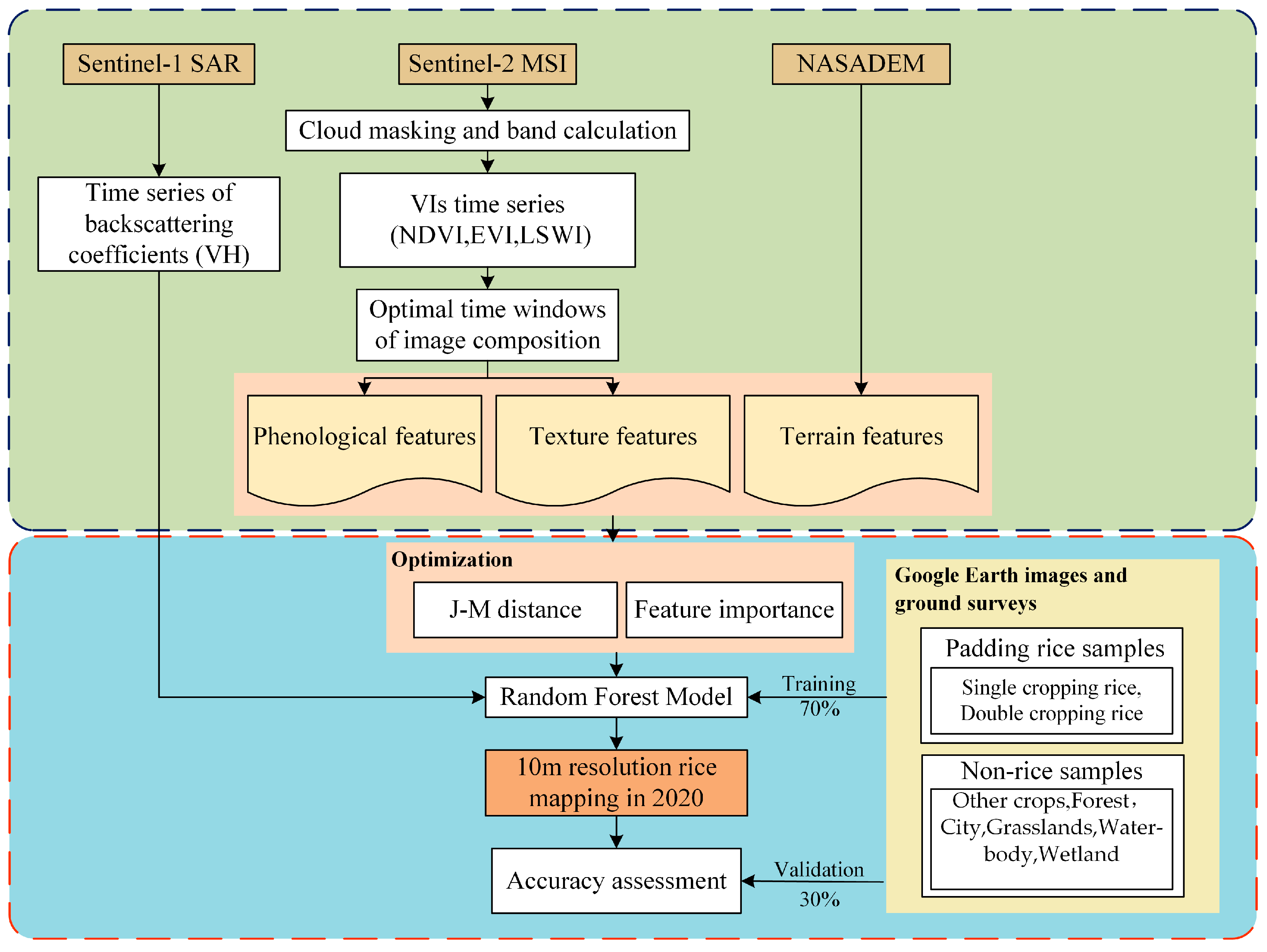
Figure 3 shows the overall workflow of rice mapping, consisting of the following three main steps: (1) identifying three key rice phenological periods by analyzing NDVI, LSWI, and EVI time series profiles; (2) determining the size of the time window for image composition; (3) selecting the optimal way to combine features for different phenological periods; (4) constructing different classification scenarios.

3.1. Padding Rice Phenology Analysis

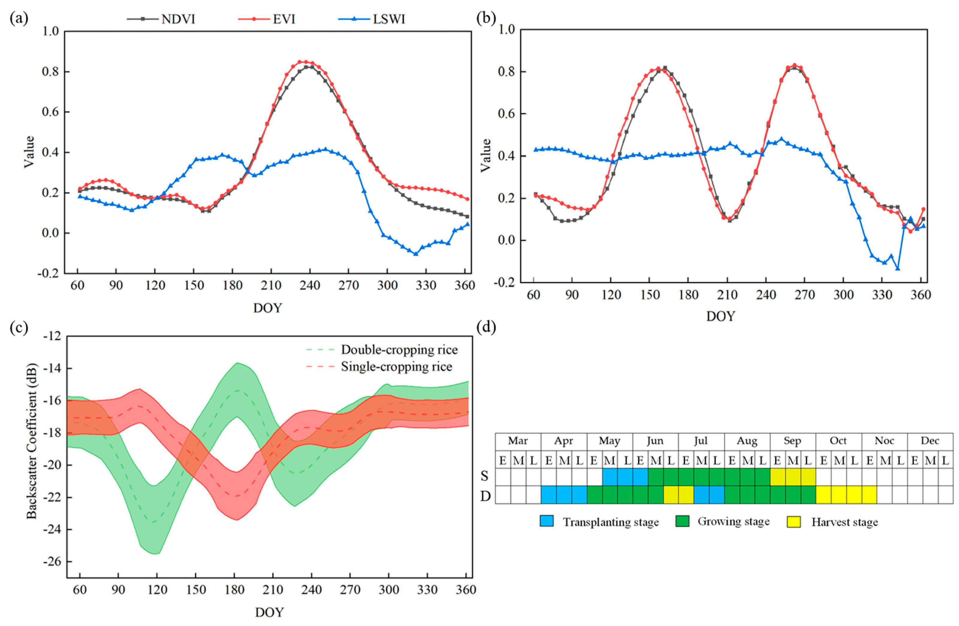
It is essential for paddy rice mapping to identify the characteristics of rice phenology (including transplanting, growing, and harvesting periods). Therefore, in this study, three spectral indices (LSWI, NDVI, and EVI) and VH backscattering coefficient standard time series profiles (Figure 4) were obtained for single- and double-cropping rice to capture their phenological characteristics. More specifically, we used the Google Earth VHR data visual interpretation method and field survey data to select 50 pure rice image pixels each with different cropping intensities, all using the available Sentinel-2 images from March to December 2020 to obtain the three spectral index profiles corresponding to each rice pixel, and averaged all profiles, then passed the Savitzky-Golay (SG) filter to smooth the profiles again. It is worth noting that LSWI is more sensitive to surface soil moisture affected by rain and snow, so we did not smooth the time series of LSWI.

With Figure 4 and Chinese agricultural meteorological data (http://data.cma.cn, accessed on 10 June 2021), three critical stages of rice growth are identified: (1) flooding and transplanting phase—rice was in a mixed soil and water environment during this period, and the flooding and transplanting signals could be identified by using the relationship between EVI, NDVI, and LSWI, where the LSWI value is temporarily greater than the NDVI or EVI value. Meanwhile, the VH backscattering dropped rapidly and reached a peak; (2) growth phase—after transplanting, the rice seedlings started to green up with NDVI and EVI gradually increasing and reaching the maximum value at the peak of growth. The VH backscattering coefficient also showed a significant increasing tendency with increasing plant height and biomass in paddy rice; and (3) harvest phase—when entering the mature harvesting period, EVI and NDVI decreased clearly, while bare soil and post-harvest rice fields exhibited lower LSWI values, which can also be used as a crop harvesting signal [57]. Based on both the spectral and polarization features, we identified three time windows for different types of paddy rice identification (

Table 2. Time windows of image composition for paddy rice mapping.

Paddy Rice Type		Phenology Phases	Time Windows (DOY)
Double cropping paddy rice	Early paddy rice	transplanting phase	90–130
		growth phase	140–180
		harvest phase	180–220
	Late paddy rice	transplanting phase
		growth phase	230–270
		harvest phase	280–320
Single cropping paddy rice	Middle paddy rice	transplanting phase	130–170
		growth phase	195–235
		harvest phase	255–295

). In each key stage, the median values of all valid observations in these time windows were calculated.

3.2. Feature Construction

Feature element selection is an important step in the remote sensing extraction of rice area. Due to the complex cropping structure in the Dongting Lake area, rice cultivation was a mixed system of single- and double-cropping, and there was a large area of wetlands in the lake area, which made it difficult to distinguish the three landscape types: rice, non-rice crops, and wetlands, and it was often difficult to achieve a better recognition effect of rice by using a single-spectral feature, so it was necessary to reasonably add multiple feature variables to effectively improve the rice classification accuracy. In conjunction with the traits of paddy rice and other landscape elements attributes, this paper incorporates phenological features (which include spectral features and the original 12 bands), texture features, and terrain features into the remote sensing classification feature library of the rice-cropping area, based on a machine learning algorithm to enhance the distinction between rice and non-rice categories, as follows:

(1) Spectral features. According to the characteristics of both vegetation and water in rice, a total of seven vegetation indices, including NDVI, EVI, RVI, GCVI, MSAVI, BSI, and PSRI, two water indices, LSWI and MNDWI, and building indices, such as NDBI, are selected, and three common red-edge indices, MTCI, NDRE1 and REP (Red Edge Position Index), were also selected based on the unique red-edge bands of the Sentinel-2 data. The above spectral-index characteristics are shown in

Table 3. Calculation formula for the selected spectral index.

Band Name	Expression	References
NDVI	(NIR − Red)/(NIR + Red)	Carlson et al. [58]
EVI	2.5 × (NIR − Red)/(NIR + 6 × Red − 7.5 × Blue + 1)	Huete et al. [59]
RVI	NIR/Red	Jackson et al. [60]
GCVI	NIR/Green − 1	Ozdoganet al. [61]
MSAVI	(2NIR + 1$-\sqrt{{(2\mathrm{NIR}+1)}^2 - 8(\mathrm{NIR} - \mathrm{Red})}$)/2	Qi et al. [62]
BSI	(SWIR1 + Red) − (NIR + Blue)/(SWIR1 + Red + NIR + Blue)	Nguyen et al. [63]
PSRI	(Red − Blue)/Red Edge2	Merzlyak et al. [64]
LSWI	(NIR − SWIR2)/(NIR + SWIR2)	Xiao et al. [65]
MNDWI	(GREEN − SWIR1)/(GREEN + SWIR1)	Xu et al. [66]
NDBI	(SWIR1 − NIR)/(SWIR1 + NIR)	Zhang et al. [67]
MTCI	(Red Edge2 − Red Edge1)/(Red Edge1 − Red)	Dash et al. [68]
NDRE1	(Red Edge2 − Red Edge1)/(Red Edge2 + Red Edge1)	Giteson et al. [69]
REP	705 + 35 × ((((Red Edge3 + Red)/2) − Red Edge1)/(Red Edge2 − Red Edge1))	Frampton et al. [70]

.

(2) Texture features: as one of the important attributes of an image, reflects the spatial relationship and distribution characteristics of image element gray levels. Gray-level Co-occurrence Martraix (GLCM) is a method that is widely applied in statistical analysis of textures, and describes texture features by studying the spatial-correlation properties of gray levels. GEE provides a speedy computational function based on GLCM texture features called glcmTexture (size, kernel, average), which will be obtained from the grayscale image, Gray, in a line-weighted manner in Equation (1), as the input image of the function, and finally six primary texture features are selected to participate in the classification, which are angular second moment (ASM), contrast (CON), correlation (CORR), variance (VAR), Inverse Difference Moment (IDM) and Entropy (ENT).

$$Gray=0.3B8+0.59B4+0.11B3$$

(1)

where B8, B4 and B3 are the NIR band, Red band and Green band in the sentinel-2 image, respectively.

(3) Terrain features. We calculate terrain-related parameters such as elevation, slope, aspect, and hillshade with the help of the platform’s built-in function ee.Terrain.products(). The median synthesis was executed for rice of different maturation systems according to the time window of each growth stage, and the above spectral, texture, and terrain features were input to the images as separate spectral bands. Finally, we obtained the feature set with rice lifetime attributes.

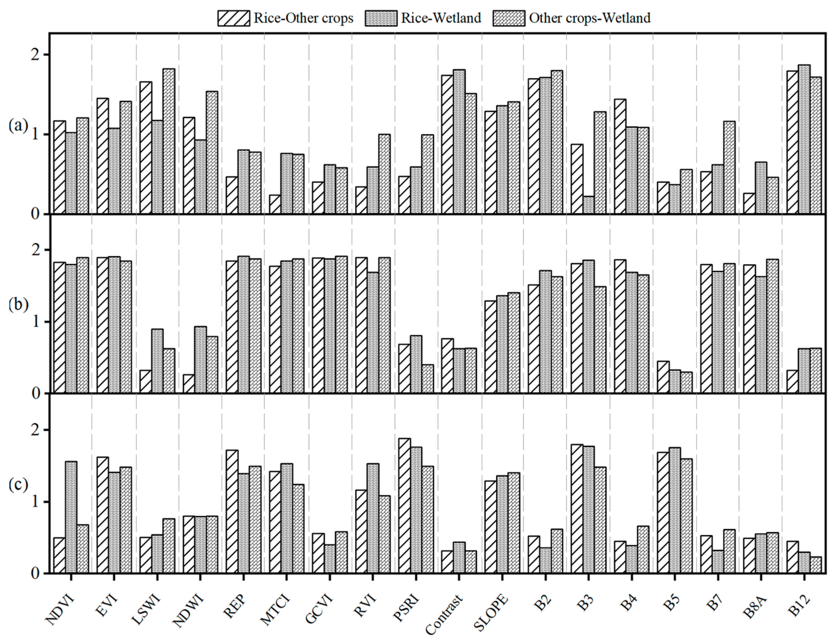
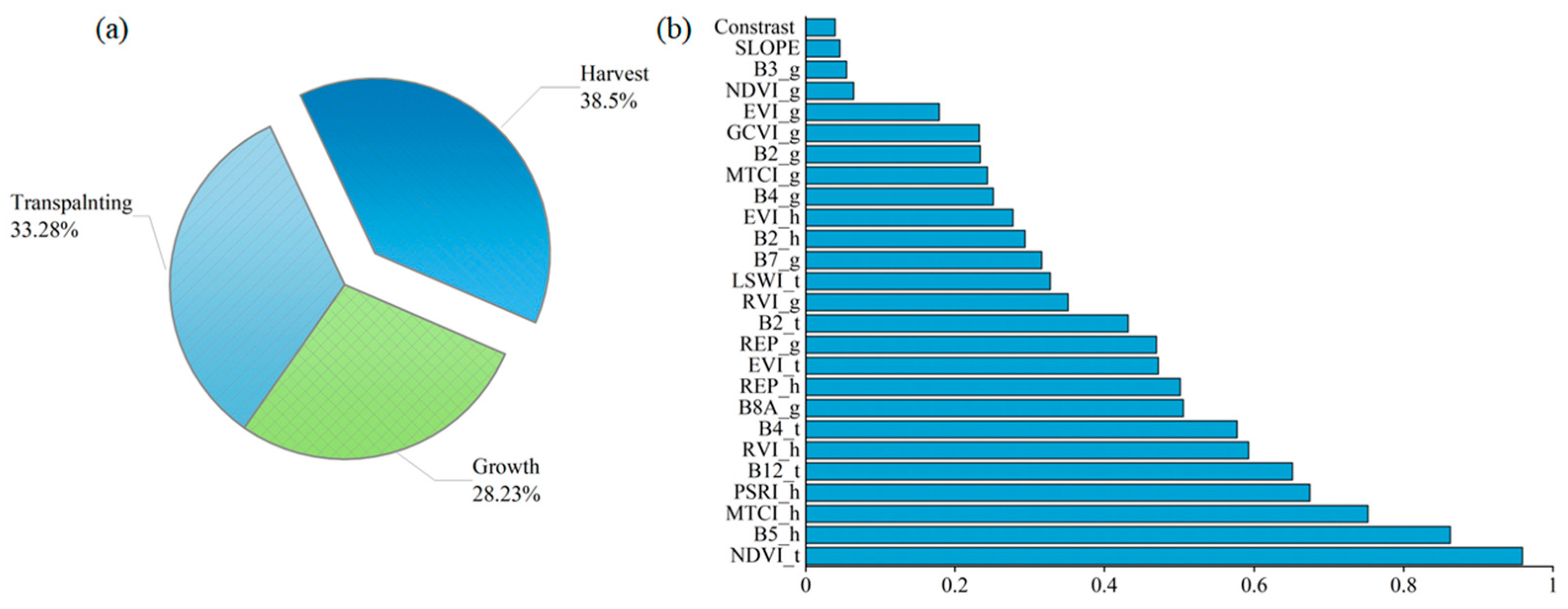
3.3. Feature Optimization and Combination

In this paper, we take advantage of the SEaTH algorithm (Separability and Thresholds) to quantitatively analyze the separability between rice and non-rice at different phenological periods and to determine the optimal combination of characters accordingly. The basic idea of the algorithm is to use the Jeffries–Matusita distance (J m distance) under the condition that the classification features obey a normal distribution. Jeffries–Matusita distance (J m distance) measures interclass differentiability. The formula is below:

$$J=2(1-e^{-B})$$

(2)

$$B=\frac{1}{8}{(m_1-m_2)}^2\times \frac{2}{{\sigma }_1{}^2+{\sigma }_2{}^2}+\frac{1}{2}\ln \left[\frac{{\sigma }_1{}^2+{\sigma }_2{}^2}{2{\sigma }_1{\sigma }_2}\right]$$

(3)

where B denotes the baroclinic distance; and m_i and σ_i, i = 1, 2, represent the mean and variance of a feature of class C1 and class C2, respectively. The interval of J is from 0 to 2, where the larger the value of J, the higher the separability. Considering the transferability of the classification model, we propose to select the features with separation greater than 1 among all three crops. This is mainly based on two points; on the one hand, it further compresses the number of features, and on the other hand, it also shows that the selected features can maximize the separability between categories, which effectively improves the computational efficiency.

3.4. Paddy Rice Extraction Algorithm

In this study, we use a random forest (RF) approach to map rice. Specifically, Sentinel-1/2 time series features and training samples are used to train RF classification models to distinguish rice from others. RF is a machine learning algorithm proposed by Breiman in 2001 [71]. It is a self-learning, integrated machine-learning algorithm based on decision trees, using the bootstrap resampling method to construct decision trees by randomly selecting samples from the training sample set, and combining the prediction results of all decision trees to vote for the final result. The random forest algorithm is a common technical tool for remote sensing mapping of crops because of its fast computing speed, robust model, and strong generalization ability. To balance the prediction accuracy and computation time of the random forest model, the number of Trees was set to 100 in this study, and other parameters were kept as the default settings in GEE.

3.5. Accuracy Assessment

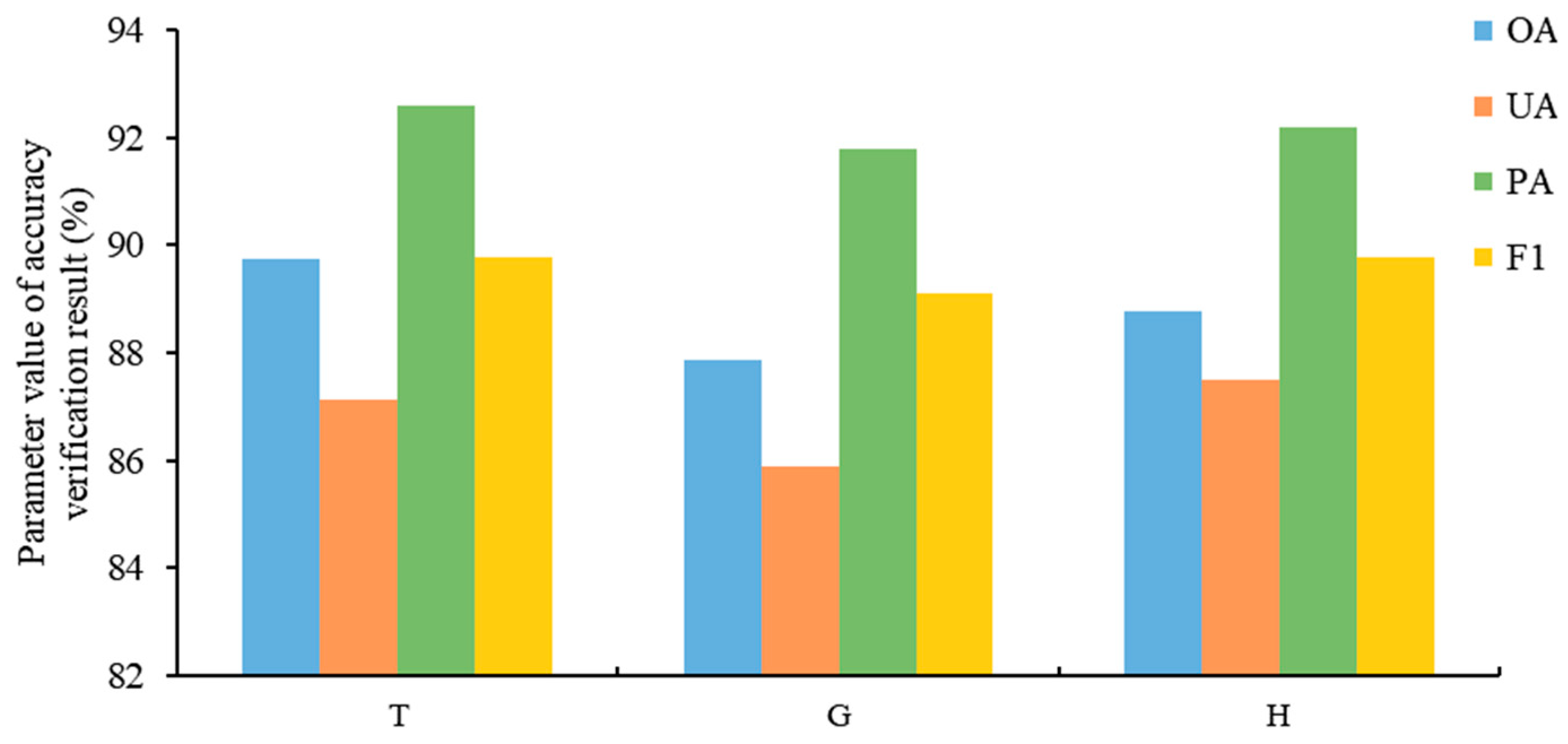
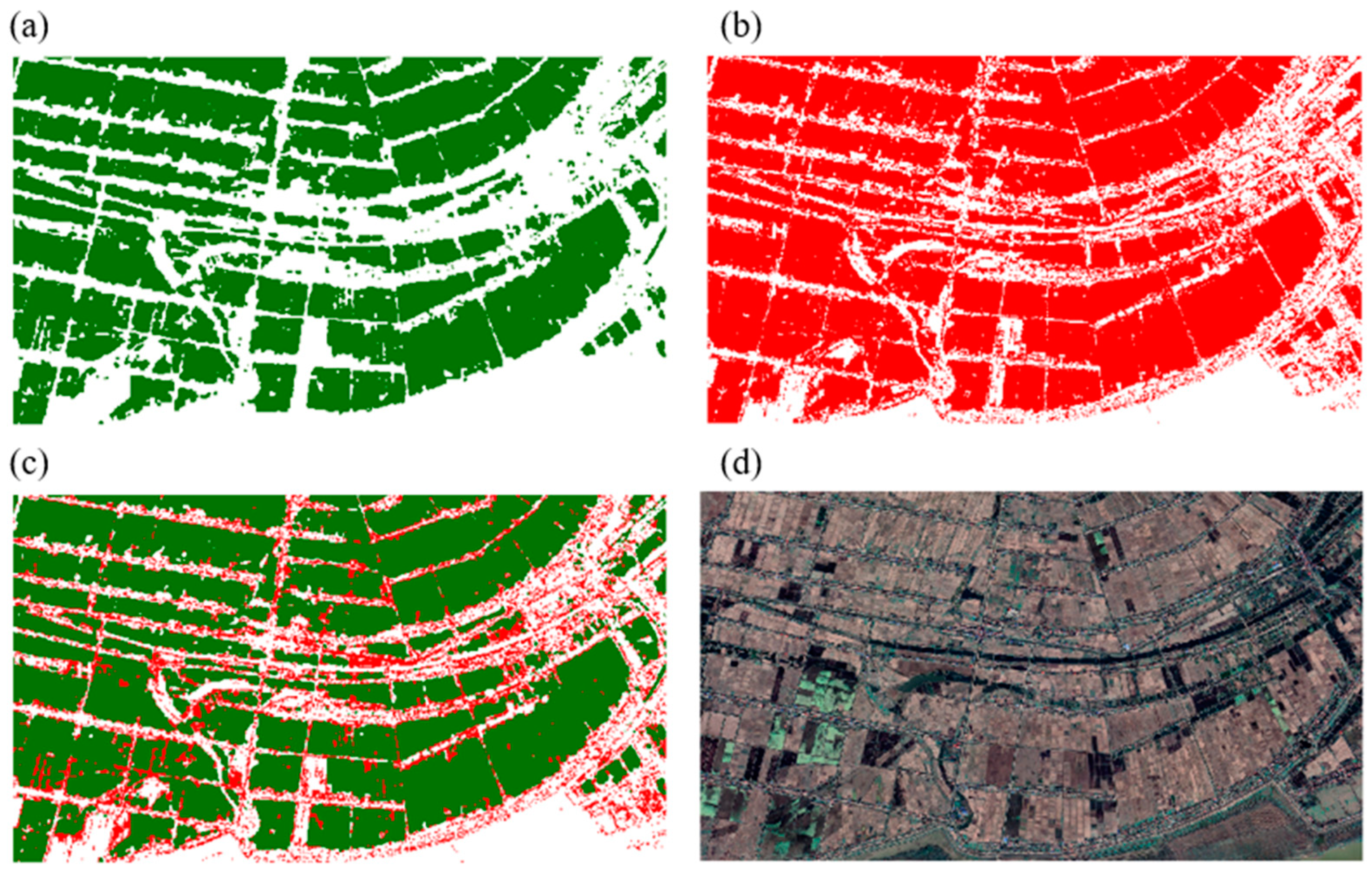
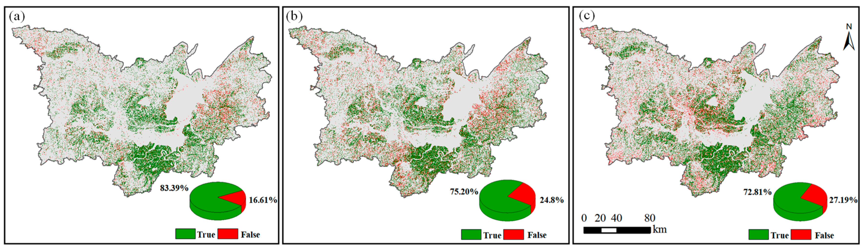
To fully demonstrate the reliability of paddy rice mapping, we have evaluated the classification accuracy and verified the spatial consistency of the rice mapping results. More specifically, we conducted: (1) Five evaluation indexes, including overall accuracy (OA), producer accuracy (PA), user accuracy (UA), and F1 score, which were calculated by establishing a confusion matrix, and thereby quantitatively assessed the accuracy of the mapping results, (2) and compared with the rice visual-interpretation results of Google Earth’s very high-resolution data. 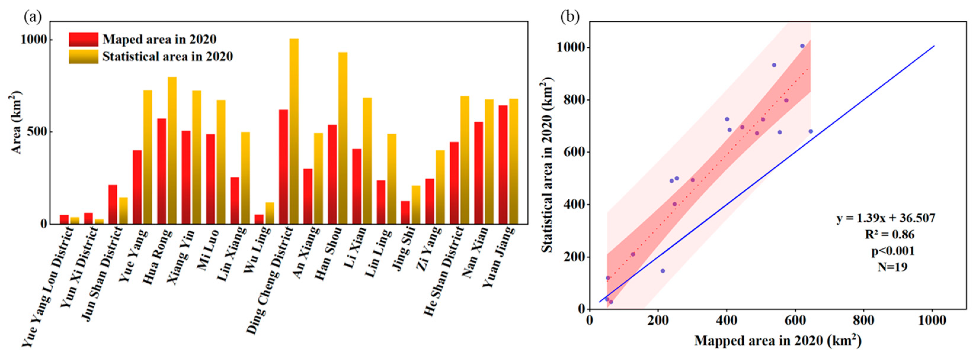(3) Coefficient of determination (R²) and root mean square error (RMSE) were used to evaluate the degree of correlation between the statistical results of rice area (single-cropping rice and double-cropping rice) of 19 counties, and those of the National Bureau of Statistics.

$$OA=\frac{{\displaystyle {\sum }_{i=1}^{\mathrm{n}}{t}_i}}{V}\times 100\%$$

(4)

$$UA=(t_i/m_i)\times 100\%$$

(5)

$$PA=(t_i/v_i)\times 100\%$$

(6)

$$F_i=\frac{2P{A}_i\times U{A}_i}{P{A}_i+U{A}_i}\times 100\%$$

(7)

where n is the total number of classification categories, i is a specific category, V is the total number samples used for verification, t_i represents the number of correctly classified pixels, v_i is the number of type i validation samples, and m_i is the number of validation samples classified as type i.

4. Results

4.1. Spectral Separability

In this study, primitive feature sets (consisting of 12 primitive band features, 13 spectral features, 6 texture features, and 4 topographic features) for different phenological periods were constructed to improve the interclass differentiation among rice, other crops, and wetlands, and the JM distance for screening the best combination of features to meet the differentiability requirements. Figure 5 describes the separability statistics of features between rice and other crops, rice and wetlands, and other crops and wetlands. The first two features with a JM distance greater than one among them, during transplanting, were B12 (1.72–1.87) and LSWI (1.172–1.82), respectively. Owing to the fact that the field is filled with water during transplanting, the surface humidity increases, and both LSWI and B12 bands are sensitive to soil moisture changes. It is worth noting that for rice and other crops, this period is the best time to distinguish them from each other. The highest J m values obtained during the growth period were for two vegetation characteristics, REP and GCVI. In the southern region, the rice growing season is mostly accompanied by the arrival of the rainy season. In particular, for the period from April to mid-September 2020 strong precipitation events were frequent in the area north of central Hunan Province. The distinguishability between rice and wetlands was greatest at this stage, which was attributed to the enhanced surface-water signal in wetlands during this period, while rice showed a strong vegetation greenness signal. In summary, the selected taxonomic characteristics of rice at each stage are shown in

Table 4. The results of JM distance-based feature optimization for each growth stage.

Phenology Stages	Filtered Features	Amount
Transplanting stage	B2, B4, B12, NDVI, EVI, LSWI, Constrast, SLOPE	8
Growing stage	B2, B3, B4, B7, B8A, NDVI, EVI, REP, MTCI, GCVI, RVI, SLOPE	12
Harvest stage	B5, EVI, MTCI, REP, PSRI, RVI, SLOPE	7

.

4.2. Feature Importance Assessment

There are 26 candidate feature factors that are filtered by J m distance, where the significance in rice identification is evaluated based on the variable importance metrics of the random forest itself, and the importance score of each feature in the key phenological period of paddy rice growth is calculated by using the ee.classifier.explain(), as well as ranking the importance of each feature factor in descending order, and adding features one by one to evaluate the overall paddy rice extraction precision to optimize the feature set and reduce data redundancy. From Figure 6, it can be shown that the distinct features differ in their contribution in different stages. Throughout the period of cultivation, the maturity period contributed the most to the classification accuracy of paddy rice, while the growth period provided the least. It was worth noting that both the terrain and texture features could play an appropriate role in the classification to improve the precision, but the role was not obvious. In addition, besides the NDVI_t band with the highest contribution, the importance ranking of the feature factors with red-edge participation is also comparatively advanced, such as B5, MTCI, PSRI, REP, etc., which also implies that the red-edge band plays an important role in rice identification.

According to the optimal dimensional–discrimination method of the selection of feature variables described in the above section, the OA change as the feature variables are added one by one as shown in Figure 7. It is shown that the overall accuracy of paddy rice identification reaches the maximum when the number of features reaches 14, and then the OA decrease slightly and tend to fluctuate in a certain range as the number of feature variables increases. Therefore, the optimal number of subsets of feature factors for model input is 14, which means that the first 14 features in descending order of importance are identified as the final optimized feature combinations.

4.3. Accuracy Assessment of Paddy Rice

4.3.1. Classification Accuracy

We use the validation sample set described in Section 2.2.3 to evaluate the accuracy of the planting intensity map at 10 m spatial resolution in the Dongting Lake area in 2020. The accuracy of the rice extraction results is quantitatively evaluated using the confusion matrix (

Table 5. Confusion matrix of the paddy rice map accuracy assessment.

Validation Samples	Classified Result			Accuracy (%)
	Single	Double	Non-Rice	Producer Accuracy (%)	User Accuracy (%)	F1-Score (%)
Single	509	11	13	94.96	92.38	93.65
Double	9	556	2	97.72	94.88	96.27
Non-rice	33	19	861	94.30	97.73	95.98
Overall accuracy = 95.44%

), and the OA is 95.44%, which meets the requirements for high-precision rice extraction overall. The PA, OA, and F1 scores of both single- and double-cropping rice are above 90%. Meanwhile, the classification accuracy of single-cropping rice is lower than that of double-cropping rice. This lower recognition accuracy of single-cropping rice is mainly due to the fact that the study area is dominated by double-cropping rice; the distribution of single-cropping rice is relatively small and scattered, and the existence of mixed pixels leads to serious misclassification and omission of single-cropping rice extraction.

4.3.2. Analysis of Paddy Rice Distribution Patterns and Spatial Consistency Verification

The distribution of paddy rice in the zone is relatively wide, with double-cropping paddy rice dominating, while the spatial distribution of single- and double-cropping paddy rice is intertwined and mixed (Figure 8). The total area of the paddy rice field covered 6.736 × 10⁷ hm², accounting for 26.10% of the total area in the zone. The rice fields are mainly located in the plains with altitudes less than 50 m and slopes less than 5°. The double-cropping rice is concentrated in Huarong County in the northern part of the lake, Hanshou County in the central part, Dingcheng District in Changde City, Xiangyin County in the South Dongting Lake area, Ziyang District and Heshan District in Yiyang City, and the northwestern part of Yuanjiang City and Miluo City in the East Dongting Lake, while the single-cropping rice has concentrated in small areas in the central part of Li County and the western parts of Huarong County and Nan County. The double-cropping rice pattern is rather large, regular, and continuous, while the single-cropping rice pattern is smaller and more fragmented. Compared with the plain areas, the hilly areas in the mountains are characterized by less arable land, fragmented distribution, and greater difficulty in machine cultivation, and the employment status of half-workers and half-farmers makes most farmers prefer planting single-cropping rice, which accelerates the planting of single-cropping rice in the hilly areas to a wide extent.

Based on the results (Figure 9) of the visual interpretation of four typical sample areas (Figure 8) to verify spatial consistency, it can be qualitatively concluded that the spatial distribution features of rice extracted by this model roughly matches those of the high-resolution image, and the patchy, fragmented water bodies, roads, and shrubs were effectively eliminated.

In addition, we selected three areas for mixed cropping. Each area is a square with a side length of 0.5 km. They were interpreted using ground reference data and polygons with different cropping intensities that were created. We selected the high-resolution Google image data from 3 August 2020, to distinguish between parcels with different cropping systems, because at that time, single-cropping rice cultivation had reached its peak and late rice cultivation of double-cropping rice was at its transplanting stage. These polygons were used to quantitatively evaluate the classification accuracy of rice in different cultivation systems. In Figure 10, we can graphically illustrate the results of the accuracy assessment. In general, small areas not cultivated with rice, small lakes with floating greenery, and shrubs along rivers are more likely to be misclassified as rice pixels, which is mainly due to the resolution size of our images of 10 m, while the landscapes that are smaller than 10 m, as mentioned above, are difficult to subdivide. In summary, our classification results for different rice cropping systems strongly agree with the results of the visual interpretation on the ground.

4.3.3. Analysis of Differences between Rice Mapping in Different Growth Periods

To compare the identifiability of rice at different phenological stages, we classified the composite image data based on the optimal feature set at each stage, and the accuracy verification results are shown in Figure 11. The overall accuracy of paddy rice at each stage was above 85%. The overall accuracy t of the transplanting stage was 89.76%, the highest among the three stages, while the growing stage had the worst detection rate. This indicates that the transplanting stage is the most satisfactory growth stage for rice extraction. We evaluated the spatial distribution variability of rice classification results corresponding to the three main phenological stages based on rice mapping with complete phenological characteristics. Figure 12 shows the differences in rice extraction effects at different growth stages, where the green labels are correct image pixels, i.e., the basemap matches the rice classification results at this stage, and the red labels are misclassified and omitted pixels in rice classification at this stage. The spatial distribution of the red and green areas in the figure shows that there is little difference between the rice extraction results of the three key stages and the basemap, and that the results of rice mapping are consistent in the plain of the lake, while the red areas are mainly found in the hilly areas. Considering the percentage of correct identification rate of rice pixels, we can see that the rice detection result of transplantation stages has the least difference with the basemap, and the correct identification rate of rice pixels is 83.39%. The least agreement of rice recognition results was in the maturity phase, where the rice recognition error rate reached 21.79%.

4.3.4. Comparison with the National Statistical Data

We compared the rice cultivation map with agricultural statistics in 2020 using 19 county-level administrative districts in the Dongting Lake area as the statistical unit (Figure 13). At the same time, we conducted correlation analysis and significance analysis and concluded that there is a significant linear relationship between rice mapping products and statistical data, with a coefficient of determination R² of 0.86, and a significant correlation at the level of p < 0.001. Meanwhile, the RMSE were 217.5 km². It is worth noting that most of the paddy rice cropping fields extracted, based on the county-level model, was smaller than the statistical sown area with a relative error of 32.85%. The reasons for this situation were mainly the difficulties in implementing large-scale mechanized planting in areas with complicated terrain, the existence of many abandoned paddy fields and conversion of paddy fields, and the inconsistency between the data on paddy fields reported by farmers and the actual data on cultivated areas in the current year.

5. Discussion

5.1. Evaluation of the Reliability of Multiple Feature Selection in Rice Identification

It has been successfully demonstrated that the method of obtaining phenological characteristics for rice identification is feasible by analyzing the temporal dynamics of spectral indices. For example, the LSWI and NDFI indices, which are sensitive to soil inundation, and the NDVI and EVI indices, which are more sensitive to changes in vegetation chlorophyll and biomass, have been widely used to monitor key stages of rice cultivation and have effectively mapped rice growing areas in different geographical regions. Zhu et al. [72] analyzed the profiles of EVI and LSWI time series and the relationship between them to identify the phenological characteristics for mapping rice in different cropping systems in southern China. However, the above indices could not capture the whole lifetime signature of rice. To solve this problem, Dong et al. [73] integrated six spectral indices (BSI, LSWI, GCVI, NDVI, EVI, and PSRI) for four different phenological periods for the first time to achieve seasonal biophysical characterization of rice cultivation throughout its life cycle. However, there are limitations in the richness and adaptability of the classification features that need to be improved.

Due to the considerable regional differences between the north and south, and the variability of phenological information on rice, as well as the spatial heterogeneity of rice distribution in the south, which is scattered, highly fragmented, and has a more complicated planting structure, existing rice identification methods applicable to apartment areas may not be able to perform the high-precision extraction of rice in complex terrain. In our work, in addition to the six indicators mentioned above, we also consider topography, texture, and some indices about the red edge of vegetation to detect the growth of rice at each stage to achieve precise identification of rice fields. Based on the spectral separability statistics, feature importance evaluation, and accuracy evaluation of the classification results at each stage, we found that except for the commonly visible bands (B2, B4), which had a high separation for rice, wetlands, and other plants during transplanting, SWIR 2 bands also achieved better separation and contributed more to classification accuracy. This was attributed to the fact that SWIR2 is sensitive to water retention in leaves and has lower reflectance during transplanting, so the flooding signal in rice fields was more pronounced in the SWIR 2 band [74,75]. In addition, the indices involved in the red-edge band greatly varies seasonally with the index characteristics of the water body, and the red-edge characteristics are closely related to the state of vegetation growth, which can improve the saturation phenomenon caused by the absence of red-edge indices (e.g., NDVI, EVI) during dense vegetation growth [76]. Figure 4 and Table 4 also show that the red-edge index was mainly used for rice at the growth and maturity stages, mainly to distinguish rice from other plants. The results of the identification of rice at each stage show that the filtered and optimized feature set can fully perform the function of complete attributes of the whole life span of paddy rice. To further evaluate the need for the selected multiple features, a combination of NDVI time series and VH polarization image data were used as input features to the random forest classifier to obtain classification results based on a single feature (

Table 6. Confusion matrix of rice maps using temporal single spectral features.

Validation Samples	Classified Result			Accuracy (%)
	Single	Double	Non-Rice	Producer Accuracy (%)	User Accuracy (%)	F1-Score (%)
Single	463	25	36	88.36	86.06	8719
Double	28	513	11	92.93	92.60	92.91
Non-rice	47	16	874	93.28	94.90	94.08
Overall accuracy = 91.90%

). When compared with our maps, based on the very high-resolution imagery, the single spectral feature of temporal NDVI identified most pixels with cropland, but wetlands, some non-rice crops, and shrubs and grasses near roads were easily misclassified as rice, leading to an overestimation of the extent of rice cultivation, while the “salt and pepper” effect on classification was severe (Figure 14).

5.2. The Advantages of Rice Identification Method Based on Optical and SAR Image Fusion

Frequent rainfall in the southern region of China limits the availability of high-quality optical imagery, thus limiting the number of available time windows for classification features. The low use of optical image data in the growing season results in features in the growing season contributing less to rice identification. The exclusive use of optical data for classification without cloud-polluted time windows may weaken classification accuracy to some extent, while microwave data do not have the limitation of missing images due to cloud effects. Therefore, data from SAR can be used to supplement optical data to improve the temporal frequency of high-quality observations. Combining optical and SAR imagery can capture different aspects of rice phenological characteristics. Integrating images from different sensors combines the advantages of both data sources and effectively avoids the shortcomings of a single data source, on the one hand, and increases the accuracy of the algorithm’s computational results to some extent, on the other. Using three different sensor combinations for rice identification, we found that the accuracy of rice identification with integrated Sentinel-1 and Sentinel-2 images is higher than with Sentinel-1 or Sentinel-2 alone (

Table 7. Classification accuracy of rice types under three different scenarios.

Scheme	Overall Accuracy (%)	Crop Types	Producer Accuracy (%)	User Accuracy (%)	F1-Score (%)
S1	87.98%	Double	91%	94.45%	92.69
		Single	87.91	78.95%	83.19
S2	91.41%	Double	95.06%	96.39%	95.72
		Single	90.94%	83.27%	86.94
S1 + S2	93.80%	Double	97.72%	94.88%	96.28
		Single	94.96%	92.24%	93.65

). The classification efficiency of the optical images from Sentinel-2 is better than that of the images from SAR.

5.3. Uncertainty of the Algorithm

Although a pixel-based composite method of phenological features was used to extract the distribution of rice cultivation with high accuracy, there are still some limitations. There are mixed pixels at the intersection of rice and other landscape classes that can be easily overlooked or misclassified. Extreme rainfall may also cause the surface water level of non-rice crops to rise during rice transplanting and flooding, resulting in other crops that have similar growth stages to rice being easily mistaken for rice, especially single-cropping rice.

The object-based image classification algorithm, which analyzes objects by integrating neighborhood information, has been shown to be advantageous in identifying fragmented rice paddies compared to traditional pixel-based classification methods [77]. The algorithm uses the spectral, spatial, and textural information of the landscape to collect a set of homogeneous objects that do not overlap, reducing the “salt and pepper” effect in heterogeneous landscapes [36]. These unsupervised extracted objects do not take into account the combination of multidimensional feature information, such as image morphological information and contextual semantic information, and often, the obtained object units do not match the morphology of the actual target features.

In recent years, Deep Learning has made great progress in image classification research [78]. It can actively learn and evaluate the typical features of features embedded in huge remote sensing images in a data-driven manner, which offers the possibility of highly accurate remote sensing of the spatial distribution of crops. Using GEE for cloud computing and analyzing large-scale remote sensing data in conjunction with deep learning frameworks (e.g., TensorFlow, etc.), and developing deep learning classification algorithms with stronger autonomous learning capability is an important way to improve the accuracy of large-scale rice extraction models and their generalization capability.

6. Conclusions

Based on the Google Earth Engine cloud platform, we combined Sentinel-1/2 time series imagery with a prior knowledge of the spectral and polarization properties of seasonal rice growth, proposed a pixel-based mapping algorithm for rice phenology, and generated an annual map of rice fields with 10 m spatial resolution in the Dongting Lake area in 2020. The main results are as follows:

(1)

Based on the evaluation of the separation between different features under different phenological stages and the importance of classification features, we found that throughout the rice growing season, the classification features at maturity contributed most to the classification accuracy of rice, and while the contribution of the growing period was the least, spectral features played a dominant role in classification, while texture and topographic features had the least influence with feature factors involving red margins playing an important role at each phenological stage of rice recognition.

(2)

The accuracy of the rice map using the complete phenological features is better than that of individual phenological stages, whereas the identification rate of rice at the transplanting stage is the highest compared to the growth stage and maturity stage, with a correct rate of 83.39%, in which the difference of rice identification results is smaller in the plain area of the lake, while the identification rate is worse for rice in the hilly area with complex terrain.

(3)

We found that the rice classification accuracy using fused Sentinel-1 and Sentinel-2 images was higher than that of either Sentinel-1 or Sentinel-2 alone, with the former achieving an overall accuracy of 93.8%, while F1 scores for both single- and double-cropping rice were above 93%. This study demonstrates that Sentinel-1/2 images are useful for cloudy and fragmented southern China areas for monitoring rice distribution and intensity.

This research provides highly accurate and effective rice (single- and double-cropping rice) map information in the Dongting Lake area, which can be a supplementary information source for ground survey data to save a lot of human and material resources. Meanwhile, we hope that the rice map can effectively guide governmental decision-makers to reasonably regulate rice types and timely participate in area dynamics to enhance rice production in the face of frequent extreme weather times.

References

1. Seck, P.A.; Diagne, A.; Mohanty, S.; Wopereis, M. Crops that feed the world 7: Rice. Food Secur. 2012, 4, 7–24. [Google Scholar] [CrossRef]
2. He, Y.; Dong, J.; Liao, X.; Sun, L.; Wang, Z.; You, N.; Li, Z.; Fu, P. Examining rice distribution and cropping intensity in a mixed single-and double-cropping region in South China using all available Sentinel 1/2 images. Int. J. Appl. Earth Obs. Geoinf. 2021, 101, 102351. [Google Scholar] [CrossRef]
3. Shang, Q.; Yang, X.; Gao, C.; Wu, P.; Liu, J.; Xu, Y.; Shen, Q.; Zou, J.; Guo, S. Net annual global warming potential and greenhouse gas intensity in Chinese double rice-cropping systems: A 3-year field measurement in long-term fertilizer experiments. Glob. Chang. Biol. 2011, 17, 2196–2210. [Google Scholar] [CrossRef]
4. Ito, A.; Tohjima, Y.; Saito, T.; Umezawa, T.; Hajima, T.; Hirata, R.; Saito, M.; Terao, Y. Methane budget of East Asia, 1990–2015: A bottom-up evaluation. Sci. Total Environ. 2019, 676, 40–52. [Google Scholar] [CrossRef]
5. Silalertruksa, T.; Gheewala, S.H.; Mungkung, R.; Nilsalab, P.; Lecksiwilai, N.; Sawaengsak, W. Implications of water use and water scarcity footprint for sustainable rice cultivation. Sustainability 2017, 9, 2283. [Google Scholar] [CrossRef]
6. Bouman, B.A.; Humphreys, E.; Tuong, T.P.; Barker, R. Rice and water. Adv. Agron. 2007, 92, 187–237. [Google Scholar]
7. Menenti, M.; Li, X.; Jia, L.; Yang, K.; Pellicciotti, F.; Mancini, M.; Shi, J.; Escorihuela, M.J.; Zheng, C.; Chen, Q. Multi-Source Hydrological Data Products to Monitor High Asian River Basins and Regional Water Security. Remote Sens. 2021, 13, 5122. [Google Scholar] [CrossRef]
8. Bhadha, J.; Khatiwada, R.; Galindo, S.; Xu, N.; Capasso, J. Evidence of soil health benefits of flooded rice compared to fallow practice. Sustain. Agric. Res. 2018, 7, 31–41. [Google Scholar] [CrossRef]
9. Saurabh, K.; Rao, K.; Mishra, J.; Kumar, R.; Poonia, S.; Samal, S.; Roy, H.; Dubey, A.; Choubey, A.K.; Mondal, S. Influence of tillage based crop establishment and residue management practices on soil quality indices and yield sustainability in rice-wheat cropping system of eastern Indo-Gangetic Plains. Soil Tillage Res. 2021, 206, 104841. [Google Scholar] [CrossRef]
10. Maltchik, L.; Stenert, C.; Batzer, D.P. Can rice field management practices contribute to the conservation of species from natural wetlands? Lessons from Brazil. Basic Appl. Ecol. 2017, 18, 50–56. [Google Scholar] [CrossRef]
11. Heino, M.; Puma, M.J.; Ward, P.J.; Gerten, D.; Heck, V.; Siebert, S.; Kummu, M. Two-thirds of global cropland area impacted by climate oscillations. Nat. Commun. 2018, 9, 1257. [Google Scholar] [CrossRef] [PubMed]
12. Tan, M.; Li, X.; Xie, H.; Lu, C. Urban land expansion and arable land loss in China—A case study of Beijing–Tianjin–Hebei region. Land Use Policy 2005, 22, 187–196. [Google Scholar] [CrossRef]
13. Döös, B.R. Population growth and loss of arable land. Glob. Environ. Chang. 2002, 12, 303–311. [Google Scholar] [CrossRef]
14. Prasad, R.; Shivay, Y.S.; Kumar, D. Current status, challenges, and opportunities in rice production. In Rice Production Worldwide; Springer: Cham, Switzerland, 2017; pp. 1–32. [Google Scholar]
15. Tang, Z.; Deng, G.; Hu, G.; Zhang, H.; Pan, H.; Sang, G. Satellite observed spatiotemporal variability of snow cover and snow phenology over high mountain Asia from 2002 to 2021. J. Hydrol. 2022, 613, 128438. [Google Scholar] [CrossRef]
16. Dong, J.; Xiao, X. Evolution of regional to global paddy rice mapping methods: A review. ISPRS J. Photogramm. Remote Sens. 2016, 119, 214–227. [Google Scholar] [CrossRef]
17. Xiao, X.; Boles, S.; Frolking, S.; Li, C.; Babu, J.Y.; Salas, W.; Moore, B., III. Mapping paddy rice agriculture in South and Southeast Asia using multi-temporal MODIS images. Remote Sens. Environ. 2006, 100, 95–113. [Google Scholar] [CrossRef]
18. Zhang, G.; Xiao, X.; Dong, J.; Kou, W.; Jin, C.; Qin, Y.; Zhou, Y.; Wang, J.; Menarguez, M.A.; Biradar, C. Mapping paddy rice planting areas through time series analysis of MODIS land surface temperature and vegetation index data. ISPRS J. Photogramm. Remote Sens. 2015, 106, 157–171. [Google Scholar] [CrossRef]
19. Liu, L.; Xiao, X.; Qin, Y.; Wang, J.; Xu, X.; Hu, Y.; Qiao, Z. Mapping cropping intensity in China using time series Landsat and Sentinel-2 images and Google Earth Engine. Remote Sens. Environ. 2020, 239, 111624. [Google Scholar] [CrossRef]
20. Rad, A.M.; Ashourloo, D.; Shahrabi, H.S.; Nematollahi, H. Developing an automatic phenology-based algorithm for rice detection using sentinel-2 time-series data. IEEE J. Sel. Top. Appl. Earth Obs. Remote Sens. 2019, 12, 1471–1481. [Google Scholar]
21. Pan, Z.; Huang, J.; Zhou, Q.; Wang, L.; Cheng, Y.; Zhang, H.; Blackburn, G.A.; Yan, J.; Liu, J. Mapping crop phenology using NDVI time-series derived from HJ-1 A/B data. Int. J. Appl. Earth Obs. Geoinf. 2015, 34, 188–197. [Google Scholar] [CrossRef]
22. Pan, L.; Xia, H.; Yang, J.; Niu, W.; Wang, R.; Song, H.; Guo, Y.; Qin, Y. Mapping cropping intensity in Huaihe basin using phenology algorithm, all Sentinel-2 and Landsat images in Google Earth Engine. Int. J. Appl. Earth Obs. Geoinf. 2021, 102, 102376. [Google Scholar] [CrossRef]
23. Defourny, P.; Bontemps, S.; Bellemans, N.; Cara, C.; Dedieu, G.; Guzzonato, E.; Hagolle, O.; Inglada, J.; Nicola, L.; Rabaute, T. Near real-time agriculture monitoring at national scale at parcel resolution: Performance assessment of the Sen2-Agri automated system in various cropping systems around the world. Remote Sens. Environ. 2019, 221, 551–568. [Google Scholar] [CrossRef]
24. Deng, G.; Tang, Z.; Hu, G.; Wang, J.; Sang, G.; Li, J. Spatiotemporal dynamics of snowline altitude and their responses to climate change in the Tienshan Mountains, Central Asia, During 2001–2019. Sustainability 2021, 13, 3992. [Google Scholar] [CrossRef]
25. Tang, Z.; Wang, X.; Deng, G.; Wang, X.; Jiang, Z.; Sang, G. Spatiotemporal variation of snowline altitude at the end of melting season across High Mountain Asia, using MODIS snow cover product. Adv. Space Res. 2020, 66, 2629–2645. [Google Scholar] [CrossRef]
26. Qiu, B.; Lu, D.; Tang, Z.; Chen, C.; Zou, F. Automatic and adaptive paddy rice mapping using Landsat images: Case study in Songnen Plain in Northeast China. Sci. Total Environ. 2017, 598, 581–592. [Google Scholar] [CrossRef]
27. Schlund, M.; Erasmi, S. Sentinel-1 time series data for monitoring the phenology of winter wheat. Remote Sens. Environ. 2020, 246, 111814. [Google Scholar] [CrossRef]
28. Wang, Y.; Fang, S.; Zhao, L.; Huang, X.; Jiang, X. Parcel-based summer maize mapping and phenology estimation combined using Sentinel-2 and time series Sentinel-1 data. Int. J. Appl. Earth Obs. Geoinf. 2022, 108, 102720. [Google Scholar] [CrossRef]
29. Carrasco, L.; O’Neil, A.W.; Morton, R.D.; Rowland, C.S. Evaluating combinations of temporally aggregated Sentinel-1, Sentinel-2 and Landsat 8 for land cover mapping with Google Earth Engine. Remote Sens. 2019, 11, 288. [Google Scholar] [CrossRef]
30. Karimi, N.; Taban, M.R. A convex variational method for super resolution of SAR image with speckle noise. Signal Process. Image Commun. 2021, 90, 116061. [Google Scholar] [CrossRef]
31. Singha, M.; Dong, J.; Zhang, G.; Xiao, X. High resolution paddy rice maps in cloud-prone Bangladesh and Northeast India using Sentinel-1 data. Sci. Data 2019, 6, 26. [Google Scholar] [CrossRef]
32. Yang, H.; Pan, B.; Wu, W.; Tai, J. Field-based rice classification in Wuhua county through integration of multi-temporal Sentinel-1A and Landsat-8 OLI data. Int. J. Appl. Earth Obs. Geoinf. 2018, 69, 226–236. [Google Scholar] [CrossRef]
33. Yang, H.; Pan, B.; Li, N.; Wang, W.; Zhang, J.; Zhang, X. A systematic method for spatio-temporal phenology estimation of paddy rice using time series Sentinel-1 images. Remote Sens. Environ. 2021, 259, 112394. [Google Scholar] [CrossRef]
34. You, N.; Dong, J. Examining earliest identifiable timing of crops using all available Sentinel 1/2 imagery and Google Earth Engine. ISPRS J. Photogramm. Remote Sens. 2020, 161, 109–123. [Google Scholar] [CrossRef]
35. Fiorillo, E.; Di Giuseppe, E.; Fontanelli, G.; Maselli, F. Lowland Rice Mapping in Sédhiou Region (Senegal) Using Sentinel 1 and Sentinel 2 Data and Random Forest. Remote Sens. 2020, 12, 3403. [Google Scholar] [CrossRef]
36. Cai, Y.; Lin, H.; Zhang, M. Mapping paddy rice by the object-based random forest method using time series Sentinel-1/Sentinel-2 data. Adv. Space Res. 2019, 64, 2233–2244. [Google Scholar] [CrossRef]
37. Van Tricht, K.; Gobin, A.; Gilliams, S.; Piccard, I. Synergistic use of radar Sentinel-1 and optical Sentinel-2 imagery for crop mapping: A case study for Belgium. Remote Sens. 2018, 10, 1642. [Google Scholar] [CrossRef]
38. Veloso, A.; Mermoz, S.; Bouvet, A.; Le Toan, T.; Planells, M.; Dejoux, J.-F.; Ceschia, E. Understanding the temporal behavior of crops using Sentinel-1 and Sentinel-2-like data for agricultural applications. Remote Sens. Environ. 2017, 199, 415–426. [Google Scholar] [CrossRef]
39. Soh, N.C.; Shah, R.M.; Giap, S.G.E.; Setiawan, B.I.; Minasny, B. High-Resolution Mapping of Paddy Rice Extent and Growth Stages across Peninsular Malaysia Using a Fusion of Sentinel-1 and 2 Time Series Data in Google Earth Engine. Remote Sens. 2022, 14, 1875. [Google Scholar]
40. Löw, F.; Michel, U.; Dech, S.; Conrad, C. Impact of feature selection on the accuracy and spatial uncertainty of per-field crop classification using support vector machines. ISPRS J. Photogramm. Remote Sens. 2013, 85, 102–119. [Google Scholar] [CrossRef]
41. Peña-Barragán, J.M.; Ngugi, M.K.; Plant, R.E.; Six, J. Object-based crop identification using multiple vegetation indices, textural features and crop phenology. Remote Sens. Environ. 2011, 115, 1301–1316. [Google Scholar] [CrossRef]
42. Dong, J.; Xiao, X.; Kou, W.; Qin, Y.; Zhang, G.; Li, L.; Jin, C.; Zhou, Y.; Wang, J.; Biradar, C. Tracking the dynamics of paddy rice planting area in 1986–2010 through time series Landsat images and phenology-based algorithms. Remote Sens. Environ. 2015, 160, 99–113. [Google Scholar] [CrossRef]
43. Gorelick, N.; Hancher, M.; Dixon, M.; Ilyushchenko, S.; Thau, D.; Moore, R. Google Earth Engine: Planetary-scale geospatial analysis for everyone. Remote Sens. Environ. 2017, 202, 18–27. [Google Scholar] [CrossRef]
44. Pekel, J.-F.; Cottam, A.; Gorelick, N.; Belward, A.S. High-resolution mapping of global surface water and its long-term changes. Nature 2016, 540, 418–422. [Google Scholar] [CrossRef] [PubMed]
45. Li, K.; Xu, E. High-accuracy continuous mapping of surface water dynamics using automatic update of training samples and temporal consistency modification based on Google Earth Engine: A case study from Huizhou, China. ISPRS J. Photogramm. Remote Sens. 2021, 179, 66–80. [Google Scholar] [CrossRef]
46. Liang, J.; Xie, Y.; Sha, Z.; Zhou, A. Modeling urban growth sustainability in the cloud by augmenting Google Earth Engine (GEE). Comput. Environ. Urban Syst. 2020, 84, 101542. [Google Scholar] [CrossRef]
47. Liu, X.; Hu, G.; Chen, Y.; Li, X.; Xu, X.; Li, S.; Pei, F.; Wang, S. High-resolution multi-temporal mapping of global urban land using Landsat images based on the Google Earth Engine Platform. Remote Sens. Environ. 2018, 209, 227–239. [Google Scholar] [CrossRef]
48. Gong, P.; Li, X.; Zhang, W. 40-Year (1978–2017) human settlement changes in China reflected by impervious surfaces from satellite remote sensing. Sci. Bull. 2019, 64, 756–763. [Google Scholar] [CrossRef]
49. Chen, B.; Xiao, X.; Li, X.; Pan, L.; Doughty, R.; Ma, J.; Dong, J.; Qin, Y.; Zhao, B.; Wu, Z. A mangrove forest map of China in 2015: Analysis of time series Landsat 7/8 and Sentinel-1A imagery in Google Earth Engine cloud computing platform. ISPRS J. Photogramm. Remote Sens. 2017, 131, 104–120. [Google Scholar] [CrossRef]
50. Koskinen, J.; Leinonen, U.; Vollrath, A.; Ortmann, A.; Lindquist, E.; d’Annunzio, R.; Pekkarinen, A.; Käyhkö, N. Participatory mapping of forest plantations with Open Foris and Google Earth Engine. ISPRS J. Photogramm. Remote Sens. 2019, 148, 63–74. [Google Scholar] [CrossRef]
51. Wang, X.; Xiao, X.; Zou, Z.; Hou, L.; Qin, Y.; Dong, J.; Doughty, R.B.; Chen, B.; Zhang, X.; Chen, Y. Mapping coastal wetlands of China using time series Landsat images in 2018 and Google Earth Engine. ISPRS J. Photogramm. Remote Sens. 2020, 163, 312–326. [Google Scholar] [CrossRef]
52. Zhang, Z.; Xu, N.; Li, Y.; Li, Y. Sub-continental-scale mapping of tidal wetland composition for East Asia: A novel algorithm integrating satellite tide-level and phenological features. Remote Sens. Environ. 2022, 269, 112799. [Google Scholar] [CrossRef]
53. Phalke, A.R.; Özdoğan, M.; Thenkabail, P.S.; Erickson, T.; Gorelick, N.; Yadav, K.; Congalton, R.G. Mapping croplands of Europe, Middle East, Russia, and Central Asia using Landsat, Random Forest, and Google Earth Engine. ISPRS J. Photogramm. Remote Sens. 2020, 167, 104–122. [Google Scholar] [CrossRef]
54. Lobell, D.B.; Thau, D.; Seifert, C.; Engle, E.; Little, B. A scalable satellite-based crop yield mapper. Remote Sens. Environ. 2015, 164, 324–333. [Google Scholar] [CrossRef]
55. Jin, Z.; Azzari, G.; You, C.; Di Tommaso, S.; Aston, S.; Burke, M.; Lobell, D.B. Smallholder maize area and yield mapping at national scales with Google Earth Engine. Remote Sens. Environ. 2019, 228, 115–128. [Google Scholar] [CrossRef]
56. Son, N.-T.; Chen, C.-F.; Chen, C.-R.; Toscano, P.; Cheng, Y.-S.; Guo, H.-Y.; Syu, C.-H. A phenological object-based approach for rice crop classification using time-series Sentinel-1 Synthetic Aperture Radar (SAR) data in Taiwan. Int. J. Remote Sens. 2021, 42, 2722–2739. [Google Scholar] [CrossRef]
57. Chen, Y.; Lu, D.; Moran, E.; Batistella, M.; Dutra, L.V.; Sanches, I.D.A.; da Silva, R.F.B.; Huang, J.; Luiz, A.J.B.; de Oliveira, M.A.F. Mapping croplands, cropping patterns, and crop types using MODIS time-series data. Int. J. Appl. Earth Obs. Geoinf. 2018, 69, 133–147. [Google Scholar] [CrossRef]
58. Carlson, T.N.; Ripley, D.A. On the relation between NDVI, fractional vegetation cover, and leaf area index. Remote Sens. Environ. 1997, 62, 241–252. [Google Scholar] [CrossRef]
59. Huete, A.; Didan, K.; Miura, T.; Rodriguez, E.P.; Gao, X.; Ferreira, L.G. Overview of the radiometric and biophysical performance of the MODIS vegetation indices. Remote Sens. Environ. 2002, 83, 195–213. [Google Scholar] [CrossRef]
60. Jackson, R.D.; Huete, A.R. Interpreting vegetation indices. Prev. Vet. Med. 1991, 11, 185–200. [Google Scholar] [CrossRef]
61. Ozdogan, M.; Gutman, G. A new methodology to map irrigated areas using multi-temporal MODIS and ancillary data: An application example in the continental US. Remote Sens. Environ. 2008, 112, 3520–3537. [Google Scholar] [CrossRef]
62. Qi, J.; Chehbouni, A.; Huete, A.R.; Kerr, Y.H.; Sorooshian, S. A modified soil adjusted vegetation index. Remote Sens. Environ. 1994, 48, 119–126. [Google Scholar] [CrossRef]
63. Nguyen, C.T.; Chidthaisong, A.; Kieu Diem, P.; Huo, L.-Z. A modified bare soil index to identify bare land features during agricultural fallow-period in southeast Asia using Landsat 8. Land 2021, 10, 231. [Google Scholar] [CrossRef]
64. Merzlyak, M.N.; Gitelson, A.A.; Chivkunova, O.B.; Rakitin, V.Y. Non-destructive optical detection of pigment changes during leaf senescence and fruit ripening. Physiol. Plant. 1999, 106, 135–141. [Google Scholar] [CrossRef]
65. Xiao, X.; Boles, S.; Liu, J.; Zhuang, D.; Frolking, S.; Li, C.; Salas, W.; Moore III, B. Mapping paddy rice agriculture in southern China using multi-temporal MODIS images. Remote Sens. Environ. 2005, 95, 480–492. [Google Scholar] [CrossRef]
66. Xu, H. Modification of normalised difference water index (NDWI) to enhance open water features in remotely sensed imagery. Int. J. Remote Sens. 2006, 27, 3025–3033. [Google Scholar] [CrossRef]
67. Zhang, Y.; Odeh, I.O.; Han, C. Bi-temporal characterization of land surface temperature in relation to impervious surface area, NDVI and NDBI, using a sub-pixel image analysis. Int. J. Appl. Earth Obs. Geoinf. 2009, 11, 256–264. [Google Scholar] [CrossRef]
68. Dash, J.; Curran, P. The MERIS terrestrial chlorophyll index. Int. J. Remote Sens. 2004, 25, 5403–5413. [Google Scholar] [CrossRef]
69. Gitelson, A.A.; Gritz, Y.; Merzlyak, M.N. Relationships between leaf chlorophyll content and spectral reflectance and algorithms for non-destructive chlorophyll assessment in higher plant leaves. J. Plant Physiol. 2003, 160, 271–282. [Google Scholar] [CrossRef]
70. Frampton, W.J.; Dash, J.; Watmough, G.; Milton, E.J. Evaluating the capabilities of Sentinel-2 for quantitative estimation of biophysical variables in vegetation. ISPRS J. Photogramm. Remote Sens. 2013, 82, 83–92. [Google Scholar] [CrossRef]
71. Breiman, L. Random forests. Mach. Learn. 2001, 45, 5–32. [Google Scholar] [CrossRef]
72. Zhu, L.; Liu, X.; Wu, L.; Liu, M.; Lin, Y.; Meng, Y.; Ye, L.; Zhang, Q.; Li, Y. Detection of paddy rice cropping systems in southern China with time series Landsat images and phenology-based algorithms. GIScience Remote Sens. 2021, 58, 733–755. [Google Scholar] [CrossRef]
73. Ni, R.; Tian, J.; Li, X.; Yin, D.; Li, J.; Gong, H.; Zhang, J.; Zhu, L.; Wu, D. An enhanced pixel-based phenological feature for accurate paddy rice mapping with Sentinel-2 imagery in Google Earth Engine. ISPRS J. Photogramm. Remote Sens. 2021, 178, 282–296. [Google Scholar] [CrossRef]
74. Xia, L.; Zhao, F.; Chen, J.; Yu, L.; Lu, M.; Yu, Q.; Liang, S.; Fan, L.; Sun, X.; Wu, S. A full resolution deep learning network for paddy rice mapping using Landsat data. ISPRS J. Photogramm. Remote Sens. 2022, 194, 91–107. [Google Scholar] [CrossRef]
75. Yi, Z.; Jia, L.; Chen, Q. Crop classification using multi-temporal Sentinel-2 data in the Shiyang River Basin of China. Remote Sens. 2020, 12, 4052. [Google Scholar] [CrossRef]
76. Guo, Y.; Ren, H. Remote sensing monitoring of maize and paddy rice planting area using GF-6 WFV red edge features. Remote Sens. 2023, 207, 107714. [Google Scholar] [CrossRef]
77. Zhao, R.; Li, Y.; Ma, M. Mapping paddy rice with satellite remote sensing: A review. Sustainability 2021, 13, 503. [Google Scholar] [CrossRef]
78. LeCun, Y.; Bengio, Y.; Hinton, G. Deep learning. Nature 2015, 521, 436–444. [Google Scholar] [CrossRef]
Figure 1. (a) Location of Dongting Lake Area in Hunan Province, China, (b) Digital Elevation Model (DEM), and (c) Slope distribution map of Dongting Lake area.
Remotesensing 15 02794 g001
Figure 2. Spatial distribution of Sentinel-1/2 valid observation numbers in Dongting Lake area during rice growing season. (a) Sentinel-1 data, (b) Sentinel-2 data.
Remotesensing 15 02794 g002
Figure 3. Mapping paddy rice workflow overview.
Remotesensing 15 02794 g003
Figure 4. (a,b) Spectral-temporal feature curves profiles over different crop types; (c) The time series curves of backscattering coefficient for VH for double cropping rice, single cropping rice; (d) Rice cropping phenological calendar of Hunan province, where S stands for single-cropping rice and D stands for double-cropping rice.
Remotesensing 15 02794 g004
Figure 5. J m statistics of different crop types at different phenological periods under spectral indices. (ac) represent the transplanting, growing, and harvesting periods, respectively.
Remotesensing 15 02794 g005
Figure 6. (a) Percentage importance of features at different growth stages (b) Normalized importance sorting of crop classification features, where NDVI_t represents the NDVI value at the transplanting period, and similarly NDVI_g and NDVI_h represent the NDVI values at the growing and maturing periods, respectively.
Remotesensing 15 02794 g006
Figure 7. Relationship between rice recognition accuracy and the number of spectral features.
Remotesensing 15 02794 g007
Figure 8. Spatial distribution extraction results of rice in Dongting Lake area in 2020. Four selected validation regions are denoted as a, b, c, and d.
Remotesensing 15 02794 g008
Figure 9. Comparison between our maps and visual interpretation results. (ad), respectively, represent Google Earth VHR data (eh) show the composite reference image (bands: SWIR1/SWIR2/NIR). (il) paddy rice map of visual interpretation from Google Earth image. (mp) show our rice mapping result at a spatial resolution of 10 m.
Remotesensing 15 02794 g009
Figure 10. (a1c1) Google Earth image (a2c2) Reference data by visual interpretation based on Google Earth image. (a3c3) rice cropping intensity results of this paper.
Remotesensing 15 02794 g010
Figure 11. Accuracy of classification of each growth stage for paddy rice. T, G, H stand for the transplanting period, the growing period and the harvest period, respectively.
Remotesensing 15 02794 g011
Figure 12. Spatial distribution difference map of rice classification results between three growth stages of rice and the base map, (ac) stand for the transplanting period, the growing period and the harvest period, respectively.
Remotesensing 15 02794 g012
Figure 13. (a) Comparison of sown area estimates by county between the 2020 cropping intensity map and the 2020 reported agricultural statistics. (b) The blue line is the y = x line, and the red area is the 95% confidence interval and predicted area.
Remotesensing 15 02794 g013
Figure 14. Our maps are compared with rice mapping results based on time-series NDVI spectral features; where (a,b) are the rice results from this study and the rice mapping results based on a single spectral feature, respectively; (c) are the overlay of the two results to highlight the differences; (d) are high-resolution Google Earth image data.
Remotesensing 15 02794 g014