1. Introduction
Research has shown that climate change creates warmer temperatures and drier conditions, leading to longer wildfire seasons and increased wildfire risks in many areas in the United States [
1,
2]. These factors have, in turn, led to increases in the frequency, extent, and severity of wildfires [
3,
4]. According to the National Centers for Environmental Information (NCEI) [
5], which keeps track of weather and climate events with significant economic impacts, there have been 20 wildfire events exceeding USD 1 billion in damages in the United States from 1980 to 2022 (adjusted for inflation), and 16 of those have occurred since 2000 [
3]. In the western United States, climate change has doubled the forest fire area from 1984 to 2015 [
6].
Given the danger posed by wildland fires to people, property, wildlife, and the environment, there is an urgent need to provide tools for effective wildfire management. Currently, wildfires are detected by humans trained to be on the lookout for wildfires, residents in an area, or passersby. A more reliable approach is needed for early wildfire detection, which is essential to minimizing potentially catastrophic destruction. In this work, we describe a deep learning model for automated wildfire smoke detection to provide early notification of wildfires.
In previous work [
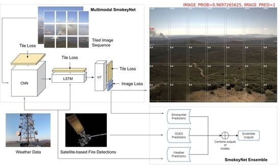
7], we introduced FIgLib (Fire Ignition Library), a dataset of labeled wildfire smoke images from fixed-view cameras; and SmokeyNet, a novel deep learning architecture using spatiotemporal information from optical camera image sequences to detect smoke from wildland fires. Here, we extend that work by investigating the efficacy of adding additional data sources to our camera-based smoke detection system—specifically, satellite-based fire detections and weather sensor measurements. Satellite-based fire detections may detect fires that are hidden from the cameras behind hills or other occluders. Weather factors such as humidity can affect how a wildfire grows and changes. Adding these additional inputs thus provides additional data that can further inform SmokeyNet, potentially leading to better smoke detection performance in terms of both accuracy and detection time. As the three data sources have different temporal and spatial resolutions, integrating all three requires several nontrivial data processing steps, as well as complex architectural changes to our deep learning model.
We make the following contributions for multimodal wildland fire smoke detection: (1) data processing techniques for integrating the different types of data with different spatial and temporal scales; (2) SmokeyNet Ensemble, an ensemble approach to integrate multiple data sources; (3) Multimodal SmokeyNet, an extension of SmokeyNet to incorporate additional data types; and (4) a comparative analysis of multimodal approaches to the baseline SmokeyNet in terms of accuracy metrics as well as time-to-detect, which is important for the early detection of wildfires.
2. Related Work
Recently, deep learning approaches have employed a combination of convolutional neural networks (CNNs) [
8,
9], background subtraction [
10,
11], and object detection methods [
12,
13] to incorporate visual and spatial features. Long short-term memory (LSTM) networks [
10,
12] and optical flow [
14,
15] methods have been applied to incorporate temporal context from video sequences.
Due to the lack of a benchmark dataset to evaluate model performance, the high accuracies reported in many papers on the detection of smoke from images may not be representative of real-world performance across different scenarios. For instance, Ko [
16] and Jeong [
12] use video sequences either with or without a fire, but none with a fire starting in the middle of a sequence. Li [
17] and Park [
8] use image inputs wherein smoke plumes are more visible compared to video frames where the smoke is initially forming after ignition. Yin [
18] uses images representing smoke in scenarios beyond wildland fires. In other works, such as Park [
8], Zhang [
19], and Yuan [
20], images are synthetically generated to overcome the lack of available data.
Govil et al. [
21] is the only work we are aware of that also uses the FIgLib dataset to evaluate wildfire smoke detection performance, using an InceptionV3 CNN trained from scratch as the primary image classification architecture. The authors reported a test accuracy of 0.91 and an F1-score of 0.89. However, the test set consists of only a small number of hand-selected images relative to the training set (250 vs. 8500+ images). The test set also contains images from the same video sequences of fires used in the training set, with only 10 min (i.e., 10 frames) of separation between them; this procedure bleeds information from the training data, and therefore may overstate the performance on the test set.
Peng and Wang [
22] combined hand-designed smoke features with an optimized SqueezeNet network for smoke detection. A smoke detection rate of 97.74% was reported. However, they used the relatively small dataset created by Lin et al. [
23], which consists of 15 HD videos (10 smoke and 5 nonsmoke). Khan et al. [
9] used an EfficientNet CNN architecture for smoke detection and DeepLabv3+ semantic segmentation architecture for smoke localization. Model performance was reported on both image inputs as well as video sequences. However, this model was trained for indoor and outdoor scenarios and not for wildfires. Hence, while the model was tested on custom-collected wildfire data, quantitative results for these data were not reported by the authors. Mukhiddinov et al. [
24] also curated a custom wildfire image dataset that was used to train a YOLOv5m model for wildfire smoke detection, reporting an average precision of 79.3% on the test set.
There has been some work carried out using weather data for detection of wildfires. Da Penha and Nakamura [
25] make use of wireless sensor networks (WSNs) to collect temperature and light intensity data from the surroundings to detect wildfires using information fusion methods. They propose a threshold-based algorithm and a Dempster–Shafer method for forest fire detection, and claim that the former is more reliable. Díaz-Ramírez et al. [
26] expand on this idea to include humidity data as well. However, such methods require the sensors to be installed very close to the fire. Moreover, the experiments they conducted are from a small time frame of 10 days, which is not sufficient to understand the efficacy of their algorithm in different seasons.
In our previous work [
7], we presented the SmokeyNet deep learning model that detects smoke from wildland fires using images from optical cameras. The model consists of a CNN [
27], LSTM [
28], and a vision transformer [
29]. Here, we use SmokeyNet as a baseline, and extend it with additional weather data and satellite-based fire detections to investigate the effects of these additional data sources on performance in terms of accuracy and detection time.
Our main focus is on detecting wildfires from camera images as soon as possible after ignition for early notification. In most scenarios, smoke will be spotted before the actual fire can be seen. In addition, the field of view of the camera may be blocked by terrain, making it difficult to spot the actual fire from the camera. Therefore, detecting smoke is a faster way to indicate the presence of a wildland fire than trying to detect the fire itself. It is also worth noting that the detection of fires, rather than smoke, is a different research problem that requires different approaches (e.g., infrared vs optical cameras), and is a rich but separate field with numerous research efforts, and hence, we are not currently considering fire detection in our work.
3. Data
The work presented in this paper makes use of data from three different sources: images from optical cameras, weather sensor measurements, and fire detections from satellite data. Camera data from the FIgLib library provide images with and without smoke; our SmokeyNet model was originally trained on these camera images. Weather factors such as temperature and relative humidity play a role in the likelihood of wildfire ignition. Combined with wind conditions, these can affect how a wildfire grows and changes, and consequently, the appearance of smoke. Additionally, weather can also affect the appearance of clouds, which can cause false positives in our model. These considerations are the motivation for adding weather data to the model. The integration of fire detections from satellite data was motivated by the potential for such detections to identify wildfires missed by SmokeyNet. For instance, fires could be occluded by hills or mountains from optical cameras on the ground, so satellite-based systems might detect fires before ground camera-based systems. Thus, we wanted to investigate if adding satellite-based fire detections and weather data to the baseline SmokeyNet would help to improve the overall performance of the model. This section describes the FIgLib data, weather data, and satellite fire detection data in detail.
3.1. FIgLib Data
The baseline dataset used in our work is the Fire Ignition images Library (FIgLib) dataset. FIgLib consists of sequences of wildland fire images captured at one-minute intervals from fixed-view optical cameras located throughout southern California, which are part of the High Performance Wireless Research and Education Network (HPWREN) [
30]. The dataset contains nearly 20,000 images, and covers multiple terrains, including mountainous, desert, and coastal areas, and also contains sequences from throughout the year, thus capturing seasonal variations. Each sequence consists of images from before and after initial fire ignition. To the best of our knowledge, FIgLib is the largest publicly available labeled dataset for training smoke detection models.
Each image is 1536 × 2048 or 2048 × 3072 pixels in size, depending on the camera model used. Each FIgLib sequence has been curated to contain images before and after the start of a wildfire that can be used for training and evaluating machine learning models. Typically, each sequence consists of images from 40 min prior to and 40 min following fire ignition, for a total of 81 images, with a balance between positive and negative images.
To avoid out-of-distribution sequences, the FIgLib dataset was filtered to remove fire sequences with black and white images, night fires, and fires with questionable labels, as detailed in [
7]. Additionally, 15 fires without matching weather data were also removed. The resulting FIgLib dataset used in this paper consists of 255 FIgLib fire sequences from 101 cameras across 30 weather stations occurring between 3 June 2016 and 12 July 2021, totaling 19,995 images.
Each image was resized to an empirically determined size of
pixels to speed up training. Further, the top 352 rows of the image, which depict the sky far above the horizon, were cropped. This had the added advantage of removing clouds from the topmost part of the image, reducing false positives that may arise due to the clouds. This resulted in images of size
pixels, which enabled us to evenly divide the image into 45 tiles of size
pixels, overlapping by 20 pixels, to allow for independent processing of each tile. Refer to
Section 4.1 for more details. Data augmentation using horizontal flip; vertical crop; blur; and jitter of color, brightness, and contrast was applied to each image. Each augmentation operation is applied with a 50% probability, and the amount of augmentation is chosen randomly within a specified range. The image pixels were normalized to 0.5 mean and 0.5 standard deviation, as expected by the deep learning library that we used (torchvision). Data augmentation is a standard approach in deep learning to help the model generalize better and prevent overfitting. This entire process of image resizing, cropping, and applying data augmentations was performed as part of the model training pipeline.
The 255 FIgLib fire sequences were partitioned into 131 fires for training, 63 fires for validation, and 61 fires for testing. Fires for training, validation, and testing are mutually exclusive. The number of fires and images in the train, validation, and test partitions are summarized in
Table 1.
3.2. Weather Data
For each FIgLib image, we also extracted the weather data associated with that image. This was accomplished by obtaining sensor measurements from the three weather stations nearest to the camera location and in the direction that the camera is facing. Note that we need the weather corresponding to the scene captured by the camera, not the weather corresponding to the camera location, which may be different. Weather data in the HPWREN [
30,
31], SDG&E [
32], and Southern California Edison (SCE) [
33] networks were fetched from weather stations using the Synoptic’s Mesonet API [
34]. Synoptic is a partner of SDG&E that offers services for storing and serving weather data.
The weather data has 23 attributes, out of which we selected the ones with under 5% missing data: air temperature, relative humidity, wind speed, wind gust, wind direction, dew point temperature. Wind speed and wind direction can be thought of as being the radius and angle in a polar coordinate system, which were then used to obtain Cartesian co-ordinates “u” and “v”. Wind speed and wind direction were thus converted to ’u’ and ’v’ so that aggregation across the three closest weather stations could be performed easily. The wind direction was also adjusted to be relative to the direction that the camera is facing and converted to the corresponding sine and cosine components. Due to the sparsity of many of the weather attributes, some features that may affect the likelihood of ignition, such as soil moisture, were not included in our data. The resulting weather vector consists of the following seven features: air temperature, dew point temperature, relative humidity, wind speed, wind gust, and sine and cosine of wind direction.
Since weather varies from region to region, weather measurements are normalized per station to ensure that relative values are used instead of raw values. Weather measurements are also normalized over an entire year to retain seasonal fluctuations. Normalized weather measurements from the three stations corresponding to each image are then aggregated using a weighted average based on the inverse of the distance between the camera and the weather station. Additionally, since there is a weather data point available every ten minutes, whereas the images are spaced one minute apart, we employed linear interpolation to resolve the difference in temporal resolution. The detailed procedure for obtaining and processing the weather data is explained in
Appendix A.1.
3.3. Satellite Fire Detection Data
In addition to FIgLib camera data and weather data, we also used fire detection data based on satellite images from the Geostationary Operational Environment Satellite (GOES) system. GOES is operated by the National Oceanic and Atmospheric Administration (NOAA) [
35] to support weather monitoring, forecasting, severe storm tracking, and meteorology research [
36,
37]. GOES provides real-time satellite data covering Southern California that are publicly available. Satellite image data from the GOES-R series Advanced Baseline Imager (ABI) are processed by the Wildfire Automated Biomass Burning Algorithm (WFABBA) [
38] in order to detect and characterize fire from biomass burning. The output of WFABBA provides the fire detection data used in our model, as discussed in
Section 4.2.
WFABBA is a rule-based algorithm for dynamic multispectral thresholding to locate and characterize hot spot pixels in a satellite image [
39]. It uses data from the GOES satellites to detect thermal anomalies (i.e., areas of increased temperature) associated with wildfires. These anomalies are identified using a combination of brightness temperature thresholds, temporal and spatial filtering, and statistical analyses. The algorithm also takes into account the presence of clouds and other factors that can affect the accuracy of the detection. Once a thermal anomaly is detected, the WFABBA algorithm generates a fire location and intensity estimate, which is used to produce fire detection maps and other products that can aid in wildfire management and response efforts.
For our work, data from the GOES-16 and GOES-17 satellites were used, where GOES-16 covers North and South America and the Atlantic Ocean to the west coast of Africa while GOES-17 covers western North America and the Pacific Ocean [
37]. The data processed via WFABBA can be accessed at the following link:
https://wifire-data.sdsc.edu/dataset/goes-fire-detections, accessed on 15 March 2023.
We used the metadata generated by the WFABBA system in our experiments. These are text files generated after WFABBA processing of GOES imagery that list the details of the algorithm used, the latitude–longitude of the detected fire (if any), fire size, fire temperature, and other parameters calculated by the algorithm. WFABBA metadata files were parsed, consolidating all data in a single dataframe. We used the latitude–longitude information to match GOES detections with FIgLib, as described in later sections.
Since the spatial and temporal resolutions of FIgLib images were different from those of GOES, we came up with the following procedure for matching FIgLib with GOES data. For every camera associated with FIgLib input images, we selected GOES detections that were within a 35-mile radius of the camera and in its field of view. From this subset, if a detection was found that was within a 20 min window of the FIgLib input, then it was considered a match and was joined with the FIgLib input with a positive prediction value (indicating that fire was detected by WFABBA). If there was no match, a negative prediction value was assigned. This process was carried out for data from both GOES-16 and GOES-17. The 35-mile radius and the 20 min window were determined empirically. A detailed description of the algorithm can be found in Appendices
Appendix A.2 and
Appendix A.3. In the rest of this work, we refer to these data as “GOES data.”
4. Methods
The following three model architectures were used in our experiments:
SmokeyNet: Baseline model that takes an image and its previous frame from a FIgLib fire sequence and predicts smoke/no smoke for the image.
SmokeyNet Ensemble: An ensemble model combining the baseline SmokeyNet model, GOES-based fire predictions, and weather data.
Multimodal SmokeyNet: An extension of the SmokeyNet architecture that incorporates weather data directly into the network.
4.1. SmokeyNet
The baseline SmokeyNet model [
7], depicted in
Figure 2, is a spatiotemporal model consisting of three different networks: a convolutional neural network (CNN) [
27], a long short-term memory model (LSTM) [
28], and a vision transformer (ViT) [
29]. The input to SmokeyNet is a tiled wildfire image and its previous frame from a wildfire image sequence to account for temporal context. A pretrained CNN, namely ResNet34 [
40], extracts feature embeddings from each raw image tile for the two frames independently. These embeddings are passed through an LSTM, which assigns temporal context to each tile by combining the temporal information from the current and previous frame. These temporally combined tiles are passed through a ViT, which encodes spatial context over the tiles to generate the image prediction. The outputs of the ViT are spatiotemporal tile embeddings, and a classification (CLS) token that encapsulates the complete image information [
29]. This token is passed through a sequence of linear layers and a sigmoid activation to generate a single image prediction for the current image.
4.2. SmokeyNet Ensemble
To incorporate GOES predictions, weather data, and FIgLib camera images, we used an ensemble approach to combine SmokeyNet outputs with separate models that we built for the GOES and weather data, as shown in
Figure 3. The SmokeyNet Ensemble model consists of three components: output probabilities obtained from baseline SmokeyNet, GOES-based predictions obtained from the matching algorithm described in
Section 3.3, and outputs of a 32-unit LSTM model used to model time-series weather data to predict the probability of a fire. The input to the model is weather data from the previous 20 min. Both the GOES and weather models are weak models that are used to supplement the stronger SmokeyNet signals in order to improve the accuracy of SmokeyNet.
In order to combine the outputs, we first experimented with a simple voting strategy, such that the class that was output by at least two of the three models became the final output. Using the baseline model accuracies as weights, a weighted average of the predictions from the three models was computed to derive the final prediction. The output class was derived from the averaged probability by using a threshold-based decision rule. In addition, as a separate experiment, we passed the signal vector from the three models through a logistic regressor with the aim of learning the weights used for combining the models. More details on the ensemble setup are provided in
Section 5.2.
4.3. Multimodal SmokeyNet
We also investigated an approach to integrate weather data directly into the SmokeyNet model. This allows for both raw data sources—optical camera images and weather sensor measurements—to be integrated as input to the model. This approach is Multimodal SmokeyNet, and its architecture is depicted in
Figure 4. The input to the model is a series of
images, with each image represented using
tiles, similar to baseline SmokeyNet. For each FIgLib image series passed through the model, the corresponding weather vector, of length
, is incorporated in the model at two places as weather tensors that are concatenated to the CNN and the LSTM embeddings (represented in
Figure 4 as “Normalized Weather Data”). The input weather vector is replicated, via the hidden layer, along the feature dimension, to prevent the CNN/LSTM embeddings from dominating the weather features. The replication is controlled by the replication factor
. The resultant weather tensor output from the hidden layer is such that it matches the dimensions of the respective embedding, and has a length of [
] along the feature dimension. This weather embedding is concatenated with the CNN/LSTM embedding (of size
e). The concatenated embedding is then passed through three hidden layers before tile loss computation, and is also propagated forward to the next component of Multimodal SmokeyNet, as shown in
Figure 4. This is carried out similarly with the weights from the LSTM output to the ViT. Finally, when the output of the hidden layer is sent through the vision transformer, the final model outputs are tile and image probabilities, similar to the baseline SmokeyNet model.
Table 2 lists the dimension parameters shown in
Figure 4. The values for these parameters were determined using hyperparameter tuning, as discussed in
Section 5.3.
The training procedure for the model happens in two stages. First, the baseline SmokeyNet model is trained for 25 epochs on just FIgLib camera images. Using transfer learning, the multimodal model (
Figure 4) is initialized with weights from the trained baseline SmokeyNet model. The concatenation of the weather embeddings to the CNN/LSTM embeddings increases the dimensions of the weights from the CNN output to the LSTM and the weights from the LSTM output to the ViT. These extra connections are initialized with random weights. The multimodal SmokeyNet is then trained with both FIgLib images and weather data, as described in more detail in
Section 5.
Similar to the baseline SmokeyNet, the binary cross-entropy (BCE) training loss for Multimodal SmokeyNet consists of the image loss from the ViT, as well as the tile loss from each of the model’s components: CNN, LSTM, and ViT, as shown in
Figure 2 and described in detail in [
7]. If
I is the total number of tiles, the overall training loss can be summarized as:
5. Experiments and Results
As mentioned in
Section 3.1, we used a train/validation/test split of 131/63/61 fires (or 10,302/4894/4799 images) for all our experiments. Using these datasets, we first ran experiments on the SmokeyNet model to establish a baseline. This baseline model was then used in the SmokeyNet Ensemble and used to initialize the Multimodal SmokeyNet model, as described in this section.
5.1. Baseline SmokeyNet
For the baseline model, we took the original trained SmokeyNet model from [
7] and trained it for an additional 25 epochs. This was to match the additional training that the multimodal SmokeyNet model undergoes so that we had a fair comparison between these two models. The model with the lowest validation loss was selected as the baseline SmokeyNet, used in both SmokeyNet Ensemble and Multimodal SmokeyNet experiments described below.
5.2. SmokeyNet Ensemble Results
The SmokeyNet ensemble combines input from four separate models: SmokeyNet, GOES-16, GOES-17, and weather-based LSTM. The weather-based LSTM, as described in
Section 4.2, was trained in order to capture time-series trends in the weather data. The model was trained using the same training split as SmokeyNet, while the validation set was used to select the best model based on validation accuracy, and also to tune the learning rate. Baseline SmokeyNet is as described in
Section 5.1. Moreover, since both the GOES baseline models were found to be extremely weak predictors, we combined predictions from the GOES-16 and GOES-17 models by performing a logical OR operation (denoted “(GOES-16 || GOES-17)”).
For the ensemble, we started with a simple majority vote strategy, such that the final prediction was the mode of predictions from the three models: SmokeyNet, (GOES-16 || GOES-17), and Weather. Next, since the three models have varying baseline performances, a weighted average of the three predictions was computed using the baseline model validation accuracies as weights. The output class was decided based on a threshold determined by F1 on the validation data. Finally, instead of manually providing weights to the three model predictions, we passed the data through a logistic regression model to have the model learn the weights. The inputs to the model were the binary prediction values from the GOES models and output probabilities obtained from SmokeyNet and the Weather model. These features were used to train a logistic regression model. We also experimented with ridge regression to further evaluate the behavior of the individual base models in terms of contribution to the final ensemble prediction. To find the optimal value of regularization strength (e.g., ) for the ridge regression model, we used grid search on the validation set. All the regression models were trained using the train split used for baseline SmokeyNet.
Table 3 reports the performance of the SmokeyNet Ensemble methods described in
Section 4.2 on the test set. Note that the TTD metric is not reported for these experiments. Due to the difference in temporal resolution of FIgLib data vs. GOES fire detections, the algorithm used to match SmokeyNet predictions with GOES predictions used a sliding window around the timestamp associated with a given FIgLib image, as described in
Section 3.3. The sliding window can contain GOES predictions before or after the timestamp of the FIgLib image, thus making the TTD metric unsuitable for these experiments.
The scores in
Table 3 indicate that weighting the predictions from individual models slightly increases F1 over baseline SmokeyNet (setup 8), though baseline SmokeyNet provides the highest Accuracy and Recall over any ensemble model. Baseline GOES-16 gives the highest Precision (setup 2), although this is due to the very small number of matches between FIgLib and GOES data. As described in
Section 3.3, a GOES detection is considered only if it matches a FIgLib image using the spatial and temporal filters we have defined. The small number of matches for GOES-16 thus results in a very high Precision and correspondingly very low Recall.
For the experiments using logistic regression (setups 9, 10, 11), the results are very close to those of baseline SmokeyNet, indicating that the model could be learning to assign the highest weight to the SmokeyNet output probability that was passed as a feature. This hypothesis is validated by the feature coefficients of the trained models, which are heavily dominated by the SmokeyNet variable, with the least weight being given to the GOES signal. For example, in setup 11, the resulting feature coefficients provides the following weighting to the base models: 9.31 (SmokeyNet), 1.06 (GOES 16 || GOES 17), 4.89 (Weather). Similarly, the trained ridge regression model (setup 12) ended up with the following coefficients: 1.92 (SmokeyNet), 0.06 (GOES 16 || GOES 17), 0.32 (Weather). This indicates that the ensemble model learned to attribute the largest contribution to the SmokeyNet prediction, with some contribution to the Weather model prediction and a very small contribution to the (GOES-16 || GOES-17) prediction. While the models that we show here use (GOES-16 || GOES-17) predictions as input to the ensemble model, we also tested using the GOES-16 and GOES-17 predictions as separate inputs as well as by combining them using the logical AND operator. The performance using separate features was similar to that of models described here, with GOES-17 predictions being given more weight than GOES-16 by the ensemble. Performance with (GOES-16 && GOES-17), on the other hand, was much worse. These results are expected, given the performance of the baseline GOES models (setups 2 and 3).
5.3. Multimodal SmokeyNet Results
Using the transfer learning approach and the method to incorporate the weather data into the model as described in
Section 4.3, we trained Multimodal SmokeyNet for 25 epochs and used the model with the lowest validation loss to compute our results. The weather attributes of air temperature, dew point temperature, relative humidity, wind speed, wind gust, and sine and cosine of wind direction constitute the vector, as described in
Section 3.2. In addition to using actual weather values, to verify whether the addition of the weather data was adding some useful information to the model, we also ran experiments by passing random weather tensors of the same size, drawn from a normal distribution.
For all experiments, we used the best values for the hyperparameters as described in [
7], i.e., a learning rate of
, weight decay of
, image resizing of 90%, no dropout, image binary cross-entropy loss with positive weight of 5 to trade-off precision for higher recall, and a batch size of 2. For Multimodal SmokeyNet, we used a weather replication factor of ten, which means that the weather vector of size seven was replicated
via the hidden layer and then concatenated to the CNN/LSTM embedding. We replicated the weather vector to prevent the CNN/LSTM embedding (which was of size 1000) from dominating the input data when the vector and embedding were concatenated together as described in
Section 4.3.
Table 4 provides a summary of the experimental results using Multimodal SmokeyNet. For each experiment, we report the accuracy, precision, recall, F1 score, and time-to-detect (TTD). For each row in the table, the reported scores are the average and standard deviation over eight runs. These results indicate that there is a performance improvement in accuracy and F1 as well as in time-to-detect when weather data are added to the model, averaged over eight runs.
Figure 5 shows some qualitative results from the Multimodal SmokeyNet model. In the top left image, as indicated by the red bounding box, we see that the smoke plume is far away in the distance and in close proximity to the glare captured by the camera. Even so, in this particular case, the Multimodal SmokeyNet model was able to detect the smoke plume approximately 5 min after the fire started, whereas the baseline SmokeyNet model took around 16 min to detect the smoke. The top right image in the first row shows a very faint smoke plume in the distance. This plume can barely be spotted in a static frame by the human eye, requiring a minimum of two consecutive frames to spot the smoke via changes between the frames. For this scenario, Multimodal SmokeyNet correctly classified the image, whereas baseline SmokeyNet was unable to detect the smoke plume, even though both models take a series of two images as input, as described in
Section 4.1. Finally, the bottom image shows a nonsmoke frame from a fire sequence (i.e, this frame does not contain any smoke) where both baseline SmokeyNet and Multimodal SmokeyNet incorrectly classified the image as an image with smoke. As indicated by the red bounding box, this image contains a dense layer of low-hanging clouds, which are a common source of false positives for both models.
6. Discussion
Our experimental results with SmokeyNet Ensemble indicate that the simple ensemble methods did not lead to significant performance improvement over the baseline SmokeyNet model. The trained regression model effectively learns to give the largest weight to the input signals obtained from the baseline SmokeyNet model. This indicates that both the GOES and weather supplemental data are weak signals. This is reinforced by the feature weights of the trained model, which explains the decrease in performance observed for the model using simple (setup 5 in
Table 3). Additionally, the spatial and temporal resolution of the GOES data is very different from that of FIgLib data, and hence it is impossible to have a one-to-one joining between the two heterogeneous sources of data, which also contributes to GOES data being a weak signal. This is evidenced by the low F1 values observed for both the Baseline GOES 16 and GOES 17 models (setups 2 and 3 in
Table 3). For the test set, only 656 matches of GOES-16 with FIgLib (i.e., positive GOES-16 predictions) were found, whereas for GOES-17, 1232 matches were found. These numbers also explain the unusually high precision value observed for the baseline GOES-16 model. Due to all these reasons, for Multimodal SmokeyNet, we decide to use only weather data as supplemental input.
For Multimodal SmokeyNet, our results show that both accuracy and F1, as well as time-to-detect, improved with the use of multimodal data over the baseline model with just camera imagery. Aggregated over eight runs, F1 improved by 1.10 on average, with the standard deviation decreasing by 0.32. Importantly, the time-to-detect metric improved by 0.64 min, meaning that integrating weather data with camera imagery enabled the model to detect smoke 13.6% faster on average. We also computed the standard deviation of time-to-detect across fires (vs. across runs as shown in
Table 4). The average standard deviation across fires for the baseline SmokeyNet model is 6.2 min. In comparison, the average standard deviation for Multimodal SmokeyNet with weather data is 5.4 min and 6.0 min with random weather vectors. Thus, Multimodal SmokeyNet model not only reduces the time-to-detection on average, but also offers more stability in this metric across fire sequences. We are investigating the use of more data and more precise labels to strengthen these results.
The models presented in this paper are general architectures for multimodal data integration. SmokeyNet Ensemble provides an approach to integrate predictions from multiple sources. A smoke prediction system based on an object detection model, for example, can be easily added to the current ensemble. Multimodal SmokeyNet presents a general deep learning architecture for incorporating additional data types. Terrain data such as slope and aspect, and LiDAR data, for instance, can be incorporated into SmokeyNet for more robust wildland fire smoke detection. These models are general frameworks that can be adapted for multimodal data integration in other domains as well.
Additionally, the data preprocessing techniques in this work can be used for integrating disparate data sources with different spatial and temporal resolutions for other applications. The operations to extract sensor measurements from multiple weather stations, aggregate the values, and evaluate them with respect to a camera in order to logically match them to the camera images temporally and spatially are not trivial. Other applications using weather data will likely find these steps to be useful. Similarly, the steps for joining GOES data with FIgLib data will likely be useful for other applications requiring the fusion of data sources with very different temporal and spatial scales. We discuss these pipelines in
Section 3 and detail them in
Appendix A so that other researchers can apply them to their work as needed.
Our model was trained with data centered on FIgLib. The FIgLib dataset contains images from Southern California, mostly in and around San Diego County, and the cameras are all of the same type. Since this dataset contains images from various locations throughout San Diego County and at different times throughout the year, we believe our approach should generalize to various scenarios with similar geography. A limitation of the FIgLib dataset is that models trained with it may not generalize to out-of-distribution data, i.e., data from regions that differ in character from Southern California. We will need additional data to adapt to these geographically different regions, and additional preprocessing techniques that normalize the data acquired from different camera types.
In future work, we plan on addressing the issue of false positives. We will investigate methods to automate the process of identifying difficult negative samples (e.g., low clouds touching the ground) and adding more weight to these samples for additional model training. We are also researching ways to make use of unlabeled camera images to increase our training data. Additionally, we observed that Multimodal SmokeyNet detected fires faster (i.e., lower TTD) than the baseline SmokeyNet in cases where there were low lying clouds in mountainous regions. We plan to analyze this further as future work. We are looking to expand our dataset, incorporate other geographical locations and camera types, and investigate approaches to make use of unlabeled data to further improve detection performance.
7. Conclusions
We have presented our work on extending SmokeyNet—a deep learning model using spatiotemporal information to detect smoke from wildland fires—to multimodal smoke detection. Multimodal SmokeyNet incorporates weather data into SmokeyNet, and SmokeyNet Ensemble integrates camera-based predictions from baseline SmokeyNet, GOES-based fire predictions, and weather data.
With a time-to-detect of only a few minutes, SmokeyNet can serve as an automated early notification system, providing a useful tool in the fight against destructive wildfires. Additionally, we will explore methods to optimize the model’s compute and memory resource requirements. Ultimately, our goal is to embed SmokeyNet into edge devices to enable insight at the point of decision for effective real-time wildland fire smoke detection.
Author Contributions
Conceptualization, M.H.N., J.K.B., S.A.R., S.B. and G.W.C.; methodology, J.K.B., S.A.R., S.B., S.L., E.Z., R.R., H.K., D.C., M.H.N. and G.W.C.; software, J.K.B., S.A.R., S.B., S.L., E.Z., R.R. and H.K.; validation, J.K.B., S.A.R., S.B., S.L., E.Z., R.R., H.K., D.C., I.P., J.B., M.H.N. and G.W.C.; formal analysis, J.K.B., S.A.R., S.B., S.L., E.Z., R.R. and H.K.; investigation, J.K.B., S.A.R., S.B., S.L., E.Z., R.R. and H.K.; resources, C.S., D.C., C.A. and I.A.; data curation, J.K.B., S.A.R., S.B., S.L., E.Z., R.R., H.K. and C.S.; writing—original draft preparation, M.H.N., J.K.B., S.A.R. and S.B; writing—review and editing, J.K.B., M.H.N., S.A.R., S.B., G.W.C., S.L., E.Z., R.R., H.K., C.S., C.A. and D.C.; visualization, J.K.B., S.A.R. and S.B.; supervision, M.H.N. and G.W.C.; project administration, M.H.N.; funding acquisition, I.A. and C.A. All authors have read and agreed to the published version of the manuscript.
Funding
We gratefully acknowledge that this research was funded in part by NSF award 1541349 and by SDG&E, and computational resources were provided by NSF awards 2100237, 2120019, 1826967, and 2112167.
Data Availability Statement
Acknowledgments
The authors would like to thank Hans-Werner Braun and Frank Vernon for generously providing the comprehensive FIgLib dataset; Cathy Peters and Scott Ehling at Argonne National Laboratory for their meticulous work on the dataset annotations; and the Meteorology Team at SDG&E for their valuable feedback and support.
Conflicts of Interest
The authors declare no conflict of interest.
Appendix A. Data Preprocessing
Appendix A.1. Weather Data
An image from the FIgLib dataset has metadata that include the camera name (that captured the image) and the timestamp. We obtained the historical weather data for the images using the following procedure:
Using the Synoptic Weather Data API, metadata for the weather stations in the HPWREN, SDG&E, SCE weather networks were fetched and stored. These are weather stations in the Southern California region.
We used the camera coordinates from the HPWREN camera metadata and the weather station coordinates to map the weather stations in a 35-mile radius to each camera. The weather data should be those of the scene that is captured by the camera (not the weather at the camera). We found the weather stations that were in the field of view of the camera. This was carried out by filtering the weather stations within a 35-mile radius using the direction in which the camera was pointing (the camera name provides this). We assumed a 180 degree field of view for the camera to filter weather stations in the direction of the camera. The end result is a mapping of up to three weather stations for each camera. We chose the FIgLIb subset such that each camera was mapped to at least one weather station.
The weather data has 23 attributes, out of which we selected the ones with under 5% missing data: air temperature, relative humidity, wind speed, wind gust, wind direction, dew point temperature.
The weather data for the FIgLib time range (3 June 2016 to 12 July 2021) were fetched using the Synoptic Weather Data API for each station in the camera station mapping. Weather tends to follow certain trends based on the season, as well as based on the hour of the day. So, for the weather data at each station, we performed Z-scoring on the chosen weather attributes (as mentioned in
Section 3.2, except wind direction (“u” and “v”) by grouping them on the year and then on the time of the day. Then, for each camera, we stored the weather data by performing a weighted average (based on inverse of the distance between the camera and the weather station) over the normalized weather data from its mapped stations. The aggregated wind direction was obtained from first aggregating “u” and “v” and then converting it to a wind direction using Cartesian-to-polar coordinate conversion.
The wind direction in our weather vector was relative to absolute north, but this had to be transformed to be relative to the direction that the camera was facing. We employed the following steps:
- –
If the camera is pointing to north, the wind direction is unchanged;
- –
If the camera is pointing west, we add 90 degrees to the wind direction;
- –
If the camera is pointing south, we add 180 degrees to the wind direction;
- –
If the camera is pointing east, we add 270 degrees to the wind direction.
After this, the wind direction was converted to its sine and cosine components. These wind directions in degrees were replaced with these two components in all of the following processing. Since sine and cosine are already in a range, these components did not need to be normalized again.
The resulting wind vector has the following features: air temperature, dew point temperature, relative humidity, wind speed, wind gust, sine of wind direction, and cosine of wind direction.
For each image in our dataset, we fetched a weather vector based on the camera and the nearest timestamp that was less than the image’s timestamp. The FIgLib dataset contains images captured every minute, whereas the weather stations report data every 10 min. So, we ended up having 10 images with the same weather vector, followed by a change in the 11th image, as we had a new weather data point. To make the weather transition smoother, we performed linear interpolation on the weather data. We considered the difference between weather data in the 1st and 11th image and then updated the weather vectors from the 2nd to the 10th image. This is guaranteed to work for a maximum of 71 of the 81 images (which corresponds to the 81 min) of a fire excerpt. For the last 10 images, we additionally fetched the next weather data point after the timestamp of the last image and used it to perform the interpolation. Thus, we ended up with a weather vector for all images in our chosen FIgLib subset.
Appendix A.2. Satellite Data
The Wildfire Automated Biomass Burning Algorithm (WFABBA) system uses a heuristic algorithm that uses satellite images to identify possible locations of fires. Data files generated by this algorithm are parsed to extract information such as the latitude–longitude of the detected fire. These data are fetched for two satellites: GOES-16 and GOES-17. The consolidated WFABBA data from both satellites are then joined with SmokeyNet predictions, as follows:
The FIgLib dataset consists of camera metadata, input images, and details about the captured fire (such as timestamp). Predictions from SmokeyNet are added to these data. This forms the input dataframe.
GOES data are consolidated into another dataframe after parsing the WFABBA files. The dataframe consists of the following columns, which were used to join GOES data with the FIgLib data:
- –
Timestamp: Represents the time of detection.
- –
Latitude: Latitude value of location of fire detection.
- –
Longitude: Longitude value of location of fire detection.
A separate dataframe is created for both GOES-16 and GOES-17 data. Additional details about the above data fields and how they are calculated can be found in [
38].
Appendix A.3. Data Fusion: GOES with FIgLib
The following describes the algorithm used to join GOES data with FIgLib:
Timestamps (representing when the image was captured) in the input dataframe are rounded to the closest minute in the future.
Next, a set of unique cameras is fetched from the input dataframe. Cameras that do not have associated viewing directions (north, south, east, west) are excluded from this set.
For every unique camera:
- –
Using latitude–longitude information from camera metadata, only GOES detections that are within 35 miles of the camera are retained in the GOES dataframes.
- –
Next, we check if the GOES detections are in the viewing direction of the camera. If not, they are removed from the GOES dataframes.
- –
For every row in the input dataframe, if a GOES detection (earliest in case of multiple) is found such that the GOES-timestamp is within a 20 min window around the input-timestamp, that GOES row is joined with the input data row along with a GOES prediction value of 1 (indicating the presence of smoke). This is performed for both GOES-16 and GOES-17 data. If no GOES match is found, then the GOES prediction is set to 0.
These data, generated per camera, are consolidated into a single dataframe that forms the satellite data input for the models.
References
- Reidmiller, D.R.; Avery, C.W.; Easterling, D.R.; Kunkel, K.E.; Lewis, K.L.; Maycock, T.K.; Stewart, B.C. Impacts, Risks, and Adaptation in the United States: Fourth National Climate Assessment; National Oceanic and Atmospheric Administration (NOAA): Washington, DC, USA, 2017; Volume II. Available online: https://repository.library.noaa.gov/view/noaa/19487; (accessed on 15 March 2023).
- Westerling, A.L. Increasing western US forest wildfire activity: Sensitivity to changes in the timing of spring. Philos. Trans. R. Soc. Biol. Sci. 2016, 371, 20150178. [Google Scholar] [CrossRef] [PubMed]
- Agency, U.S.E.P. Climate Change Indicators: Wildfires. Available online: https://www.epa.gov/climate-indicators/climate-change-indicators-wildfires (accessed on 15 March 2023).
- Wuebbles, D.; Fahey, D.; Hibbard, K.; Kokken, D.; Stewart, B.; Maycock, T. Climate Science Special Report: Fourth National Climate Assessment; National Oceanic and Atmospheric Administration (NOAA): Washington, DC, USA, 2017; Volume I. Available online: https://science2017.globalchange.gov/ (accessed on 15 March 2023).
- National Oceanic and Atmospheric Administration (NOAA) Billion-Dollar Weather and Climate Disasters. Available online: https://www.ncei.noaa.gov/access/billions (accessed on 15 March 2023).
- Abatzoglou, J.T.; Williams, A.P. Impact of anthropogenic climate change on wildfire across western US forests. Proc. Natl. Acad. Sci. USA 2016, 113, 11770–11775. [Google Scholar] [CrossRef] [PubMed]
- Dewangan, A.; Pande, Y.; Braun, H.W.; Vernon, F.; Perez, I.; Altintas, I.; Cottrell, G.W.; Nguyen, M.H. FIgLib & SmokeyNet: Dataset and Deep Learning Model for Real-Time Wildland Fire Smoke Detection. Remote Sens. 2022, 14, 1007. [Google Scholar] [CrossRef]
- Park, M.; Tran, D.Q.; Jung, D.; Park, S. Wildfire-Detection Method Using DenseNet and CycleGAN Data Augmentation-Based Remote Camera Imagery. Remote Sens. 2020, 12, 3715. [Google Scholar] [CrossRef]
- Khan, S.; Muhammad, K.; Hussain, T.; Del Ser, J.; Cuzzolin, F.; Bhattacharyya, S.; Akhtar, Z.; de Albuquerque, V.H.C. DeepSmoke: Deep learning model for smoke detection and segmentation in outdoor environments. Expert Syst. Appl. 2021, 182, 115125. [Google Scholar] [CrossRef]
- Cao, Y.; Yang, F.; Tang, Q.; Lu, X. An Attention Enhanced Bidirectional LSTM for Early Forest Fire Smoke Recognition. IEEE Access 2019, 7, 154732–154742. [Google Scholar] [CrossRef]
- Yuan, J.; Wang, L.; Wu, P.; Gao, C.; Sun, L. Detection of Wildfires along Transmission Lines Using Deep Time and Space Features. Pattern Recognit. Image Anal. 2018, 28, 805–812. [Google Scholar] [CrossRef]
- Jeong, M.; Park, M.; Nam, J.; Ko, B.C. Light-Weight Student LSTM for Real-Time Wildfire Smoke Detection. Sensors 2020, 20, 5508. [Google Scholar] [CrossRef] [PubMed]
- Jindal, P.; Gupta, H.; Pachauri, N.; Sharma, V.; Verma, O.P. Real-Time Wildfire Detection via Image-Based Deep Learning Algorithm. In Soft Computing: Theories and Applications; Springer: Berlin/Heidelberg, Germany, 2021; pp. 539–550. [Google Scholar]
- Pundir, A.S.; Raman, B. Dual Deep Learning Model for Image Based Smoke Detection. Fire Technol. 2019, 55, 2419–2442. [Google Scholar] [CrossRef]
- Gupta, T.; Liu, H.; Bhanu, B. Early Wildfire Smoke Detection in Videos. In Proceedings of the 2020 25th International Conference on Pattern Recognition (ICPR-20), Milan, Italy, 10–15 January 2021; IEEE: Piscataway, NJ, USA, 2021; pp. 8523–8530. [Google Scholar]
- Ko, B.C.; Kwak, J.Y.; Nam, J.Y. Wildfire smoke detection using temporospatial features and random forest classifiers. Opt. Eng. 2012, 51, 017208. [Google Scholar] [CrossRef]
- Li, T.; Zhao, E.; Zhang, J.; Hu, C. Detection of Wildfire Smoke Images Based on a Densely Dilated Convolutional Network. Electronics 2019, 8, 1131. [Google Scholar] [CrossRef]
- Yin, M.; Lang, C.; Li, Z.; Feng, S.; Wang, T. Recurrent convolutional network for video-based smoke detection. Multimed. Tools Appl. 2019, 78, 237–256. [Google Scholar] [CrossRef]
- Zhang, Q.X.; Lin, G.H.; Zhang, Y.M.; Xu, G.; Wang, J.J. Wildland Forest Fire Smoke Detection Based on Faster R-CNN using Synthetic Smoke Images. Procedia Eng. 2018, 211, 441–446. [Google Scholar] [CrossRef]
- Yuan, F.; Zhang, L.; Xia, X.; Wan, B.; Huang, Q.; Li, X. Deep smoke segmentation. Neurocomputing 2019, 357, 248–260. [Google Scholar] [CrossRef]
- Govil, K.; Welch, M.L.; Ball, J.T.; Pennypacker, C.R. Preliminary Results from a Wildfire Detection System Using Deep Learning on Remote Camera Images. Remote Sens. 2020, 12, 166. [Google Scholar] [CrossRef]
- Peng, Y.; Wang, Y. Real-time forest smoke detection using hand-designed features and deep learning. Comput. Electron. Agric. 2019, 167, 105029. [Google Scholar] [CrossRef]
- Lin, G.; Zhang, Y.; Zhang, Q.; Jia, Y.; Xu, G.; Wang, J. Smoke detection in video sequences based on dynamic texture using volume local binary patterns. KSII Trans. Internet Inf. Syst. TIIS 2017, 11, 5522–5536. [Google Scholar]
- Mukhiddinov, M.; Abdusalomov, A.B.; Cho, J. A Wildfire Smoke Detection System Using Unmanned Aerial Vehicle Images Based on the Optimized YOLOv5. Sensors 2022, 22, 9384. [Google Scholar] [CrossRef] [PubMed]
- da Penha, O.S.; Nakamura, E.F. Fusing light and temperature data for fire detection. In Proceedings of the IEEE Symposium on Computers and Communications, Riccione, Italy, 22–25 June 2010; IEEE: Piscataway, NJ, USA, 2010; pp. 107–112. [Google Scholar]
- Díaz-Ramírez, A.; Tafoya, L.A.; Atempa, J.A.; Mejía-Alvarez, P. Wireless sensor networks and fusion information methods for forest fire detection. Procedia Technol. 2012, 3, 69–79. [Google Scholar] [CrossRef]
- Krizhevsky, A.; Sutskever, I.; Hinton, G.E. Imagenet classification with deep convolutional neural networks. In Advances in Neural Information Processing Systems (NeurIPS-12); MIT Press: Cambridge, MA, USA, 2012; pp. 1097–1105. [Google Scholar]
- Hochreiter, S.; Schmidhuber, J. Long short-term memory. Neural Comput. 1997, 9, 1735–1780. [Google Scholar] [CrossRef] [PubMed]
- Dosovitskiy, A.; Beyer, L.; Kolesnikov, A.; Weissenborn, D.; Zhai, X.; Unterthiner, T.; Dehghani, M.; Minderer, M.; Heigold, G.; Gelly, S.; et al. An Image is Worth 16 × 16 Words: Transformers for Image Recognition at Scale. In Proceedings of the International Conference on Learning Representations (ICLR-21), Virtual, 3–7 May 2021. [Google Scholar]
- San Diego Supercomputer Center; Scripps Institution of Oceanography. The High Performance Wireless Research and Education Network. Available online: http://hpwren.ucsd.edu/ (accessed on 15 March 2023).
- San Diego Supercomputer Center; Scripps Institution of Oceanography. HPWREN Weather Readings. Available online: http://hpwren.ucsd.edu/Sensors/ (accessed on 15 March 2023).
- San Diego Gas & Electric. SDG&E Weather Awareness System. Available online: https://weather.sdgeweather.com/ (accessed on 15 March 2023).
- Southern California Edison. Weather and Fire Detection. Available online: https://www.sce.com/wildfire/situational-awareness (accessed on 15 March 2023).
- Synoptic Data. Mesonet API. Available online: https://developers.synopticdata.com/mesonet/ (accessed on 15 March 2023).
- U.S. Department of Commerce. National Oceanic and Atmospheric Administration. Available online: https://https://www.noaa.gov// (accessed on 15 March 2023).
- Geostationary Operational Environmental Satellites—R Series. Available online: https://www.goes-r.gov/ (accessed on 15 March 2023).
- Losos, D. Geostationary Operational Environmental Satellites—R Series. Available online: https://www.goes-r.gov/downloads/resources/documents/Beginners_Guide_to_GOES-R_Series_Data.pdf (accessed on 15 March 2023).
- Schmidt, C.C.; Hoffman, J.; Prins, E.; Lindstrom, S. GOES-R Advanced Baseline Imager (ABI) Algorithm Theoretical Basis Document For Fire/Hot Spot Characterization. Available online: https://www.star.nesdis.noaa.gov/goesr/documents/ATBDs/Baseline/ATBD_GOES-R_FIRE_v2.6_Oct2013.pdf (accessed on 15 March 2023).
- Wildfire Automated Biomass Burning Algorithm. Available online: http://wfabba.ssec.wisc.edu/index.html (accessed on 15 March 2023).
- He, K.; Zhang, X.; Ren, S.; Sun, J. Deep residual learning for image recognition. In Proceedings of the IEEE Conference on Computer Vision and Pattern Recognition, Las Vegas, NV, USA, 27–30 June 2016; pp. 770–778. [Google Scholar]
Figure 1.
Sample images with smoke from the FIgLib dataset. The red bounding box indicates the location of the smoke plume. (Top left) Very apparent smoke plume; (top right) extremely faint smoke observed at a distance from the camera; (bottom Left) smoke blending into the area with strong glare; (bottom right) smoke with misleading haze.
Figure 2.
The SmokeyNet architecture takes two frames of the tiled image sequence as input and combines a CNN, LSTM, and ViT. The yellow blocks denote “tile heads” used for intermediate supervision, while the blue block denotes the “image head” used for the final image prediction.
Figure 2.
The SmokeyNet architecture takes two frames of the tiled image sequence as input and combines a CNN, LSTM, and ViT. The yellow blocks denote “tile heads” used for intermediate supervision, while the blue block denotes the “image head” used for the final image prediction.
Figure 3.
The SmokeyNet Ensemble architecture schematic depicts the three source models. Signals from these three models are combined either using a majority voting strategy or using a weighted average. A detailed description of the strategies is discussed in
Section 4.2.
Figure 3.
The SmokeyNet Ensemble architecture schematic depicts the three source models. Signals from these three models are combined either using a majority voting strategy or using a weighted average. A detailed description of the strategies is discussed in
Section 4.2.
Figure 4.
The Multimodal SmokeyNet architecture concatenates the CNN/LSTM embeddings with weather embeddings. The dimensions at each stage are mentioned in brackets. b denotes the batch size, denotes the number of tiles, denotes the series length, e denotes the embedding size, denotes the length of a weather vector, denotes the weather replication factor.
Figure 5.
Qualitative results from baseline SmokeyNet and Multimodal SmokeyNet. (Top left) The red BB indicates the location of the smoke plume in the distance; TTD for mSN was found to be much smaller than that for SN. (Top right) The red BB encloses a very faint smoke plume in the image, which mSN correctly detected. (Bottom row) The area enclosed by the red BB shows a cover of low-hanging clouds; both SN and mSN incorrectly classified this image as containing smoke. Abbr.: BB = bounding box; SN = Baseline SmokeyNet; mSN = Multimodal SmokeyNet; TTD = time-to-detect.
Table 1.
Splits of the FIgLib dataset as used for model training, validation, and testing.
Table 1.
Splits of the FIgLib dataset as used for model training, validation, and testing.
| Data | # Fires | # Images |
|---|
| Train | 131 | 10,302 |
| Validation | 63 | 4894 |
| Test | 61 | 4799 |
Table 2.
Dimension parameters and their values used in our experiments for Multimodal SmokeyNet.
Table 2.
Dimension parameters and their values used in our experiments for Multimodal SmokeyNet.
| Parameter Name | Symbol | Value Used |
|---|
| Batch Size | b | 2 |
| Number of Tiles | | 45 |
| Series Length | | 2 |
| Embedding Size | e | 1000 |
| Length of Weather Vector | | 7 |
| Replication Factor | | 10 |
Table 3.
Accuracy, F1 scores, Precision, and Recall for the ensemble models based on the test set. (GOES-16 || GOES-17) specifies that GOES-16 and GOES-17 predictions are combined using logical OR. Boldfaced values indicate best results.
Table 3.
Accuracy, F1 scores, Precision, and Recall for the ensemble models based on the test set. (GOES-16 || GOES-17) specifies that GOES-16 and GOES-17 predictions are combined using logical OR. Boldfaced values indicate best results.
| | Algorithm | Data | A | F1 | P | R |
|---|
| 1 | Baseline SmokeyNet | SmokeyNet Predictions | 79.64 | 81.60 | 94.02 | 72.08 |
| 2 | Baseline GOES-16 | GOES-16 Predictions | 50.53 | 35.07 | 98.63 | 21.33 |
| 3 | Baseline GOES-17 | GOES-17 Predictions | 51.35 | 44.77 | 77.52 | 31.48 |
| 4 | Baseline Weather LSTM | Weather Data | 52.65 | 62.55 | 61.99 | 63.12 |
| 5 | Majority Vote | SmokeyNet Predictions + (GOES-16 || GOES-17) Predictions + Weather Predictions | 69.85 | 71.23 | 88.58 | 59.56 |
| 6 | Weighted Average | SmokeyNet Predictions + (GOES-16 || GOES-17) Predictions | 79.64 | 81.60 | 94.02 | 72.08 |
| 7 | Weighted Average | SmokeyNet Predictions + Weather Predictions | 79.64 | 81.60 | 94.02 | 72.08 |
| 8 | Weighted Average | SmokeyNet Predictions + (GOES-16 || GOES-17) Predictions + Weather Predictions | 78.90 | 81.92 | 88.40 | 76.33 |
| 9 | Logistic Regression | SmokeyNet Probabilities + (GOES-16 || GOES-17) Predictions | 78.42 | 80.16 | 94.54 | 69.58 |
| 10 | Logistic Regression | SmokeyNet Probabilities + Weather Probabilities | 78.46 | 80.20 | 94.58 | 69.61 |
| 11 | Logistic Regression | SmokeyNet Probabilities + (GOES-16 || GOES-17) Predictions + Weather Probabilities | 78.67 | 80.46 | 94.41 | 70.11 |
| 12 | Ridge Regression | SmokeyNet Probabilities + (GOES-16 || GOES-17) Predictions + Weather Probabilities | 79.31 | 81.18 | 94.33 | 71.26 |
Table 4.
Mean and standard deviation (SD) of time-to-detect (TTD) in minutes, Accuracy, F1, Precision, and Recall metrics on the test set over eight runs. Boldfaced values indicate best results. SN = Baseline SmokeyNet, mSN = Multimodal SmokeyNet with weather data, mSN-RW = Multimodal SmokeyNet with random vectors of weather data dimension drawn from a normal distribution.
| Model | TTD (min) | Accuracy | F1 | Precision | Recall |
|---|
| Mean | SD | Mean | SD | Mean | SD | Mean | SD | Mean | SD |
|---|
| SN | 4.70 | 0.90 | 80.12 | 1.47 | 77.52 | 2.39 | 90.43 | 1.66 | 68.00 | 4.42 |
| mSN-RW | 4.77 | 0.66 | 79.44 | 0.93 | 76.96 | 1.20 | 88.22 | 1.22 | 67.92 | 1.78 |
| mSN | 4.06 | 0.89 | 80.48 | 1.28 | 78.62 | 2.07 | 88.19 | 3.24 | 71.20 | 4.59 |
| Disclaimer/Publisher’s Note: The statements, opinions and data contained in all publications are solely those of the individual author(s) and contributor(s) and not of MDPI and/or the editor(s). MDPI and/or the editor(s) disclaim responsibility for any injury to people or property resulting from any ideas, methods, instructions or products referred to in the content. |
© 2023 by the authors. Licensee MDPI, Basel, Switzerland. This article is an open access article distributed under the terms and conditions of the Creative Commons Attribution (CC BY) license (https://creativecommons.org/licenses/by/4.0/).

 ,
, 


