An ISAR and Visible Image Fusion Algorithm Based on Adaptive Guided Multi-Layer Side Window Box Filter Decomposition

Abstract

Traditional image fusion techniques generally use symmetrical methods to extract features from different sources of images. However, these conventional approaches do not resolve the information domain discrepancy from multiple sources, resulting in the incompleteness of fusion. To solve the problem, we propose an asymmetric decomposition method. Firstly, an information abundance discrimination method is used to sort images into detailed and coarse categories. Then, different decomposition methods are proposed to extract features at different scales. Next, different fusion strategies are adopted for different scale features, including sum fusion, variance-based transformation, integrated fusion, and energy-based fusion. Finally, the fusion result is obtained through summation, retaining vital features from both images. Eight fusion metrics and two datasets containing registered visible, ISAR, and infrared images were adopted to evaluate the performance of the proposed method. The experimental results demonstrate that the proposed asymmetric decomposition method could preserve more details than the symmetric one, and performed better in both objective and subjective evaluations compared with the fifteen state-of-the-art fusion methods. These findings can inspire researchers to consider a new asymmetric fusion framework that can adapt to the differences in information richness of the images, and promote the development of fusion technology.

1. Introduction

Advancements in technology and economics have increased the popularity of sensors with different characteristic features [1]. The trade-offs in the characteristic features of different sensors have necessitated the use of fusion techniques to generate a robust and informative image from multi-sensor source images [2]. The fused images have all the desired characteristics of the source images [3]. Therefore, fusion techniques have been used in various applications such as medical diagnosis, monitoring, security, geological mapping, and agriculture monitoring [4,5,6].

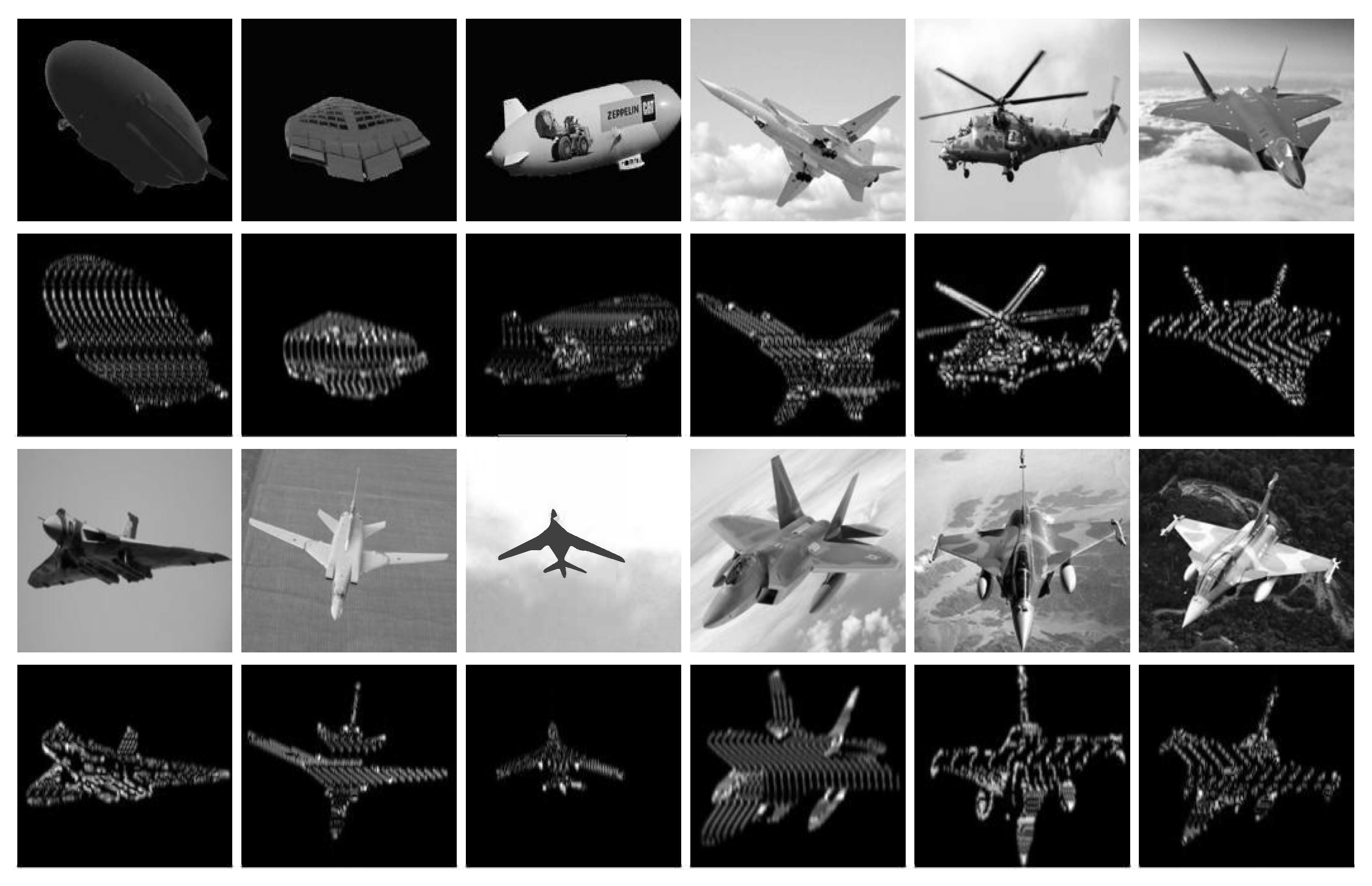
Image fusion has been successfully applied in various fields [7]. However, the fusion sources have mostly been static images such as infrared and visible images, which do not provide dynamic information about the scene. This limitation can be overcome by fusing inverse synthetic aperture radar (ISAR) images with visible images. The fusion of ISAR and visible images yields informative images with detailed and dynamic information from the visible and ISAR images, respectively. The advantages of the fusion of the ISAR and visible images facilitate its application in security surveillance, air traffic control, wildlife conservation, and intelligent assistance [8,9,10,11].

In recent decades, numerous image fusion methods have emerged. The conventional image fusion methods can generally be grouped into three categories [12], namely, spatial domain methods [13,14,15], transform domain methods [16,17,18] and deep-learning-based methods [19]. The spatial domain methods directly operate on the pixel values of the input images and process the image on a pixel-by-pixel basis [20]. These methods have a simple processing flow and strong interpretability, and are widely used in pixel-level image fusion [21]. For example, Wan et al. [22] merged the images using the most significant features of a sparse matrix, which were obtained through the robust principal component analysis. Mitianoudis et al. [14] transformed the images using independent component analysis (ICA) and topographic independent component analysis. Fusion results were obtained in the transform domain using novel pixel-based or region-based rules. Yin et al. [23] proposed a dual-kernel side window box filter decomposition method and a saliency-based fusion rule for image fusion. Smadi et al. [24] adopted side window filtering employed on several filters to decompose and fuse the images. Yan et al. [25] decomposed the images using an edge-preserving filter and refined the final fused image with a guided filter. Zou [26] designed a multiscale decomposition method based on a guided filter and a side window box filter. The spatial-domain methods usually use a symmetric structure to design fusion strategies. However, in cases where there is a large difference in information intensity between the input images, weak signals are often overwhelmed by strong signals, resulting in the loss of some critical details.

The transform domain methods transform the images into another subspace where the features are classified and considered globally [27]. These methods are usually established on some dictionaries or models and can retain more meaningful information [17]. For instance, Liu et al. [27] represented the different components in the original images using sparse coefficients. Zhang et al. [28] represented the images through a multi-task robust sparse representation (MRSR) model, and were able to process the unregistered images. Liu et al. [29] decomposed the images using nonsubsampled shearlet transform (NSST) for pre-fusion. Qu et al. [30] represented the images in a nonsubsampled contour-let transform domain. Furthermore, a dual-pulse coupled neural network (PCNN) model was adopted to fuse the images. Panigrahy et al. [31] transformed images into the NSST domain and fused the images with adaptive dual channel PCNN. Indhumathi et al. [32] transformed the images with empirical mode decomposition (EMD) and then fused them with PCNN. Similarly to spatial-domain methods, transform-domain methods often use the same dictionary or model to extract feature information from images. These transformations use non-local or global information. However, this will lead to the loss of some important but globally less significant information, such as dim targets in infrared images.

Deep-learning-based methods have recently been introduced into the field of image fusion. These methods employ deep features to guide the fusion of two images [7,33]. Most of the deep-learning-based fusion strategies and generation methods report strong scene adaptability [34,35,36]. However, due to down-sampling in the network, the fusion results of deep-learning-based methods are usually blurred.

Although most of the conventional approaches have achieved satisfactory results, these methods fuse the two different source images in the same way. In the ISAR and visible image fusion, objects in the captured scene are mostly stationary or move slowly relative to the radar. As a result, ISAR images have large black backgrounds and many weak signals, while visible images are information-rich. This significant information difference makes conventional symmetric approaches inadequate for processing these images. These approaches will result in the mismatching of feature layers and affect the final fusion performance. For example, in [5], the same decomposition method is applied to both source images. Hence, significant information from these images may be lost during the fusion process. Similarly, in the sparse representation methods [17,27], the same over-complete dictionary is applied to different images, resulting in some features being ignored.

Hence, most conventional approaches cannot deal suitably with the fusion of different images containing quite different information content. Further research is needed on how to balance the differences in information between different source images to preserve as many details as possible. To the best of our knowledge, there are few studies considering the inequality information between two input images. This study aims to balance the information difference between different source images and preserve image details as much as possible in the fusion results. To achieve this objective, we analyzed heterogeneous image data, including ISAR, visible, and infrared data. We found that although the data acquisition methods are different, they describe different information about the same scene. There are some underlying connections between these pieces of information. Therefore, we hypothesized that these pieces of information can be guided and obtained through other source images. Under this assumption and motivated by the work of [5,25], we innovatively designed an asymmetric decomposition method, aiming to use strong signals to guide weak signals. Through the operation, we can obtain potential components from weak signals and enhance them, ensuring that weak signals can be fully preserved in the fusion result.

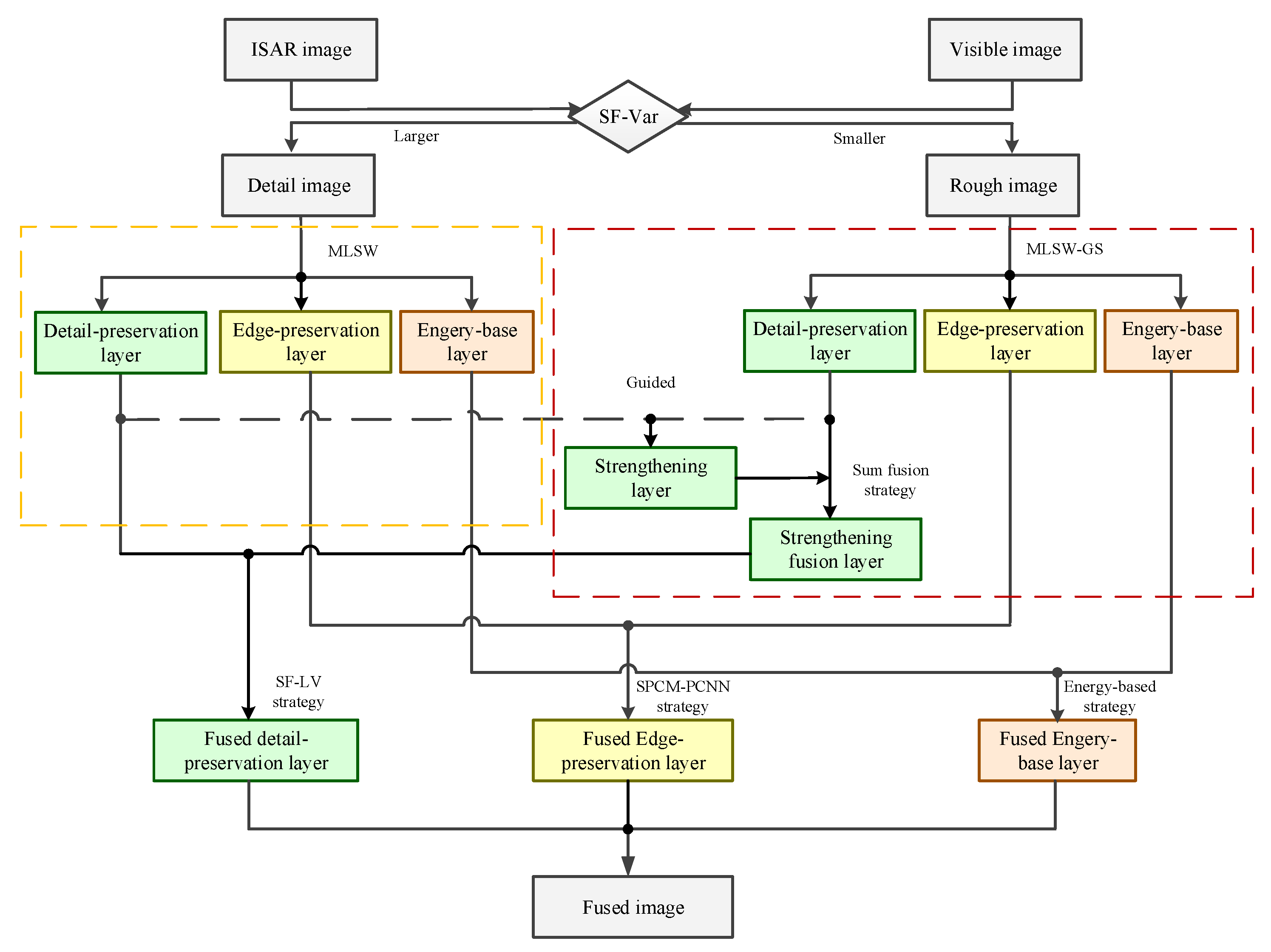
Based on the idea above, under the assumption that the images have been registered at the pixel level, the current research proposes a novel fusion method named the adaptive guided multi-layer side window box filter decomposition (AMLSW-GS) method. Firstly, an information abundance discrimination method is proposed to categorize the input images as detailed and coarse images. Secondly, a novel asymmetric decomposition framework is proposed to decompose the detailed and coarse images, respectively. The detailed image is decomposed into three layers constituting small details, long edges, and base energy. Similarly, the coarse image is used to yield an additional layer containing the strengthening information. Thirdly, a pre-fusion step is adopted to fuse the layers containing strengthening information and the layers containing the small details from the coarse image. Furthermore, three different fusion strategies are adopted to fuse the different layers, and the sub-fusion results are obtained. Finally, the fusion result is obtained as a summation of different sub-fusion results.

The main contributions of the current work are as follows:

(1)

We innovatively propose an asymmetric decomposition method to avoid losing vital information and balance the features of input images.

(2)

We design an information abundance measurement method to justify the amount of information in input images. This measurement estimates the information variance and edge details in the input images.

(3)

We propose three different fusion strategies to use different feature information for different layers. These strategies are designed according to the characteristics of different layers.

(4)

We publicize a pixel-to-pixel co-registered dataset containing visible and ISAR images. To the best of our knowledge, this is the first dataset related to the fusion of visible and ISAR images.

In summary, to address the problem of weak signal loss due to uneven fusion information intensity, under the assumption that the images are already registered at the pixel level and information can be guided, this study proposes an asymmetric decomposition method to enhance the weak signal and ensure the completeness of information in the fusion result. This article is organized as follows. In Section 2, the proposed method is presented in detail. In Section 3, the dataset is introduced and the experimental results on ISAR and VIS images are presented. In Section 4, some characteristics of the proposed method are discussed. In Section 5, we conclude this paper.

2. Proposed Method

In this paper, an ISAR and VIS fusion method based on AMLSW-GS decomposition is proposed. As shown in Figure 1, the ISAR and VIS images are decomposed using the AMLSW-GS method into layers at different scales. For the multi-scale layers, different fusion strategies are adopted to obtain the fusion results at different scales. Finally, the fusion results at different scales are summed together to yield the final fusion result.

2.1. Information Abundance Discrimination

To estimate the information complexity of different input images, a method based on spatial frequency and variance (SF-Var) is proposed. The SF-Var is a global evaluation parameter, which is computed as the weighted average of spatial frequency (SF) and global variance. $SF$ is used to describe the total amount of edges in the images and is computed as

$$RF=\sqrt{\frac{1}{M\times N}\sum _{x=1}^M\sum _{y=2}^N{\left(I\left(x,y\right)-I\left(x,y-1\right)\right)}^2}$$

(1)

$$CF=\sqrt{\frac{1}{M\times N}\sum _{x=1}^M\sum _{y=2}^N{\left(I\left(x,y\right)-I\left(x-1,y\right)\right)}^2}$$

(2)

$$SF=\sqrt{C{F}^2+R{F}^2}$$

(3)

where M and N denote the dimensions of image I, and $RF$ and $SF$ are the row and column frequencies, respectively.

The variance (Var) is a statistical indicator to evaluate the strength of the edges of an image and is computed as

$$Mean=\frac{1}{M\times N}\sum _{x=1}^M\sum _{y=1}^{N}I\left(x,y\right)$$

(4)

$$Var=\frac{1}{M\times N}\sum _{x=1}^M\sum _{y=1}^N{\left(I\left(x,y\right)-Mean\right)}^2$$

(5)

The complexity of the image content is judged based on two types of edge information: edge quantity information derived from SF, and edge intensity information derived from variance. The complexity is then calculated using the weighted average method as

$$SV=\frac{SF\times Var}{SF+Var}$$

(6)

where $SV$ represents the evaluation index of the SF-Var method. The larger the $SV$, the richer the information.

2.2. Decomposition Method

In the conventional decomposition methods, the images are often decomposed in the same manner irrespective of their differences. As the information content of different images is quite different, the conventional methods may lose the image information. In this section, the AMLSW-GS decomposition method will be introduced. Images with different levels of content complexity are decomposed into layers of different scales to avoid information loss. The ISAR and VIS images are decomposed into multi-scale layers using the AMLSW-GS approach. The AMLSW-GS decomposition method comprises two steps, namely, multi-layer Gaussian side window filtering (MLSW) and multi-layer Gaussian side window filtering with guided strengthening (MLSW-GS).

2.2.1. Multi-Layer Gaussian Side Window Filtering

After the image information redundancy is judged, we can distinguish the complexity of the two input images. For the high-complexity image, we employ the multi-layer Gaussian side window filtering (MLSW) decomposition approach, as detailed in Figure 2.

It may be noted that there are two information extraction streams in the MLSW, a Gaussian high-frequency feature extraction stream and a side window high-frequency feature extraction stream. Both of these streams differ in their ability to extract detailed features.

The extraction process of the Gaussian high-frequency features is summarized as

$$I_{gi}=GF\left(I_{g(i-1)}\right)$$

(7)

where $I_{gi}$ is the i-th low frequency information of the Gaussian filter, i = 1, 2, …, n, $I_{g0}=I$. n is the number of decomposition layers. GF() represents the Gaussian filter. In the experiments adopted in this study, the size of the filter window and the standard deviation are set to 3.

The process of side window high-frequency feature extraction is based on the side window filter [37]. The side window filter is an edge-preserving filter, which assumes the edge pixels to have a stronger correlation with the side pixels than the entire neighborhood. Hence, the reconstructed edges will not be too blurred as compared to the other traditional filters. In addition, the side window structure can also be applied to the other traditional filters such as the mean filter, median filter, Gaussian filter, etc. In this research, we adopted the box side window filter as the side window structure.

The process of side window high-frequency feature extraction, using the box side window filter, can be described as

$$I_{di}=SWF(I_{d(i-1)},r,iter)$$

(8)

where $I_{di}$ is the i-th low-frequency information of the side window filter, i = 1, 2, …, n. $I_{d0}$ = I. n is the number of decomposition layers, $SWF\left(\right)$ represents the side window filter [37], r represents the radius of the filter window, and $iter$ represents the number of iterations. In our experiments, we adopted the recommended values given in [37]: $r=1$ and $iter=7$.

Two of the above feature extraction streams yield two different background information images, namely, $I_{gi}$ and $I_{di}$. Both of these contain decreasing detail. The detail preservation layers $D{P}_i$ and the edge preservation layers $E{P}_i$ are then estimated as

$$D{P}_i=I_{g(i-1)}-I_{di},i=1,2,...,n$$

(9)

$$E{P}_i=I_{di}-I_{gi},i=1,2,...,n$$

(10)

The base layer in this framework is the final layer of the Gaussian feature extraction stream $I_{gn}$. It may be noted that in this study, n = 3.

Just as in the work in [5,25], edge-preserving filters are often used for image feature decomposition. They take advantage of the blurring characteristics of edge-preserving filters to remove some of the detailed information from the original image. Detailed information can be obtained by difference operation. The decomposition framework in this section is also based on such filter characteristics. However, two filters with different blur capabilities are used in this section to extract details, so that more detailed information can be extracted from images with different levels of blurring. However, as we know, when the same filter is applied to data with different intensities, the absolute strength of the difference values can also vary, which can cause some weak signals to be overwhelmed by strong signals. This is why we designed another enhanced decomposition framework.

2.2.2. Multi-Layer Gaussian Side Window Filter with Guided Strengthening

To make full use of the two images containing different information, and enhance the characterization of weak signals, we design a decomposition framework called the multi-layer Gaussian side window filter with guided strengthening (MLSW-GS). We apply the MLSW-GS to the low-complexity image which needs to be enhanced. The steps involved in MLSW-GS are summarized in Figure 3.

Based on the MLSW framework, we introduce a guided stream where an image with high-complexity information is used to guide the decomposition of an image with low-complexity information. The guiding process can be described as

$$S_i=Guid(DP{h}_i,DP{l}_i)$$

(11)

where $S_i$ represents the i-th strengthening layer. $DP{h}_i$ represents the i-th detailed layer of MLSW, $DP{l}_{di}$ represents the i-th detailed layer of the MLSW-GS, and i = 1, 2, 3, …. $Guid\left(\right)$ represents the guided filter [38]. $DP{h}_i$ contains complex information, and $DP{l}_{di}$ contains little information. Through this guidance operation, we can relatively enhance the weak details in the low-complexity image layers.

The MLSW-GS yields a new layer called the strengthening layer, in addition to the three type layers obtained using MLSW.

2.3. Fusion Strategies

The AMLSW-GS framework yields different detailed layers for different images. For the image with high-complexity information, the MLSW decomposition method results in detailed preservation layers (DP), edge preservation layers (EP), and a base energy layer (B). For the image with low-complexity information, the MLSW-GS decomposition method yields four layers, namely, the strengthening layers (S), DP layers, EP layers, and base layer.

2.3.1. Fusion Strategy for Strengthening Layers

As the number of layers of the two images is different, pre-fusion processing of the strengthening layers is necessary. The strengthening layers have some enhanced information and the main image structure is similar to that of DP layers. Hence, we carry out a pre-fusion for these two layers; the fusion strategy can be described as

$$SF{L}_i=DP{l}_i+S_i$$

(12)

where $SF{L}_i$ represents the i-th strengthening fusion layer, $DP{l}_i$ represents the i-th detail preservation layer of low complexity, and $S_i$ represents the i-th strengthening layer.

2.3.2. Fusion Strategy for Detail Preservation Layers

Based on Equation (12), the strengthening fusion layers (SFL) were obtained. In detailed preservation layers, small structures and edges are mainly preserved. Therefore, the more small structures that are preserved, the better the fusion result. Based on this principle, the spatial frequency and local variance (SF-LV) fusion strategy is adopted to fuse the SFL layers and the DP layers of the highly complex source. The fusion strategy can be described as

$$FD{P}_i=\left\{\begin{array}{cc}DP{h}_i,& ifSF\left(SF{L}_i\right)<SF\left(DP{h}_i\right)andLV\left(SF{L}_i\right)<LV\left(DP{h}_i\right)\\ SF{L}_i& otherwise\end{array}\right.$$

(13)

where $DP{h}_i$ represents the i-th detail preservation layer of a high-complexity source, $SF{L}_i$ represents the i-th strengthening fusion layer, and $SF(·)$ represents the local spatial frequency, which can be calculated using Equation (1) to Equation (3). The M and N in Equations (1) and (2) represent the size of the local area in the image. $LV(·)$ represents local variance and is calculated as

$$LV(x,y)=\sum _{r=-\frac{P}{2}}^{\frac{P}{2}}\sum _{s=-\frac{Q}{2}}^{\frac{Q}{2}}\frac{{I(x+r,y+s)-\mu }^2}{P\times Q}$$

(14)

where I represents the image, x and y represent the center position of the local image patch, r and s represent the pixel index in the image patch, P and Q represent the size of the image patch, and $\mu$ represents the mean of the pixels in the image patch.

The SF can describe the number of edges in the local area, while the LV can describe the distribution of pixels in the local area. This fusion strategy can describe the local attributes, which is important for locating small structures.

2.3.3. Fusion Strategy for Edge Preservation Layers

In edge preservation layers, long edges with strong intensity are mainly preserved. Therefore, the more accurate the edge location is, the better the fusion result. Based on this principle, a fusion method, named the morphological symmetric phase consistency motivated pulse coupled neural network (SPhCM-PCNN), is proposed to fuse the preservation layers.

Symmetric Phase Consistency

Classic phase consistency (PhC) [39] is an effective method for feature extraction, focused on edge features. Compared with other edge extraction methods, PhC methods have advantages in terms of edge localization and weak edge extraction. However, the approach is not effective when the frequency component of the signal is not rich. In addition, for some sharp edges, such as step edges, the aftershock phenomenon [40] will occur in the boundaries.

Therefore, to avoid the limitations of the PhC method, symmetry phase consistency (SPhC) is adopted. Based on the work of [41,42], symmetrical phase consistency makes use of the symmetry of the signal. Symmetry features can describe the signal features where all of the frequency components are aligned in symmetry and in phase. In the image, the position near the edge often shows strong symmetry or anti-symmetry. By filtering the symmetrical phase in the image, the edge position of the image can be located more quickly and accurately. As only the symmetrical phase is considered, the SPhC method can suppress the aftershock effect to a certain extent.

Classic phase consistency [40] is described by the Fourier series expansion and is calculated as

$$\left\{\begin{array}{c}I\left(x\right)=\sum _n{A}_{n}cos\left({\varphi }_n\left(x\right)\right)\\ PhC\left(x\right)=\underset{\overline{\varphi }\left(x\right)\in [0,2\pi ]}{max}\frac{{\sum }_n{A}_{n}cos({\varphi }_n\left(x\right)-\overline{\varphi }\left(x\right))}{{\sum }_n{A}_n}\end{array}\right.$$

(15)

where the $I\left(x\right)$ is the image signal, and $A_n$ and ${\varphi }_n\left(x\right)$ represent the coefficients and local phase of the n-th Fourier component at location x, respectively. $\overline{\varphi }$(x) is the weighted mean local phase of all the Fourier components at point x.

Equation (15) is hard to calculate. To compute the PhC features, local energy is considered to simplify the process. The local energy is defined as

$$E\left(x\right)=\sqrt{I{\left(x\right)}^2+H{\left(x\right)}^2}$$

(16)

where $H\left(x\right)$ is the Hilbert transform of the I(x). H(x) can generate the 90-degree phase shift of the I(x).

For the one-dimension signal $f\left(x\right)$, supposing that $M_n^e$ and $N_n^o$ are even symmetric filters and odd symmetric filters in the scale n, the odd symmetric filters are 90-degree phase shift filters of the even symmetric filters. We can calculate the strength coefficients of the odd and even filters at position x as

$$[e_n\left(x\right),o_n\left(x\right)]=[f\left(x\right)*M_n^e,f\left(x\right)*N_n^o]$$

(17)

where $e_n\left(x\right)$ and $o_n\left(x\right)$ represent the strength coefficients of the even components and odd components, respectively. * is a convolution operation.

Furthermore, we compute the local amplitude $A_n\left(x\right)$ at the scale n as

$$A_n\left(x\right)=\sqrt{e_n{\left(x\right)}^2+o_n{\left(x\right)}^2}$$

(18)

The local energy $E\left(x\right)$ at position x is calculated as

$$E\left(x\right)=\sqrt{\sum {e_n\left(x\right)}^2+\sum {o_n\left(x\right)}^2}$$

(19)

The phase consistency of the signal $f\left(x\right)$ is computed as

$$PhC\left(x\right)=\frac{E\left(x\right)}{{\sum }_n{A}_n\left(x\right)+ϵ}$$

(20)

where $ϵ$ is a small positive constant to avoid a zero denominator.

For the two-dimensional images, the PhC value is calculated in different directions, and results in all directions being summarized to obtain the PhC value. The phase consistency of the image can be described as

$$Ph{C}_{2D}\left(x\right)=\frac{{\sum }_j{E}_{{\theta }_j}\left(x\right)}{{\sum }_n{\sum }_j{A}_{n{\theta }_j}\left(x\right)+ϵ}$$

(21)

where ${\theta }_j$ is the j-th direction, and ${\theta }_j=j\pi /m,j=0,1,2...,m-1$; here, m = 6.

The phase consistency can locate the edges accurately, but an aftershock phenomenon exists in the phase consistency result [43]. In order to solve this problem, the symmetry of the phase is researched.

Symmetry is a basic element of image features. The edges are often at the most symmetric or asymmetric points in all the frequencies. Hence, we can use these special phases to obtain the image features. In the symmetry phase consistency, we only consider four special phases, $-\pi /2$, 0, $\pi /2$, and $\pi$. These four phases are symmetric and asymmetric at all scales. The $-\pi /2$ and $\pi /2$ are the symmetric phase and the 0 and $\pi$ are the asymmetric phase. Hence, the symmetric phase consistency can be described as

$$\left\{\begin{array}{c}SPhC\left(x\right)=\frac{SumE\left(x\right)}{SumA\left(x\right)+ϵ}=\frac{\sqrt{{\displaystyle \sum _{k,q}}{e}_{n\left(k\right),\theta \left(q\right)}{\left(x\right)}^2+{\displaystyle \sum _{k,q}}{o}_{n\left(k\right),\theta \left(q\right)}{\left(x\right)}^2}}{{\displaystyle \sum _{k,q}}\sqrt{e_{n\left(k\right),\theta \left(q\right)}{\left(x\right)}^2+o_{n\left(k\right),\theta \left(q\right)}{\left(x\right)}^2}+ϵ}\\ {\varphi }_{n\left(k\right),\theta \left(q\right)}\in \left\{-\pi /2,0,\pi /2,\pi \right\}\end{array}\right.$$

(22)

where SPhC(x) represents the symmetric phase consistency at point x. $SumE\left(x\right)$ and $SumA\left(x\right)$ represent the sum of local energy and the sum of local amplitude in ${\varphi }_{n\left(k\right),\theta \left(q\right)}$. ${\varphi }_{n\left(k\right),\theta \left(q\right)}$ is the symmetric phase, $n\left(k\right))$ and $\theta \left(q\right)$ are the scale and the orientation, and $k,q=0,1,2...$. $e_{n\left(k\right),\theta \left(q\right)}\left(x\right)$ and $o_{n\left(k\right),\theta \left(q\right)}\left(x\right)$ represent the strength coefficients of the even components and odd components at scale $n\left(k\right)$ and orientation $\theta \left(q\right)$, respectively.

There are some noises that may affect the estimation of the fusion weights. Therefore, we add a morphological operation before the symmetric phase consistency. Furthermore, we obtain the morphological symmetric phase consistency result as

$$SPhCM\left(x\right)=\sum _{t=1}^N{\omega }_t·(SPhC\left(x\right)\oplus S{E}_t-SPhC\left(x\right)\ominus S{E}_t)$$

(23)

where $S{E}_t$ donates a basic structure element at t scale, t = 1, 2, 3, …, N. Here, N = 3. ⊕ and ⊖ represent the morphological dilation and erosion operations. ${\omega }_t$ represents the t-scale weight. It can be calculated by

$${\omega }_t=\frac{1}{2t+1}$$

(24)

Morphological Symmetric Phase Consistency Motivated Pulse Coupled Neural Network

In order to locate the edge accurately, the SPhCM-PCNN transforms the classical PCNN [44] model to the phase consistency domain. The SPhCM-PCNN framework is summarized in Figure 4

The main fusion framework of SPhCM-PCNN is a two-channel PCNN model. It can be calculated as

$$F_{ij}^1\left(k\right)=S_{ij}^1\left(k\right)$$

(25)

$$F_{ij}^2\left(k\right)=S_{ij}^2\left(k\right)$$

(26)

$$L_{ij}\left(k\right)=\left\{\begin{array}{cc}1,& if{\displaystyle \sum _{r,t\in S}}{Y}_{rt}(k-1)>0\\ 0,& otherwise\end{array}\right.$$

(27)

$$U_{ij}\left(k\right)=max\left\{F_{i,j}^1\left(k\right)\left(1+{\beta }_{i,j}^1{L}_{ij}\left(k\right)\right),F_{ij}^2\left(k\right)\left(1+{\beta }_{ij}^2{L}_{ij}\left(k\right)\right)\right\}$$

(28)

$$Y_{ij}\left(k\right)=\left\{\begin{array}{cc}1,& if{U}_{ij}\left(k\right)>={\theta }_{ij}(k-1)\\ 0,& otherwise\end{array}\right.$$

(29)

$${\theta }_{ij}\left(k\right)={\theta }_{ij}(k-1)-\mathrm{\Delta }+V_{\theta }{Y}_{ij}\left(k\right)$$

(30)

$$T_{ij}\left(k\right)=\left\{\begin{array}{cc}k,& if{U}_{ij}\left(k\right)>={\theta }_{ij}(k-1)\\ T_{ij}(k-1),& otherwise\end{array}\right.$$

(31)

where $S_{ij}^1$ and $S_{ij}^2$ represent the pixels of the two images at point (i, j). The source images are edge preservation layers from the ISAR and visible images. $L_{ij}$ represents the link parameter. ${\beta }_{ij}^1$ and ${\beta }_{ij}^2$ represent the link strength. $F_{ij}^1$ and $F_{ij}^2$ represent the input feedback. $U_{ij}$ is the output of the dual channels. ${\theta }_{ij}$ is the threshold of the step function. $Y_{ij}\left(k\right)$ is the the k-th iteration output of PCNN. $\mathrm{\Delta }$ is the value of the threshold decline, and $V_{\theta }$ represents the learning rate of the threshold. $T_{ij}$ represents the criterion that determines the number of iterations. S represents the neighborhood of the pixel at position (i, j).

Based on the dual-channel PCNN above, we replace the ${\beta }_{ij}^1$ and ${\beta }_{ij}^2$ with the results of SPhCM from the two sources. Furthermore, we obtain the fusion map of the edge preservation layers as

$$FE{P}_i=WEP{h}_i\times EP{h}_i+(1-WEP{h}_i)\times EP{l}_i$$

(32)

where $FE{P}_i$ represents the i-th fusion result of the edge preservation layers. $WEP{h}_i$ is the output weight of the SPhCM-PCNN, which has been normalized. $EP{h}_i$ and $EP{l}_i$ are the edge preservation layers of the high-complexity source and the low-complexity source.

2.3.4. Fusion Strategy for Base Layers

The base layers of both the images contain significant energy but lack high-frequency details. Hence, we adopted energy-based methods to fuse the energy layers.

The energy-based methods are summarized as

$$FB(x,y)=\frac{Bh{(x,y)}^2+Bl{(x,y)}^2}{Bh(x,y)+Bl(x,y)}$$

(33)

where the $FB(x,y)$ represents the fusion result of base layers at point (x,y). $Bh$ and $Bl$ are the base layer of the high and low complexity sources.

Finally, all the sub-fusion results are added to obtain the final fusion result:

$$F=\sum _{i=1}^n(FD{P}_i+FE{P}_i)+FB$$

(34)

where n represents the number of decomposition layers. Here, n = 3.

3. Experimental Results

The details of our dataset are discussed in Section 3.1. The qualitative and quantitative comparisons of the proposed method with the other state-of-the-art methods are presented in Section 3.2. The ISAR and visible dataset used in this study were obtained from different sources. The visible images were collected from the Internet [45]. The ISAR images were generated through simulations from the visible images, the details of which are explained in Section 3.1. All experiments were performed using Matlab 2022b by MathWorks, the United States. The computer used for experiments was equipped with an Intel Core i9-12900H CPU, 16 GB of memory produced by Samsung South Korea, and a 512 GB solid-state drive produced by Toshiba Japan.

3.1. ISAR and Visible Dataset

The dataset that we published as a part of this research constitutes co-registered visible and simulated ISAR images. A few examples of the images from the dataset are shown in Figure 5.

All the visible images in the dataset were collected from the Internet [45]. The ISAR images were simulated based on the visible images. The simulation process for ISAR image generation is summarized below:

1.

The targets in the visible images are labeled pixel by pixel; therefore, we can accurately locate the target area.

2.

We set the background pixel values to 0 and only keep the pixels in the target area.

3.

The 3D models of the targets are established to estimate the distance.

4.

The Range Doppler algorithm [46] is adopted to synthesize the ISAR data. To reduce the amount of computation, we resize the images to $151\times 151$.

For the pixel-to-pixel registration, we aligned the visible images to the center of the simulated ISAR images by resizing them to $151\times 151$.

In our dataset, the scenes of visible images are mainly aerial scenes. The targets are moving in the air and near space, including planes, fighters, bombers, and airships. The dataset contains 100 different registered image pairs and 500 more visible images for future target recognition applications. In addition, all of the images containing targets are labeled in the PASCAL Visual Object Classes (PASCAL VOC) format. This provides the possibility to use the dataset for fusion detection tasks.

3.2. Comparison with State-of-the-Art Methods

To demonstrate the superiority of the proposed method, we compared it with fifteen state-of-the-art methods: adaptive sparse representation fusion (ASR) [17], multi-layer decomposition based on latent low-rank representation (MDLatLRR) [47], anisotropic diffusion, and the Karhunen–Loeve transform fusion (ADF) [48,49]; the fourth order partial differential equation fusion (FPDE) [50]; fast multi-scale structural patch decomposition-based fusion (FMMEF) [51]; night-vision context enhancement fusion (GFCE) [52]; visual saliency map and weighted least square optimization fusion (VSMWLS) [53]; Gradientlet [54]; latent low-rank representation fusion (LatLRR) [16]; pulse-coupled neural networks in non-subsampled shearlet transform domain fusion (NSCT-PAPCNN) [18]; spatial frequency-motivated pulse-coupled neural networks in non-subsampled contourlet transform domain fusion (NSCT-SF-PCNN) [30]; multi-scale transform and sparse representation fusion (MST-SR) [27]; guided-bilateral filter-based fusion in wavelet domain (DWT-BGF) [55]; VGG19-L1-Fusion [19]; and Image Fusion with ResNet and zero-phase component analysis (ResNet50-ZPCA) [56]. Eight metrics have been adopted to evaluate the quality of the fusion results, namely, the Mutual information (MI) [57], Nonlinear Correlation Information Entropy (NCIE) [58], Objective Evaluation of Fusion Performance ($Q_{ab/f}$) [59], Fusion Quality Index ($Q_S$) [60], Disimilarity-based quality metric ($Q_Y$) [61], Average, Structural Similarity (SSIM), and Feature Mutual Information (FMI) [62,63].

For the subjective evaluation, four examples of image pairs with their fusion results, using different methods, are shown in Figure 6, Figure 7, Figure 8 and Figure 9.

As shown in Figure 6, the fusion source images contain planes with clouds in the background. There is some scene information in the visible source and some speed information of the plane in the ISAR source. The fusion result should contain both of these sources of information as much as possible. For the results of the MDLatLRR, FPDE, Gradientlet, LatLRR, DWT-BGF, VGG19-L1-Fusion, and ResNet50-ZPCA methods, the details of the ISAR information are blurred, which is marked by the red box. This means that these methods lose some high-frequency information. This phenomenon occurs because these methods use the same decomposition framework, and decompose the visible image and ISAR image at the same level. However, in this scene, the average brightness of the visible image is significantly higher than that of the ISAR image. This causes the details of the ISAR image to be treated as noise and submerged in the visible information. As a result, the ISAR information is lost. For the methods of the ASR, ADF, FMMEF, GFCE, VLMWLS, and the MST-SR methods, the area marked by the red box shows more ISAR information. However, these approaches ignore the information from the VIS source. This is because the scene brightness of the ISAR is significantly lower than that of the visible image. Therefore, when performing fusion operations, the brightness of the visible image changes significantly due to the influence of the ISAR brightness, causing signal strength loss. Benefiting from the asymmetric decomposition framework, our proposed method can preserve the ISAR details while maintaining visible information. Most of the fusion results suppress the background intensity of the visible scene, which is marked by the green box. Some of the results, such as those for the NSCT-SF-PCNN and MST-SR methods, have uneven background and block effects. Our proposed method and the NSCT-PAPCNN method preserve the visible source information. In summary, the proposed method yields a better performance as compared to the other methods in terms of fusion quality.

In Figure 7, the fusion details of ISAR and visible sources are marked by red boxes. The visible background area is marked by green boxes. The red-marked areas have been up-sampled by a factor of two and placed in the upper right corner of the images to show the fusion details. The green marked areas aim to show the fused scene brightness. Due to the dark background and lower detail of the ISAR image, the brightness of the green areas indicates the amount of energy retained in the visible scene. The clearer the red areas and the brighter the green areas, the better the fusion result. We can see that the red areas are blurry in the results of the ASR, MDLatLRR, ADF, FPDE, Gradientlet, MST-SR, DWT-BGF, VGG19-L1-Fusion, and ResNet50-ZPCA methods. Only the results of the NSCT-PAPCNN and MST-SR methods and the proposed methods have a well-lit scene in the green area. However, there are artifacts around the plane in the results of the NSCT-PAPCNN method, and the background is not uniform in the results of the MST-SR method. Therefore, compared with the other methods, our proposed method obtained satisfactory fusion results.

In Figure 8, the subjective evaluations are the same as those discussed in the previous case. We can find that the fusion details, marked by the red bounding box, are not clear in the results of the ASR, MDLATLRR, ADF, FPDE, Gradientlet, LatLRR, DWT-BGF, VGG19-L1-Fusion, and ResNet50-ZPCA methods. The details in the NSCT-SF-PCNN and MST-SR methods are clear, but the fusion background is not uniform. The fusion scene marked by green is brighter in the results of the FMMEF, GFCE, NSCT-PAPCNN and proposed methods. Hence, the proposed method and FMMEF, GFCE, and NSCT-PAPCNN methods yield good performance for this scene.

In Figure 9, the edges in the red area are not obvious in the ASR, MDLATLRR, ADF, FPDE, FMMEF, Gradientlet, LatLRR, DWT-BGF, VGG19-L1-Fusion, and ResNet50-ZPCA methods. This means that the information on the ISAR is not fully preserved. The background marked by green is not clear in almost all the contrast-based methods, except for the GFCE and MST-SR methods. The results for the GFCE, LATLRR, NSCT-PAPCNN, NSCT-SF-PCNN, and MST-SR methods have relatively more artifacts around the plane due to the low resolution and noise. Compared with other methods, our proposed method has more details and high contrast. It preserves the information of the two sources as much as possible in this scene. As is evident from Figure 6, Figure 7, Figure 8 and Figure 9, our proposed method has a better performance in most of the scenes in comparison with the state-of-the-art methods.

For the objective evaluation, eight metrics of fusion results are shown in

Table 1. Objective values of different fusion methods in scene 1. The best values, the second-best values, and the third-best values are marked in red, blue, and green, respectively.

Metrics	MI	NCIE	${\mathit{Q}}_{\mathbf{ab}/\mathit{f}}$	${\mathit{Q}}_{\mathit{S}}$	${\mathit{Q}}_{\mathit{Y}}$	Average	SSIM	FMI
ASR	0.5578	0.8084	0.5769	0.6464	0.6187	104.2598	0.8041	0.4333
MDLatLRR	0.5854	0.8093	0.5353	0.6504	0.6027	104.8293	0.8297	0.4230
ADF	0.5917	0.8086	0.3560	0.6050	0.3951	104.2560	0.7582	0.4062
FPDE	0.5904	0.8088	0.3475	0.6168	0.4046	104.6114	0.7809	0.4011
FMMEF	0.3883	0.8057	0.3930	0.7411	0.4927	151.5003	0.9098	0.2929
GFCE	0.3945	0.8055	0.4446	0.6881	0.5477	127.9703	0.8381	0.3334
VSMWLS	0.5542	0.8086	0.5202	0.6559	0.5670	106.5852	0.8169	0.4269
Gradientlet	0.6013	0.8113	0.6105	0.6392	0.6227	106.7499	0.8115	0.4492
LatLRR	0.4850	0.8070	0.5188	0.6727	0.5955	117.1027	0.8406	0.3852
NSCT-PAPCNN	0.5639	0.8094	0.5125	0.7160	0.6102	194.6775	0.8617	0.3737
NSCT-SF-PCNN	0.3335	0.8049	0.2128	0.3642	0.2935	58.5017	0.5315	0.2337
MST-SR	0.3718	0.8061	0.3425	0.6630	0.4895	149.4948	0.8128	0.2777
DWT-BGF	0.5917	0.8094	0.3395	0.5966	0.4214	104.2574	0.7516	0.3527
VGG19-L1-Fusion	0.6139	0.8099	0.3937	0.6219	0.4810	104.3685	0.7949	0.3896
ResNet50-ZPCA	0.6144	0.8099	0.4529	0.6359	0.5367	104.5281	0.8159	0.3980
Proposed	0.8958	0.8238	0.7312	0.7687	0.8584	194.9641	0.9583	0.4929

,

Table 2. Objective values of different fusion methods in scene 2. The best values, the second-best values, and the third-best values are marked in red, blue, and green, respectively.

Metrics	MI	NCIE	${\mathit{Q}}_{\mathbf{ab}/\mathit{f}}$	${\mathit{Q}}_{\mathit{S}}$	${\mathit{Q}}_{\mathit{Y}}$	Average	SSIM	FMI
ASR	0.6830	0.8082	0.5780	0.5889	0.5707	110.0905	0.7903	0.5250
MDLatLRR	0.6905	0.8080	0.5859	0.5988	0.5294	110.7254	0.8068	0.5460
ADF	0.6988	0.8077	0.4831	0.5708	0.3093	110.0439	0.7544	0.5403
FPDE	0.6241	0.8073	0.4608	0.5340	0.4894	110.4954	0.7288	0.4680
FMMEF	0.4761	0.8064	0.2817	0.6797	0.3985	151.6105	0.8842	0.2470
GFCE	0.4652	0.8063	0.3166	0.5693	0.3774	111.7259	0.7319	0.2891
VSMWLS	0.6880	0.8082	0.5552	0.5955	0.5136	109.9762	0.7898	0.5218
Gradientlet	0.7462	0.8099	0.6217	0.5890	0.5791	114.3728	0.7979	0.5601
LatLRR	0.5149	0.8061	0.4308	0.6052	0.4206	127.3659	0.7987	0.3742
NSCT-PAPCNN	0.4937	0.8065	0.2790	0.6085	0.3434	199.6688	0.7669	0.2563
NSCT-SF-PAPCNN	0.3281	0.8048	0.1778	0.3351	0.2678	62.2404	0.5088	0.1991
MST-SR	0.4139	0.8060	0.2486	0.5833	0.3345	145.8304	0.7577	0.2367
DWT-BGF	0.6813	0.8078	0.4721	0.5515	0.3389	110.0405	0.7366	0.5045
VGG19-L1-Fusion	0.7195	0.8081	0.5032	0.5778	0.4063	110.2947	0.7777	0.5455
ResNet50-ZPCA	0.7102	0.8081	0.5430	0.5884	0.4677	110.3883	0.7984	0.5468
Proposed	0.9430	0.8153	0.7210	0.7048	0.8719	201.6202	0.9390	0.6030

,

Table 3. Objective values of different fusion methods in scene 3. The best values, the second-best values, and the third-best values are marked in red, blue, and green, respectively.

Metrics	MI	NCIE	${\mathit{Q}}_{\mathbf{ab}/\mathit{f}}$	${\mathit{Q}}_{\mathit{S}}$	${\mathit{Q}}_{\mathit{Y}}$	Average	SSIM	FMI
ASR	0.5199	0.8085	0.6887	0.7018	0.7696	64.4522	0.8593	0.4409
MDLatLRR	0.5593	0.8094	0.5837	0.6968	0.7141	64.7219	0.8640	0.3938
ADF	0.5277	0.8086	0.6331	0.6865	0.7551	64.4705	0.8692	0.4146
FPDE	0.5323	0.8086	0.5904	0.6910	0.7327	64.8131	0.8684	0.4004
FMMEF	0.5109	0.8084	0.7634	0.8206	0.8713	93.7231	0.9696	0.4511
GFCE	0.4016	0.8058	0.6082	0.7767	0.7982	131.0607	0.9113	0.4097
VSMWLS	0.5319	0.8085	0.6305	0.7190	0.7422	72.1218	0.8782	0.4065
Gradientlet	0.5259	0.8082	0.6345	0.7280	0.7850	76.4990	0.9029	0.4077
LatLRR	0.5837	0.8101	0.6253	0.7336	0.7452	78.2487	0.8876	0.3974
NSCT-PAPCNN	0.6073	0.8123	0.6867	0.8146	0.8360	116.8993	0.9553	0.4181
NSCT-SF-PAPCNN	0.3836	0.8052	0.3798	0.4810	0.4773	65.1187	0.7016	0.3191
MST-SR	0.6663	0.8152	0.7300	0.8199	0.8650	112.0820	0.9570	0.4472
DWT-BGF	0.4827	0.8069	0.2474	0.5287	0.4100	64.4823	0.6754	0.1920
VGG19-L1-Fusion	0.5609	0.8090	0.2814	0.5882	0.4822	64.6862	0.7504	0.2689
ResNet50-ZPCA	0.5608	0.8091	0.3675	0.6389	0.5931	64.6397	0.8052	0.3074
Proposed	0.8304	0.8259	0.7911	0.8374	0.9289	115.1581	0.9930	0.4723

and

Table 4. Objective values of different fusion methods in scene 4. The best values, the second-best values, and the third-best values are marked in red, blue, and green, respectively.

Metrics	MI	NCIE	${\mathit{Q}}_{\mathbf{ab}/\mathit{f}}$	${\mathit{Q}}_{\mathit{S}}$	${\mathit{Q}}_{\mathit{Y}}$	Average	SSIM	FMI
ASR	0.4185	0.8073	0.6167	0.7160	0.7764	74.3090	0.9411	0.4506
MDLatLRR	0.4329	0.8078	0.5032	0.6947	0.7093	74.7527	0.9545	0.4069
ADF	0.4248	0.8077	0.4978	0.6491	0.7113	74.3117	0.9516	0.4100
FPDE	0.4200	0.8076	0.4827	0.6587	0.7078	74.7938	0.9520	0.4061
FMMEF	0.4799	0.8094	0.6492	0.7794	0.8293	101.8566	0.9976	0.4448
GFCE	0.4179	0.8075	0.5518	0.7132	0.7505	146.7715	0.9015	0.4188
VSMWLS	0.4820	0.8093	0.5415	0.7366	0.7766	90.6922	0.9657	0.4238
Gradientlet	0.4863	0.8097	0.5452	0.7308	0.7662	93.1908	0.9916	0.4127
LatLRR	0.4524	0.8082	0.5471	0.7228	0.7422	94.6153	0.9577	0.4114
NSCT-PAPCNN	0.5142	0.8107	0.6215	0.7776	0.8176	124.6620	0.9840	0.4386
NSCT-SF-PAPCNN	0.3983	0.8068	0.4955	0.6745	0.7196	99.2678	0.8855	0.3881
MST-SR	0.5721	0.8137	0.6742	0.7938	0.8555	121.4513	0.9970	0.4671
DWT-BGF	0.3835	0.8065	0.2587	0.5273	0.4725	74.3525	0.7672	0.2277
VGG19-L1-Fusion	0.4422	0.8079	0.3182	0.6100	0.5666	74.7953	0.8771	0.3304
ResNet50-ZPCA	0.4407	0.8080	0.3671	0.6436	0.6258	74.4457	0.9147	0.3525
Proposed	0.6552	0.8179	0.6667	0.7959	0.8718	124.4961	1.0209	0.4516

, where the best values, the second-best values, and the third-best values are marked in red, blue, and green, respectively.

As is evident from Table 1, Table 2, Table 3 and Table 4, the proposed method achieves the best values for all the evaluation metrics. In some cases, even if not the best, the proposed approach achieves the second- or third-best position, as summarized in Table 3 and Table 4. Hence, in view of objective metrics, our proposed method achieves the best performance compared to the other state-of-the-art methods.

To demonstrate the adaptability of the proposed method to different scenes, we conducted experiments on the datasets containing dozens of representative scenes and evaluated them with the eight metrics above. The results for the different methods are shown in Figure 10.

In all the evaluation metrics, a higher value indicates better performance. As shown in Figure 10, our proposed method, which is denoted using a red line, consistently achieves a top-ranked performance across most fusion scenes. These results demonstrate that the proposed method has strong adaptability to different scenarios.

4. Discussion

To further analyze the characteristics and applicability of the proposed method, some experiments were carried out in this section.

4.1. Parameter Analysis of the Proposed Method

In this section, we discuss the impact of parameters on the performance of the method. In the proposed method, many parameters need to be set: the number of decompositions s, the size of the guided filter k, the number of iterations in PCNN L, the number of scales in SPhC l, and the number of scales in morphological operation t. After conducting experiments, we found that the parameters that have a significant impact on the performance of the method are the number of decompositions s and the number of scales in morphological operation t. Hence, we mainly discuss the impact of these two parameters on the performance of the method.

In our experiments, we used the method of controlling the variables to explore. Except for the two parameters being explored, the values of the other parameters were set as follows: $k=3$, $L=200$, and $l=4$. For convenience of analysis, we chose MI and $Q_{ab/f}$ as the metrics for evaluating the performance.

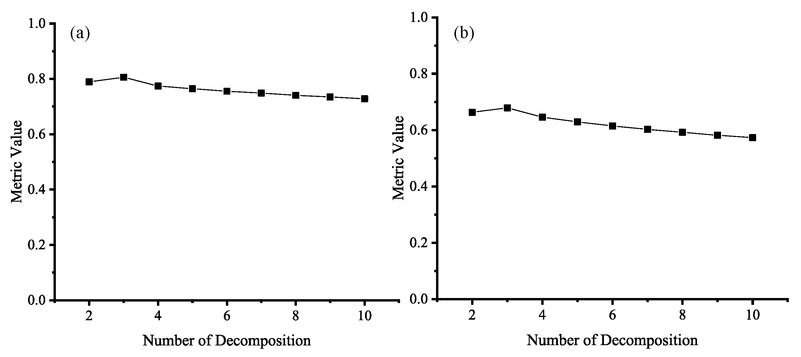
As shown in Figure 11, as the number of decompositions increases, both MI and $Q_{ab/f}$ show an increase followed by a decrease. The best number of decompositions is 3. This is mainly due to the fact that at lower decomposition levels, details can be better distinguished to improve the performance of the fusion result with the increase in the number of decompositions. However, when the number of decompositions is too large, weak details are overly enhanced, resulting in a decrease in the structural similarity of the final fusion result with the input images. The enhancement operations can lead to information imbalance.

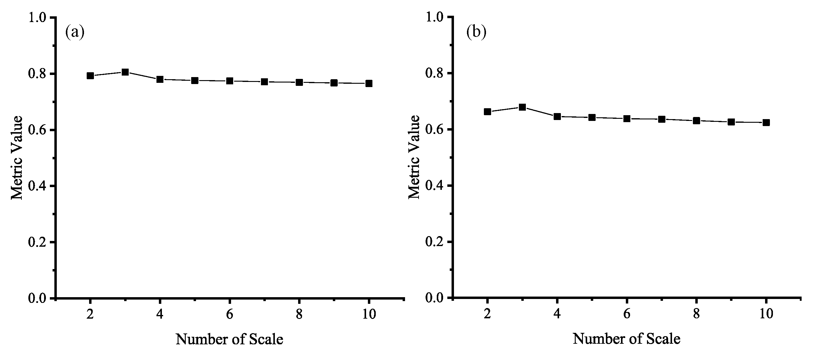
As shown in Figure 12, while the number of scales increases, both MI and $Q_{ab/f}$ also show an increase followed by a decrease. The best number on the scale is 3. This is due to the fact that when the number of scales is small, the multi-scale morphological operation can well locate the position of the object compared to the edge, which improves the final fusion performance. However, when the number of scales is large, due to the characteristics of the morphological operators, there will be more artifacts in the fusion weights, leading to incorrect weight allocation in the areas around the edges, resulting in poorer fusion results.

In summary, the adaptability and the stability of the parameters in the proposed method are weak. Our method performs better with fewer decomposition layers and morphological scales. This is because an increase in the number of layers results in the excessive enhancement of weak signals, and increasing the number of morphological scales results in the inaccurate location of the edges. Both factors will lead to decreased performance. Hence, to further improve the stability of the parameters, we need to further study the internal mechanism of the enhancement, and design a more effective enhancement method to achieve better performance.

As analyzed above, we chose $s=3$ and $t=3$ under consideration of the effectiveness and efficiency of the method.

4.2. Ablation Analysis of the Structure

To verify the effectiveness of the proposed asymmetric method, we conducted some experimental studies in this section.

Based on the analysis of the proposed method, we believe that the factors that mainly affect the fusion performance are concentrated in two aspects: the asymmetric decomposition framework and the selection of fusion strategies. Hence, we analyzed these aspects in this section. The fusion strategy for the energy layer is a classic weighted fusion, so we do not intend to discuss this fusion strategy in this section.

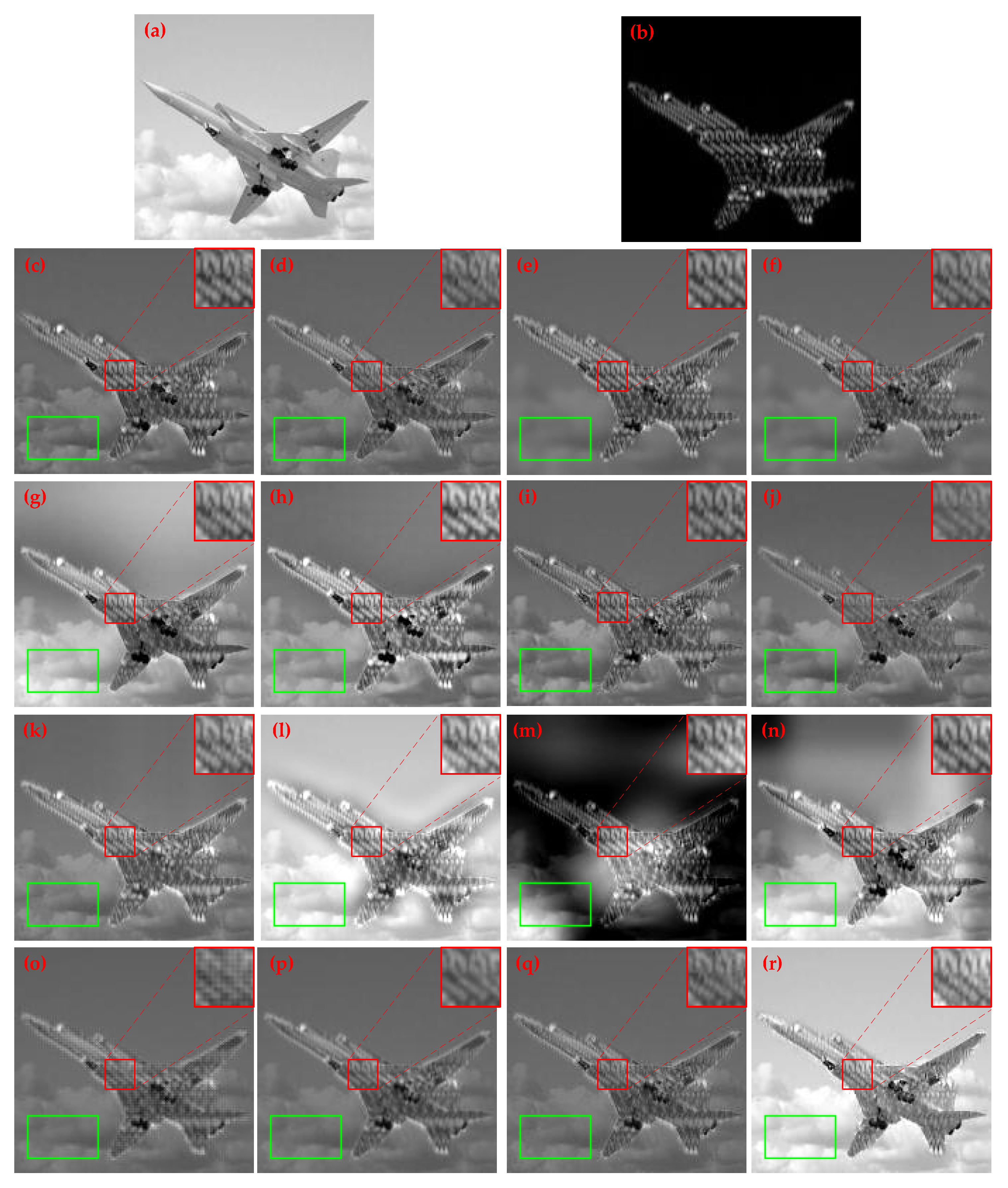
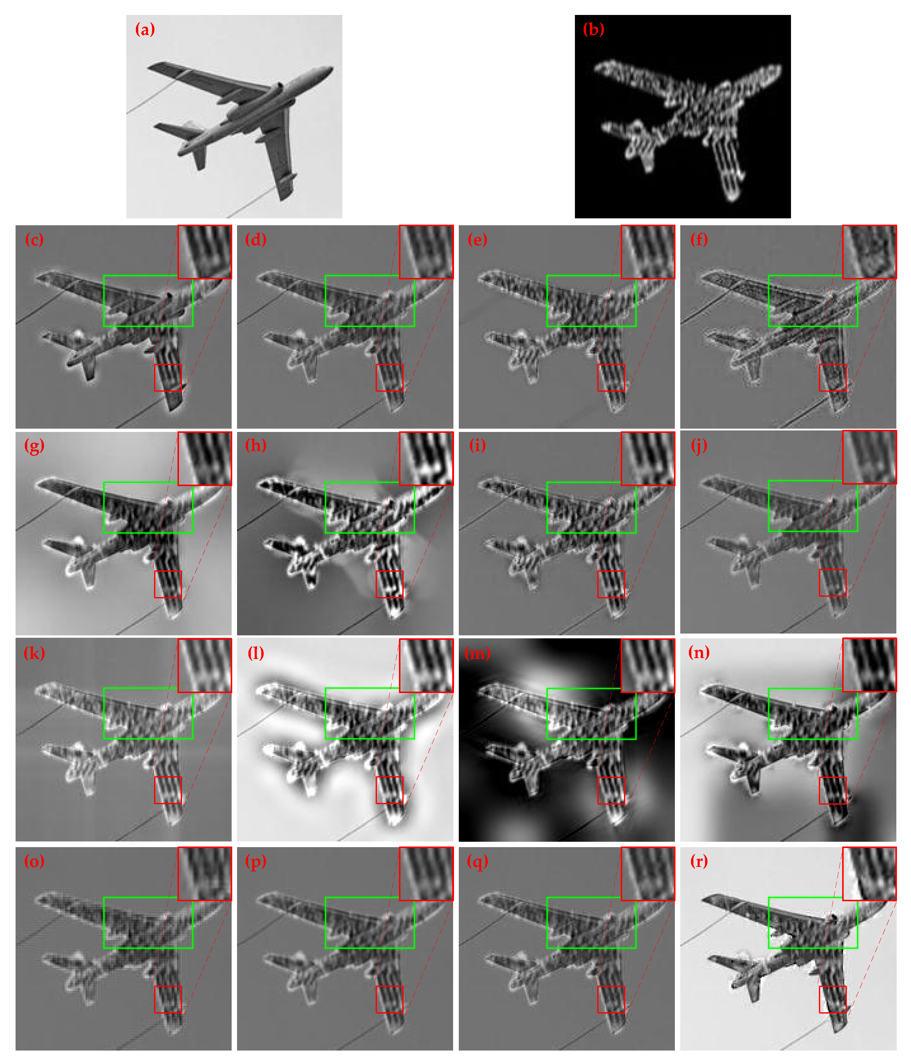
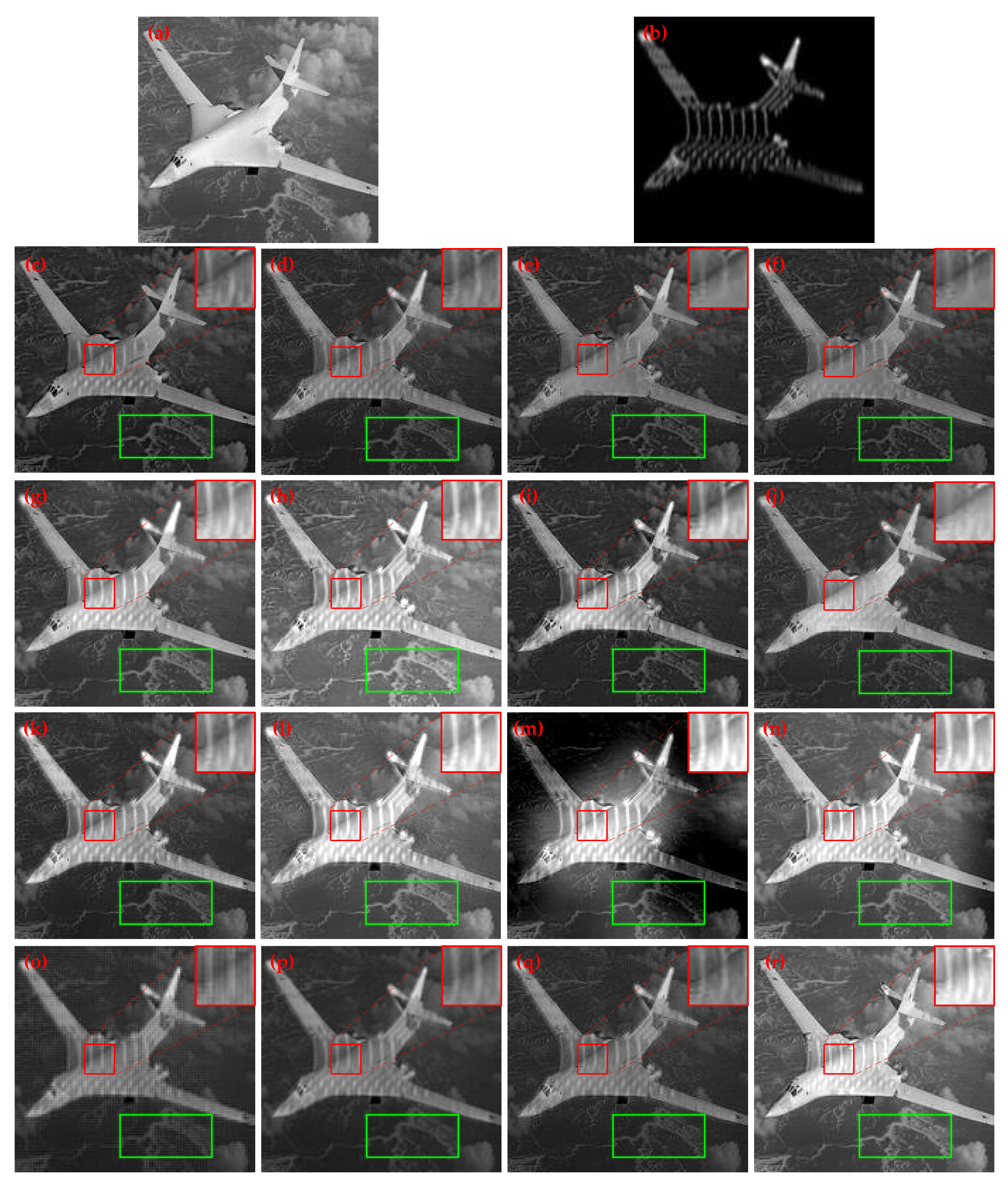
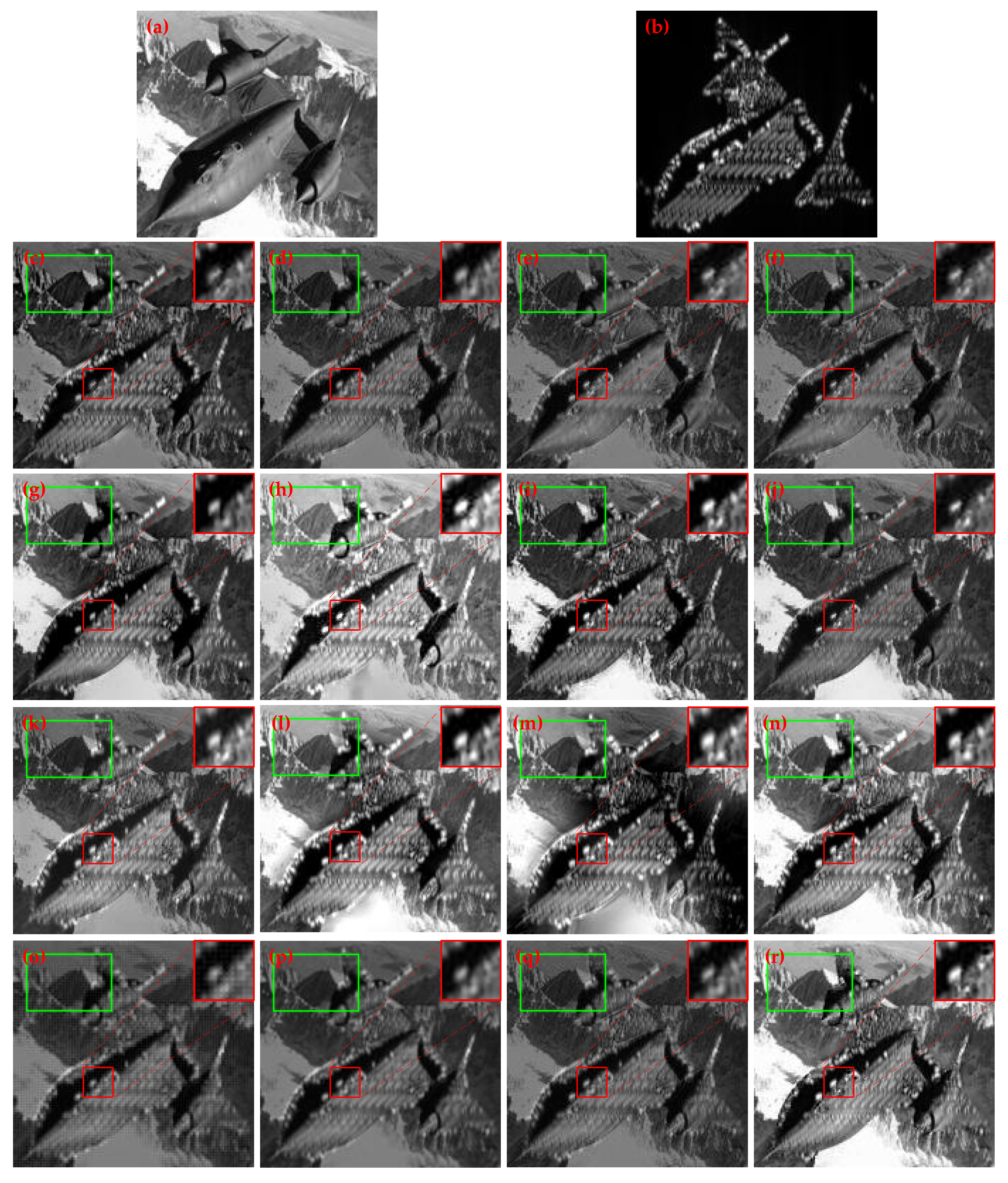
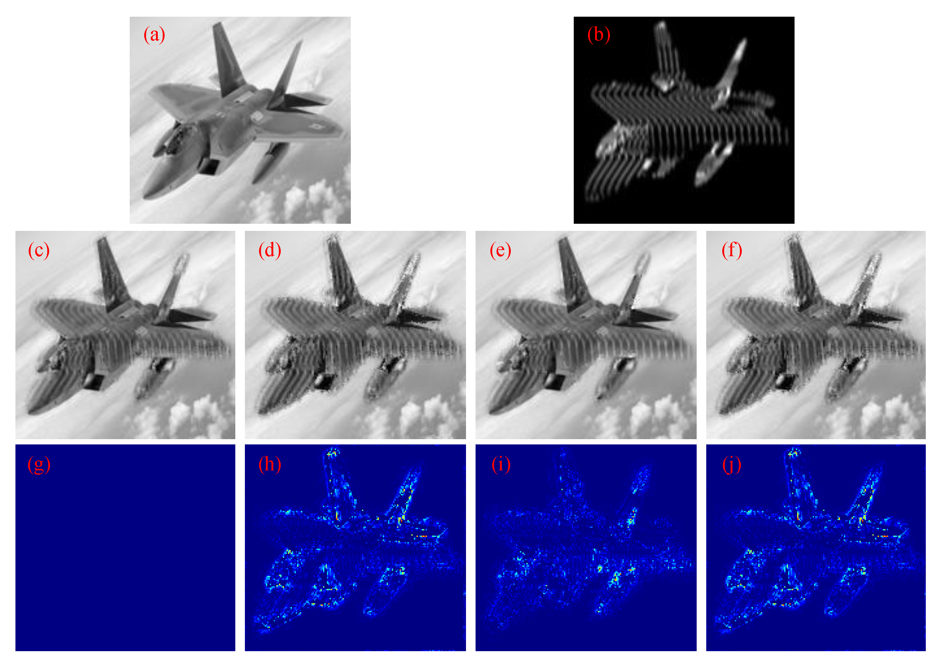
In the experiments, three different structures are discussed and four metrics including MI, NCIE, $Q_{ab/f}$, and SSIM are adopted. The proposed method is denoted as AMLSW + SP + SL, where AMLSW represents the asymmetric decomposition framework we proposed, SP represents the SPhCM-PCNN fusion strategy, and SL represents the SF-LV fusion strategy. Meanwhile, we use MLSW to represent the symmetric decomposition strategy, which replaces MLSW-GS in AMLSW with MLSW. AMLSW + SP represents the decomposition method being AMLSW, and the fusion strategies for detail preservation layers and edge preservation layers are SPhCM-PCNN. AMLSW + SL represents the decomposition method being AMLSW, and the fusion strategies for detail preservation layers and edge preservation layers are SF-LV. The experimental results are shown in Figure 13.

Through Figure 13, we can find that by replacing the decomposition method with a symmetric one, which is shown in Figure 13d,h, some potential information about detail is lost, causing signal distortion in certain areas. This indicates that our asymmetric decomposition structure has the ability to preserve weak signals compared to the symmetric structure. By replacing the detail preservation fusion strategy with SPhCM-PCNN, which is shown in Figure 13e,i, we can find that some small structures and details are lost. This indicates that SF-LV has a better fusion performance on small structures and details, and can better preserve the details of small structures compared to SPhCM-PCNN. By replacing the edge preservation fusion strategy with SF-LV, which is shown in Figure 13f,j, we can find that some long edges are blurred. This indicates that SPhCM-PCNN has a better fusion performance for long edge preservation due to its high precision in edge localization, and that SPhCM-PCNN can better preserve the details of long edges compared to SF-LV.

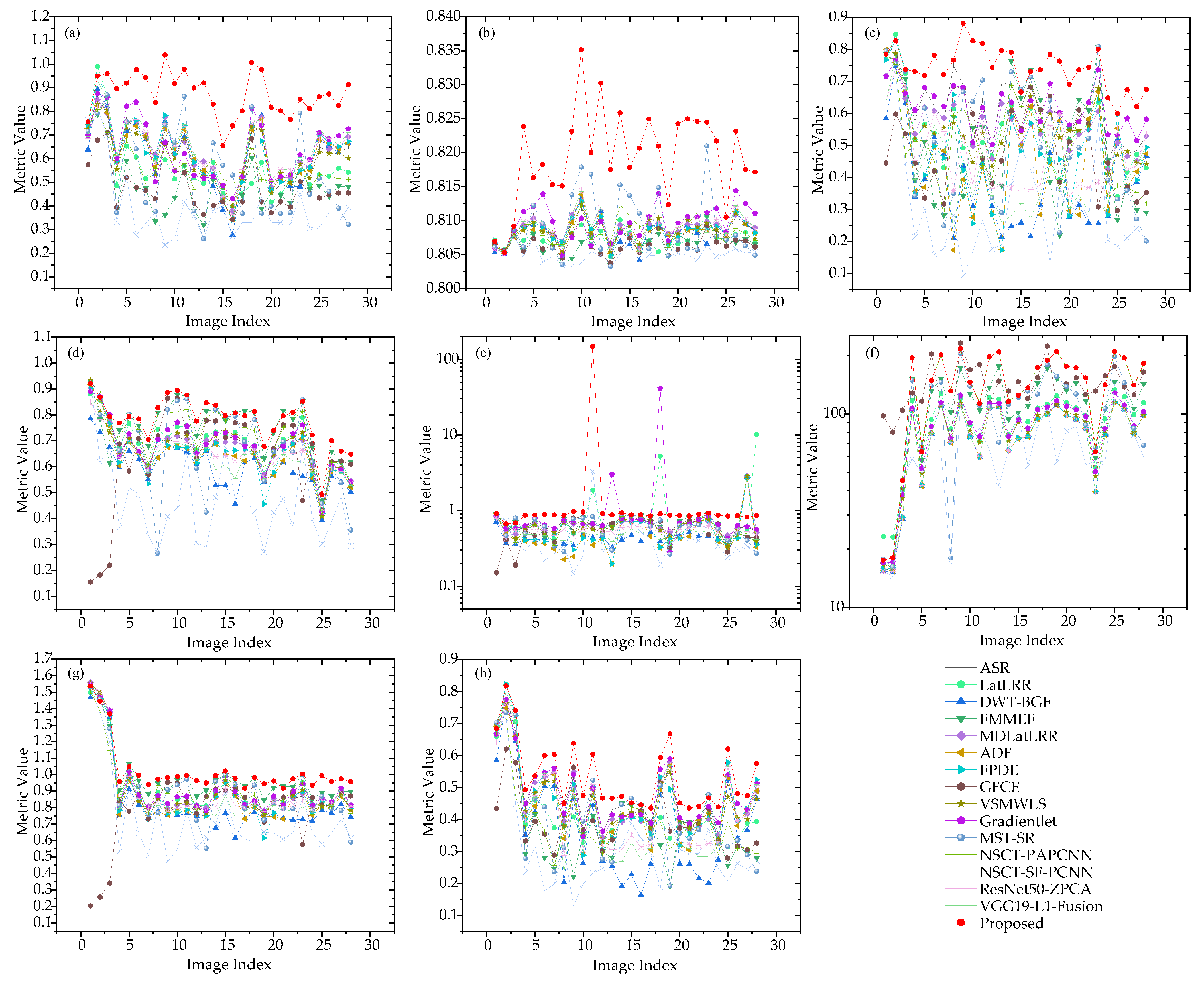
To further demonstrate the effectiveness of each part of the algorithm, we selected four metrics to assess the final fusion results. These metrics are MI, NCIE, $Q_{ab/f}$, and SSIM. The experimental results are shown in

Table 5. Objective values of different structure methods. The best metric values are in bold.

Methods	MI	NCIE	${\mathit{Q}}_{\mathbf{ab}/\mathit{f}}$	SSIM
MLSW + SP + SL	0.7711	0.8206	0.6411	0.8875
AMLSW + SP	0.7946	0.8222	0.6827	0.9489
AMLSW + SL	0.7709	0.8206	0.6413	0.8874
AMLSW + SP + SL	0.8061	0.8230	0.6794	0.9523

, where the best metric values have been bolded.

In Table 5, we can draw the same conclusion as above: (1) The asymmetric decomposition structure has better fusion performance compared with the symmetric decomposition structure by comparing the metrics of MLSW + SP + SL and AMLSW + SP + SL. (2) The SF-LV fusion strategy has a better performance in detail preservation by comparing the metrics of AMLSW + SP and AMLSW + SP + SL. (3) The SPhCM-PCNN fusion strategy has a better performance in edge preservation by comparing the metrics of AMLSW + SL and AMLSW + SP + SL. We can find that all of the structures are necessary for good fusion performance.

As analyzed above, both in the objective and subjective evaluations, the asymmetric structure proposed in this method performs better than the symmetric one. This is because the asymmetric structure extracts more weak signals and effectively enhances them. The fusion strategies can also effectively preserve the details according to the characteristics of the corresponding layers. The main structures proposed in this study are both necessary and effective. The proposed method can inspire researchers to consider a new asymmetric fusion framework that can adapt to the differences in information richness of the images, and promote the development of fusion technology.

4.3. Generalization Analysis of the Method

To validate the adaptability and applicability of our proposed method on real-world data, we discuss the applicability of the proposed method in this section. We use publicly available infrared and visible fusion datasets to validate the proposed method. The infrared and visible fusion datasets that are widely used by many researchers include TNO [64], RoadScene [33], Multi-Spectral Road Scenarios(MSRS) [65], etc.

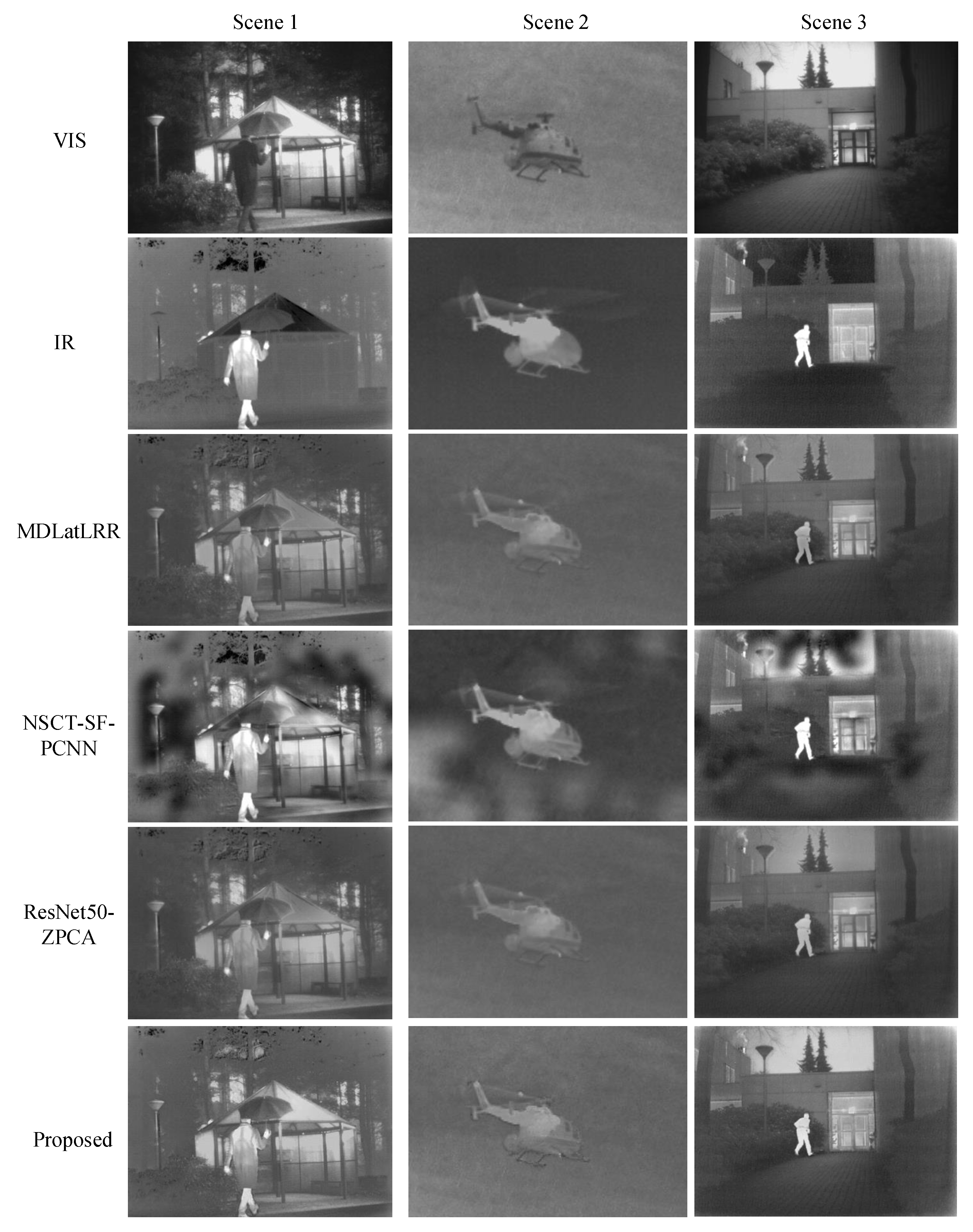
For the evaluation carried out in this study, we used the TNO datasets for infrared and visible image fusion. The TNO dataset contains images captured in various bands, including visual (390–700 nm), near-infrared (700–1000 nm), and longwave-infrared (8–12 $\mathsf{\mu }$m). The scenarios were captured at nighttime so that the advantage of infrared could be exploited. All of the images are registered at the pixel level with different multi-band camera systems.

To illustrate the performance of our method, we compared it with three other infrared and visible image fusion methods: MDLatLRR, NSCT-SF-PCNN and ResNet50-ZPCA. The fusion results are shown in Figure 14.

Through the results shown in Figure 14, we find that our proposed method can also be applied to infrared and visible image fusion. Due to the fact that infrared and visible light images are obtained from different types of signal sources, there is a relatively large information difference. The proposed method can deal with two different images with large information differences. Therefore, our method is also suitable for fusing infrared and visible images. The image data used for fusion are all from real scenes, which indicates that our method is capable of processing the image information of real scenes with information differences.

To further demonstrate the applicability of our method, we used four fusion metrics to evaluate the fusion performance: MI, NCIE, $Q_{ab/f}$, and $Q_Y$. The metric values of different fusion methods in different scenes are shown in

Table 6. Objective value comparison of different methods in different scenes. The best metric values are in bold.

	Methods	MI	NCIE	${\mathit{Q}}_{\mathbf{ab}/\mathit{f}}$	${\mathit{Q}}_{\mathit{Y}}$
Scene 1	MDLatLRR	0.3062	0.8042	0.3988	0.7311
	NSCT-SF-PCNN	0.2440	0.8035	0.3919	0.7521
	ResNet50-ZPCA	0.3023	0.8043	0.3590	0.6963
	Proposed	0.3546	0.8047	0.4077	0.7398
Scene 2	MDLatLRR	0.4423	0.8044	0.4133	0.7804
	NSCT-SF-PCNN	0.2872	0.8034	0.2777	0.6541
	ResNet50-ZPCA	0.4338	0.8042	0.3442	0.7124
	Proposed	0.5098	0.8062	0.4373	0.8115
Scene 3	MDLatLRR	0.3199	0.8044	0.3886	0.7135
	NSCT-SF-PCNN	0.3400	0.8059	0.5488	0.8798
	ResNet50-ZPCA	0.3122	0.8044	0.3444	0.6785
	Proposed	0.4061	0.8060	0.3872	0.7229

, where the best values have been bolded.

As is evident in Table 6, the proposed method achieves the best values for these four metrics. Hence, in view of objective metrics, the proposed method is applicable to the task of infrared and visible image fusion. Our proposed method exhibits good adaptability.

4.4. Analysis of Time Complexity

Because the proposed fusion method has a relatively complex structure, it is necessary to conduct a time complexity analysis of the method. In this part, we analyze the time consumption for the proposed method.

The time complexity analysis can be performed by analyzing the number of operations required to complete the method as a function of the input size. The time complexity of the method is typically denoted as $O\left(f\right(n\left)\right)$, where n represents the input size.

In our study, the entire processing procedure can be divided into four stages: image complexity assessment, image decomposition, multi-level image fusion, and the aggregation process. Suppose that the size of the input image is $n=M\times N$. For the image complexity assessment stage, the SF and the variance are calculated. Both the SF and the variance have an $O\left(n\right)$ complexity. Thus, the time complexity of this stage is $O\left(MN\right)$. For the image decomposition stage, the MLSW and MLSW-GS are adopted. MLSW-GS has a higher complexity than MLSW. The complexity of MLSW-GS is determined by the number of decomposition layers s, filter operation, and guided operation. The complexity of the filter operation is determined by the kernel size k. It has an $O\left(n{k}^2\right)$ complexity, and so is the guided operation. So in this stage, the time complexity is $O\left(2sMN{k}^2\right)$. For the multi-level image fusion stage, SPhCM-PCNN, SF-LV and Energy based fusion strategies are adopted. Both SF-LV and Energy-based method have $O\left(n\right)$ complexity. The time complexity of SPhCM-PCNN is $O\left(MN(4llog\left(MN\right)+C_{cof}+L)\right)$, where the l is the scale parameter in SPhC method. The 4 represents the four orientations in SPhC. $C_{cof}=\frac{1}{3}(t+1)(4{(t+1)}^2-1)-1$. t is the number of scales in SPhCM. L is the iteration number in PCNN. So in this stage, the time complexity is $O\left(MN(4llog\left(MN\right)+C_{cof}+L)\right)$. For the aggregating process stage, a sum operation is adopted. Sum operation has an $O\left(n\right)$ complexity. So in this stage, the complexity is determined by the number of decomposition layers s. The time complexity of this stage is $O\left(sMN\right)$. Hence, the time complexity of the entire proposed method is $O\left(MN(s+1+2s{k}^2+4llog\left(MN\right)+C_{cof}+L)\right)$. As we analyzed, the second and third stages account for the main part of the time consumption of the proposed method.

To demonstrate the run-time of the proposed method more specifically, we separately timed each stage of the method. The results are shown in

Table 7. Time consumption of different stages in the proposed method. Stage 1 is image complexity assessment. Stage 2 is image decomposition. Stage 3 is multi-level image fusion. Stage 4 is the aggregation process.

Stage 1	Stage 2	Stage 3	Stage 4	Total
0.0037	0.1052	1.5114	0.0008	1.6211

. It should be noted that the input image size is $151\times 151$.

The results in Table 7 indicate that the time consumption of the proposed method is mainly concentrated in the image decomposition and multi-level image fusion stages, which is consistent with our previous analysis of time complexity.

To compare the time consumption with other state-of-the-art methods, we selected four of the methods mentioned above as references, timed them, and compared the results. The experimental results are shown in

Table 8. Time consumption of different methods. The best metric values are in bold.

Methods	ASR	LatLRR	ADF	FMMEF	Proposed
Time	14.9868	3.3599	0.0440	0.0870	1.6211

.

Compared with other methods, our method has a higher time complexity and longer processing time. It can not meet the real-time processing requirement. This needs further improvement to help our proposed method enter engineering practice. One feasible solution is to design a parallel structure for the method because the main structures of the method process the images in the local area, which is more amenable to parallel computation. Furthermore, simplification methods for some structures can also be used to improve the time performance.

5. Conclusions

In this work, a novel fusion method named adaptive guided multi-layer side window box filter decomposition (AMLSW-GS) is proposed to mitigate detail loss in the fusion process of ISAR and visible images. Firstly, a new information abundance discrimination method based on spatial frequency and variance is proposed to sort the input images into detailed and coarse images. Secondly, the MLSW decomposition and MLSW-GS decomposition methods are proposed to decompose the detailed image and the coarse image into different scales, respectively. Thirdly, four fusion strategies—sum fusion, SF-LV, SPhCM-PCNN, and energy-based methods—are adopted to fuse different scale features to retain more detail. Finally, the fusion result is obtained by accumulating different sub-fusion results. In this way, the proposed method can make full use of the latent features from different types of images and retain more detail in the fusion result. On the synthetic ISAR-VIS dataset and the real-world IR-VIS dataset, compared with other state-of-the-art fusion methods, the experimental results show that the proposed method has the best performance in both subjective and objective fusion quality evaluations. This demonstrates the superiority and effectiveness of the proposed asymmetric decomposition methods.

Additionally, the unstable parameters limit the overall performance of the method, and further optimization is needed for the weak signal enhancement method. Simultaneously, the fusion time is in the order of seconds, which cannot meet the real-time requirements of engineering. In the future, we will mainly research more effective methods of enhancing weak signals to better preserve information. Furthermore, we will consider the execution efficiency of the methods while designing fusion strategies to make them applicable in engineering practices.

References

1. Yi, S.; Jiang, G.; Liu, X.; Li, J.; Chen, L. TCPMFNet: An infrared and visible image fusion network with composite auto encoder and transformer–convolutional parallel mixed fusion strategy. Infrared Phys. Technol. 2022, 127, 104405. [Google Scholar] [CrossRef]
2. Huang, Z.; Yang, B.; Liu, C. RDCa-Net: Residual dense channel attention symmetric network for infrared and visible image fusion. Infrared Phys. Technol. 2023, 130, 104589. [Google Scholar] [CrossRef]
3. Zhang, X.; Liu, G.; Huang, L.; Ren, Q.; Bavirisetti, D.P. IVOMFuse: An image fusion method based on infrared-to-visible object mapping. Digit. Signal Process. 2023, 137, 104032. [Google Scholar] [CrossRef]
4. Liu, X.; Wang, R.; Huo, H.; Yang, X.; Li, J. An attention-guided and wavelet-constrained generative adversarial network for infrared and visible image fusion. Infrared Phys. Technol. 2023, 129, 104570. [Google Scholar] [CrossRef]
5. Tan, W.; Zhou, H.; Rong, S.; Qian, K.; Yu, Y. Fusion of multi-focus images via a Gaussian curvature filter and synthetic focusing degree criterion. Appl. Opt. 2018, 57, 10092–10101. [Google Scholar] [CrossRef]
6. Su, W.; Huang, Y.; Li, Q.; Zuo, F. GeFuNet: A knowledge-guided deep network for the infrared and visible image fusion. Infrared Phys. Technol. 2022, 127, 104417. [Google Scholar] [CrossRef]
7. Liu, Y.; Chen, X.; Cheng, J.; Peng, H.; Wang, Z. Infrared and visible image fusion with convolutional neural networks. Int. J. Wavelets Multiresolut. Inf. Process. 2018, 16, 1850018. [Google Scholar] [CrossRef]
8. Zhuang, D.; Zhang, L.; Zou, B. An Interferogram Re-Flattening Method for InSAR Based on Local Residual Fringe Removal and Adaptively Adjusted Windows. Remote Sens. 2023, 15, 2214. [Google Scholar] [CrossRef]
9. Shao, Z.; Zhang, T.; Ke, X. A Dual-Polarization Information-Guided Network for SAR Ship Classification. Remote Sens. 2023, 15, 2138. [Google Scholar] [CrossRef]
10. Byun, Y.; Choi, J.; Han, Y. An area-based image fusion scheme for the integration of SAR and optical satellite imagery. IEEE J. Sel. Top. Appl. Earth Obs. Remote Sens. 2013, 6, 2212–2220. [Google Scholar] [CrossRef]
11. Iervolino, P.; Guida, R.; Riccio, D.; Rea, R. A novel multispectral, panchromatic and SAR data fusion for land classification. IEEE J. Sel. Top. Appl. Earth Obs. Remote Sens. 2019, 12, 3966–3979. [Google Scholar] [CrossRef]
12. Li, B.; Xian, Y.; Zhang, D.; Su, J.; Hu, X.; Guo, W. Multi-sensor image fusion: A survey of the state of the art. J. Comput. Commun. 2021, 9, 73–108. [Google Scholar] [CrossRef]
13. Li, S.; Kwok, J.T.; Wang, Y. Combination of images with diverse focuses using the spatial frequency. Inf. Fusion 2001, 2, 169–176. [Google Scholar] [CrossRef]
14. Mitianoudis, N.; Stathaki, T. Pixel-based and region-based image fusion schemes using ICA bases. Inf. Fusion 2007, 8, 131–142. [Google Scholar] [CrossRef]
15. Li, X.; Wang, L.; Wang, J.; Zhang, X. Multi-focus image fusion algorithm based on multilevel morphological component analysis and support vector machine. IET Image Process. 2017, 11, 919–926. [Google Scholar] [CrossRef]
16. Li, H.; Wu, X.J. Infrared and visible image fusion using latent low-rank representation. arXiv 2018, arXiv:1804.08992. [Google Scholar]
17. Liu, Y.; Wang, Z. Simultaneous image fusion and denoising with adaptive sparse representation. IET Image Process. 2015, 9, 347–357. [Google Scholar] [CrossRef]
18. Yin, M.; Liu, X.; Liu, Y.; Chen, X. Medical image fusion with parameter-adaptive pulse coupled neural network in nonsubsampled shearlet transform domain. IEEE Trans. Instrum. Meas. 2018, 68, 49–64. [Google Scholar] [CrossRef]
19. Li, H.; Wu, X.J.; Kittler, J. Infrared and visible image fusion using a deep learning framework. In Proceedings of the 2018 24th International Conference on Pattern Recognition (ICPR), Beijing, China, 20–24 August 2018; pp. 2705–2710. [Google Scholar]
20. Tan, W.; Tiwari, P.; Pandey, H.M.; Moreira, C.; Jaiswal, A.K. Multimodal medical image fusion algorithm in the era of big data. Neural Comput. Appl. 2020, 2020, 1–21. [Google Scholar] [CrossRef]
21. Zhang, S.; Li, X.; Zhang, X.; Zhang, S. Infrared and visible image fusion based on saliency detection and two-scale transform decomposition. Infrared Phys. Technol. 2021, 114, 103626. [Google Scholar] [CrossRef]
22. Wan, T.; Zhu, C.; Qin, Z. Multifocus image fusion based on robust principal component analysis. Pattern Recognit. Lett. 2013, 34, 1001–1008. [Google Scholar] [CrossRef]
23. Yang, Y.; Zhang, W.; Huang, S.; Wan, W.; Liu, J.; Kong, X. Infrared and visible image fusion based on dual-kernel side window filtering and S-shaped curve transformation. IEEE Trans. Instrum. Meas. 2021, 71, 1–15. [Google Scholar] [CrossRef]
24. Smadi, A.A.; Abugabah, A.; Mehmood, A.; Yang, S. Brain image fusion approach based on side window filtering. Procedia Comput. Sci. 2022, 198, 295–300. [Google Scholar] [CrossRef]
25. Yan, H.; Zhang, J.X.; Zhang, X. Injected Infrared and Visible Image Fusion via L_{1} Decomposition Model and Guided Filtering. IEEE Trans. Comput. Imaging 2022, 8, 162–173. [Google Scholar] [CrossRef]
26. Zou, D.; Yang, B. Infrared and low-light visible image fusion based on hybrid multiscale decomposition and adaptive light adjustment. Opt. Lasers Eng. 2023, 160, 107268. [Google Scholar] [CrossRef]
27. Liu, Y.; Liu, S.; Wang, Z. A general framework for image fusion based on multi-scale transform and sparse representation. Inf. Fusion 2015, 24, 147–164. [Google Scholar] [CrossRef]
28. Zhang, Q.; Levine, M.D. Robust multi-focus image fusion using multi-task sparse representation and spatial context. IEEE Trans. Image Process. 2016, 25, 2045–2058. [Google Scholar] [CrossRef]
29. Liu, X.; Mei, W.; Du, H. Structure tensor and nonsubsampled shearlet transform based algorithm for CT and MRI image fusion. Neurocomputing 2017, 235, 131–139. [Google Scholar] [CrossRef]
30. Qu, X.B.; Yan, J.W.; Hong-Zhi, X.; Zi-Qian, Z. Image fusion algorithm based on spatial frequency-motivated pulse coupled neural networks in nonsubsampled contourlet transform domain. Acta Autom. Sin. 2008, 34, 1508–1514. [Google Scholar] [CrossRef]
31. Panigrahy, C.; Seal, A.; Mahato, N.K. MRI and SPECT image fusion using a weighted parameter adaptive dual channel PCNN. IEEE Signal Process. Lett. 2020, 27, 690–694. [Google Scholar] [CrossRef]
32. Indhumathi, R.; Narmadha, T. Hybrid pixel based method for multimodal image fusion based on Integration of Pulse Coupled Neural Network (PCNN) and Genetic Algorithm (GA) using Empirical Mode Decomposition (EMD). Microprocess. Microsyst. 2022, 94, 104665. [Google Scholar] [CrossRef]
33. Xu, H.; Ma, J.; Jiang, J.; Guo, X.; Ling, H. U2Fusion: A unified unsupervised image fusion network. IEEE Trans. Pattern Anal. Mach. Intell. 2022, 44, 502–518. [Google Scholar] [CrossRef] [PubMed]
34. Li, H.; Wu, X.J. DenseFuse: A fusion approach to infrared and visible images. IEEE Trans. Image Process. 2018, 28, 2614–2623. [Google Scholar] [CrossRef] [PubMed]
35. Ma, J.; Yu, W.; Liang, P.; Li, C.; Jiang, J. FusionGAN: A generative adversarial network for infrared and visible image fusion. Inf. Fusion 2019, 48, 11–26. [Google Scholar] [CrossRef]
36. Xu, H.; Ma, J.; Zhang, X.P. MEF-GAN: Multi-exposure image fusion via generative adversarial networks. IEEE Trans. Image Process. 2020, 29, 7203–7216. [Google Scholar] [CrossRef]
37. Yin, H.; Gong, Y.; Qiu, G. Side window filtering. In Proceedings of the IEEE/CVF Conference on Computer Vision and Pattern Recognition, Long Beach, CA, USA, 15–20 June 2019; pp. 8758–8766. [Google Scholar]
38. He, K.; Sun, J.; Tang, X. Guided Image Filtering. In Proceedings of the European Conference on Computer Vision, Heraklion, Greece, 5–11 September 2010. [Google Scholar]
39. Kovesi, P. Image features from phase congruency. Videre: J. Comput. Vis. Res. 1999, 1, 1–26. [Google Scholar]
40. Morrone, M.C.; Owens, R.A. Feature detection from local energy. Pattern Recognit. Lett. 1987, 6, 303–313. [Google Scholar] [CrossRef]
41. Kovesi, P. Symmetry and asymmetry from local phase. In Proceedings of the Tenth Australian Joint Conference on Artificial Intelligence, Perth, Australia, 30 November–4 December 1997; Volume 190, pp. 2–4. [Google Scholar]
42. Xiao, Z.; Hou, Z.; Guo, C. Image feature detection technique based on phase information: Symmetry phase congruency. J. Tianjin Univ. 2004, 37, 695–699. [Google Scholar]
43. Zhang, F.; Zhang, B.; Zhang, R.; Zhang, X. SPCM: Image quality assessment based on symmetry phase congruency. Appl. Soft Comput. 2020, 87, 105987. [Google Scholar] [CrossRef]
44. Johnson, J.L.; Padgett, M.L. PCNN Models and Applications. IEEE Trans. Neural Netw. 1999, 10, 480–498. [Google Scholar] [CrossRef]
45. Teng, X. VisableAerial-Target. Available online: https://github.com/TengXiang164/VisableAerial-Target (accessed on 4 April 2023).
46. Richards, M.A. Fundamentals of Radar Signal Processing; McGraw-Hill Education: New York, NY, USA, 2014. [Google Scholar]
47. Li, H.; Wu, X.J.; Kittler, J. MDLatLRR: A novel decomposition method for infrared and visible image fusion. IEEE Trans. Image Process. 2020, 29, 4733–4746. [Google Scholar] [CrossRef] [PubMed]
48. Zhang, X.; Ye, P.; Xiao, G. VIFB: A visible and infrared image fusion benchmark. In Proceedings of the IEEE/CVF Conference on Computer Vision and Pattern Recognition Workshops, Seattle, WA, USA, 14–19 June 2020; pp. 104–105. [Google Scholar]
49. Bavirisetti, D.P.; Dhuli, R. Fusion of infrared and visible sensor images based on anisotropic diffusion and Karhunen-Loeve transform. IEEE Sens. J. 2015, 16, 203–209. [Google Scholar] [CrossRef]
50. Bavirisetti, D.P.; Xiao, G.; Liu, G. Multi-sensor image fusion based on fourth order partial differential equations. In Proceedings of the IEEE 2017 20th International Conference on Information Fusion (Fusion), Xi’an, China, 10–13 July 2017; pp. 1–9. [Google Scholar]
51. Li, H.; Ma, K.; Yong, H.; Zhang, L. Fast multi-scale structural patch decomposition for multi-exposure image fusion. IEEE Trans. Image Process. 2020, 29, 5805–5816. [Google Scholar] [CrossRef] [PubMed]
52. Zhou, Z.; Dong, M.; Xie, X.; Gao, Z. Fusion of infrared and visible images for night-vision context enhancement. Appl. Opt. 2016, 55, 6480–6490. [Google Scholar] [CrossRef] [PubMed]
53. Ma, J.; Zhou, Z.; Wang, B.; Zong, H. Infrared and visible image fusion based on visual saliency map and weighted least square optimization. Infrared Phys. Technol. 2017, 82, 8–17. [Google Scholar] [CrossRef]
54. Ma, J.; Zhou, Y. Infrared and visible image fusion via gradientlet filter. Comput. Vis. Image Underst. 2020, 197, 103016. [Google Scholar] [CrossRef]
55. Biswas, B. Guided-Bilateral Filter-Based Medical Image Fusion Using Visual Saliency Map in the Wavelet Domain. Available online: https://github.com/biswajitcsecu/Guided-Bilateral-Filter-based-Medical-Image-Fusion-Using-Visual-Saliency-Map-in-the-Wavelet-Domain (accessed on 4 April 2023).
56. Li, H.; Wu, X.J.; Durrani, T.S. Infrared and Visible Image Fusion with ResNet and zero-phase component analysis. Infrared Phys. Technol. 2019, 102, 103039. [Google Scholar] [CrossRef]
57. Cvejic, N.; Canagarajah, C.; Bull, D. Image fusion metric based on mutual information and Tsallis entropy. Electron. Lett. 2006, 42, 1. [Google Scholar] [CrossRef]
58. Wang, Q.; Shen, Y.; Jin, J. Performance evaluation of image fusion techniques. Image Fusion Algorithms Appl. 2008, 19, 469–492. [Google Scholar]
59. Xydeas, C.S.; Petrovic, V.S. Objective pixel-level image fusion performance measure. In Proceedings of the Sensor Fusion: Architectures, Algorithms, and Applications IV, SPIE, Orlando, FL, USA, 6–7 April 2000; Volume 4051, pp. 89–98. [Google Scholar]
60. Piella, G.; Heijmans, H. A new quality metric for image fusion. In Proceedings of the IEEE 2003 International Conference on Image Processing (Cat. No. 03CH37429), Barcelona, Spain, 14–17 September 2003; Volume 3, pp. 3–173. [Google Scholar]
61. Li, S.; Hong, R.; Wu, X. A novel similarity based quality metric for image fusion. In Proceedings of the IEEE 2008 International Conference on Audio, Language and Image Processing, Shanghai, China, 7–9 July 2008; pp. 167–172. [Google Scholar]
62. Haghighat, M.B.A.; Aghagolzadeh, A.; Seyedarabi, H. A non-reference image fusion metric based on mutual information of image features. Comput. Electr. Eng. 2011, 37, 744–756. [Google Scholar] [CrossRef]
63. Haghighat, M.; Razian, M.A. Fast-FMI: Non-reference image fusion metric. In Proceedings of the 2014 IEEE 8th International Conference on Application of Information and Communication Technologies (AICT), Astana, Kazakhstan, 15–17 October 2014; pp. 1–3. [Google Scholar]
64. Toet, A. The TNO multiband image data collection. Data Brief 2017, 15, 249–251. [Google Scholar] [CrossRef] [PubMed]
65. Ma, J.; Tang, L.; Fan, F.; Huang, J.; Mei, X.; Ma, Y. SwinFusion: Cross-domain Long-range Learning for General Image Fusion via Swin Transformer. IEEE/CAA J. Autom. Sin. 2022, 9, 1200–1217. [Google Scholar] [CrossRef]
Figure 1. Framework of the proposed method.
Remotesensing 15 02784 g001
Figure 2. Framework of MLSW.
Remotesensing 15 02784 g002
Figure 3. Framework of the MLSW-GS.
Remotesensing 15 02784 g003
Figure 4. Framework of the SPhCM-PCNN.
Remotesensing 15 02784 g004
Figure 5. Some samples in the public dataset.
Remotesensing 15 02784 g005
Figure 6. Results of different fusion methods in scene 1. The red box shows the detail preservation of ISAR, magnified in the upper right corner, while the green box demonstrates the information preservation of the visible image, mainly in terms of signal intensity. They are listed as follows: (a) Source of VIS. (b) Source of ISAR. (c) Result of ASR. (d) Result of MDLatLRR. (e) Result of ADF. (f) Result of FPDE. (g) Result of FMMEF. (h) Result of GFCE. (i) Result of VSMWLS. (j) Result of Gradientlet. (k) Result of LatLRR. (l) Result of NSCT-PAPCNN. (m) Result of NSCT-SF-PCNN. (n) Result of MST-SR. (o) Result of DWT-BGF. (p) Result of VGG19-L1-Fusion. (q) Result of ResNet50-ZPCA. (r) Result of the proposed method.
Remotesensing 15 02784 g006
Figure 7. Results of different fusion methods in scene 2. The red box shows the detail preservation of ISAR, magnified in the upper right corner, while the green box demonstrates the information preservation of the visible image, mainly in terms of signal intensity. They are listed as follows: (a) Source of VIS. (b) Source of ISAR. (c) Result of ASR. (d) Result of MDLatLRR. (e) Result of ADF. (f) Result of FPDE. (g) Result of FMMEF. (h) Result of GFCE. (i) Result of VSMWLS. (j) Result of Gradientlet. (k) Result of LatLRR. (l) Result of NSCT-PAPCNN. (m) Result of NSCT-SF-PCNN. (n) Result of MST-SR. (o) Result of DWT-BGF. (p) Result of VGG19-L1-Fusion. (q) Result of ResNet50-ZPCA. (r) Result of the proposed method.
Remotesensing 15 02784 g007
Figure 8. Different results of different fusion methods in scene 3. The red box shows the detail preservation of ISAR, magnified in the upper right corner, while the green box demonstrates the information preservation of the visible image, mainly in terms of signal intensity. They are listed as follows: (a) Source of VIS. (b) Source of ISAR. (c) Result of ASR. (d) Result of MDLatLRR. (e) Result of ADF. (f) Result of FPDE. (g) Result of FMMEF. (h) Result of GFCE. (i) Result of VSMWLS. (j) Result of Gradientlet. (k) Result of LatLRR. (l) Result of NSCT-PAPCNN. (m) Result of NSCT-SF-PCNN. (n) Result of MST-SR. (o) Result of DWT-BGF. (p) Result of VGG19-L1-Fusion. (q) Result of ResNet50-ZPCA. (r) Result of the proposed method.
Remotesensing 15 02784 g008
Figure 9. Results of different fusion methods in scene 4. The red box shows the detail preservation of ISAR, magnified in the upper right corner, while the green box demonstrates the information preservation of the visible image, mainly in terms of signal intensity. They are listed as follows: (a) Source of VIS. (b) Source of ISAR. (c) Result of ASR. (d) Result of MDLatLRR. (e) Result of ADF. (f) Result of FPDE. (g) Result of FMMEF. (h) Result of GFCE. (i) Result of VSMWLS. (j) Result of Gradientlet. (k) Result of LatLRR. (l) Result of NSCT-PAPCNN. (m) Result of NSCT-SF-PCNN. (n) Result of MST-SR. (o) Result of DWT-BGF. (p) Result of VGG19-L1-Fusion. (q) Result of ResNet50-ZPCA. (r) Result of the proposed method.
Remotesensing 15 02784 g009
Figure 10. Comparison of different methods used on representative scenes. (a) MI values of Different Methods (b) NICE values of Different Methods (c) Q a b / f values of Different Methods (d) Q S values of Different Methods (e) Q Y values of Different Methods (f) Average values of Different Methods (g) SSIM values of Different Methods (h) FMI values of Different Methods.
Remotesensing 15 02784 g010
Figure 11. Performance under different numbers of decompositions. (a) is the result of MI, and (b) is the result of Q a b / f . In this experiment, the number of scales in morphological operation t is 3.
Remotesensing 15 02784 g011
Figure 12. Performance under different numbers of scales. (a) is the result of MI, and (b) is the result of Q a b / f . In this experiment, the number of decompositions s is 3.
Remotesensing 15 02784 g012
Figure 13. Comparison of results of different model structures. (a) is the Source of VIS, (b) is the Source of ISAR, (c) AMLSW + SP + SL, (d) MLSW + SP + SL, (e) AMLSW + SP, (f) AMLSW + SL, (g) Difference between AMLSW + SP + SL and AMLSW + SP + SL, (h) Difference between MLSW + SP + SL and AMLSW + SP + SL, (i) Difference between AMLSW + SP and AMLSW + SP + SL, (j) Difference between AMLSW + SL and AMLSW + SP + SL.
Remotesensing 15 02784 g013
Figure 14. Results of different methods for infrared and visible image fusion. Different scenes are shown in different columns. The first row contains the visible images, the second row contains the infrared images, the third row contains the fusion results of MDLatLRR, the fourth row contains the fusion results of NSCT-SF-PCNN, the fifth row contains the fusion results of ResNet50-ZPCA, and the last row contains the fusion results of the proposed method.
Remotesensing 15 02784 g014