Changes in Carbon Dioxide Balance Associated with Land Use and Land Cover in Brazilian Legal Amazon Based on Remotely Sensed Imagery

Abstract

The Amazon region comprises the largest tropical forest on the planet and is responsible for absorbing huge amounts of CO₂ from the atmosphere. However, changes in land use and cover have contributed to an increase in greenhouse gas emissions, especially CO₂, and in endangered indigenous lands and protected areas in the region. The objective of this study was to detect changes in CO₂ emissions and removals associated with land use and land cover changes in the Brazilian Legal Amazon (BLA) through the analysis of multispectral satellite images from 2009 to 2019. The Gross Primary Production (GPP) and CO₂Flux variables were estimated by the MODIS sensor onboard Terra and Aqua satellite, representing carbon absorption by vegetation during the photosynthesis process. Atmospheric CO₂ concentration was estimated from the GOSAT satellite. The variables GPP and CO₂Flux showed the effective flux of carbon in the BLA to atmosphere, which were weakly correlated with precipitation (r = 0.191 and 0.133). The forest absorbed 211.05 TgC annually but, due to its partial conversion to other land uses, the loss of 135,922.34 km² of forest area resulted in 5.82 TgC less carbon being absorbed. Pasture and agriculture, which comprise the main land conversions, increased by 100,340.39 km² and absorbed 1.32 and 3.19 TgC less, and emitted close to twice more, than forest in these areas. Atmospheric CO₂ concentrations increased from 2.2 to 2.8 ppm annually in BLA, with hotspots observed in the southeast Amazonia, and CO₂ capture by GPP showed an increase over the years, mainly after 2013, in the north and west of the BLA. This study brings to light the carbon dynamics, by GPP and CO₂Flux models, as related to the land use and land cover in one of the biggest world carbon reservoirs, the Amazon, which is also important to fulfillment of international agreements signed by Brazil to reduce greenhouse gas emissions and for biodiversity conservation and other ecosystem services in the region.

1. Introduction

Intact forest ecosystems play a key role in increasing resilience to climate change, and conserving biodiversity [1,2]. The Brazilian Legal Amazon, delimited according to Art. 2 of Complementary Law No. 124, of 3 January 2007 [3], has a total area of 5.02 M km², corresponding to 58.9% of the Brazilian territory [4]. This area is responsible for holding the Earth’s greatest biodiversity and above ground biomass, also accounting for one of the largest sources of mineral and biological resources [5,6,7].

Among the ecosystem services provided is the removal of carbon through CO₂ from the atmosphere, via capture and storage by increase in gross primary production (GPP) [8,9,10]. A total forest sink of 2.4 ± 0.4 Pg C year⁻¹ was estimated globally, and 262.1 Pg C of this was stocked in tropical America [11]. The GPP relates to carbon dioxide absorption during the photosynthesis process [12,13,14]. The analysis of anomalies in the GPP values determines the impact of changes in both carbon absorption and emissions [15]. It is possible and necessary to accurately estimate their temporal and spatial variations to understand several ecosystem functions in response to climate and land use and land cover changes [16,17]. These processes play an important role in the carbon balance between the atmosphere and the biosphere [6,18], as well as in the modifications in response to climate change [19,20,21]. These modifications are mainly related to forest loss, induced by deforestation, which contributes to greenhouse gas emissions, thus worsening global warming [22,23,24].

Indigenous lands (IL), areas destined for the indigenous population, and protected areas (PA), areas for environmental conservation, in the BLA accounted for 43% of the total land area and covered about half of the total forest area in the region [2]; they are important in conserving the standing forest, biodiversity, and in mitigating the climate in the Brazilian Legal Amazon, as they act as “shields” against deforestation [2,25,26]. However, forest conservation in IL/PA has been facing increasing threats from weak environmental laws and regulations, changes in government priorities and massive economic development [24,27,28]. In the Brazilian Legal Amazon (BLA), 75% of deforestation has occurred in large swathes along highways, most of them close to Ils and Pas, inducing forest losses due to different land use and land cover changes [28,29]. An example is the paving of the Belém-Brasília (BR-010) and Cuiabá-Porto Velho (BR-364) highways that originated the so-called “arc of deforestation” [30,31].

Increased carbon emissions, land use and land cover changes, and anthropogenic pressure are the main drivers in the degradation of tropical forests, such as the Amazon, which have led to severe losses of carbon sinks [22,32,33]. Land use and land cover changes caused by anthropogenic activities have substantially altered carbon cycling, contributing to the increase in atmospheric CO₂ concentration (XCO₂), among other greenhouse gases, which is the main cause of global warming and climate change [34]. Land use change in tropical climates accounted for 1.1 ± 0.7 Pg C of terrestrial carbon emissions between 2000–2007 [11]. The historical assessment of land use and land cover changes is important for the management of natural resources and the development of sustainable policies, as it gives insights into the interaction between the environment and humans in a given region, thus preventing further environmental degradation in several aspects [35,36,37].

Remote sensing techniques are often used to better understand land use and land cover changes, as they reduce the cost and time necessary to detect environmental degradation [38,39,40] and climate and carbon fluxes, as extensively covered in the recent literature [18,20,21,34,41,42,43]. Remote sensing has recently been applied to updating the boundaries between the Brazilian Cerrado-Amazon biomes, due to land use and land cover changes, by using vegetation indices such as Gross Primary Productivity (GPP) and carbon dioxide fluxes (CO₂Flux), allowing the development of public policies to curb deforestation and degradation by anthropogenic activities [44]. Remote sensing has also been crucial in helping to uncover the vital role and substantial progress made by IL and PA in conserving the Amazon, and the risks from the recent weakening of forest policies in Brazil [2,45].

Studies point out that 40% deforestation in the Amazon would lead to a decrease in rainfall and a longer dry season. They also highlight that 20–25% deforestation would be the tipping point for the Amazonian system to shift to a non-forest ecosystem in most of the Amazon [35,36,46,47]. In this regard, it is expected that changes in CO₂ emissions and removals induced by land use and land cover changes in the Brazilian Legal Amazon have intensified in recent years and could be identified and quantified through MODIS images and physically based models. Here, we investigate the relationship between land use and land cover changes, GPP, CO₂Flux, XCO₂ and precipitation in the Brazilian Legal Amazon from 2009 to 2019. We believe that the investigation into the loss or gain in the carbon absorption capacity of these areas could facilitate more environmentally friendly and sustainable decisions, in order to preserve BLA and carbon pools in the region.

2. Materials and Methods

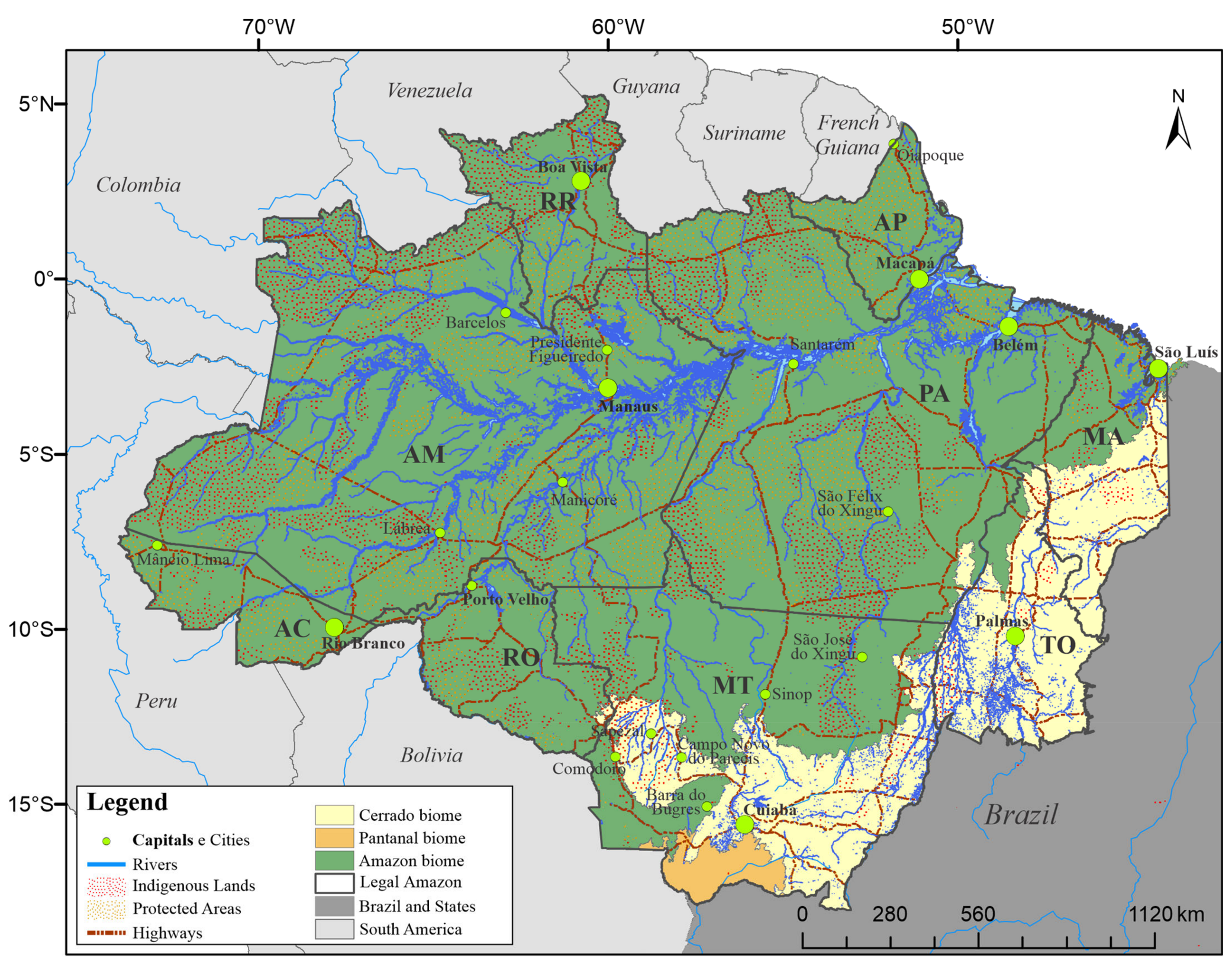
2.1. Study Area

The Brazilian Legal Amazon [3] comprises the States of Acre, Amapá, Amazonas, Mato Grosso, Rondônia, Roraima, Tocantins, Pará, and part of the State of Maranhão, located west of the 44^th meridian (Figure 1). It has an area of 5.02 M km², corresponding to 58.9% of the Brazilian territory [4]. The BLA contains three of the most important biomes in Brazil, the Amazon, Cerrado and Pantanal [4,48,49]. While the Amazon is covered mainly by tropical rainforests, Cerrado is a biome covered by a range of savannah-type vegetation, and Pantanal is covered by a mosaic of grasslands, flooded grasslands, wooded savanna, and riparian forests.

The predominant climate in the BLA is type “A”, or tropical, in which the average monthly temperature is never below 18 °C [51]. Three major types of climate are highlighted: the “Af” type (hot and rainy throughout the year), located in the northwest of the Brazilian Legal Amazon, the “ Am” (humid or sub-humid tropical climate), from the northeast to the south, marking the transition between humid tropical climates and those with a long dry season in the southern flank, and the “Aw” type (tropical climate, with dry winter), between the south and east, predominantly in the States of Mato Grosso, Rondônia, Tocantins and Maranhão [52].

2.2. Data

2.2.1. Land Use and Land Cover Data

In order to quantify the temporal and spatial variations in land use and land cover in the BLA, we obtained the MCD12Q1 version 06 product from the Moderate Resolution Imaging Spectroradiometer (MODIS) sensor on board the Terra and Aqua satellites [53]. This product was chosen because of its high accuracy over time and its public availability [41,54,55,56,57]. The algorithm that processes the product (V006 Global 500 m Land Cover Type Product) is based on supervised decision tree classifications of MODIS Terra and Aqua reflectance data and provides global land cover types at yearly intervals in 500 m of spatial resolution [53]. It contains five types of land cover classification, which describe surface properties, in sequence, derived from the International Geosphere–Biosphere Programme (IGBP), University of Maryland (UMD), Leaf Area Index (LAI), BIOME-Biogeochemical Cycles (BGC), and Plant Functional Types (PFT) classification schemes. The Type 1 classification scheme, from IGBP, was used (

Table 1. Type 1 classification of MCD12Q1 product ¹.

Class	Color	Acronym	Description
1	05450a	ENF	Evergreen Needleleaf Forests: dominated by evergreen conifer trees (canopy >2 m). Tree cover >60%.
2	086a10	EBF	Evergreen Broadleaf Forests: dominated by evergreen broadleaf and palmate trees (canopy >2 m). Tree cover >60%.
3	54a708	DNF	Deciduous Needleleaf Forests: dominated by deciduous needleleaf (larch) trees (canopy >2 m). Tree cover >60%.
4	78d203	DBF	Deciduous Broadleaf Forests: dominated by deciduous broadleaf trees (canopy >2 m). Tree cover >60%.
5	009900	MF	Mixed Forests: dominated by neither deciduous nor evergreen (40–60% of each) tree type (canopy >2 m). Tree cover >60%.
6	c6b044	CS	Closed Shrublands: dominated by woody perennials (1–2 m height) >60% cover.
7	dcd159	OS	Open Shrublands: dominated by woody perennials (1–2 m height) 10–60% cover.
8	dade48	WSV	Woody Savannas: tree cover 30–60% (canopy >2 m).
9	fbff13	SV	Savannas: tree cover 10–30% (canopy >2 m).
10	b6ff05	GL	Grasslands: dominated by herbaceous annuals (<2 m).
11	27ff87	PW	Permanent Wetlands: permanently inundated lands with 30–60% water cover and >10% vegetated cover.
12	c24f44	CL	Croplands: at least 60% of area is cultivated cropland.
13	a5a5a5	UBL	Urban and Built-up Lands: at least 30% impervious surface area including building materials, asphalt and vehicles.
14	ff6d4c	NVM	Cropland/Natural Vegetation Mosaics: mosaics of small-scale cultivation 40–60% with natural tree, shrub, or herbaceous vegetation.
15	69fff8	PSI	Permanent Snow and Ice: at least 60% of area is covered by snow and ice for at least 10 months of the year.
16	f9ffa4	BN	Barren: at least 60% of area is non-vegetated barren (sand, rock, soil) areas with less than 10% vegetation.
17	1c0dff	WB	Water Bodies: at least 60% of area is covered by permanent water bodies.

¹ MCD12Q1 product [53].

) between 2009 and 2019, as it is the most complete classification considering the purposes of this study [41,53,56]. To avoid mixing up atmospheric carbon estimates from land cover and use classes, we did not use the ENF, DNF, OS, BN, CS and NVM classes, since they were smaller than 1000 km² for all years [54].

The parameters of time and space for each type of land use and land cover were calculated using JavaScript language as input in the Google Earth Engine platform [58]. For analysis of the carbon estimates, 10 points were randomly selected, representative of each class of land use and land cover in the BLA and for each year, so that it was ensured that a given point was always considered in the same class for all the years studied. This was needed in order to verify if the emissions induced by land use and land cover changes in the BLA surrounding these selected points were impacting the class. These points were collected by the Google Earth Engine platform, by using the “Inspector” tab. The points were approximated from 1 to 2 km per pixel [57].

2.2.2. Gross Primary Production (GPP)

To analyze the GPP across the land cover and use classes, we obtained the MYD17A2H product, which is a cumulative composite of the GPP values based on the efficiency of use of solar radiation by vegetation [14,59]. The MODIS algorithm converts (via a conversion efficiency look-up table) the absorbed photosynthetically active radiation (related to the total amount of leaf area) to carbon uptake [8,60]. The MYD17A2H MODIS 8-day cumulative GPP product (2009–2019; 11 years total) was acquired using JavaScript language as input in the Google Earth Engine platform [58]. The GPP values were converted from the cumulative value every 8 days to annual median values (g C m⁻² year⁻¹).

2.2.3. Carbon Dioxide Flux (CO₂Flux)

To estimate annual forests’ carbon dioxide fluxes (µmol m⁻² s⁻¹), we employed the carbon dioxide fluxes (CO₂Flux). This is a remote sensing-based empirical model based on the Normalized Difference Vegetation Index (NDVI) (Equation (1)) and the scaled Photochemical Reflectance Index (sPRI) (Equation (2)) vegetation indices. Negative values represent a CO₂ sink, while positive values represent a CO₂ source [18,34,42,61]. While NDVI reveals the vigor of photosynthetically active vegetation, in which it may be able to absorb carbon [34,42], the sPRI estimates the carotenoid pigments of the leaves, indicating their rate of carbon dioxide storage [41]. For the calculation of NDVI, spectral bands 1 (620–670 nm) for red and 2 (841–876 nm) for NIR were used, based on the product MOD09A1 (Equation (1)). The bands used from the MOD09A1 product have a spatial and temporal resolution of 500 m, 1 to 2 days, respectively [62]. To estimate the sPRI, spectral bands 3 (459–479 nm), for blue (B), and 4 (545–565 nm), for green (G), of the MOD09A1 product were used:

$$\mathrm{NDVI}= \frac{NIR-R}{NIR+R},$$

(1)

$$sPRI=\left[\left(\frac{B-G}{B+G}\right)+1\right]/2,$$

(2)

The CO₂Flux values (µmol m⁻² s⁻¹) were estimated annually by taking the annual median of the time series (Equation (3)). The factors used in the equation were calibrated based on the Eddy Covariance method in micrometeorological towers [34,42,61].

$${\mathrm{CO}}_2\mathrm{Flux}=13.63-66.207 \left(NDVI\times sPRI\right),$$

(3)

The annual median values were calculated between 2009 and 2019 using JavaScript language as input in the Google Earth Engine platform [58].

2.2.4. Atmospheric CO₂ Concentration (XCO₂)

The atmospheric CO₂ concentration (XCO₂) data were acquired from the Greenhouse Gases Observing Satellite (GOSAT) in order to evaluate the spatial and temporal behavior of XCO₂ over the 11 years (April 2009 to December 2019) in the BLA. The GOSAT calculates the average XCO₂ in the path of sunlight reflected by the surface [63,64]. The XCO₂ did not account for all land use and land cover classes, because it has a spatial resolution of 2.5°, or 278 km, at the equator, making it impossible to be detected by most classes [64].

2.2.5. Precipitation Data

To identify the patterns of precipitation from 2009 to 2019 in the different land use and land cover classes of the BLA, we used the English Climate Hazards Group InfraRed Precipitation with Station data (CHIRPS) data at 0.05° (±5.3 km) spatial resolution and daily temporal resolution [43]. This presents satisfactory data for the spatiotemporal evaluation of regional precipitation in the Amazon, mainly because this region lacks data from in situ meteorological stations [15,43]. The annual sum values were calculated between 2009 and 2019.

2.3. Analysis

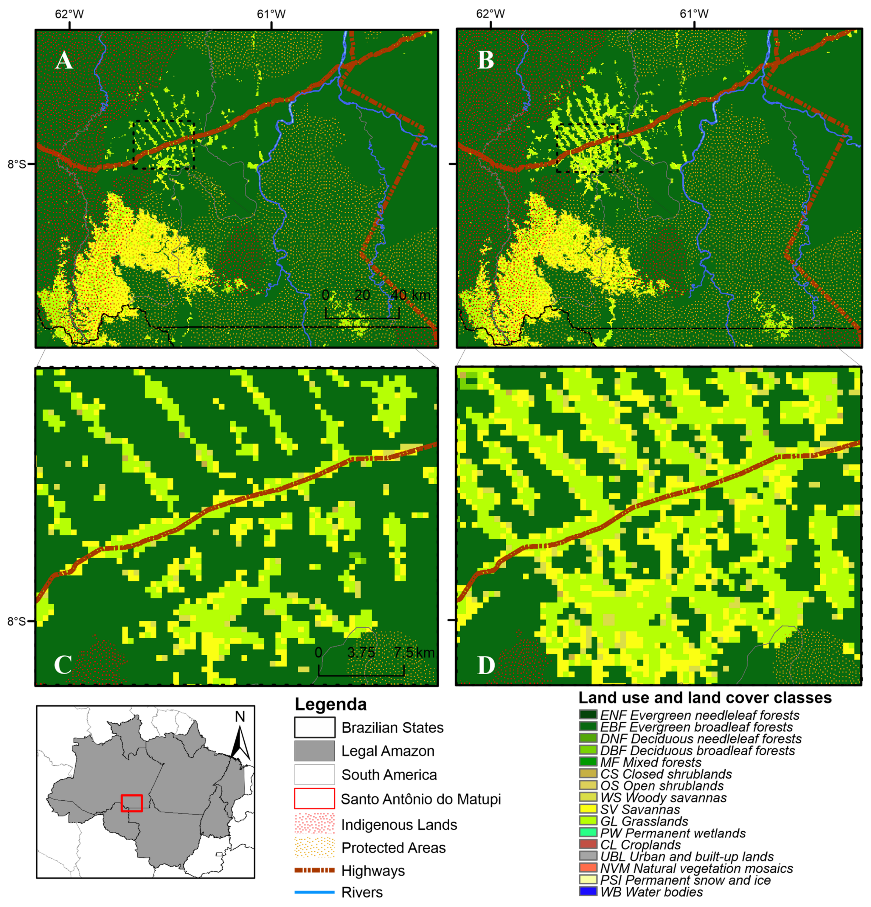
2.3.1. Land Use and Cover Change from 2009 to 2019

As a first step in understanding the carbon fluxes in the region, we analyzed the changes in the land cover and use classes across time from 2009 to 2019. We calculated the area occupied by each class in each year and determined the classes with highest area change.

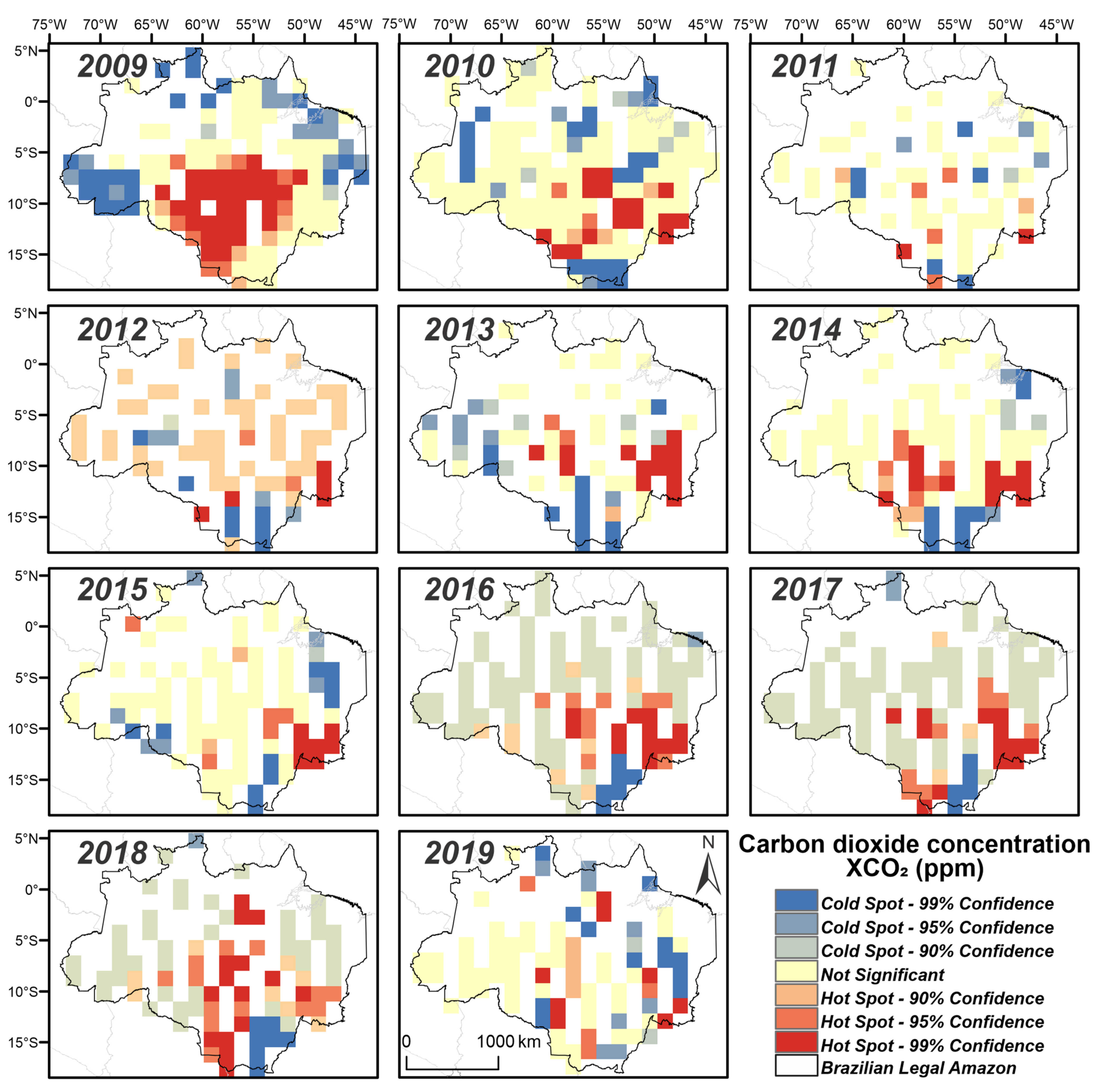
2.3.2. Spatial Clustering of Atmospheric Carbon

The spatial and temporal evaluation of XCO₂, hotspots were analyzed using the Getis-Ord method [65]:

$$G_i= \frac{{{\displaystyle \sum }}_{j=1}^n{w}_{i,j}{x}_j-\overline{X }{{\displaystyle \sum }}_{j=1}^n{w}_{i,j}}{S\sqrt{\left[\frac{n{{\displaystyle \sum }}_{j=1}^n{w}_{i,j}^2-{\left({{\displaystyle \sum }}_{i=0}^n{w}_{i,j}\right)}^2}{n-1}\right]}},$$

(4)

where G_i is the spatial dependence of incident i on all events n; x_j is the magnitude of variable X at incident location j in observations (n) (j can be equal to i); and w_ij is the weight value between event i and j representing the spatial interrelationship.

The Gi statistic identifies significant spatial groupings of high (hotspots) or low (coldspots) values in the observations, and was developed for data sets in which there is no global spatial autocorrelation [65]. Hotspot analysis was performed in ArcGIS version 10.8 [66], and points were transformed to raster to provide a better visualization.

2.3.3. Shapiro-Wilk Normality Test

The Co₂Flux, XCO₂ and GPP datasets comprising 11 years (2009 to 2019) from 10 land cover and use classes (EBF, DBF, MF, WSV, SV, GL, PW, CL, UBL and WB) were subjected to the Shapiro-Wilk normality test, with the “RVAideMemoire” package in R [67], which allows analysis of the normality of values within a group, thus verifying whether the data is parametrically distributed with greater assertiveness [68].

A Shapiro-Wilk normality test without considering groups was also performed; however, not considering groups for larger samples of data can introduce errors and the RVAideMemoire::byf.shapiro() function can help to verify this. This function is an excellent choice for examining questions about normality by breaking factor-type object variables [69].

To allow a comparative view between the three variables (GPP, CO₂Flux and Rainfall) and complement the normality test, a histogram was generated. This presents distribution and frequency in relation to the center [69].

2.3.4. Variability of Carbon Fluxes in between Land Cover and Use Classes

To compare how carbon fluxes varied between the different land cover and use classes, we employed the non-parametric one-way Anova Kruskal-Wallis test. This test ranks the values, and groups with different distributions can be compared based on their medians [70,71]. The Kruskal-Wallis test was used to identify which parameters (land use and land cover classes or years) showed significant differences between the variables (GPP, CO₂Flux and Rainfall) across the BLA [70,72]. The magnitude of changes was calculated by the percentage difference between the medians [70,71].

To identify in which groups these observed differences occurred, a Dunn post-hoc test was performed [70,72], with adjustment of the p-value by the Bonferroni method, an adjustment for multiple comparisons. The Bonferroni method is more conservative and guarantees the difference between these groups. For comparisons between groups with non-parametric data, the “rstatix” package in R was used [67]. Boxplots and scatterplots showing the variability of GPP, CO₂Flux and Rainfall amongst the 10-land use and land cover classes (EBF, DBF, MF, WSV, SV, GL, PW, CL, UBL and WB) were also produced These analyzes were performed in R software using the GGEBiplotGUI package [67].

2.3.5. Cluster Analysis

To evaluate the affinities between land use and land cover and carbon emission/absorption and precipitation variables, we employed a cluster analysis based on the principal components and dendogram methods [73]. The cluster analysis is based on unsupervised learning, in which the data are segmented into groups based on an exploratory analysis, in case of absence of a dependent variable, or doubts about it. In this way, cluster performs segmentation in the dataset through its attributes, organizing and facilitating visualization by grouping variables with similarities. It also helps in the detection of anomalies or outliers. Groups of clusters that minimize dissimilarity or minimize total sums of squares within groups are also known as Sum of Squared Deviation (SQD) [74]. At each step of the procedure, the groups were formed in such a way that the resulting solution has the smallest SQD within the groups. The union of all possible group pairs was considered. The two groups that resulted in a smaller increase in SQD were grouped to form a single group that brings together all subjects [75,76].

Clusters were generated using scaled GPP, CO₂Flux and Rainfall data for each use and land cover class between 2009 and 2019. For this, the Euclidean distance and Ward’s hierarchical method were used [74,75,76]:

$$d_e={\left[{\displaystyle \sum }_{j=1}^n{\left(P_{p.j}-P_{k.j}\right)}^2\right]}^{\frac{1}{2}},$$

(5)

where d_e is the Euclidean distance, and P_p and P_k are the variables j of subjects p and k.

Principal component analysis was also performed to examine whether the variables GPP, CO₂Flux and Rainfall, derived from remotely sensed data, could help characterize different land use and land cover in the BLA [73,77].

2.3.6. Trend Analysis

To identify years showing a trend over the time series (2009–2019) for each variable, we employed the Mann Kendall (MK) test [78,79] and the Pettitt test [80]. MK identifies whether time series values tend to increase or decrease over time, or whether the central value in the distribution of time series data changes over time. The Pettit test shows when this tend occurred or confirms the stationarity of the historical series. This non-parametric test uses a version of the Mann-Whitney test, from which it is verified whether two samples X₁,…,X_t and X_t+1,…,X_t fit to the same population [80]. The U_t,T statistic counted the number of times that a member of the first sample is greater than the member of the second, according to Equation (6). U_t,T is calculated for the values of 1 < t < T, and k(t) is given by Equation (7).

$$U_{t,T}=U_{t-1,T}+{\displaystyle \sum }_{j=1}^{T}sgn\left(X_i-X_j\right),$$

(6)

$$k\left(t\right)=MA{X}_{1\le t\le T}\left|U_{t,T}\right|,$$

(7)

where sgn(x) = 1 for x > 0; sgn(x) = 0 for x = 0; and sgn(x) = −1 for x < 0.

The Pettitt test locates the point at which an abrupt change occurred in the historical series, the t where the maximum of k(t) occurs, resulting in Kcrit, or critical values (Equation (8)), in the mean of a temporal series. Its significance was calculated by Equation (9).

$$K_{crit}=\pm \sqrt{\frac{-ln\left(\frac{p}{2}\right)\left(T^3+T^2\right)}{6}},$$

(8)

$$p-value\cong 2exp\left\{\frac{-6k{\left(t\right)}^2}{\left(T^3+T^2\right)}\right\},$$

(9)

For the application of the Mann-Kendall and Pettitt tests, the “trend” and “ManKendall” packages were used in the R version 4.1.2 [67].

3. Results

3.1. Land Use and Land Cover Changes

The nomenclatures of the land use and land cover classes can be found at the bottom of Table 1 and

Table 2. Area, in km², of the land use and land cover classes of the BLA between 2009 to 2019.

Classes	ENF 1	EBF	DNF	DBF	MF	CS	OS	WSV
2009	126.49	3,374,351.77	0.74	9370.81	2685.39	313.90	170.61	219,487.50
2010	110.76	3,363,598.69	0.00	10,976.39	2837.62	320.71	100.80	223,691.17
2011	114.47	3,356,746.45	0.00	11,235.69	2671.78	332.30	64.89	226,820.70
2012	119.11	3,351,448.68	0.00	12,161.83	2525.68	383.75	59.83	225,836.89
2013	132.59	3,346,877.56	0.00	12,592.50	2292.61	419.95	60.18	225,740.05
2014	141.44	3,341,805.65	0.00	13,785.02	2265.73	470.68	65.79	222,678.17
2015	144.93	3,332,142.23	0.00	15,043.02	2275.90	525.03	86.63	218,875.11
2016	143.43	3,320,505.98	0.00	15,357.38	2206.02	728.91	102.35	218,150.23
2017	157.83	3,318,989.15	0.24	16,228.36	2122.46	830.99	98.89	212,146.05
2018	148.00	3,311,486.93	0.00	15,606.63	1571.92	883.70	72.94	217,815.19
2019	122.77	3,307,899.08	0.00	16,282.29	1554.08	823.63	59.67	219,497.52
Minimum	110.76	3,307,899.08	0.24	9370.81	1554.08	313.90	59.67	212,146.05
Maximum	157.83	3,374,351.77	0.74	16,282.29	2837.62	883.70	170.61	226,820.70
Mean	132.89	3,338,713.83	0.09	13,512.72	2273.56	548.50	85.69	220,976.23
Classes	SV	GL	PW	CL	UBL	NVM	BN	WB
2009	814,410.32	427,688.15	42,969.10	46,468.92	3214.24	760.86	118.81	76,486.03
2010	814,458.43	430,814.48	43,318.25	47,845.75	3218.21	752.73	119.44	76,460.22
2011	820,451.11	424,921.60	44,032.14	50,617.98	3222.43	775.05	114.60	76,502.45
2012	828,404.93	419,508.25	44,750.54	52,640.53	3225.15	807.99	120.01	76,630.49
2013	831,246.14	418,879.58	45,302.60	54,131.14	3227.63	837.67	121.21	76,762.25
2014	829,377.20	425,725.68	45,899.51	55,250.24	3232.08	884.83	126.88	76,914.74
2015	825,109.87	440,198.42	46,546.19	56,517.91	3234.31	892.63	139.62	76,891.86
2016	821,453.22	454,674.01	47,346.18	56,951.16	3236.53	915.08	166.13	76,687.03
2017	814,680.05	466,125.38	46,820.45	59,371.91	3241.23	867.62	177.82	76,765.22
2018	792,856.33	489,266.49	47,711.84	60,107.64	3245.43	798.85	160.64	76,891.15
2019	777,734.68	504,234.83	47,931.70	61,454.07	3249.64	668.03	142.10	76,969.55
Minimum	777,734.68	418,879.58	42,969.10	46,468.92	3214.24	668.03	114.60	76,460.22
Maximum	831,246.14	504,234.83	47,931.70	61,454.07	3249.64	915.08	177.82	76,969.55
Mean	815,471.12	445,639.72	45,693.50	54,668.84	3231.53	814.67	137.02	76,723.73

¹ Evergreen Needleleaf Forests (ENF); Evergreen Broadleaf Forests (EBF); Deciduous Needleleaf Forests (DNF); Deciduous Broadleaf Forests (DBF); Mixed Forests (MF); Closed Shrublands (CS); Open Shrublands (OS); Woody Savannas (WSV); Savannas (SV); Grasslands (GL); Permanent Wetlands (PW); Croplands (CL); Urban and Built-up Lands (UBL); Natural Vegetation Mosaics (NVM); Barren (BN); and Water Bodies (WB).

. The greatest extensions in area were observed for the classes EBF, SV, GL, WSV, WB, CL, PW, DBF, UBL and MF, from 3.37 M to 1.55 K km², respectively, while ENF, DNF, OS and BN classes were smaller than 200 km², and CS and NVM, were smaller than 1000 km². The PSI class was not observed (Table 2, Figure S1).

From 2009 to 2019, there were increases in the areas of DBF (6911.48 km²), CS (509.74 km²), WSV (10.02 km²), GL (76,546.68 km²), PW (4962.60 km²), CL (14,985.15 km²), UBL (35.40 km²), BN (23.29 km²) and WB (483.52 km²) and, on the other hand, decreases in the areas of ENF (3.72 km²), EBF (66,452.69 km²), MF (1131.31 km²), OS (110.94 km²), SV (36,675.64 km²) and NVM (92.83 km²).

The EBF had the largest area (3.34 M km²), observed in the center, east and north of the BLA. It is also that which suffered the majority of the losses over the study period, of 66,452.69 km². Considering the total study area, the EBF represented 67.28% in 2009 and dropped to 65.95% in 2019. This evidences a reduction of ~2%, as an annual mean of 6645.27 km² in land use and land changes (Figure 1, Table 2).

Larger areas of SV, GL and WSV were observed in the northeast to south of BLA, representing the second, third and fourth largest extensions, close to each other. These classes were observed from the northeast, near São Luís—MA, to the south of the BLA, as well as in the region of Boa Vista—RO (Figure 1). The DBF and MF classes were observed closer to the SV, GL and WSV classes. In greater concentration, the DBF was observed in the south of Mato Grosso state (MT) and in the central part of Maranhão, and MF in the southeast of Mato Grosso and Pará. The CL was the sixth largest in area and was observed mainly in the southern flank of the BLA (Figure 1 and Figure 2).

The SV was observed close to the WB, the fifth largest class, and federal highways throughout the studied area, while a strong highlight for the GL class was observed in the middle east and in the state of Roraima. The greatest representation of this class was in the Cerrado and Pantanal biomes, especially in the transitions to the Amazon biome (Figure 1 and Figure 2).

Decrease for the SV and WSV areas was also observed, of 53,511.46 km² from 2013 to 2019 and 14,674.65 km² from 2011 to 2017, respectively, while an increase was observed for the GL class after 2013 and until 2019, of 85,355.24 km² (Table 2).

The CS and OS classes were observed as adjacent to the other classes, with some scattered points to the north, east and south regions of the BLA. The NVM class was strongly related to the CL class, so that both were observed in greater numbers from the northeast to the south (Figure S1). The BN class was observed in the east of the BLA, close to the Tocantins and Araguaia rivers (WB class), in regions where the sand was exposed, forming small beaches [4,50] (Figure 1 and Figure 2). The PW class appeared to be related to the WB class, one adjacent to the other, and it was observed throughout the studied area in branched continuous formats, represented by the largest rivers in the region, such as the Amazon, Negro, Solimões, Araguaia and Tocantins (WB class) [4,81]. The UBL class was also observed throughout the studied area in small, scattered spots. The DNF class was observed in the northwest region of the BLA (Figure S1), north of the city of Barcelos—AM, at the southern intersection between the Serra do Araçá State Park and Amazonas National Forest PA [4,50]. These points were observed only in 2009 and 2017, and represented a decrease of 0.50 km² in the area (Figure 1 and Figure 2).

Figure 2 highlights the district of Santo Antônio do Matupi (state of Amazonas) comparing years 2009 (Figure 2A,C) and 2019 (Figure 2B,D). This is typical example of a larger land use and land cover change from forest to anthropized areas. The district of Santo Antônio do Matupi is located in the south of the State of Amazonas, bordering the States of Mato Grosso and Rondônia, close to the “Transamazônica 230” highway. As mentioned above, this site was especially chosen because it presented significant forest losses, mainly from EBF, and the increase in anthropized areas, the GL classes more intense around the “Transamazônica 230” highway. The district of Santo Antônio do Matupi is located north of the Campos Amazônicos National Park and the Aripuanã National Forest PA and south of the Campos de Manicoré Environmental PA and the Manicoré Biological Reserve [82].

Such land use change is close to the Ils Diahui, Pirahã, Sepoti, Tenterim Marmelos, and Tenterim do Igarapé Preto, which are also in zones of environmental, ecological, and social preservation [2]. However, Santo Antônio do Matupi is an important timber exploitation region. This fact was confirmed by Duarte et al. [83], who observed losses of primary forests in Santo Antônio do Matupi, with the most critical period of deforestation rates recorded between 2004 and 2018, when 63.28% of the deforested area was converted into pastures. In 2010, it was one of the ten highest contributing communities to the economy of Amazonas, in 2014 the fourth largest cattle producer in the State, and the largest producer of wood, with a herd increase of 800% and a deforested area of more than 676.5 km² [83,84].

3.2. Spatial Variability of Carbon

Higher GPP values were found in the western, central, and northern regions of the BLA, with averages between 40 and 44 gC m⁻², as can be seen mostly for the EBF class (Figure S1 and Figure 4 and Table 2). The maximum values of GPP, represented by navy-blue color, were found in the northeast of the BLA, in the regions of the State of Amapá and northwest of Pará, near to the equator [4,50], with annual maximums between 80.55 gC m⁻² (2009) and 88.2 gC m⁻² (2015) (Figure S2).

Values close to zero were observed on the border from east to south of the studied area and in the State of Roraima. In the year 2016, a greater intensity of values and greater extension in relation to other years were observed, represented by the orange color in the Southeast and mostly related to the land use classes SV, GL and WSV. In addition, the MF, SV and WSV decreased in extension while GL, CL, UBL, PW and WB increased, with these land use and land cover changes related to a decrease in the GPP values in the studied period (Figure S2, Table 2).

Lowest CO₂Flux values were found in the central and western regions of the BLA. Such values, often negative, were represented by the forest classes EBF, DBF, MF and WSV, with EBF class being the main one, due to its extension. In the center of the study area, higher carbon absorptions were observed, mainly in 2019, of −8.35 µmol m⁻² s⁻¹ to the EBF class similar to observed by Rossi et al. [34] in 2017. The highest values of CO₂Flux were observed in the transition from northeast to south, where the SV, GL, CL, and PW classes are located (Figure S3).

The spatial distribution of XCO₂ hotspots was concentrated in the central and southeastern region of the BLA (Figure 3). As observed for GPP (Figure S2), in 2009 and 2016, the Southeast region displayed a large concentration of 99% confidence hotspots, frequent in most of the studied years. In the central-north regions of State of Mato Grosso, hotspots were observed in 2015 and 2016 and had higher XCO₂ spatial atmospheric patterns than 2017 and 2018 (Figure 3).

On the other hand, coldspots were mostly distributed from the north and west of the BLA, and in part to the south, compared with negative CO₂flux and positive GPP. These represent the significant negative values that resulted in a more intense grouping of low values, in a typically forested area as EBF class. Coldspots were also observed from 2010 to 2018 in the southern region, with emphasis on the years 2016 to 2018, in which there was a large percentage of coldspots at a 90% confidence level, which contrasted with preceding years (Figure 3).

For all the years studied, the central, western, and northern parts of the BLA had higher rainfall, except for the extreme northern area, in Roraima. Annual maximums were observed in the Northwest for all years and in the Northeast for the years 2009 to 2013 and 2017 to 2019. The minimum precipitation was observed on the east to south flanks for 2015 to 2017. The lowest precipitation was in 2015 due to a severe drought event in Amazonia [13,40]. The maximum values of precipitation were found in the north, close to the Equator, except for 2014 to 2016 and 2019, for the State of Amapá (Figure S4).

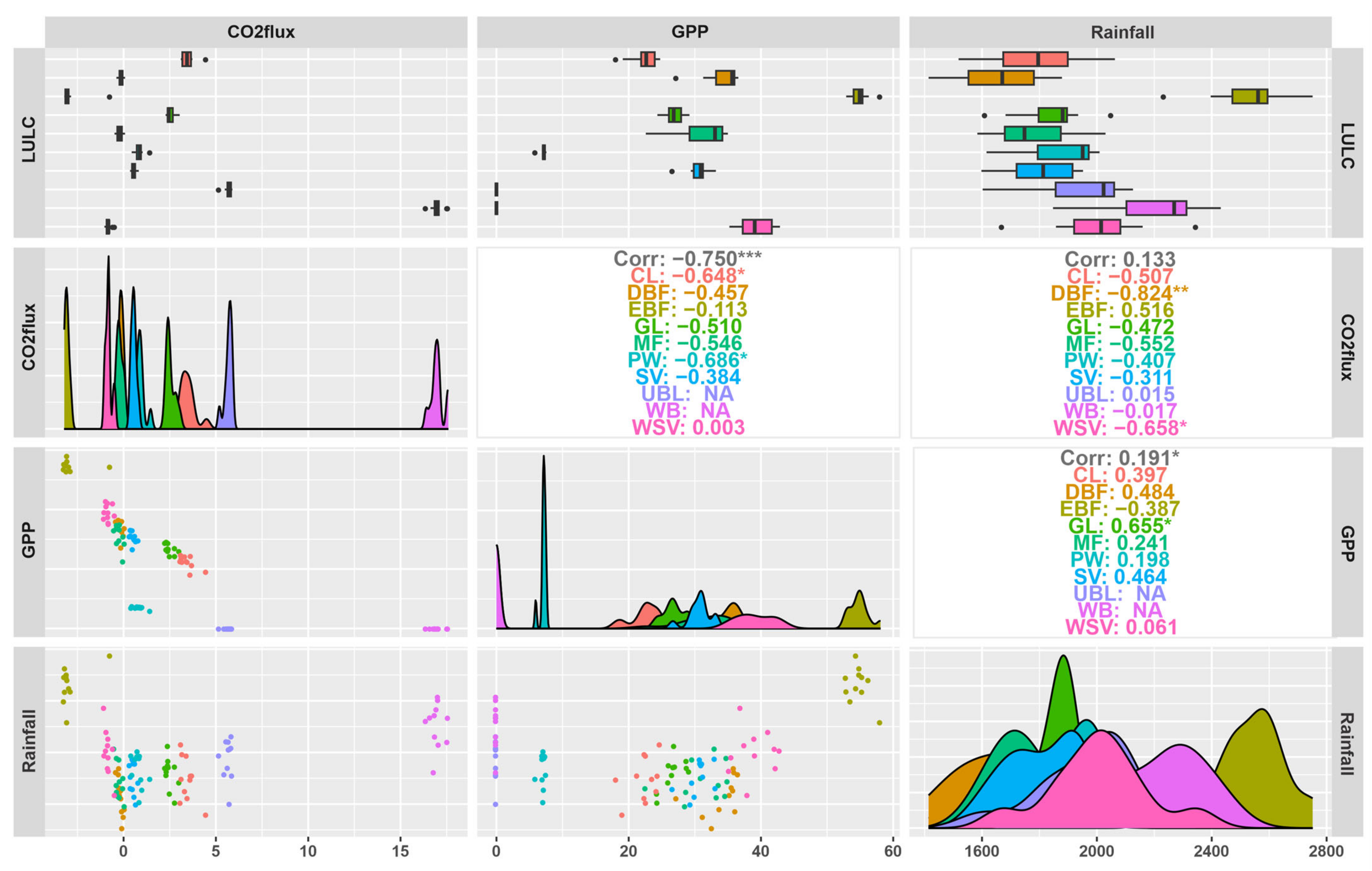
3.3. Statistical Analysis

According to

Table 3. p-value of the multivariate Shapiro-Wilk normality test non-grouping and grouped by classes and years for the variables GPP, CO₂Flux and Rainfall.

Varible	Grouped by Classes
	Non- Grouping	EBF	DBF	MF	WSV	SV	GL	PW	CL	UBL	WB
GPP	0.000 ***	-	-	-	-	-	-	-	-	-	-
CO2Flux	0.000 ***	0.000 ***	0.936	0.658	0.204	0.874	0.047 **	0.474	0.007 ***	0.692	0.464
Rainfall	0.000 ***	0.793	0.786	0.436	0.952	0.229	0.577	0.0794 *	0.695	0.117	0.424
	Grouped by Year
	2009	2010	2011	2012	2013	2014	2015	2016	2017	2018	2019
GPP	0.483	0.406	0.439	0.390	0.506	0.567	0.470	0.493	0.478	0.421	0.398
CO2Flux	0.004 ***	0.007 ***	0.005 ***	0.006***	0.000 ***	0.009 ***	0.005 ***	0.008 ***	0.008 ***	0.005 ***	0.006 ***
Rainfall	0.192	0.824	0.715	0.2067	0.007 ***	0.015 **	0.002 ***	0.006 ***	0.058 *	0.062 *	0.144

*, ** and ***: significant at 10, 5 and 1% probability by Shapiro-Wilk normality test. Evergreen Broadleaf Forests (EBF); Deciduous Broadleaf Forests (DBF); Mixed Forests (MF); Woody Savannas (WSV); Savannas (SV); Grasslands (GL); Permanent Wetlands (PW); Croplands (CL); Urban and Built-up Lands (UBL) and Water Bodies (WB).

, the non-grouping demonstrated non-normal distribution for the variables, as they presented a p-value > 5% from the Shapiro-Wilk test [68]. However, the data were normal when grouped by year for GPP and Rainfall, and when grouped in classes for CO₂Flux and Rainfall (precipitation). It was not possible to verify the normality of the grouping in classes for GPP, because WB and UBL data showed null values, as they do not represent vegetative classes [41].

The EBF, GL and CL represented the greatest variabilities for CO₂Flux, and PW for Rainfall within the years 2013 to 2018. The Shapiro-Wilk grouped normality test indicates that statistics could be applied to normal data distribution to GPP or Rainfall over the years. The same occurred in the case of the Rainfall variable in different land use classes (Table 3).

Complementary to the Shapiro-Wilk normality test, the histogram showed the data distribution and in which position was its highest frequency. This was observed between 20 and 40 gC m⁻², for the GPP, from –1 to 2.5 µmol µmol m⁻² s⁻¹, for CO₂Flux, and from 1600 to 2200 mm, for Rainfall variables. Based on the histogram, it was also possible to identify unexpected values and trends (Figure S5).

Since the multivariate Shapiro-Wilk normality test and the histogram (Table 3 and Figure S5) presented non-parametric data [69,71], we decided to apply the Kruskal-Wallis and Dunn tests to compare groups of classes. The boxplots grouped by classes and by years were performed (Figure 4). The median values of the classes and years groups are shown in Table S1.

Differences between land use classes were observed for GPP (X² = 103.96), CO₂Flux (X² = 106.73) and Rainfall (X² = 65.12) by the Kruskal-Wallis test (p < 0.05). The Dunn’s post-hoc test showed that differences in GPP were between EBF and CL, GL, UBL, PW and WB. The DBF and WSV classes were different from UBL, PW and WB. MF and SV were different from UBL and WB. It is also interesting to observe that EBF did not differ from the DBF, MF, SV and WSV classes, all these considered as forest classes, which had medians of 52.90, 34.68, 31.53, 31.32 and 39.84 gC m⁻², respectively. Outliers below the minimum values were observed for SV, DBF, CL and PW, of 23.53, 22.90, 16.88 and 0.43 gC m⁻², in 2016, respectively (Figure 4a and Table S1).

The EBF showed the highest value of 52.90 gC m⁻² and an outlier above the maximum values was observed, of 55.43 gC m⁻², in 2018. The PW had the lowest GPP values, of 0.6 gC m⁻². The amounts of total carbon absorbed in an area is related to the area extension and these were, on average, 176.63, 25.54, 11.46, 8.80, 1.17, 0.47, and 0.07 Tg C year⁻¹ for EBF, SV, GL, WSV, CL, DBF, and MF classes, respectively. The UBL and WB classes did not absorbed any carbon as these do not represent vegetation areas, and the PW class absorbed only 0.03 Tg C year⁻¹ (Figure 4a and Table S1).

For the CO₂Flux variable, the Dunn test and the boxplot showed a difference between EBF and CL, GL, UBL, PW and WB, and a similarity between forest classes DBF, MF and WSV, except for SV, with values of −3.09, −0.06, −0.26, −0.65 and 0.28 µmol m⁻² s⁻¹, respectively. DBF and MF classes were different from CL, UBL and WB. The WSV class was different from CL, GL, SV, UBL, PW and WB, while SV was also different from WB. PW was different from WB but similar to UBL. The DBF, MF and SV classes oscillated between negative and positive values, while PW was positive, but also close to zero. Certainly, these values made DBF and MF more similar, as also occurred for SV and PW, as CO₂Flux values increased from forest classes to more anthropic-use classes, following the order EBF, WSV, MF, DBF, SV, PW, GL, CL and UBL (Figure 4b and Table S1).

In the Rainfall, the Dunn test specified that there was a difference between EBF and DBF, CL, GL, MF, SV, and PW, but not for UBL and WB, which had values above 1605 mm. In addition, the DBF, MF and SV classes was different from WB, and DBF was also different from WSV, because DBF, MF, SV, GL, and CL were the classes with the lowest precipitation, with values below 1533 mm. WSV, PW and UBL had averages between 1902 and 1929 mm, while EBF and WB were 2473 and 2234 mm (Figure 4b and Table S1).

The Cluster analysis was carried out to improve the visualization of the groupings, which demonstrated that EBF was the most distant grouping amongst the land use and land cover types of the BLA, and that it was closest to DBF and WSV for those variables capable of measuring absorption and above ground carbon stock, finally being grouped according to the rainfall regime of these classes (Figure S6).

The GL and CL classes were similar because, despite representing median GPP values of 25.71 and 21.44 gC m⁻², CO₂Flux values were always positive at 2.83 and 3.50 µmol m⁻² s⁻¹, respectively. The UBL and WB groups represented the highest emissions through CO₂Flux, of 5.76 and 15.92 µmol m⁻² s⁻¹, respectively, and no biomass production (GPP = 0), and PW merged with this group, mainly due to not producing biomass efficiently, with only 0.6 gC m⁻² over the years (Figure 4a,b and Figure S3).

The MF and SV classes were similar because they produced more biomass than the GL and CL groups, 31.53 and 31.32 gC m⁻², but oscillated between carbon absorption and emission, by CO₂Flux, between 0.11 and −0.53, and 0.69 and −0.08 µmol m⁻² s⁻¹, respectively, as well as what is observed for DBF, with GPP only a little higher, at 34.68 gC m⁻². WSV showed higher biomass production compared to previous classes, of 39.84 gC m⁻², but absorbed carbon every year (CO₂Flux < 0), as well as EBF; however, this latter class was that which obtained the highest carbon absorption by GPP and CO₂Flux, combined with the highest amount of Rainfall compared to the other classes (Figure 4a–c and Figure S3).

In the Kruskal-Wallis and Dunn tests for comparison between years in the BLA, only the Rainfall variable showed a significant difference (X² = 28.61, p < 0.05). The Dunn test showed that this difference was between 2013 and 2015 and between 2015 and 2018, which had values of 2092, 1689 and 2026 mm, respectively. The Rainfall values decrease for the different classes following this order: EBF, WB, WSV, UBL, PW, GL, SV, CL, MF and DBF, with maximums of 2792 (2013), 2453 (2013), 2182 (2011), 2120 (2018), 2098 (2011), 2091 (2009), 1983 (2013), 2074 (2018), 2016 (2013) and 1941 (2013), and lows of 2163 (2015), 1895 (2015), 1706 (2015), 1605 (2015), 1702 (2010), 1533 (2015), 1530 (2015), 1527 (2010), 1528 (2010) and 1475 (2010) mm. Outliers between 2013 and 2015, above the maximum values and lower that the minimum values, were observed for the Rainfall variable, with EBF being the class responsible for the above outliers (Figure 4f and Figure S3).

The GPP values were in descending order from the forest classes to the most anthropic classes as follows, EBF, WSV, DBF, MF, SV, GL, CL and PW, with maximums of 55.43 (2018), 43.10 (2018), 39.20 (2018), 36.23 (2017), 36.00 (2019), 31.25 (2019), 24.03 (2018) and 0.73 (2014), and minimums of 50.23 (2013), 35.53 (2016), 22.90 (2016), 22.35 (2016), 23.53 (2016), 16.25 (2016), 16.88 (2016) and 0.43 (2016) gC m⁻². The EBF, DBF, WSV and CL classes had the highest GPP in 2018, but in general the maximum values were observed after 2017, while the minimum values were in 2016. In the EBF class, a decrease in GPP was observed shortly after drought events, from 53.59 gC m⁻², in 2010, to 52.89 and 52.99 gC m⁻², in 2011 and 2012, and from 58.07 gC m⁻², in 2015, to 55.35 gC m⁻², in 2016 (Figure 4d and Figure S3).

The EBF and WSV classes had lower CO₂Flux in 2014, of −3.55 and −0.98 µmol m⁻² s⁻¹, while DBF and MF were −0.28 (2018) and −0.53 (2009) µmol m m⁻² s⁻¹, respectively. Outliers above the maximum values were seen for all years in the CO₂Flux variable for the WB class. The DBF and MF classes had minimums in 2013 and maximums in 2012 and 2010, respectively (Figure 4e and Figure S3).

The years 2014 and 2018/19 showed the highest GPP averages of 24.26, 26.24 and 26.03 gC m⁻², respectively, and the lowest CO₂Flux. In addition, the years with the lowest Rainfall values, such as 2010 and 2015/16, demonstrated the dependence of these indices on climatic factors, with lower GPP averages, of 22.76 (2015) and 19.24 (2016) gC m⁻², and higher CO₂Flux of 2.80 (2010) µmol m⁻² s⁻¹ (Figure 4d–f and Figure S3).

The correlation between the CO₂Flux and GPP variables was strong and negative, at −0.75, which also means that the increase in one influences the decrease in the other, and was statistically significant for the CL and PW classes, at −0.65 and −0.69, respectively. Low correlation between the variables CO₂Flux and GPP with Rainfall was observed and this was due to the non-linearity between them, seen the scatterplot at the lower left part of the graph (Figure 5).

In the correlation between CO₂Flux and Rainfall, the DBF and WSV classes had a strong negative correlation of −0.82 and −0.66, which demonstrates that the increase in Rainfall values causes a decrease in CO₂Flux values. Only EBF and UBL showed a positive, though weak, correlation, which showed that the increase in Rainfall values can increase de CO₂Flux values. In the correlation GPP with Rainfall variables, only EBF presented a negative correlation, also weak; a strong and positive correlation was observed for the GL class of 0.66 (Figure 5).

The first two principal components (Dim1 and Dim2), which analyzed the cluster in the classes and variables, accounted for 58.4% and 35.4% of the total variance between data. Greater affinity was observed for GPP with EBF and with WSB and was more distant for WB and UBL. The CO₂Flux variable was more associated with the WB class, also being close to the UBL due to the higher values for this variable. The other classes with the presence of vegetation ranged between negative and positive or were close to zero, which may be related to the poor ability of the CO₂Flux index to characterize these classes. In addition, Rainfall was closer to the EBF and WB classes, as they were those that had values above 2200 mm for all years of the studied period (Figure 6).

With the purpose of evaluating the existence of monotonic trends in historical series of the three variables (GPP, CO₂Flux and Rainfall) over 10 classes of land use and land cover of the BLA (EBF, DBF, MF, WSV, SV, GL, PW, CL, UBL and WB), the Mann-Kendall test was used, which is more robust in terms of deviations from normality and in non-stationarity of historical series data, compared to other parametric tests [54,56]. Trend analysis was performed by observing the Z value. Identification of years with a trend over the time series (2009–2019) for each variable was performed using the Pettitt Test. Points were selected where the classes had not changed over the years but were influenced by changes in the uses of adjacent classes (

Table 4. p-value for the Mann-Kendall and Pettitt tests for GPP, CO₂Flux and Rainfall variables in the BLA, grouped by land use and land cover.

Classes	GPP			CO2Flux			Rainfall
	Mann-Kendall	Z	Pettitt	Mann-Kendall	Z	Pettitt	Mann-Kendall	Z	Pettitt
EBF	0.07 *	1.80	0.04 **	0.24	−1.18	0.56	0.56	0.58	0.79
DBF	0.58	0.55	0.42	0.64	−0.46	1.00	0.60	0.52	0.41
MF	0.44	0.77	0.01 ***	0.54	−0.61	0.80	0.76	0.30	0.13
WSV	0.29	1.06	0.28	0.92	0.10	1.00	0.21	−1.27	0.73
SV	0.94	0.07	1.00	0.28	−1.07	0.86	0.66	−0.43	1.00
GL	0.63	0.48	0.83	0.59	−0.54	1.00	0.19	−1.30	0.19
CL	0.22	1.22	0.10	0.39	−0.86	0.52	0.41	0.83	0.31
PW	0.74	−0.33	1.00	0.97	−0.04	1.00	0.34	−0.95	1.00
UBL	-	-	-	0.12	1.55	0.47	0.76	0.30	0.78
WB	-	-	-	0.76	−0.30	1.00	0.58	−0.56	0.65

*, ** and ***: significant at 10, 5 and 1% probability by Mann-Kendall and Pettitt tests.

).

For the EBF class, Mann-Kendall demonstrated an increase in GPP (p < 0.1) and Pettitt showed that 2013 (p < 0.05) had an increase in its values over the years. For other vegetative classes, such as MF (p < 0.01), this increase was observed mainly after 2016/17. Despite the observation of changes in land use and land cover, in general, no significant trends were detected in the data for the GPP, CO₂Flux and Rainfall variables by the Mann-Kendall and Pettitt tests. However, according to the Z value, a positive tendency for GPP was observed, mainly for EBF, WSV and CL, and a negative trend for CO₂Flux, for EBF and SV, throughout the years studied. A negative trend was also observed, that is, a decrease in Rainfall values over the years, for WSV, SV, GL, PW, and WB (Table 4).

4. Discussion

4.1. The Effect of Changes in Land Use and Land Cover on Indigenous Lands, Protected Areas and Other Important Areas of Conservation

In general, the land use and land cover classifications using the MCD12Q1 product showed good accuracy for the BLA over the years studied. Studies report its high accuracy in classifying land use and land cover, mainly for relatively stable classes such as water and forests [41,54,55,56,57].

The reduction observed in the forest classes, EBF, WSV and SV, was from 67.28%, 4.38%, 16.24%, in 2009 to 65.96%, 4.38%, 15.51%, in 2019, respectively, while anthropized areas, such as GL and CL, increased from 8.53% and 0.92%, in 2009, to 10.05% and 1.22%, in 2019, respectively, possibly characterizing deforestation [85].

The EBF was observed in the center, west and north of the Legal Amazon. As it is the largest type of forest in the BLA, the EBF class represents an important carbon sink [4,41,86]. This class is also known as Dense Ombrophylous Forest or Tropical Pluvial Forest [87], is the main phyto-physiognomy of the Amazon biome, and occurs in tropical, or even equatorial, areas where high rainfall is regularly distributed throughout the year [49,51,52,87]. This type of forest is mainly preserved over Indigenous Lands (IL) and Protected Areas (PA) in the region [2,25,26,27,29].

The indigenous lands in the Brazilian Amazon cover 27% of the area with forests, are home to 173 ethnic groups and are fundamental for the physical and sociocultural reproduction of indigenous peoples, in addition to being important areas for the conservation of regional and global biodiversity [2,25]. In addition, IL and PA correspond to half of the total forest area of the BLA, playing important roles in forest and biodiversity conservation and climate mitigation [2,26,27].

In Brazil, deforestation rates, and consequent changes in land use and land cover in forest areas protected by IL and PA are up to ten times lower than in areas without environmental protection. This is because these areas have greater forest cover and lower deforestation pressure compared to areas without environmental protection, which tend to have high deforestation pressures [2].

Similar to the EBF class, the SV and WSV represent the main phyto-physiognomies of the Cerrado biome [49,87] and both have suffered a reduction of 68,186.11 km². The SV class was observed in the Cerrado and Pantanal biomes and in their transitions to the Amazon biome [2,44,50], close to ILs, PAs and highways from the north, in the Parque do Tumucumaque IL, in the State of Pará, around the BR-210 and 174 highways, and in the São Marcos and Raposa Serra do Sol IL, in the State of Roraima, and in the Serra do Araçá State Park PA, in the State of Amazonas. In the central part, the SV class was observed in the agricultural regions of Mato Grosso, around the BR-163 highway to Santarém—PA and the BR-230 highway, from the State of Maranhão to Lábrea—AM, while into the south around the BR-364 highway to Mâncio Lima—AC [4,29,31,50,88].

The WSV class was observed in the northeast, from the Amazon River to its mouth in the Pacific Ocean, in Oiapoque—AM and in the east, around BR-230 highway, in the State of Maranhão, the Tapajós River, in the State of Pará, and in the entire perimeter of the BR-364 highway, especially in the cities of Comodoro, Sapezal and Campo Novo do Parecis—MT, some of the main soy producing cities in the State [34], and nearby Nambikwara IL [31,50,88].

In the gradient from northeast to south of the BLA, large areas of classes GL and CL were observed, appearing close to each other, mainly in the region of the “arc of deforestation” [2,89], a transition between Cerrado and Amazon biomes [44], which extends from the northeast of the State of Pará to the east of the State of Acre, accounting for the largest expanding agricultural frontier in the world [2,30,31,85].

The GL occurred mainly in the Middle East, where the Jalapão State Park and the Serra Geral Ecological Station PA are located, in the State of Tocantins, and the Nascentes do Rio Parnaíba National Park PA, in the State of Maranhão [4,50]. A significant portion was observed northeast of the Marajó island and north of the State of Roraima, both regions on the northern flank of the BLA. Other areas were observed in the central region of the Legal Amazon, such as the Parque do Tumucumaque and Munduruku, Báu, Menkragnoti, Panará, Paresi and Parque do Xingu IL, in the States of Pará and Mato Grosso [50,88]. This class is often reported as the vegetative class of high anthropization [8,42] and presents a high risk of frequent fires [15,23,90].

As shown by the district of Santo Antônio do Matupi, the intensification of the land use and land cover changes processes occur in ILs and PAs, such as the Campos Amazônicos National Park, the Aripuanã National Forest, Campos de Manicoré Environmental PA and the Manicoré Biological Reserve, which were created with the aim of protecting the biological diversity and control the process of occupation of the region [82].

In addition, the district of Santo Antônio do Matupi is close to the Diahui, Pirahã, Sepoti, Tenterim Marmelos, and Tenterim do Igarapé Preto IL, which are also responsible for environmental, ecological, and social preservation [2,25]. However, this district is known to be an important timber extraction region and, therefore, a major destroyer of mature forests. This fact was confirmed when losses of primary forests in Santo Antônio do Matupi were observed, especially between 2004 and 2018, when 63.28% of the area was converted into pastures [83].

These intensification processes were induced by the political scenario in Brazil, as a result of significant changes in environmental laws, policies and regulations that favored deforestation and the expansion of agricultural activities in areas close to the forest [24,28,29,91,92,93]. Thus, in the BLA, the conversion of forests to pastures and agricultural lands had relatively high emissions, exceeding 340 Tg C year⁻¹ in 2010 [20], because the drought of this year was likely to have influenced these extremely high emissions [40]. In addition, those areas with the greatest fragmentation of forests and close to major roads, pasture areas, agriculture and Cerrado regions are the areas with the highest risk of frequent fire [15,23,35,36,90,94]. Forest conservation in IL/PA has also faced increasing threats from weakened environmental laws and regulations, changes in government policies and massive economic development, such as changes in use and occupation in these areas [2,26,27].

Of the areas observed with significant change in land use and cover during the time series analyzed in the present work, most are close to the IL[26]. To the north of the State of Roraima, the IL of Ananás, Anaro, Aningal, Anta, Araçá, Barata Livramento, Bom Jesus, Boqueirão, Cajueiro, Canauanim, Jabuti, Jacamim, Malacacheta, Mangueira, Manoa/Pium, Moskow, Muriru, Ouro, Pium, Ponta da Serra, Raimundão, Raposa Serra do Sol, Santa Inez, São Marcos, Serra da Moça, Sucuba, Tabalascada and Truaru are important regions for the Taulipáng, Makuxi, Ingarikó and Wapixana ethnic groups. To the north of the State of Pará, the Tumucumaque Park IL protects the Wayana and Apalaí ethnic groups. To the northeast are the Amanayé, Anambé, Timbira and Tembé ethnic groups; between the BR-230 and BR-364 highways, the Arara do Pará, Araweté, Asurini do Xingu, Kayapó, Kuruáya and Parakanã ethnic groups were cornered, and to the south, part of the Munduruku IL, which inhabits the Mundurukús, was affected [26,88].

Uaçá IL, north of the State of Amapá, where the Karipunas live, has also suffered the pressures caused by changes in land use and land cover. In the State of Maranhão, the Gavião Pukobiê, Guajá, Kanela, Krikati, Tenetehara and Timbira ethnic groups were affected. In the State of Tocantins, the Apinayé, Ava-Canoeiro, Javaé, Ka’apor, Karajá, Krahô, Tapirapé and Xerente ethnic groups were also affected [26,88].

In the State of Mato Grosso, all indigenous lands in the south were affected, e.g., the Bakairí, Boróro, Chiquitáno, Guató, Halotesu, Nambikwára, Paresí, Umutina, Wasusu and Xavante ethnic groups, with emphasis on the Boróros, Paresís and Xavantes, who suffered major reductions in their lands. To the east of the State of Mato Grosso, there is still a great threat to the Aweti, Ikpeng, Kaiabi, Kalapalo, Kamayrurá, Karajá, Kayapó, Kisêdjê, Kuikuro, Matipú, Mehinaku, Nahukuá, Tapayuna, Tapirapé, Trumái, Wauja, Xavantes, Yawalapití and Yudjá ethnic groups, and in the northwest, the Apiaká, Cinta Larga, Enawenê-Nawê, Irántxe, Kaiabi, Mynky, Rikbaktsa, Suruí de Rondônia and Zoró ethnic groups are under threat from the new agricultural frontiers and deforestation [26,34,44,88].

4.2. Spatial Carbon Flux in the Legal Amazon

The greater values for GPP were found in the north, west and central areas, coinciding with the forest classes, mainly the EBF class, and the maximum values agree with those of Zhang et al. [10], who also observed a higher peak of GPP near the equator. [8,15].

On the other hand, the EBF, MF, SV and WSV decreased in extension. while GL, CL, UBL, PW and WB classes increased, these land use and land cover changes affecting the whole region due to the decrease in GPP, which may lead to an exacerbation of climate change [43], as seen during 2015/16. 2015/16 was a year of extreme drought due to El Niño [95], and these changes aggravate emissions, due to greater carbon losses from deforestation and forest fires. Moreover, those areas that are no longer forested also tend to absorb less carbon [35,36,94]. Thus, in this area there is a deficiency in carbon absorption, with poor or no absorption [15]. Similar to the findings in this work, carbon absorption averaged 75.1 gC m⁻² year⁻¹ in the northern and central parts of the BLA, and less than 40 gC m⁻² year⁻¹ in the eastern and southern parts of the region [8,15].

The lowest values of CO₂Flux were found in the central and western regions of the BLA, represented by the forest classes EBF, DBF, MF and WSV, with the EBF class having the smaller value [34], and the highest values were also observed in the border between the northeast and south regions, where the SV, GL, CL, UBL, PW and WB classes were verified [34,42].

Therefore, it can be verified that forest areas that were converted to other uses resulted in higher CO₂Flux values, which characterize CO₂ sources, while large areas of continuous forest tend to have lower values and contribute positively to the balance of carbon as sinks, helping to mitigate the impacts of climate change [18,34,42].

The lowest precipitation was observed in the east to south edges of the studied area and in the State of Roraima, areas corresponding to the Cerrado biome [4,49], or the transition areas between Amazonia-Cerrado biomes [44], as observed for the previous variables, with the lowest GPP and highest CO₂Flux, where the SV, GL, CL and UBL classes were verified. This fact occurs due to the climate regime of the Cerrado biome, of the “Aw” type (tropical climate, with dry winter), on the border between east and south of the BLA, with well-defined rainy and dry periods [51,52].

The spatial distribution of XCO₂ hotspots was concentrated in the central and southeastern region of the BLA, where the majority of the anthropic classes were observed, represented by higher CO₂ emissions compared to forests, and was influenced by climate change [16,17,21,96] and land use and cover changes[93].

Most of the central, north and west regions of the BLA showed insignificant spatial clusters or coldspots at the 90% confidence level, demonstrating a certain balance of XCO₂, regions coinciding with the EBF class (main forest class). In the eastern Amazon, spatial coldspots were found with 90% confidence, and more representative in 2016 [97]. Hotspots showed lower values in 2018 than in other years, showing a 0.7% reduction in annual averages of XCO₂, compared to 2015 [34].

As expected, the maximum values of precipitation were found in the regions of the State of Amapá and the northwest of Amazonas and northeast of Pará, close to the Equator, which has an “Af” type climate, characterized by high temperatures and a rainy season all year round [51,52]. These values explain the findings for GPP, in which greater precipitation also shows greater absorption and storage of carbon per area and vice versa. In places of high precipitation, higher GPP values were observed, while for dry places, lower values occurred [9].

The CHIRPS data were satisfactory for the spatiotemporal assessment of precipitation in the BLA and represented an efficient alternative to data from meteorological stations [43]. Spatially, it was possible to observe the damage caused in 2010 and 2015, in which there was a more pronounced reduction in rainfall, especially in 2015 [15], in which there was a significant decrease of rainfall in the “arc of deforestation” [2,30], increasing greenhouse gas emissions in the most anthropized classes [20]. This low precipitation was observed in the State of Mato Grosso, followed by the States of Rondônia and Acre, in the south and southwest regions in the Brazilian Amazon, with rainfall below 1360 mm and, in extreme cases, these values were below 520 mm [15]. This is likely to have occurred due to the highest number of fires observed in 2015 [20].

4.3. Carbon Analysis by Land Use and Land Cover

The non-grouping was sensitive to normality; however, the grouped normality test was more sensitive in presenting the classes or years responsible for the heterogeneous distribution in relation to the center [69]. The grouping proved to be more assertive for the analyzed data [68] and to be the most recommended for this type of evaluation [68,69,98]. It was also possible to understand, from the histogram, that there was irregularity in the data as it moved away from the center, suggesting that the data was not parametric [69], as seems to be common in these type of studies [72,77]. Considering these facts, the median was used, as this is the most recommended in order to compare groups in relation to mean values [70,71].

The highest GPP values occurred for forest classes EBF, DBF, MF, WSV and SV (>31.32 gC m⁻²), while the lowest occurred for anthropized classes GL, PW, CL, UBL and WB (<25.71 gC m⁻²). Similar to the findings in this work, carbon uptake ranged from 50 to 103 gC m⁻² year⁻¹, with an average of 75.1 gC m⁻² year ⁻¹, for EBF classes, and less than 40 gC m⁻² year⁻¹, for more anthropized classes, such as CL, GL and forest fragments [15]. In the transition between semi-deciduous forest (DBF and MF) and Cerrado (WSV and SV), GPP values of 27.7 gC m⁻² year⁻¹ (2003–2006) and 25.2 gC m⁻² year⁻¹, for GL were found [8].

The GL, CL and UBL classes were more positive and acted as the main sources of CO₂ emissions with land use and land cover changes [34], decreasing the amount of carbon absorbed by forests by reducing their area through deforestation [33].

The positive CO₂Flux values (>2.83 µmol m⁻² s⁻¹) of anthropic classes (GL, CL and UBL) indicate carbon loss to the atmosphere and were the main sources of CO₂ emissions in the land use and land cover changes [34]. GL and CL showed vales of 2.27 and 4.49 µmol m⁻² s⁻¹, respectively, indicating carbon emission only higher than UBL and WB. The maximum CO₂Flux values were observed for the regions classified as WB, representing the lowest carbon absorption, with the highest value for the year 2010, of 17.28 µmol m⁻² s⁻¹. A study carried out in 2017 in the southern Amazonia forests (EBF) presented values close to −7.18 ± −2.92 and bare soils (BN), 6.46 ± 2.23 µmol m⁻² s⁻¹, with intermediate values for pasture (GL) [42].

As in GPP, the CO₂Flux variable, used to measure the efficiency of the carbon absorption process related to vegetation demonstrated differences between the more vegetated classes when compared to the anthropic classes [34,61]. It can be observed that PW, UBL and WB were the largest sources of carbon, with almost no absorption over the years studied. GL and CL had the lowest carbon absorptions compared to the other vegetative classes and were still one of those that emitted the most carbon, and have been characterized as being the main class for changes in land use and land cover [34]. The DBF, MF, SV and WSV classes had higher carbon absorptions and lower carbon emissions which could be grouped as forest fragments, since these are randomly distributed in the studied area and are almost always associated with CL and GL.

The vegetated areas showed lower values (<1 µmol m⁻² s⁻¹), negative for the typical forest classes, EBF and WSV (<−0.65 µmol m⁻² s⁻¹), representing the highest carbon absorption and capture [18]. Furthermore, these values were lower the further away from water bodies, mainly for EBF. Studies have highlighted a substantial increase in carbon fixation for EBF areas because they comprise most of the Amazon rainforest (~65%), and for MF and WSV only slightly lower values in NPP (proportional to GPP) were observed [41].

Maximum precipitation values were observed for the years 2013, in EBF class, and 2011 or 2018, for more anthropized areas, years of negative anomalies, and the minimums were for the years 2010 and 2015, for all classes, i.e., years of positive anomalies [95]. Only for the EBF class, in 2013, did the GPP decrease due to reduced availability of shortwave radiation because of cloud cover [18,52,99], and for CO₂Flux variable the EBF had the lowest value in 2010 and the highest in 2013. In general, the highest CO₂Flux values were observed in 2010 and/or 2015, indicating carbon emissions [34].

In short, the lowest value of CO₂Flux and the highest values of GPP and Rainfall variables were observed for the EBF class. DBF, MF, WSV, SV and PW classes were close to zero for CO₂Flux, while GL, CL and UBL were between 2 and 6 µmol m⁻² s⁻¹. For GPP, most classes were around 20 and 42 gC m⁻² and the UBL and WB classes were null for GPP, because they do not represent vegetation. The highest Rainfall values coincided with areas classified as forests [100], while the lowest were in anthropized areas [93] and with Cerrado phyto-physiognomies [87]. Over forest areas, higher values of GPP and Rainfall were observed, above 40.5 gC m⁻² year⁻¹ and 2000 mm, and lower values of XCO₂ and CO₂Flux, below 400 ppm and −0.5 µmol m⁻² s⁻¹, respectively.

EBF, the largest forest class in the BLA, absorbed an average of 176.63 Tg C year ⁻¹; however, in the period evaluated, a loss of 66,452.69 km² was observed, failing to absorb and store 3.52 Tg C. In addition, the EBF, MF, WSV and SV forest classes together absorbed an average of 211.05 Tg C year⁻¹; however, they suffered losses of 135,922.34 km² in area between 2009 and 2019, which meant that 5.82 Tg C less was absorbed in the period studied, due to land use and land cover changes. The GL and CL classes, with the main land use conversions, absorbed about 12.63 Tg C year⁻¹. These classes increased by 85,355.24 and 14,985.15 km², absorbing 2.19 and 0.32 Tg C, which corresponded to 1.32 and 3.19 Tg C less than EBF class in these increased areas, respectively, and emitting ±2× more (2.83 and 3.50 µmol m⁻² s⁻¹) than EBF (−3.09 µmol m⁻² s⁻¹) alone absorbed and stored (Table S1). Such results evidence that the BLA has undergone changes in land use and cover, and this represents an increase in GHG emissions, which contribute to global warming [15,29,101].

In the EBF class, a decrease in GPP was observed shortly after the dry periods, from 2010 to 2011 and 2012, and from 2015 to 2016. For the EBF, the correlation showed that the increase in the Rainfall values can increase CO₂Flux and decrease GPP values. De Oliveira et al. [24] report that, after three years of burning, there were disturbances in the carbon ratio and seasonality of forest regions compared to the previous three years; the burned forest then presented a higher GPP, due to regrowth. In this sense, for the driest years in the BLA, an increase in values can be found for GPP, as seen mainly for 2015/16 [15]. However, this work did not address the relationship between the fires that occurred over these years.

In addition, below average rainfall between 2012 and 2018, except in 2013, significantly limited vegetation growth, reducing the photosynthetic absorption of CO₂ from the atmosphere, and led to a reduction in GPP and an increase in CO₂Flux [41]. The authors also reported that the increase in rainfall, as in 2013 and 2017/18, improved these rates in later years[18], which occurred for the other vegetation classes. Recent studies show that climate change intensifies the dry season, generating stress in the ecosystem, especially in the eastern Amazon, the region with the highest rates of deforestation [41].

The correlation between the GPP and CO₂Flux variables and Rainfall was weak. Studies explain that precipitation has little influence on leaf production, at only 29.6%, and that the main climatic factor for this production is insolation (70.4%), as shown in this work [99]. It is reported that the temporal variability of CO₂Flux is positively correlated with precipitation [34], which was in agreement with our findings regarding the EBF class; however, the correlation was negative for most classes. Furthermore, an increase in NPP was observed in the Amazon Forest, in which the EBF will establish larger portions of carbon in future scenarios, while the MF, CS and WSV classes will present lower levels of NPP [41].

The sum of the first two principal components analyses explained 93.8% of the total data variation, considered adequate to respond to the relationships of the variables analyzed [73], allowing identification of the components that can help in the characterization of land use and land cover of the BLA derived from remotely sensed data [77]. A great affinity of GPP with EBF was observed, because this class had the highest biomass production by GPP values, as well as the largest forest classes in the BLA, and with the highest absorption and carbon sink by CO₂Flux [15]. However, the GPP was even more distant from WB and UBL, because these classes did not show any absorption in GPP [41]. It was possible to observe that GPP characterized classes with greater carbon absorption, as well as those that did not absorb any carbon, and the principal components analysis was efficient in demonstrating this.

It could be observed that the CO₂Flux variable was more associated with the WB and UBL classes, as these classes had the highest and most positive values, and this variable was the most distant for EBF, the class that had the lowest values in all years. This shows that the CO₂Flux variable was efficient in characterizing the carbon ratio for WB and UBL classes without vegetation, indicating higher CO₂ emission, more than that of the vegetative classes, and the carbon sink capacity of the EBF class [34,42].

Despite the changes in land use and land cover, with a decrease in forests and an increase in anthropized areas, in general, no significant trends were detected in the data for the GPP, CO₂Flux and Rainfall variables. Pettitt’s test confirmed the stationarity of the historical series, i.e., the observations were invariant with respect to the chronology of their occurrences [80]. In this test, the p-value was less than 0.05 only for the EBF and MF classes, in which an increase in GPP values was observed after 2013 and 2017, respectively, years of La Niña influence [95]. In addition, Pettitt’s test claimed to show a possible increase in GPP for forest classes over the years, i.e., increased CO₂ capture and carbon absorption [9,89,102]. Studies indicate that there will be expansion of carbon fixation in the western portion of the BLA (>1500 gC m⁻²). On the other hand, there will be an intensification of carbon emissions in the southern areas (<710 gC m⁻²) [41], in the sense demonstrated in this work.

The analysis of anomalies in the values of GPP and CO₂Flux determined the impact of changes in CO₂ emissions and absorption that occurred in the region [15] and, therefore, it was important to estimate their temporal and spatial variations to understand the responses of the carbon to climate change and land use and land cover [12,16,17,21].

Although the evidence that the forest classes have increased their absorption and stock of carbon over the years, a change in precipitation was observed, with possible decreases in rainfall for the region of the “arc of deforestation” [2,30,31,44], where most of the changes in land use and land cover were observed, mainly from forest classes to other uses [34]. It should be noted that there was not enough evidence that changes in the land use and land cover of adjacent areas were responsible for modifying the carbon flux in the analyzed classes in the period studied, contrary to what has been reported [35,36].

However, a negative trend was observed, i.e., a decrease in Rainfall values over the years, for WSV, SV, GL, PW, and WB, which are located mainly in the region of greatest changes in land use and cover, from forest classes to other uses, characterized by deforestation [44]. Recent studies show that climate change intensifies the dry season, producing stress in the ecosystem, especially in the eastern Amazon, the region with the highest rates of deforestation, with strong presence of different types of croplands [41].

Aside from the fact that no trends from statistical analysis of increase in emissions induced by land use and land cover from remotely sensed data in the BLA were observed, carbon dioxide concentrations increased throughout the time series, with an increase between 2.2 and 2.8 ppm annually. Hotspots were also observed at the southern and eastern edges of the area, especially for more anthropized classes, and coldspots, in the center of the BLA, for forests [34]. The non-forest classes represented the largest carbon losses, given the lower capacity for processing carbon dioxide via photosynthesis in these ecosystems [42].

The comparison of CO₂ flux in changes in land use and land cover in the Brazilian Legal Amazon by the GPP and CO₂Flux models is the main innovation of our work. It also gains prominence for associating the atmospheric CO₂ concentration through hotspots and precipitation over the years, which allowed the verification of trends in carbon fluxes for the Brazilian Legal Amazon during the 2009–2019 period.

5. Conclusions

Our study provides a source of information on land use, land cover relationships and carbon fluxes, in order especially to understand and promote more sustainable ecosystems in the BLA. The results suggest that there were changes in mature forests towards more anthropized ecosystems, such as pastures and croplands, from east to south of the BLA, mainly close to indigenous lands and conservation units, in the “arc of deforestation”.

Spatial and temporal variation in the carbon interactions between the biosphere and atmosphere were observed according to the climatic characteristics, land use and land cover. The CO₂ emissions increased between 2.2 and 2.8 ppm annually, with hotspots mainly observed for the southeastern region of the BLA, while CO₂ capture by GPP and CO₂Flux showed an increase over the years, mainly after 2013, for forests in the north and west, and a decrease towards the southern parts of the region.

The forest absorbed 211.05 Tg C annually but lost 135,922.34 km² in area, which meant 5.82 Tg C less carbon absorbed due to its conversion to other land use and land cover types, while pasture and agriculture, the main conversions, increased by 100,340.39 km² and absorbed 1.32 and 3.19 Tg C less than EBF, emitting ±2× more than EBF alone, absorbed and stored.

To improve estimates and reduce uncertainties in the spatiotemporal distribution of carbon patterns in areas with strong land use and land cover changes, it is necessary to carry out more studies with field data. It is also strongly recommended to analyze a time series over a longer period in order to check for possible anomalies or trends. However, studies like this are important for updating and implementing public policies, subsidizing a more strategic allocation of resources for forest restoration.

It is important to bring to light the climate dynamics and changes in the use and land cover occurring in one of the main responsible for carbon stocks in the world, the Amazon, which is essential for the fulfillment of the international agreements signed by Brazil to reduce CO₂ emissions and for the conservation of biodiversity and other ecosystem services.

References

1. Watson, J.E.M.; Evans, T.; Venter, O.; Williams, B.; Tulloch, A.; Stewart, C.; Thompson, I.; Ray, J.C.; Murray, K.; Salazar, A.; et al. The Exceptional Value of Intact Forest Ecosystems. Nat. Ecol. Evol. 2018, 2, 599–610. [Google Scholar] [CrossRef] [PubMed]
2. Qin, Y.; Xiao, X.; Liu, F.; de Sa e Silva, F.; Shimabukuro, Y.; Arai, E.; Fearnside, P.M. Forest Conservation in Indigenous Territories and Protected Areas in the Brazilian Amazon. Nat. Sustain. 2023, 6, 295–305. [Google Scholar] [CrossRef]
3. BRASIL Base Legislação Da Presidência Da República—Lei Complementar No 124 de 03 de Janeiro de 2007; Planalto: Brasília, Brazil, 3 January 2007.
4. IBGE Amazônia Legal. Available online: https://www.ibge.gov.br/geociencias/cartas-e-mapas/mapas-regionais/15819-amazonia-legal.html?=&t=o-que-e (accessed on 23 September 2021).
5. Qin, Y.; Xiao, X.; Wigneron, J.P.; Ciais, P.; Brandt, M.; Fan, L.; Li, X.; Crowell, S.; Wu, X.; Doughty, R.; et al. Carbon Loss from Forest Degradation Exceeds That from Deforestation in the Brazilian Amazon. Nat. Clim. Chang. 2021, 11, 442–448. [Google Scholar] [CrossRef]
6. Aragão, L.E.O.C.; Poulter, B.; Barlow, J.B.; Anderson, L.O.; Malhi, Y.; Saatchi, S.; Phillips, O.L.; Gloor, E. Environmental Change and the Carbon Balance of Amazonian Forests. Biol. Rev. 2014, 89, 913–931. [Google Scholar] [CrossRef] [PubMed]
7. Garrett, R.D.; Cammelli, F.; Ferreira, J.; Levy, S.A.; Valentim, J.; Vieira, I. Forests and Sustainable Development in the Brazilian Amazon: History, Trends, and Future Prospects. Annu. Rev. Environ. Resour. 2021, 46, 625–652. [Google Scholar] [CrossRef]
8. De Almeida, C.T.; Delgado, R.C.; Galvão, L.S.; de Oliveira Cruz e Aragão, L.E.; Ramos, M.C. Improvements of the MODIS Gross Primary Productivity Model Based on a Comprehensive Uncertainty Assessment over the Brazilian Amazonia. ISPRS J. Photogramm. Remote Sens. 2018, 145, 268–283. [Google Scholar] [CrossRef]
9. Chagas, M.C.; Delgado, R.C.; de Souza, L.P.; de Carvalho, D.C.; Pereira, M.G.; Teodoro, P.E.; Silva Junior, C.A. Gross Primary Productivity in Areas of Different Land Cover in the Western Brazilian Amazon. Remote Sens. Appl. 2019, 16, 100259. [Google Scholar] [CrossRef]
10. Zhang, Y.; Xiao, X.; Wu, X.; Zhou, S.; Zhang, G.; Qin, Y.; Dong, J. A Global Moderate Resolution Dataset of Gross Primary Production of Vegetation for 2000–2016. Sci. Data 2017, 4, 170165. [Google Scholar] [CrossRef]
11. Pan, Y.; Birdsey, R.A.; Fang, J.; Houghton, R.; Kauppi, P.E.; Kurz, W.A.; Phillips, O.L.; Shvidenko, A.; Lewis, S.L.; Canadell, J.G.; et al. A Large and Persistent Carbon Sink in the World’s Forests. Science 2011, 333, 988–993. [Google Scholar] [CrossRef]
12. Wang, L.; Zhu, H.; Lin, A.; Zou, L.; Qin, W.; Du, Q. Evaluation of the Latest MODIS GPP Products across Multiple Biomes Using Global Eddy Covariance Flux Data. Remote Sens. 2017, 9, 418. [Google Scholar] [CrossRef]
13. Yan, H.; Wang, S.; Huete, A.; Shugart, H.H. Effects of Light Component and Water Stress on Photosynthesis of Amazon Rainforests during the 2015/2016 El Niño Drought. J. Geophys. Res. Biogeosci. 2019, 124, 1574–1590. [Google Scholar] [CrossRef]
14. Running, S.W.; Zhao, M. User’s Guide Daily GPP and Annual NPP (MOD17A2H/A3H) and Year-End Gap-Filled (MOD17A2HGF/A3HGF) Products NASA Earth Observing System MODIS Land Algorithm (For Collection 6). Process. DAAC 2019, 490, 1–37. [Google Scholar]
15. Da Silva Junior, C.A.; Lima, M.; Teodoro, P.E.; de Oliveira-Júnior, J.F.; Rossi, F.S.; Funatsu, B.M.; Butturi, W.; Lourençoni, T.; Kraeski, A.; Pelissari, T.D.; et al. Fires Drive Long-Term Environmental Degradation in the Amazon Basin. Remote Sens. 2022, 14, 338. [Google Scholar] [CrossRef]
16. Lin, X.; Chen, B.; Chen, J.; Zhang, H.; Sun, S.; Xu, G.; Guo, L.; Ge, M.; Qu, J.; Li, L.; et al. Seasonal Fluctuations of Photosynthetic Parameters for Light Use Efficiency Models and the Impacts on Gross Primary Production Estimation. Agric. For. Meteorol. 2017, 236, 22–35. [Google Scholar] [CrossRef]
17. Wagle, P.; Zhang, Y.; Jin, C.; Xiao, X. Comparison of Solar-induced Chlorophyll Fluorescence, Light-use Efficiency, and Process-based GPP Models in Maize. Ecol. Appl. 2016, 26, 1211–1222. [Google Scholar] [CrossRef]
18. Raju, A.; Sijikumar, S.; Kumar, P.; Burman, D.; Valsala, V.; Tiwari, Y.K.; Mukherjee, S.; Lohani, P.; Kumar, K. Very High-Resolution Net Ecosystem Exchange over India Using Vegetation Photosynthesis and Respiration Model (VPRM) Simulations. Ecol. Modell. 2023, 481, 110340. [Google Scholar] [CrossRef]
19. Berenguer, E.; Lennox, G.D.; Ferreira, J.; Malhi, Y.; Aragão, L.E.O.C.; Barreto, J.R.; Del Bon Espírito-Santo, F.; Figueiredo, A.E.S.; França, F.; Gardner, T.A.; et al. Tracking the Impacts of El Niño Drought and Fire in Human-Modified Amazonian Forests. Proc. Natl. Acad. Sci. USA 2021, 118, e2019377118. [Google Scholar] [CrossRef]
20. Ferreira Barbosa, M.L.; Delgado, R.C.; Forsad de Andrade, C.; Teodoro, P.E.; Silva Junior, C.A.; Wanderley, H.S.; Capristo-Silva, G.F. Recent Trends in the Fire Dynamics in Brazilian Legal Amazon: Interaction between the ENSO Phenomenon, Climate and Land Use. Environ. Dev. 2021, 39, 100648. [Google Scholar] [CrossRef]
21. Alves, L.M.; Marengo, J.A.; Fu, R.; Bombardi, R.J.; Alves, L.M.; Marengo, J.A.; Fu, R.; Bombardi, R.J. Sensitivity of Amazon Regional Climate to Deforestation. Am. J. Clim. Chang. 2017, 6, 75–98. [Google Scholar] [CrossRef]
22. Rammig, A.; Lapola, D.M. The Declining Tropical Carbon Sink. Nat. Clim. Chang. 2021, 11, 727–728. [Google Scholar] [CrossRef]
23. Amaral, S.S.; Costa, M.A.M.; Soares Neto, T.G.; Costa, M.P.; Dias, F.F.; Anselmo, E.; dos Santos, J.C.; de Carvalho, J.A. CO2, CO, Hydrocarbon Gases and PM2.5 Emissions on Dry Season by Deforestation Fires in the Brazilian Amazonia. Environ. Pollut. 2019, 249, 311–320. [Google Scholar] [CrossRef] [PubMed]
24. De Oliveira, G.; Chen, J.M.; Mataveli, G.A.V.; Chaves, M.E.D.; Seixas, H.T.; Cardozo, F.d.S.; Shimabukuro, Y.E.; He, L.; Stark, S.C.; dos Santos, C.A.C. Rapid Recent Deforestation Incursion in a Vulnerable Indigenous Land in the Brazilian Amazon and Fire-Driven Emissions of Fine Particulate Aerosol Pollutants. Forests 2020, 11, 829. [Google Scholar] [CrossRef]
25. Crisostomo, A.C.; Alencar, A.; Mesquita, I.; Silva, I.C.; Dourado, M.F.; Moutinho, P.; Constantino, P.d.A.L.; Piontekowski, V. Terras Indígenas Na Amazônia Brasileira: Reservas de Carbono e Barreiras Ao Desmatamento; IPAM: Brasília, Brazil, 2015. [Google Scholar]
26. Begotti, R.A.; Peres, C.A. Brazil’s Indigenous Lands under Threat. Science 2019, 363, 592. [Google Scholar] [CrossRef]
27. Silveira, F.A.O.; Ferreira, M.C.; Perillo, L.N.; Carmo, F.F.; Neves, F.S. Brazil’s Protected Areas under Threat. Science 2018, 361, 459. [Google Scholar] [CrossRef] [PubMed]
28. Lima, M.; do Vale, J.C.E.; Costa, G.d.M.; dos Santos, R.C.; Correia Filho, W.L.F.; Gois, G.; de Oliveira-Junior, J.F.; Teodoro, P.E.; Rossi, F.S.; da Silva Junior, C.A. The Forests in the Indigenous Lands in Brazil in Peril. Land Use Policy 2020, 90, 104258. [Google Scholar] [CrossRef]
29. Lima, M.; Santana, D.C.; Junior, I.C.M.; da Costa, P.M.C.; de Oliveira, P.P.G.; de Azevedo, R.P.; Silva, R.d.S.; Marinho, U.d.F.; da Silva, V.; de Souza, J.A.A.; et al. The “New Transamazonian Highway”: BR-319 and Its Current Environmental Degradation. Sustainability 2022, 14, 823. [Google Scholar] [CrossRef]
30. Peres, C. Arco Do Desmatamento, Brasil|Prêmio Whitley. Available online: https://whitleyaward.org/winners/informed-landscape-management-brazil/ (accessed on 13 March 2023).
31. WWF Estradas|WWF Brasil. Available online: https://www.wwf.org.br/natureza_brasileira/areas_prioritarias/amazonia1/ameacas_riscos_amazonia/infraestrutura_na_amazonia/estradas_na_amazonia/ (accessed on 13 March 2023).
32. Barlow, J.; Berenguer, E.; Carmenta, R.; França, F. Clarifying Amazonia’s Burning Crisis. Glob. Chang. Biol. 2020, 26, 319–321. [Google Scholar] [CrossRef]
33. Silva Junior, C.H.L.; Carvalho, N.S.; Pessôa, A.C.M.; Reis, J.B.C.; Pontes-Lopes, A.; Doblas, J.; Heinrich, V.; Campanharo, W.; Alencar, A.; Silva, C.; et al. Amazonian Forest Degradation Must Be Incorporated into the COP26 Agenda. Nat. Geosci. 2021, 14, 634–635. [Google Scholar] [CrossRef]
34. Rossi, F.S.; de Araújo Santos, G.A.; de Souza Maria, L.; Lourençoni, T.; Pelissari, T.D.; Della-Silva, J.L.; Oliveira Júnior, J.W.; e Silva, A.D.; Lima, M.; Teodoro, P.E.; et al. Carbon Dioxide Spatial Variability and Dynamics for Contrasting Land Uses in Central Brazil Agricultural Frontier from Remote Sensing Data. J. S. Am. Earth Sci. 2022, 116, 103809. [Google Scholar] [CrossRef]
35. Lovejoy, T.E.; Nobre, C. Amazon Tipping Point. Sci. Adv. 2018, 4, eaat2340. [Google Scholar] [CrossRef]
36. Lovejoy, T.E.; Nobre, C. Amazon Tipping Point: Last Chance for Action. Sci. Adv. 2019, 5, eaba2949. [Google Scholar] [CrossRef] [PubMed]
37. Roy, B. A Machine Learning Approach to Monitoring and Forecasting Spatio-Temporal Dynamics of Land Cover in Cox’s Bazar District, Bangladesh from 2001 to 2019. Environ. Chall. 2021, 5, 100237. [Google Scholar] [CrossRef]
38. Alshari, E.A.; Gawali, B.W. Development of Classification System for LULC Using Remote Sensing and GIS. Glob. Transit. Proc. 2021, 2, 8–17. [Google Scholar] [CrossRef]
39. Ghosh, A.; Sharma, R.; Joshi, P.K. Random Forest Classification of Urban Landscape Using Landsat Archive and Ancillary Data: Combining Seasonal Maps with Decision Level Fusion. Appl. Geogr. 2014, 48, 31–41. [Google Scholar] [CrossRef]
40. Aragão, L.E.O.C.; Anderson, L.O.; Fonseca, M.G.; Rosan, T.M.; Vedovato, L.B.; Wagner, F.H.; Silva, C.V.J.; Silva Junior, C.H.L.; Arai, E.; Aguiar, A.P.; et al. 21st Century Drought-Related Fires Counteract the Decline of Amazon Deforestation Carbon Emissions. Nat. Commun. 2018, 9, 536. [Google Scholar] [CrossRef] [PubMed]
41. Da Silva, L.A.P.; de Souza, C.M.P.; da Silva, C.R.; Bolfe, É.L.; Rocha, A.M. Projection of Climate Change Impacts on Net Primary Productivity of the Legal Amazon—Brazil. Cad. Geogr. 2023, 33, 110–130. [Google Scholar]
42. Della-Silva, J.L.; Junior, C.A.d.S.; Lima, M.; Teodoro, P.E.; Nanni, M.R.; Shiratsuchi, L.S.; Teodoro, L.P.R.; Capristo-Silva, G.F.; Baio, F.H.R.; de Oliveira, G.; et al. CO2Flux Model Assessment and Comparison between an Airborne Hyperspectral Sensor and Orbital Multispectral Imagery in Southern Amazonia. Sustainability 2022, 14, 5458. [Google Scholar] [CrossRef]
43. De Oliveira-Júnior, J.F.; da Silva Junior, C.A.; Teodoro, P.E.; Rossi, F.S.; Blanco, C.J.C.; Lima, M.; de Gois, G.; Correia Filho, W.L.F.; de Barros Santiago, D.; dos Santos Vanderley, M.H.G. Confronting CHIRPS Dataset and in Situ Stations in the Detection of Wet and Drought Conditions in the Brazilian Midwest. Int. J. Climatol. 2021, 41, 4478–4493. [Google Scholar] [CrossRef]
44. Da Silva Junior, C.A.; Costa, G.d.M.; Rossi, F.S.; do Vale, J.C.E.; de Lima, R.B.; Lima, M.; de Oliveira-Junior, J.F.; Teodoro, P.E.; Santos, R.C. Remote Sensing for Updating the Boundaries between the Brazilian Cerrado-Amazonia Biomes. Environ. Sci. Policy 2019, 101, 383–392. [Google Scholar] [CrossRef]
45. Mataveli, G.; de Oliveira, G. Protect the Amazon’s Indigenous Lands. Science 2022, 375, 275–276. [Google Scholar] [CrossRef]
46. Stark, S.C.; Breshears, D.D.; Arag, S.O.; Camilo Villegas, J.; Law, D.J.; Smith, M.N.; Minor, D.M.; Leandro Assis, R.D.E.; Roberti Alves Almeida, D.D.E.; Oliveira, G.D.E.; et al. Reframing Tropical Savannization: Linking Changes in Canopy Structure to Energy Balance Alterations That Impact Climate. Ecosphere 2020, 11, e03231. [Google Scholar] [CrossRef]
47. Smith, M.N.; Stark, S.C.; Taylor, T.C.; Schietti, J.; de Almeida, D.R.A.; Aragón, S.; Torralvo, K.; Lima, A.P.; de Oliveira, G.; de Assis, R.L.; et al. Diverse Anthropogenic Disturbances Shift Amazon Forests along a Structural Spectrum. Front. Ecol. Environ. 2023, 21, 24–32. [Google Scholar] [CrossRef]
48. Flach, R.; Abrahão, G.; Bryant, B.; Scarabello, M.; Soterroni, A.C.; Ramos, F.M.; Valin, H.; Obersteiner, M.; Cohn, A.S. Conserving the Cerrado and Amazon Biomes of Brazil Protects the Soy Economy from Damaging Warming. World Dev. 2021, 146, 105582. [Google Scholar] [CrossRef]
49. Coutinho, L. Biomas Brasileiros; Oficina de Textos: São Paulo, Brazil, 2016. [Google Scholar]
50. IBGE Conheca Cidades e Estados Do Brasil. Available online: https://cidades.ibge.gov.br/ (accessed on 21 November 2020).
51. Alvares, C.A.; Stape, J.L.; Sentelhas, P.C.; De Moraes Gonçalves, J.L.; Sparovek, G. Köppen’s Climate Classification Map for Brazil. Meteorol. Z. 2013, 22, 711–728. [Google Scholar] [CrossRef] [PubMed]
52. Dubreuil, V.; Fante, K.P.; Planchon, O.; Neto, J.L.S. Os Tipos de Climas Anuais No Brasil: Uma Aplicação Da Classificação de Köppen de 1961 a 2015. Rev. Fr. 2018, 37, 1–26. [Google Scholar] [CrossRef]
53. Friedl, M.; Sulla-Menashe, D. MCD12Q1 MODIS/Terra+Aqua Land Cover Tipo Anual L3 Global 500 m SIN Grid V006. Available online: https://lpdaac.usgs.gov/products/mcd12q1v006/ (accessed on 21 June 2022).
54. Ahmad, S.; Israr, M.; Ahmed, R.; Ashraf, A.; Amin, M.; Ahmad, N. Land Use and Cover Changes in the Northern Mountains of Pakistan; A Spatio-Temporal Change Using MODIS (MCD12Q1) Time Series. Sarhad J. Agric. 2022, 38, 1419–1429. [Google Scholar] [CrossRef]
55. Brown, C.F.; Brumby, S.P.; Guzder-Williams, B.; Birch, T.; Hyde, S.B.; Mazzariello, J.; Czerwinski, W.; Pasquarella, V.J.; Haertel, R.; Ilyushchenko, S.; et al. Dynamic World, Near Real-Time Global 10 m Land Use Land Cover Mapping. Sci. Data 2022, 9, 251. [Google Scholar] [CrossRef]
56. Caúla, R.H.; de Oliveira-Júnior, J.F.; de Gois, G.; Delgado, R.C.; Pimentel, L.C.G.; Teodoro, P.E. Nonparametric Statistics Applied to Fire Foci Obtained by Meteorological Satellites and Their Relationship to the MCD12Q1 Product in the State of Rio de Janeiro, Southeast Brazil. Land Degrad. Dev. 2017, 28, 1056–1067. [Google Scholar] [CrossRef]
57. He, S.; Li, J.; Wang, J.; Liu, F. Evaluation and Analysis of Upscaling of Different Land Use/Land Cover Products (FORM-GLC30, GLC_FCS30, CCI_LC, MCD12Q1 and CNLUCC): A Case Study in China. Geocarto Int. 2022, 37, 17340–17360. [Google Scholar] [CrossRef]
58. Gorelick, N.; Hancher, M.; Dixon, M.; Ilyushchenko, S.; Thau, D.; Moore, R. Google Earth Engine: Planetary-Scale Geospatial Analysis for Everyone. Remote Sens. Environ. 2017, 202, 18–27. [Google Scholar] [CrossRef]
59. Monteith, J.L. Solar Radiation and Productivity in Tropical Ecosystems. J. Appl. Ecol. 1972, 9, 747. [Google Scholar] [CrossRef]
60. Felton, A.J.; Goldsmith, G.R. Timing and Magnitude of Drought Impacts on Carbon Uptake across a Grassland Biome. Glob. Chang. Biol. 2023, 29, 2790–2803. [Google Scholar] [CrossRef] [PubMed]
61. Boas dos Santos, C.V. Modelagem Espectral Para Determinação de Fluxo de CO2 Em Áreas de Caatinga Preservada e Em Regeneração. Master’s Thesis, Universidade Estadual de Feira de Santana, Feira de Santana, Brazil, 2017. [Google Scholar]
62. Vermote, E. MOD09A1.006 Terra Surface Reflectance 8-Day Global 500 m. Available online: https://lpdaac.usgs.gov/products/mod09a1v006/ (accessed on 10 July 2022).
63. Mustafa, F.; Wang, H.; Bu, L.; Wang, Q.; Shahzaman, M.; Bilal, M.; Zhou, M.; Iqbal, R.; Aslam, R.W.; Ali, M.d.A.; et al. Validation of GOSAT and OCO-2 against In Situ Aircraft Measurements and Comparison with CarbonTracker and GEOS-Chem over Qinhuangdao, China. Remote Sens. 2021, 13, 899. [Google Scholar] [CrossRef]
64. ESA GOSAT Objectives. Available online: https://earth.esa.int/eogateway/missions/gosat/description (accessed on 5 February 2022).
65. Getis, A.; Ord, J.K. The Analysis of Spatial Association by Use of Distance Statistics. In Geographical Analysis; Wiley Online Library: Hoboken, NJ, USA, 1992; pp. 189–206. [Google Scholar]
66. ESRI. ArcGIS Desktop; ESRI: Redlands, CA, USA, 2019. [Google Scholar]
67. R Core Team. R: A Language and Environment for Statistical Computing; R Foundation for Statistical Computing: Vienna, Austria, 2018. [Google Scholar]
68. Hervé, M. Aide-Mémoire de Statistique Appliquée à La Biologie—Construire Son Étude et Analyser Les Résultats à l’aide Du Logiciel R; Université de Rennes: Rennes, France, 2016; 203p. [Google Scholar]
69. MacFarland, T.W.; Yates, J.M. Using R for Biostatistics; Springer International Publishing: Cham, Switzerland, 2021; ISBN 978-3-030-62403-3. [Google Scholar]
70. Dirikolu, L.; Waller, P.; Malveaux, K.; Lucas, C.H.; Lomnicka, I.; Pourciau, A.; Bennadji, H.; Liu, C.-C. Total Carbon Dioxide (TCO2) Concentrations in Thoroughbred and Quarter Racehorses in Louisiana. J. Equine Vet. Sci. 2023, 121, 104220. [Google Scholar] [CrossRef] [PubMed]
71. Kroeger, M.E.; Wang, R.Z.; Suazo, D.; Dunbar, J. Simulated Nitrogen Deposition and Precipitation Events Alter Microbial Carbon Cycling during Early Stages of Litter Decomposition. 2022. preprint. Available online: https://www.researchsquare.com/article/rs-2086262/v1 (accessed on 15 March 2023).
72. Díaz Arango, A. Captura de Carbono En Un Sistema Agroforestal Con Cacao (Theobroma Cacao) En Victoria, Caldas; Universidad de Caldas: Manizales, Colômbia, 2023. [Google Scholar]
73. Regazzi, A.J.; Cruz, C.D. Análise Multivariada Aplicada; Editora UFV: Viçosa, Brazil, 2020; 401p. [Google Scholar]
74. Ward, J.H. Hierarchical Grouping to Optimize an Objective Function. J. Am. Stat. Assoc. 1963, 58, 236–244. [Google Scholar] [CrossRef]
75. Everitt, B.S.; Dunn, G. Applied Multivariate Data Analysis; Springer: New York, NY, USA, 1991. [Google Scholar]
76. Teodoro, P.; Cezar, C.; Corrêa, G.; Torres, F.E.; Silva, C.; Gois, G.; Delgado, R.C. Analysis of the Occurrence of Wet and Drought Periods Using Standardized Precipitation Index in Mato Grosso Do Sul State, Brazil. J. Agron. 2015, 14, 80–86. [Google Scholar]
77. Camarretta, N.; Ehbrecht, M.; Seidel, D.; Wenzel, A.; Zuhdi, M.; Merk, M.S.; Schlund, M.; Erasmi, S.; Knohl, A. Using Airborne Laser Scanning to Characterize Land-Use Systems in a Tropical Landscape Based on Vegetation Structural Metrics. Remote Sens. 2021, 13, 4794. [Google Scholar] [CrossRef]
78. Mann, H.B. Nonparametric Tests against Trend. Econometrica 1945, 13, 245–259. [Google Scholar] [CrossRef]
79. Kendall, M. Rank Correlation Methods; Charles Griffin: London, UK, 1975. [Google Scholar]
80. Pettitt, A.N. A Non-Parametric Approach to the Change-Point Problem. Appl. Stat. 1979, 28, 126. [Google Scholar] [CrossRef]
81. Richey, J.E.; Melack, J.M.; Aufdenkampe, A.K.; Ballester, V.M.; Hess, L.L. Outgassing from Amazonian Rivers and Wetlands as a Large Tropical Source of Atmospheric CO2. Nature 2002, 416, 617–620. [Google Scholar] [CrossRef]
82. BRASIL Decreto s/n, de 11 de Maio de 2016. Área de Proteção Ambiental Dos Campos de Manicoré. Available online: https://www.gov.br/icmbio/pt-br/assuntos/biodiversidade/unidade-de-conservacao/unidades-de-biomas/amazonia/lista-de-ucs/apa-dos-campos-de-manicore (accessed on 11 March 2023).
83. Duarte, M.L.; de Sousa, J.A.P.; de Castro, A.L.; Lourenço, R.W. Dynamics of Land Use in a Rural Settlement in the Brazilian Legal Amazon. Rev. Bras. Ciências Ambient. 2021, 56, 375–384. [Google Scholar] [CrossRef]
84. Wenzel, F. Depois Da Madeira Vem o Gado: O Desmatamento Em Santo Antônio Do Matupi. Available online: https://idesam.org/conteudo/imprensa/depois-da-madeira-vem-o-gado-o-desmatamento-em-santo-antonio-do-matupi/ (accessed on 13 March 2023).
85. da Silva Junior, C.A.; Nanni, M.R.; de Oliveira-Júnior, J.F.; Cezar, E.; Teodoro, P.E.; Delgado, R.C.; Shiratsuchi, L.S.; Shakir, M.; Chicati, M.L. Object-Based Image Analysis Supported by Data Mining to Discriminate Large Areas of Soybean. Int. J. Digit. Earth 2019, 12, 270–292. [Google Scholar] [CrossRef]
86. Hui, D.; Deng, Q.; Tian, H.; Luo, Y. Climate Change and Carbon Sequestration in Forest Ecosystems. In Handbook of Climate Change Mitigation and Adaptation; Springer: New York, NY, USA, 2015; pp. 1–40. [Google Scholar]
87. Ribeiro, J.F.; Walter, B.M.T. As Principais Fitofisionomias Do Bioma Cerrado. In Cerrado: Ecologia e Flora; Sano, S.M., Almeida, S.P., Ribeiro, J.F., Eds.; Embrapa-Cerrados: Brasília, Brazil, 2008; p. 876. [Google Scholar]
88. Funai, F.N.d.Í. Terras Indígenas. Available online: https://metadados.snirh.gov.br/geonetwork/srv/api/records/3fa8cc38-79b4-4aa1-8179-bba315baea4b (accessed on 28 June 2022).
89. Silva, C.H.L.; Aragão, L.E.O.C.; Fonseca, M.G.; Almeida, C.T.; Vedovato, L.B.; Anderson, L.O. Deforestation-Induced Fragmentation Increases Forest Fire Occurrence in Central Brazilian Amazonia. Forests 2018, 9, 305. [Google Scholar] [CrossRef]
90. Zhang, Z.; Feng, Z.; Zhang, H.; Zhao, J.; Yu, S.; Du, W. Spatial Distribution of Grassland Fires at the Regional Scale Based on the MODIS Active Fire Products. Int. J. Wildland Fire 2017, 26, 209. [Google Scholar] [CrossRef]
91. Amigo, I. When Will the Amazon Hit a Tipping Point? Nature 2020, 578, 505–507. [Google Scholar] [CrossRef] [PubMed]
92. Cardil, A.; de-Miguel, S.; Silva, C.A.; Reich, P.B.; Calkin, D.; Brancalion, P.H.S.; Vibrans, A.C.; Gamarra, J.G.P.; Zhou, M.; Pijanowski, B.C.; et al. Recent Deforestation Drove the Spike in Amazonian Fires. Environ. Res. Lett. 2020, 15, 121003. [Google Scholar] [CrossRef]
93. Schielein, J.; Börner, J. Recent Transformations of Land-Use and Land-Cover Dynamics across Different Deforestation Frontiers in the Brazilian Amazon. Land Use Policy 2018, 76, 81–94. [Google Scholar] [CrossRef]
94. Da Silva Júnior, L.A.S.; Delgado, R.C.; Pereira, M.G.; Teodoro, P.E.; da Silva Junior, C.A. Fire Dynamics in Extreme Climatic Events in Western Amazon. Environ. Dev. 2019, 32, 100450. [Google Scholar] [CrossRef]
95. Noaa National Oceanic and Atmospheric Administration. NOAA’s Climate Prediction Center. Available online: https://origin.cpc.ncep.noaa.gov/products/analysis_monitoring/ensostuff/ONI_v5.php (accessed on 13 March 2023).
96. Staal, A.; Flores, B.M.; Aguiar, A.P.D.; Bosmans, J.H.C.; Fetzer, I.; Tuinenburg, O.A. Feedback between Drought and Deforestation in the Amazon. Environ. Res. Lett. 2020, 15, 044024. [Google Scholar] [CrossRef]
97. Santos, G.A.d.A.; Morais Filho, L.F.F.; de Meneses, K.C.; da Silva Junior, C.A.; Rolim, G.d.S.; La Scala, N. Hot Spots and Anomalies of CO2 over Eastern Amazonia, Brazil: A Time Series from 2015 to 2018. Environ. Res. 2022, 215, 114379. [Google Scholar] [CrossRef]
98. Chen, Y.; Wang, X.; Xie, Z. Land Cover Diversity: Reshaping the Socioeconomic Value of Land. J. Environ. Manag. 2023, 332, 117404. [Google Scholar] [CrossRef] [PubMed]
99. Wagner, F.H.; Hérault, B.; Rossi, V.; Hilker, T.; Maeda, E.E.; Sanchez, A.; Lyapustin, A.I.; Galvão, L.S.; Wang, Y.; Aragão, L.E.O.C. Climate Drivers of the Amazon Forest Greening. PLoS ONE 2017, 12, e0180932. [Google Scholar] [CrossRef] [PubMed]
100. Zhang, H.; Hagan, D.F.T.; Dalagnol, R.; Liu, Y. Forest Canopy Changes in the Southern Amazon during the 2019 Fire Season Based on Passive Microwave and Optical Satellite Observations. Remote Sens. 2021, 13, 2238. [Google Scholar] [CrossRef]
101. Faria, T.d.O.; Rodrigues, T.R.; Curado, L.F.A.; Gaio, D.C.; Nogueira, J.d.S. Surface Albedo in Different Land-Use and Cover Types in Amazon Forest Region. Rev. Ambiente Agua 2018, 13, 1–13. [Google Scholar] [CrossRef]
102. Zhang, C.; Brodylo, D.; Sirianni, M.J.; Li, T.; Comas, X.; Douglas, T.A.; Starr, G. Mapping CO2 Fluxes of Cypress Swamp and Marshes in the Greater Everglades Using Eddy Covariance Measurements and Landsat Data. Remote Sens. Environ. 2021, 262, 112523. [Google Scholar] [CrossRef]
Figure 1. Brazilian Legal Amazon and its main biomes [4,49,50]. States of Acre (AC), Amapá (AP), Amazonas (AM), Mato Grosso (MT), Maranhão (MA), Rondônia (RO), Roraima (RR), Tocantins (TO) and Pará (PA).
Remotesensing 15 02780 g001
Figure 2. Land use and land cover changes in the district of Santo Antônio do Matupi, municipality of Manicoré—AM, for 2009 (A) with its expanded version (C), and for 2019 (B) with its expanded version (D).
Remotesensing 15 02780 g002
Figure 3. Hotspot for atmospheric CO2 concentrations (XCO2) retrieved from GOSAT data in the BLA between 2009 to 2019.
Remotesensing 15 02780 g003
Figure 4. Boxplot of the median, 25% and 75% quartiles and outliers’ data for classes (in alphabetical order CL, DBF, EBF, MF, GL, PW, SV, UBL, WB and WSB) of the (a) GPP, (b) CO2Flux and (c) Rainfall variables and for years for (d) GPP, (e) CO2Flux and (f) Rainfall variables. Croplands (CL); Deciduous Broadleaf Forests (DBF); Evergreen Broadleaf Forests (EBF); Grasslands (GL); Mixed Forests (MF); Permanent Wetlands (PW); Savannas (SV); Urban and Built-up Lands (UBL); Water Bodies (WB) and Woody Savannas (WSV).
Remotesensing 15 02780 g004
Figure 5. Scatterplot of the distribution and the correlations between the GPP, CO2Flux and Rainfall variables in different types of land use and land cover. Values shown in gray indicate the overall correlation, while colored values indicate the correlation between land use and land cover. *, ** and ***: significant at 5, 1 and 0.1% probability by t-test, respectively. Land use and land cover (LULC); Croplands (CL); Deciduous Broadleaf Forests (DBF); Evergreen Broadleaf Forests (EBF); Grasslands (GL); Mixed Forests (MF); Permanent Wetlands (PW); Savannas (SV); Urban and Built-up Lands (UBL); Water Bodies (WB) and Woody Savannas (WSV).
Remotesensing 15 02780 g005
Figure 6. Principal component analysis for GPP, CO2Flux and Rainfall variables in different land use and land cover between 2009 to 2019. Land use and land cover (LULC); Croplands (CL); Deciduous Broadleaf Forests (DBF); Evergreen Broadleaf Forests (EBF); Grasslands (GL); Mixed Forests (MF); Permanent Wetlands (PW); Savannas (SV); Urban and Built-up Lands (UBL); Water Bodies (WB) and Woody Savannas (WSV).
Remotesensing 15 02780 g006