Magnetopause Detection under Low Solar Wind Density Based on Deep Learning

Abstract

Extracting the peak value of the X-ray signal in the original magnetopause detection method of soft X-ray imaging (SXI) for the SMILE satellite is problematic because of the unclear interface of the magnetosphere system under low solar wind density and the short integration time. Herein, we propose a segmentation algorithm for soft X-ray images based on depth learning, we construct an SXI simulation dataset, and we segment the magnetospheric system by learning the spatial structure characteristics of the magnetospheric system image. Then, we extract the maximum position of the X-ray signal and calculate the spatial configuration of the magnetopause using the tangent fitting approach. Under a uniform universe condition, we achieved a pixel accuracy of the maximum position of the photon number detected by the network as high as 90.94% and contained the position error of the sunset point of the 3D magnetopause below 0.2 RE. This result demonstrates that the proposed method can detect the peak photon number of magnetospheric soft X-ray images with low solar wind density. As such, its use improves the segmentation accuracy of magnetospheric soft X-ray images and reduces the imaging time requirements of the input image.

1. Introduction

The Solar Wind Magnetosphere Ionosphere Link Explorer (SMILE) mission is a space science satellite project jointly initiated by the Chinese Academy of Sciences and the European Space Administration [1,2]. SMILE will, for the first time, achieve panoramic real-time imaging of the Earth’s magnetopause and the aurora oval, observe the complete chain of events driving space weather changes, and understand the driving factors of space weather changes. This mission provides important scientific support for further improving the physical understanding of the Earth’s magnetosphere and enhancing the prediction capability of the space environment. A key scientific goal of the SMILE mission is to detect the large-scale structure and fundamental modes of solar wind–magnetosphere interactions, which relies on the detection of the magnetopause using soft X-ray imaging.

Magnetopause is the interface between the solar wind and the magnetosphere, which separates the solar from the magnetospheric plasma and magnetic field [3,4]. Changes in the position and shape of the magnetopause can reflect the influence of the upstream solar wind conditions on Earth’s magnetic field. When the highly charged heavy ions (such as C⁶⁺, O⁷⁺, O⁸⁺, Fe¹⁸⁺, and Mg¹²⁺) from the solar wind encounter ubiquitous neutral atoms or molecules (such as H, H₂O, OH) in the Earth’s space environment, the two collide and interact, and the electrons are transferred from the neutral atoms and molecules to the heavy ions. This process is known as the solar wind charge exchange (SWXC) process [5,6,7,8,9]. When heavy ions with high charge states from the solar wind decay to the ground state, the SWXC process will result in the emission of one or more photons in extreme ultraviolet or soft X-ray bands, which will be detected by satellites [10,11,12,13,14]. The Soft X-ray Imager (SXI) onboard SMILE is based on this imaging mechanism, which has a wide field of view (FOV) and is expected to provide soft X-ray images of the large-scale magnetopause near the subsolar region [15]. The satellite is expected to launch in 2025, and there are no real data of the soft X-ray photon image of the observed magnetosphere system. However, simulated images generated by the SXI simulation software are available. For example, Sun (2019) [15] simulated the soft X-ray emissions from the Earth’s magnetosheath and cusp regions under different solar wind conditions based on the PPMLR-MHD code. Samsonov (2022) [16] used the two global MHD models, SWMF and LFM, and simulated artificial and real events. This paper uses the same approach as Sun, using the simulation images generated by PPMLR-MHD code and SXI simulation software [17].

To better understand the solar wind–magnetosphere interactions, the 3D position of the magnetopause is required to be derived based on 2D image(s) of the magnetosphere. At present, there are four main methods for tracing the 3D magnetopause structure from 2D images, and each method has its own application. The first method is the boundary fitting approach (BFA) proposed by Jorgensen et al. (2019a, 2019b) [18,19]. This method is based on the magnetohydrodynamic (MHD) simulation results assuming magnetopause and bow shock with variable parameters and the distribution function of X-ray emissivity. A series of simulation images was generated by adjusting the relevant parameters. Then, the simulated image was compared with the observed image to find the group with the highest matching degree, and the relevant parameters and hypothesis functions of the magnetopause position were determined to obtain the 3D structure of the magnetopause. The BFA can be used in the case of rapid changes in solar wind conditions; however, the initial guess should be carefully chosen to avoid false minima in the fitting procedure.

The second method is the tangential direction approach (TDA) proposed by Collier and Connor (2018) [20]. By analyzing the global MHD results under low and high solar wind fluxes, this method draws the conclusion that the peak of the X-ray intensity corresponds to the tangential direction of the magnetopause. Based on this conclusion, the tangential direction of the magnetopause is first extracted from an image, and then the tangent point of the magnetopause is derived from the adjacent images under the same solar wind conditions to reconstruct the three-dimensional magnetopause. Because adjacent images must be detected under the same solar wind conditions, TDA can be applied to the case of stable solar wind conditions.

The third method is the Computed Tomography Approach (CTA) proposed by Jorgensen et al. (2022). The CTA method observes the magnetosphere system from multiple angles through satellites to obtain multi-angle observation images of the magnetosphere system and finally reconstructs a three-dimensional configuration from a large amount of two-dimensional imaging data. Its advantage is that it does not require the assumption of a variable-parameter magnetopause shape such as TFA, but it requires that the solar wind conditions remain constant. As it is difficult to maintain a stable solar wind condition for a long time, the practical application of CTA will adopt a collection and classification reconstruction method, which first obtains a large number of observation images, divides them according to the solar wind conditions, and then reconstructs the images for each solar wind condition.

The fourth method is the tangent fitting approach (TFA) proposed by Sun et al. (2020) [21]. Similarly, based on the conclusion that the peak of the X-ray intensity corresponds to the tangent direction of the magnetopause, TFA only requires one X-ray image to derive the 3D magnetopause position. Using a parametrized magnetopause model, a series of magnetopause configurations was obtained. The tangent direction is calculated for various possible configurations. The magnetopause configuration that best matches the true tangent direction is determined, which is then used as the inversion result of the 3D magnetopause. TFA requires fewer fitting parameters and assumes fewer conditions than BFA does. Previous studies based on the ideal MHD simulation of X-ray intensity images and SXI simulation of photon counts images have verified the effectiveness of TFAs [22,23]. However, for the photon count image with a low solar wind density such as N = 5 cm⁻³, owing to the weak signal strength, the imaging is greatly affected by noise. There will be large errors while finding the tangent directions, which makes it impossible to derive the magnetopause configuration [22].

To find the tangent direction, i.e., the peak photon number, in the SXI simulation image under low solar wind density, this study converts the detection of the peak photon number into the problem of image semantic segmentation and extracts the target pixel region by learning the characteristics of the SXI simulation image.

Traditional semantic segmentation methods include the threshold segmentation, region growing, and edge segmentation methods. These segmentation methods apply to images with obvious property differences between the target classes. They all need to be segmented manually from the design features of the image’s gray level, contrast, texture, and other information. They are significantly affected by noise, and their segmentation accuracy and accuracy cannot meet expectations.

With the development of deep learning, semantic segmentation methods based on deep learning have become capable of making full use of the semantic information of images to extract features in a high-dimensional space, thereby improving their accuracy. Using a convolutional neural network, computer equipment can efficiently process a large amount of soft X-ray photon number data from the magnetospheric system. At present, commonly used semantic segmentation based on deep learning includes the FCN [24], U-Net [25], SegNet [26], PSPNet [27], Mobilenet [28,29], and DeepLab series. The DeepLab series of semantic segmentation algorithms proposed by the Google team is widely used in various image segmentation scenarios. In 2014, Chen et al. proposed DeepLab v1 [30] to increase the receptive field based on VGG [31] using Atrous Convolution and Fully Connected Conditional Random Field (CRF). In 2017, in DeepLab v2 [32], the Atrous Spatial Pyramid Pooling (ASPP) module was proposed to achieve multi-scale feature extraction. Subsequently, ASPP was further optimized in DeepLab v3 [33], including adding 1 × 1 convolution and BN operation to solve the problem of loss of image global field-of-view information. After continuous optimization and improvement, DeepLabV3+ [34] was proposed in 2018. It uses the encoder–decoder structure, with DeepLab v3 as the encoder, and fuses the shallow and deep semantic information in the decoder, improving segmentation while focusing on the boundary information. DeepLabV3+ is widely used in CT semantic segmentation in the medical field, with good detection results [35,36,37]. However, through previous experiments, we found that DeepLabV3+ struggles to extract the peak positions of photon counts under low solar wind density conditions and may also miss detections under general conditions.

Considering that the magnetopause interface is unclear in soft X-ray imaging and, thereby, difficult to extract effectively under low solar wind density, this paper proposes an image segmentation network based on deep learning by learning the spatial structure characteristics of the magnetosphere image, segmenting the magnetopause system, extracting the position of the maximum value of the number of photons in the tangent direction, and then deriving the spatial position of magnetopause through TFA. DeepLabV3+ was used as the basic structure of the image segmentation network. In the encode phase, feature extraction is first performed through the MobileNetV2 backbone network and then the network localization capability is enhanced by the spatial attention module. The feature map extracted from the last layer of the backbone network is sent to the multi-branch feature fusion module for deep feature extraction. The shallow feature map output from the middle layer of the backbone is sent to the decoder. In the decode stage, the shallow feature maps are stacked with the high-level semantic features output by the multi-branch feature fusion module. The size of the feature image is then gradually restored through upsampling and other operations to complete the extraction of the maximum photon intensity of the magnetospheric system X-ray image and achieve the detection of the magnetopause.

2. Materials and Methods

2.1. Data

The data used in this study were derived from the simulated X-ray image of the Earth’s magnetosphere detected using a hypothetical telescope on a candidate orbit of SMILE. The dataset was produced as follows. First, the global PPMLR (extended Lagrangian version of the piecewise parabolic method) MHD (magnetohydrodynamic) simulation program [38] was used to build a 3D model of the X-ray intensity of the solar wind magnetosphere system. In all of the experimental data in this paper, assuming that the solar wind speed, thermal pressure, and IMF conditions are constant, Vx = 400 km s⁻¹, P = 0.0125 nPa, Bz = −5 nT, with a satellite position at (5.33, 0.93, 18.93) R_E and SXI aiming point (8.5, 0, 0) R_E. Varying the solar wind density, a 2D integral map of X-ray intensity under different solar wind densities can be obtained. SXI simulation software was used to generate the photon count map. Finally, the maximum of SXI photons from the MHD 2D integral map was selected as the label under the same conditions, and the simulation dataset of the magnetospheric system was constructed.

2.1.1. MHD Simulation

X-ray intensity (I_X) is related to the solar wind flux [39,40]. For the specified line of sight (LOS), the X-ray intensity of coronal SWCX radiation can be obtained by integrating the three-dimensional X-ray emissivity (P_X) along the direction of the field of view [41], as shown in Formula (1):

$${\mathrm{I}}_{\mathrm{X}}=\frac{1}{4\mathsf{\pi }}\int {\mathrm{P}}_{\mathrm{X}}\mathrm{dr}=\frac{1}{4\mathsf{\pi }}\int {\mathsf{\alpha }}_{\mathrm{X}}{\mathrm{n}}_{\mathrm{H}}{\mathrm{n}}_{\mathrm{sw}}\sqrt{{\mathrm{u}}_{\mathrm{sw}}^2+{\mathrm{u}}_{\mathrm{th}}^2}\mathrm{dr}$$

(1)

where α_X is the efficiency factor related to the ion species of the emission line.

Cravens et al. (2001) simulated the current average solar wind speed of 400 km/s and energy band of around 100 eV to 1 keV, α_X approximation as 1.0 × 10⁻¹⁵ eVcm² [42]; n_H is the density of the number of particles in the exospheric hydrogen, which can be expressed as n_H = n₀ (10R_E/R) 3 cm⁻³, where n₀ = 25 [42], n_sw is the solar wind proton number density, u_sw is the solar wind speed, u_th is the particle thermal speed, and the unit of X-ray intensity is keVs⁻¹cm⁻²sr⁻¹. The three parameters n_sw, u_sw, and u_th are calculated using the PPMLR-MHD model [43].

In the field of view, r is integrated from the observation point to 80 R_E (R_E = 6371 km; the emission beyond 80 R_E is negligible) [43,44] to obtain the two-dimensional X-ray intensity in the field of view and a 2D X-ray image. The horizontal and vertical coordinates of the 2D X-ray images in this study are θ and φ, respectively. θ and φ are the angles in the field-of-view coordinates. The θ angles range from −8° to 8°, with an accuracy of 0.1°. φ angles range from −13.5° to 13.5°, with an accuracy of 0.1°. Figure 1 shows 2D MHD integral diagrams with solar wind densities of N = 5 cm⁻³, N = 12 cm⁻³, N = 20 cm⁻³, N = 30 cm⁻³, and the subsolar point distances (r₀) of the magnetopause are: 10.1R_E, 9.1R_E, 8.2R_E, and 7.4R_E, respectively.

2.1.2. SXI Simulation

The SXI field of view is 16° × 27°, every 0.5° in the horizontal and vertical directions, each image is from 271 × 161 point groups, a total of 271 × 161 MHD intensity values, and each intensity value represents the X-ray intensity of a grid of 0.5° × 0.5°.

In the simulation, each data point can be input as a point light source, and the amount of light emitted by each point light source N is proportional to the X-ray intensity value under the MHD simulation. The specific value can be calculated by:

$$\mathrm{N}=\frac{{\mathrm{I}}_{\mathrm{point}}·{\mathrm{S}}_{\mathrm{point}}·\mathrm{T}·\Omega }{{\mathrm{E}}_0}$$

(2)

where I_point is the intensity of the corresponding grid point, S_point is the area of the grid point, T is the integration time simulated by the SXI instrument (integration time), E₀ is the energy of each light, and the average energy of the X-rays is 0.5 keV. Ω is the solid angle that covers the geometric light-set area of the point light source.

Using MHD simulation, the 2D X-ray intensity image of the magnetosheath was obtained, and it was used as the input light source of the SXI. Through the upper SXI simulation, the corresponding photon number images were obtained, as shown in Figure 2.

An SXI simulation image with an integration time of 60 s can be obtained by adding any two SXI simulation images with an integration time of 30 s taken from the same MHD input. Using a similar approach, SXI simulation images with integration times T of 120 s, 180 s, 240 s, and 300 s can be obtained. As shown in Figure 3, the first row shows four images with an integration time of 30 s. Solar wind density is N = 5 cm⁻³, N = 12 cm⁻³, N = 20 cm⁻³, and N = 30 cm⁻³ from left to right, and the second row shows four images with an integration time of 60 s obtained via the superposition of data with an integration time of 30 s. The third row contains four images with an integration time of 120 s, which are obtained via the superposition of data with an integration time of 60 s. The fourth row shows four images with an integral time of 240 s superimposed on the data with an integration time of 120 s.

2.1.3. Noise Analysis

Two sources of noises were considered in the simulated images. One is instrument noise, which is included in the SXI simulation software, and the other is the cosmic background noise. The average cosmic background X-ray intensity was considered to be 50 keVs⁻¹cm⁻²sr⁻¹ [22]. Ideal uniform cosmic background noise was obtained by adding 50 to the radiation intensity of each pixel of the MHD binary integral map. However, for non-uniform cosmic background noise, owing to the varied changes in the cosmic background X-ray intensity, this paper only studies the cosmic background noise that has a Gaussian shape with an average of 0 keVs⁻¹cm⁻²sr⁻¹, the highest center position intensity, and the range of decreasing edges. The MHD images and SXI simulation images with uniform cosmic background noise and non-uniform cosmic background noise are superimposed, as shown in Figure 4. The integration time for all SXI simulated images is 120 s, and the solar wind number density is N = 5 cm⁻³, N = 12 cm⁻³, N = 20 cm⁻³, and N = 30 cm⁻³ from left to right.

2.1.4. Target Annotation

Because the X-ray radiation intensity is proportional to the photon counts [17], the pixel with the maximum gray value in each row of the MHD 2D integral image constitutes the X-ray radiation intensity maximum area, which is used as the label of the photon counts maximum in the corresponding SXI simulation image.

Figure 5 shows the label for maximum photon counts at solar wind densities of N = 5 cm⁻³, N = 12 cm⁻³, N = 20 cm⁻³, and N = 30 cm⁻³, respectively, in a uniform cosmic context. From Equation (2), the integration time is proportional to the number of photons, other conditions remain the same, and increasing the integration time also increases the number of photons per position proportionally. Because the SXI simulation images with the same solar wind density and different integration times are calculated from the MHD images with the same solar wind density as the input, the integration time does not affect the location of the maximum X-ray photon counts; therefore, the target annotation results are the same for different integration times, as shown in Figure 5.

2.2. Methodologies

We first constructed a simulation dataset of the solar wind–magnetosphere system marked with the peak photon counts, and then we designed an image segmentation network based on deep learning and imported the training set into the network for training. Next, the position of the maximum SXI photon number was detected using the test set for the trained network. Finally, the detection results were input into the TFA to calculate the configuration of the magnetopause. The overall magnetopause detection process is shown in Figure 6.

2.2.1. Training Dataset

The training samples for the simulation of the magnetosphere system included three cases: no cosmic background noise, uniform cosmic background noise, and non-uniform cosmic background noise. The spacecraft viewing geometry remained unchanged, and the solar wind density ranged from 5 cm⁻³ to 30 cm⁻³, including the pure background. At the integration time, 100 sets of data were obtained for 30 s, 60 s, 120 s, and 240 s, respectively, totaling 13,500 sets of data. According to the ratio of 8:1:1, it was randomly divided into training, validation, and test sets. The data allocation is shown in

Table 1. Magnetospheric System Simulation Dataset.

Solar Wind Density	Intergration Time T = 30 s	Intergration Time T = 60 s	Intergration Time T = 120 s	Intergration Time T = 240 s
5	100	200	100	100
6	100	200	100	100
……
29	100	200	100	100
30	100	200	100	100
Pure Background	100	200	100	100

. To ensure the accuracy of detection, the input was the original mat data, and the image displayed in the input and output of this study was a data visualization image.

To expand the data, the SXI simulation image was translated, and Gaussian noise was added. Owing to the fixed orbit of the satellite and the limited angle of the image taken, data enhancement processing methods, such as turning, rotating, scaling, length, and width distortions, are not considered.

2.2.2. Detection of the Photon Count Peak Position

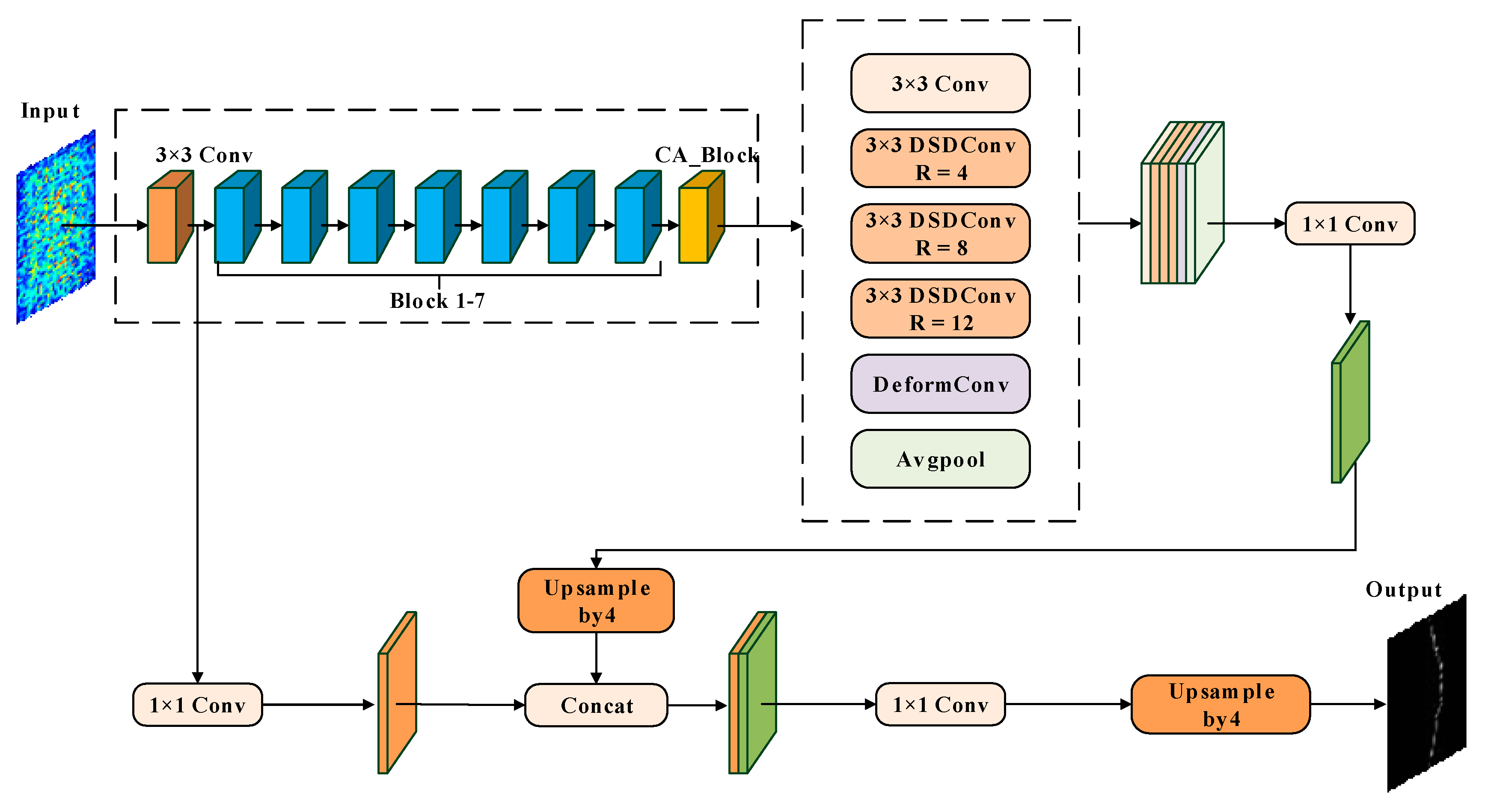
Detection Network of the Photon Count Peak Position

We first used the DeeplabV3+ network to detect the position of the peak photon number in the magnetospheric system of soft X-ray images.

The DeeplabV3+ network includes two stages: encoding and decoding. In the encode phase, feature extraction is first performed through the Xception backbone network. The feature maps extracted from the last layer of the backbone network are sent to the ASPP module for deep feature extraction. The shallow feature map output from the middle layer of the backbone network retains more original feature information and is sent to the decoder. In the decoding stage, a shallow layer was introduced into the feature map through a group of 1 × 1. The convolution is resized and then stacked with a high-level semantic feature output by the ASPP module. After 3 × 3 convolution, the merged feature image was again upsampled four times to output the segmentation result with the same resolution as the original image.

However, in the Encode stage of the DeepLabv3+ semantic segmentation network, the spatial dimension of the target feature map is gradually reduced during the model training process, resulting in the loss of some target features, and detailed recovery cannot be achieved in the decode stage.

We propose a semantic segmentation network model for the magnetospheric system of soft X-ray images based on DeeplabV3+. The improved content includes the following: the backbone network is replaced by the improved network of MobileNetv2, the CA attention module is introduced [45], and ASPP is changed into a multi-branch feature fusion module, introduces deformable convolution, and changes the dilation rate of Atrous Convolution. The improved network structure is shown in Figure 7.

The backbone network was improved by MobileNetv2, including one conv-2D, seven inverted-Rsblock modules, and one CA attention module. The inverted Rsblock module is composed of three conv-2D, two ReLU, and one residual connection, as shown in Figure 8. The size of the convolution kernel is 3 × 3, the padding is 1, and the step size is 1. First, a 1 × 1 convolution is used to increase the dimension of the input feature map, and then a 3 × 3 depthwise convolution is used to perform the convolution operation. Finally, a 1 × 1 convolution operation is used to reduce its dimensions. Instead of using the ReLU activation function, we used a linear activation function to retain more feature information and ensure the expression ability of the model.

The CA module aggregates features from two dimensions of height and width to enhance the positioning of the maximum photon number in the Mobilenetv2 network, obtaining high-level and low-level semantic features of the input feature map. Deep semantic information (30 × 30 × 320) transmits to the feature fusion module, shallow semantic information (128 × 128 × 24) with rich target edge feature information, which is transmitted to the encode stage to retain more global information and is conducive to improving the segmentation accuracy. The CA module structure is shown in Figure 9.

The feature depth was extracted using a multi-branch feature fusion module. It includes one 1 × 1 convolution and three atrous convolutions with dilation rates of 4, 8, and 12, respectively, to obtain different receptive fields and capture multi-scale information. The experiment shows that dilation rates of 4, 8, and 12 are more suitable for feature extraction of the maximum value of the SXI photon number without changing the other conditions. In the ASPP module of the DeepLabv3+ network, the atrous convolution method used in the network increases the receptive field of the input feature map of the backbone network, which is ideal for the extraction of large-size targets, but the extraction effect of small target features such as the maximum photon intensity becomes worse. To improve the expression ability of the model for small targets, in addition to adjusting the dilation rate, a deformable convolution is also introduced to adjust the bias of the sampling position of the feature map according to the current content of the feature map, such that the network is more sensitive to the position of the peak photon number, and targets with small solar wind density can be detected and segmented more accurately. Finally, a global average pooling module is used to overcome the problem of effective weight reduction at long distances. We then stacked the characteristic diagrams of each branch, as shown in Equations (3)–(9). Subsequently, through a 1 × 1 convolution integration feature, we obtained a feature map with a size of 32 × 32 × 256.

$$\mathrm{X}1=\mathrm{conv}1\times 1\left(\mathrm{x}\right)$$

(3)

$$\mathrm{X}2=\mathrm{conv}3\times 3\_1\left(\mathrm{x}\right)$$

(4)

$$\mathrm{X}3=\mathrm{conv}3\times 3\_2\left(\mathrm{x}\right)$$

(5)

$$\mathrm{X}4=\mathrm{conv}3\times 3\_3\left(\mathrm{x}\right)$$

(6)

$$\mathrm{X}4=\mathrm{DeformConv}\left(\mathrm{x}\right)$$

(7)

$$\mathrm{X}5=\mathrm{Global}\_\mathrm{feature}\left(\mathrm{x}\right)$$

(8)

$$\mathrm{x}=\mathrm{X}1+\mathrm{X}2+\mathrm{X}3+\mathrm{X}4+\mathrm{X}5$$

(9)

where x is the input signal, X is the final output feature map of the multi-branch feature fusion module, X1 is the characteristic diagram of the 1 × 1 convolution branch output, X2 is the characteristic diagram of the atrous convolution branch output with a dilation rate of 4, X3 is the characteristic diagram of the atrous convolution branch output with a dilation rate of 8, X4 is the characteristic diagram of the atrous convolution branch output with a dilation rate of 12, and conv3 × 3_1(x), conv3 × 3_2(x), and conv3 × 3_3(x) represent void convolution operations with void rates of 4, 8, and 12, respectively.

Loss Function

The loss function uses the binary cross-entropy loss function, as shown in Equation (10), where N is the number of samples, y_i is tag 0 or 1, and p_i is the predicted value.

$$\mathrm{Loss}=-{\displaystyle \sum }_{\mathrm{i}=1}^{\mathrm{N}}\left({\mathrm{y}}_{\mathrm{i}}{\mathrm{lgp}}_{\mathrm{i}}+\left(1-{\mathrm{y}}_{\mathrm{i}}\right)\lg \left(1-{\mathrm{p}}_{\mathrm{i}}\right)\right)$$

(10)

Model Training

The training process included two stages: freezing and thawing. During the freezing stage, the backbone of the model was frozen, the feature extraction network did not change, and the occupied video memory was small. Only the network was fine-tuned. The batch size was eight, and the epoch was 50. In the unfreezing stage, the backbone of the model is not frozen and the feature extraction network changes. The batch size was four, and the total epoch was 100.

Accuracy Evaluation Metrics

In this study, the pixel accuracy (PA) was taken as the evaluation index, as shown in (11).

$$\mathrm{Pixel}\mathrm{Accuracy}=\frac{{{\displaystyle \sum }}_{\mathrm{i}=0}^{\mathrm{k}}{\mathrm{p}}_{\mathrm{ii}}}{{{\displaystyle \sum }}_{\mathrm{i}=0}^{\mathrm{k}}{{\displaystyle \sum }}_{\mathrm{j}=0}^{\mathrm{k}}{\mathrm{p}}_{\mathrm{ij}}}$$

(11)

where k is the category, ${\mathrm{p}}_{\mathrm{ii}}$ is the number of correctly predicted pixels, and ${\mathrm{p}}_{\mathrm{ij}}$ is the total number of pixels. The average pixel accuracy is used to calculate the proportion of the number of correctly classified pixels of each class separately and then accumulated to calculate the average.

2.2.3. Magnetopause Position Detection

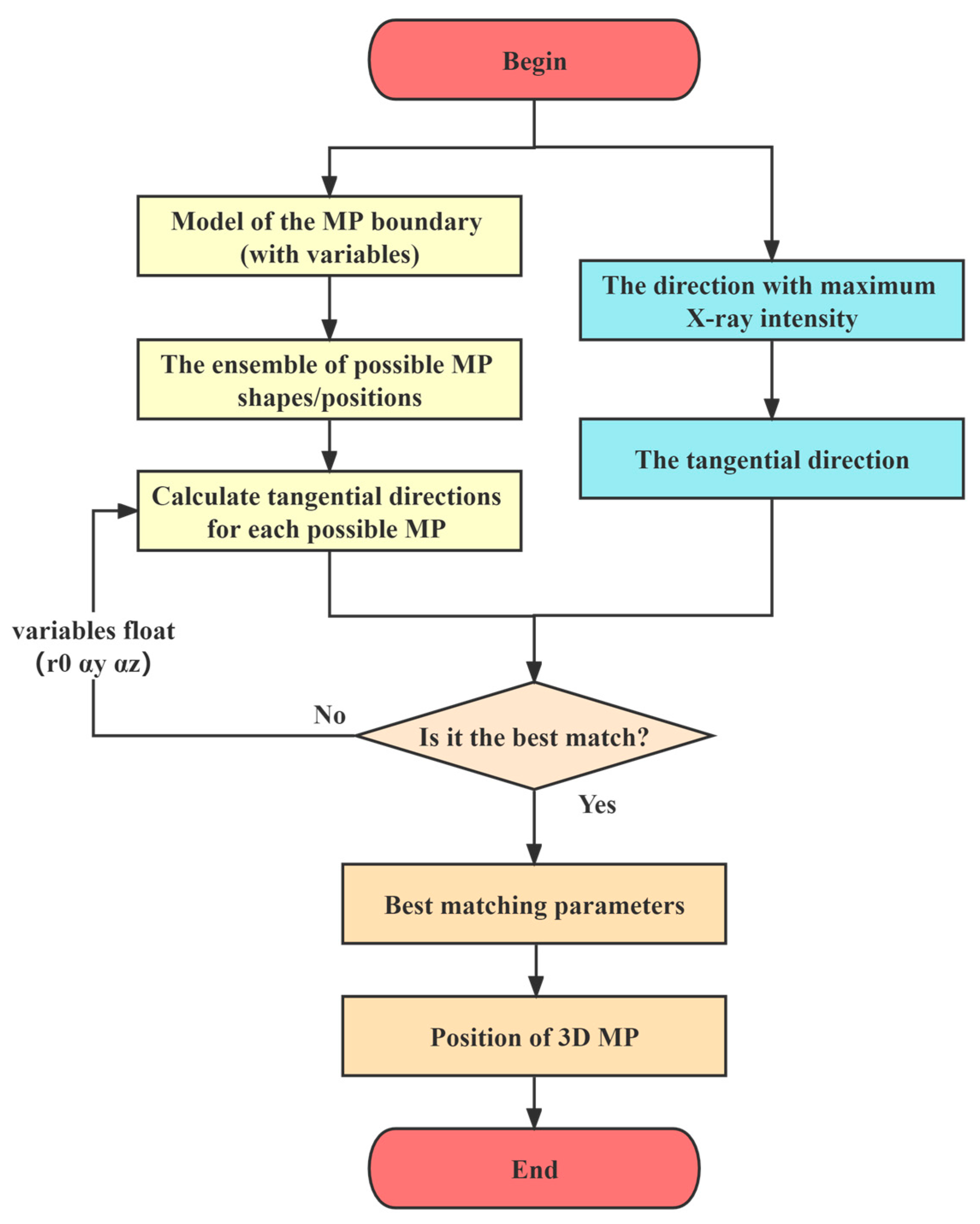
TFA Calculation Model

In this study, the tangent fitting approach (TFA) was used to retrieve the 3D magnetopause position from 2D images. The TFA flow is shown in Figure 10. Previous studies have shown that the tangent to the magnetopause is at the maximum X-ray intensity [20] or located between the maximum X-ray intensity gradient and the maximum emissivity, probably closer to the maximum X-ray intensity gradient [23]. New research shows that the maximum soft X-ray intensity gradient tends to be the tangent of the magnetopause’s inner boundary, while the maximum soft X-ray intensity tends to be the tangent of the magnetopause’s outer boundary [46]. This paper assumes that the location of the maximum pixel point of X-ray intensity corresponds to the tangential direction of the magnetopause in order to simplify the calculation.

Then, the magnetopause boundary model was constructed, and the expression of the magnetopause boundary model in the solar magnetospheric coordinate system (GSM) was as follows:

$$\mathrm{r}\left(\mathsf{\theta },\mathsf{\varphi }\right)=\frac{{\mathrm{r}}_{\mathrm{y}}\left(\mathsf{\theta }\right){\mathrm{r}}_{\mathrm{z}}\left(\mathsf{\theta }\right)}{\sqrt{{\left[{\mathrm{r}}_{\mathrm{z}}\left(\mathsf{\theta }\right)\cos \mathsf{\varphi }\right]}^2+{\left[{\mathrm{r}}_{\mathrm{y}}\left(\mathsf{\theta }\right)\sin \mathsf{\varphi }\right]}^2}}$$

(12)

where θ is the angle between the r and x axes, and ϕ is the rotation angle between the y axis and the projection of r in the y-z plane. The expressions for r_y and r_z are:

$${\mathrm{r}}_{\mathrm{y}}\left(\mathsf{\theta }\right)={\mathrm{r}}_0{\left(\frac{2}{1+\cos \mathsf{\theta }}\right)}^{{\mathsf{\alpha }}_{\mathrm{y}}}$$

(13)

$${\mathrm{r}}_{\mathrm{z}}\left(\mathsf{\theta }\right)={\mathrm{r}}_0{\left(\frac{2}{1+\cos \mathsf{\theta }}\right)}^{{\mathsf{\alpha }}_{\mathrm{z}}}$$

(14)

By changing the variable parameters r₀, α_y, and α_z, we obtained a series of magnetopause configurations, calculated the tangential directions of each possible configuration, and compared them with the tangential directions obtained from the X-ray image to find the most matching set of parameters. Finally, the configuration of the 3D magnetopause was obtained via inversion of the most matched set of parameters.

Accuracy Evaluation Metrics

In this study, we use the position error $∆{\mathrm{r}}_0$ of the subsolar point of the magnetopause as the evaluation index for magnetopause detection.

$$∆{\mathrm{r}}_0=\left|{\mathrm{r}}_0^{\prime }-{\mathrm{r}}_0\right|$$

(15)

where ${\mathrm{r}}_0^{\prime }$ is the position of the subsolar magnetopause calculated from the SXI image and ${\mathrm{r}}_0$ is the position of the subsolar magnetopause calculated from the MHD image.

3. Results

3.1. Detection of the Photon Count Peak Position

Figure 11 shows the detection results of the maximum photon counts of the SXI simulation image with an integration time of 30 s under a uniform cosmic background using the traditional method, the MHD, and our network. The maximum value of the MHD intensity is the source of the data untag and can be used as a reference for “true value”. The traditional method involves obtaining the maximum value for each row of the SXI simulation image. The smaller the solar wind density, the more scattered the detection results are. When the solar wind density N = 5 cm⁻³, the detection results spread all over the entire image. The network detection results proposed in this study were concentrated and fit well with the maximum value of the MHD radiation intensity.

Figure 12 shows the detection efficiency of the network on three types of noise background with integration times of 30, 60, 120, and 240 s, respectively. The data without background noise showed the lowest accuracy of 86.28% at the lowest integration time of 30 s and the highest accuracy of 94.44% at 240 s. Similarly, when testing data with uniform and non-uniform cosmic background noise, the detection accuracy is lowest at the shortest integration time and highest at the minimum integration time. The PA of SXI simulation images with uniform cosmic background noise and integration times of 30, 60, 120, and 240 s was 78.87%, 92.3%, 95.31%, and 95.85%, respectively.

Figure 13 shows the detection efficiency of the network on three noise backgrounds with solar wind density 5 cm⁻³, 12 cm⁻³, 20 cm⁻³, and 30 cm⁻³. The data without background noise showed the lowest accuracy of 92.8% at the lowest solar wind density N = 5, and the highest accuracy at N = 30 at 95.47%. Similarly, the data of uniform cosmic background noise have the lowest accuracy at the minimum solar wind density and the highest accuracy at the maximum solar wind density. The PA of SXI simulation images with uniform cosmic background noise and solar wind number density of 5 cm⁻³, 12 cm⁻³, 20 cm⁻³, and 30 cm⁻³ was 78.87%, 92.3%, 95.31%, and 95.85%, respectively.

We also compared the detection efficiency before and after the network improvement and the detection result of the SXI image with uniform cosmic background noise. The PA increased from 56.9% to 90.94%. Compared with the original network deeplabv3+, the network proposed in this paper improves the deep feature extraction method of the target in the Encode stage and improves the detection ability of the network for the maximum photon intensity of the magnetospheric system with low solar wind density.

3.2. Magnetopause Position Detection

Taking the detection result of the maximum photon intensity of the magnetosphere system as the input to TFA, the calculation result of TFA is as shown in Figure 14. Using the calculation results of the MHD as a reference, the magnetopause configuration obtained using the traditional method does not match the MHD calculation results at the solar wind density N = 5 cm⁻³ and N = 12 cm⁻³ for all the considered exposure time, and the magnetopause configuration is similar to the MHD when the solar wind density N = 20 cm⁻³ and N = 30 cm⁻³ but there are certain errors with shorter exposure time. The magnetopause configuration obtained using our method can be approximately the same as that of the MHD, even when the solar wind density is N = 5 cm⁻³.

The calculation results for r₀ at different integration times and solar wind number densities are listed in

Table 2. The calculation unit of r₀ in different integration time and different solar wind number density is: (R_E).

Solar Wind Density	MHD	30 s		60 s		120 s		240 s
		Traditional	Ours	Traditional	Ours	Traditional	Ours	Traditional	Ours
5	10.15	6	10.25	8.65	10.2	6	10.15	8.85	10.15
12	9.2	6	9.3	6	9.3	6	9.35	8.85	9.35
20	8.4	8.3	8.4	8.35	8.4	8.35	8.45	8.5	8.4
30	7.7	8.1	7.8	8.1	7.9	8.05	7.9	7.95	7.8

. Figure 15 shows the test data with uniform cosmic background noise. Taking the position error $∆$r₀ of the magnetopause as the evaluation standard, the magnetopause detection results under different solar wind number densities with integration times of 30 s, 60 s, 120 s, and 240 s are shown. The $∆$r₀ of the traditional method is greater than 1R_E for the data of 30 s, 60 s, 120 s, and 240 s when the solar wind density N = 5 cm⁻³. The minimum r₀ of the test data was 0 and the maximum was 0.2R_E.

4. Discussion

The proposed method is beneficial in SXI image detection with different integration times and solar wind densities. The longer the integration time and the larger the solar wind number density is, the better the detection efficiency of the photon number maximum position will be. Because the network learns more spatial features and improves the sensitivity to weak signals, the detection of shorter integration times and lower solar wind number density is significantly improved compared with traditional methods. In fact, after processing, the final magnetopause configuration was close to the “truth”, and the position error of the subsolar magnetopause was within the instrument error range. The specific analysis is as follows.

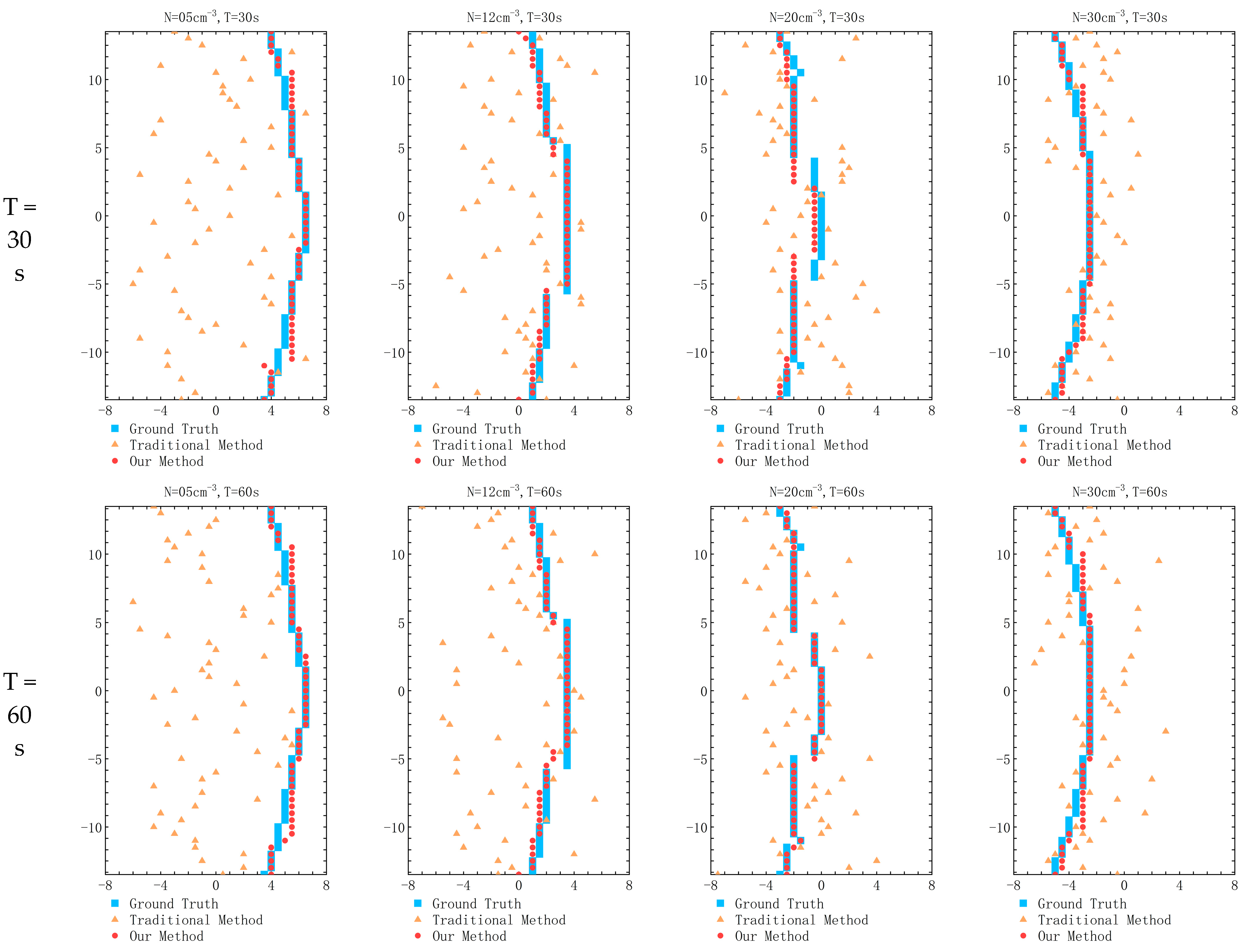
4.1. SXI Images Detection for Different Integration Times

As shown in Figure 13, under the test set with different background noises, PA increased as the integration time increased. When the integration time was 30 s, the network had the best detection efficiency on the test set with no background noise, and the PA reached 86.28%. When the integration time was 60, 120, and 240 s, the network had a slightly higher detection efficiency on the test set with uniform noise than on the test set with no background noise and the test set with non-uniform background noise. This is because the signal strength is low when the integration time is short, the background noise is equivalent to the target signal strength, and the background noise has a significant impact on the detection performance. As the integration time increases, the target signal strength increases and the influence of background noise decreases, so the detection efficiency of the network on the three types of backgrounds is not different.

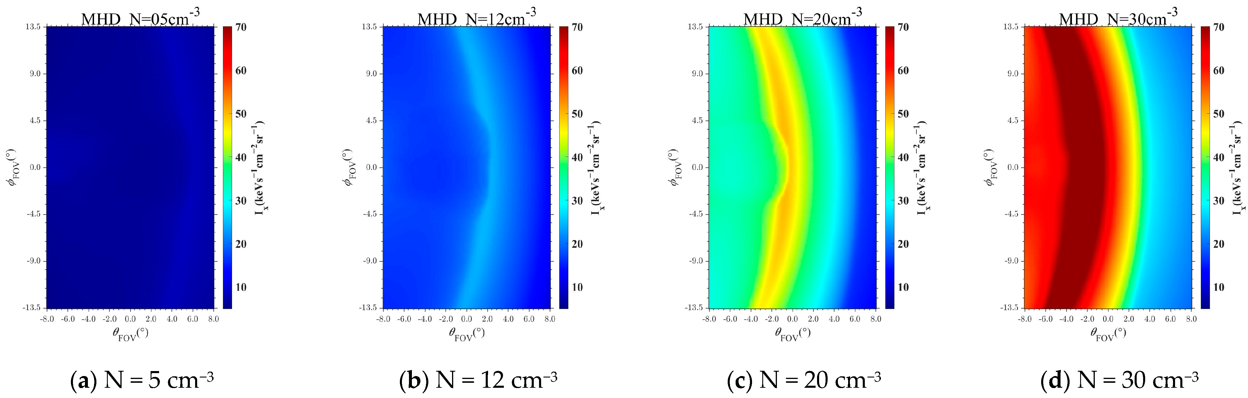
4.2. SXI Image Detection for Different Solar Wind Densities

It can be seen from Figure 13 that, for all kinds of background noise test sets, PA increases with an increase in solar wind density. When the solar wind density is 5cm⁻³, the network had the best detection efficiency on the test set with no background noise, with a PA of 92.8%. When the solar wind density was 20 cm⁻³ and 30 cm⁻³, the network had a slightly higher detection efficiency on the test set with uniform noise than on the test set with no background and with nonuniform background noise. This is because solar wind density is proportional to the target signal intensity. When the solar wind particle number density is small, the X-ray radiation rate is not large enough, and the light source that can be detected by the instrument is not strong enough, resulting in the amplification of the impact of cosmic background and instrument noise on the results. With the increase in the number density of solar wind particles and the increase in the X-ray radiation rate, the instrument can detect more light sources and reduce the impact of noise, so the detection efficiency of the network on the three types of background was not different.

4.3. Magnetopause Position Detection

Because the pixel size of SXI is approximately 0.5°, it corresponds to a spatial accuracy of approximately 0.2RE on a spatial scale [22]. The calculation results of TFA in 3.2 show that the traditional method of detecting the position of the magnetopause is closer to the ‘true value’ with the increase in the integration time, but the noise effect is too large when the solar wind density is small, and the increase in the integration time cannot completely compensate for the noise of the film and television. When N = 5 cm⁻³, Δr₀ is always greater than 1. The results of this research method, Δr₀, for different integration times and different solar wind density ranges did not exceed the instrument error and met the detection requirements.

5. Conclusions

We proposed a detection network of maximum photon counts in the magnetospheric system based on deep learning, which was used to detect the pixel position of the maximum magnetospheric system photon intensity, and then obtained the magnetopause 3D configuration through TFA calculation. Taking the MHD integral image and SXI simulation image of the magnetosphere system as the data source, we extracted the position of the maximum photon intensity pixel of the magnetosphere system under different solar wind densities from the improved network of deeplabv3+ and obtained the position of the magnetopause via TFA. Comparing the detection results of the SXI simulation image with the traditional method, the results show that our model can detect the maximum pixel position of photon intensity in the absence of cosmic background noise and the presence of cosmic background noise, especially in the magnetospheric system with low solar wind density that the traditional method cannot achieve. The minimum exposure time required for a single test is only 30 s, which is ten-times shorter than the traditional method. At the same time, compared to the “true value” of the magnetopause configuration calculated via TFA using the detection results as input, our method has a smaller error than that of the traditional method. However, the real-time performance of our model requires further improvement. Future work will focus on the comprehensive consideration of accuracy, complexity, and reasoning speed, so that the model can consider high accuracy, light weight, and effectiveness at the same time.

References

1. Wang, C.; Li, Z.J.; Sun, T.R.; Liu, Z.Q.; Liu, J.; Wu, Q.; Zheng, J.H.; Li, J. SMILE Satellite mission survey. Space Int. 2017, 464, 13–16. (In Chinese) [Google Scholar]
2. Branduardi-Raymont, G.; Escoubet, C.P.; Kuntz, K.; Lui, T.; Read, A.; Sibeck, D.; Dai, L.; Dmitriev, A.; Donovan, E.; Dunlo, M.; et al. Link between Solar Wind, Magnetosphere, and Lonosphere. ISSI-BJ Magazine, 27 January 2016; p. 9. [Google Scholar]
3. Sonett, C.P.; Abrams, I.J. The distant geomagnetic field: 3. Disorder and shocks in the magnetopause. J. Geophys. Res. 1963, 68, 1233–1263. [Google Scholar] [CrossRef]
4. Cahill, L.J.; Amazeenp, G. The boundary of the geo-magnetic field. J.Geophys. Res. 1963, 68, 1835–1843. [Google Scholar] [CrossRef]
5. Lisse, C.M.; Dennerl, K.; Englhauser, J.; Harden, M.; Marshall, F.E.; Mumma, M.J.; Petre, R.; Pye, J.P.; Ricketts, M.J.; Schmitt, J.H.; et al. Discovery of X-ray and extreme ultraviolet emission from comet C/Hyakutake 1996 B2. Science 1996, 274, 205–209. [Google Scholar] [CrossRef]
6. Kuntz, K.D.; Collado-Vega, Y.M.; Collier, M.R.; Connor, H.; Cravens, T.E.; Koutroumpa, D.; Porter, F.; Robertson, I.P.; Sibeck, D.G.; Snowden, S.L.; et al. The solar wind charge-exchange production factor for hydrogen. Rev. Sci. Instrum. 2015, 808, 143. [Google Scholar] [CrossRef]
7. Robertson, I.P.; Collier, M.R.; Cravens, T.E.; Fok, M.-C. X-ray emission from the terrestrial magnetosheath including the cusps. J. Geophys. Res. Atmos. 2006, 111, Al2105. [Google Scholar] [CrossRef]
8. Dennerl, K. High Resolution X-ray Spectroscopy of Comets. In Proceedings of the International Workshop, London, UK, 19 March 2009. [Google Scholar]
9. Schwadron, N.A.; Cravens, T.E. Implications of solar wind composition for cometary X-rays. Astrophys. J. 2000, 544, 558–566. [Google Scholar] [CrossRef]
10. Carter, J.A.; Sembay, S. Identifying XMM-Newton observations affected by solar wind charge exchange—Part I. Astron. Astrophys. 2008, 489, 837–848. [Google Scholar] [CrossRef]
11. Carter, J.A.; Sembay, S.; Read, A.M. A high charge state coronal mass ejection seen through solar wind charge exchange emission as detected by XMM-Newton. Mon. Not. R. Astron. Soc. 2010, 402, 867. [Google Scholar] [CrossRef]
12. Carter, J.A.; Sembay, S.; Read, A.M. Identifying XMM-Newton observations affected by solar wind charge exchange—Part II. Astron. Astrophys. 2011, 527, A115. [Google Scholar] [CrossRef]
13. Fujimoto, R.; Mitsuda, K.; McCammon, D.; Takei, Y.; Bauer, M.; Ishisaki, Y.; Porter, F.S.; Yamaguchi, H.; Hayashida, K.; Yamasaki, N.Y. Evidence for solar-wind charge-exchange X-ray emission from the Earth’s magnetosheath. Publ. Astron. Soc. Jpn. 2007, 59, 133–140. [Google Scholar] [CrossRef]
14. Snowden, S.L.; Collier, M.R.; Cravens, T.; Kuntz, K.D.; Lepri, S.T.; Robertson, I.; Tomas, L. Observation of solar wind charge exchange emission from exospheric material in and outside Earth’s magnetosheath 2008 September 25. Astrophys. J. 2009, 691, 372–381. [Google Scholar] [CrossRef]
15. Sun, T.R.; Wang, C.; Sembay, S.F.; Lopez, R.E.; Escoubet, C.P.; Branduardi-Raymont, G.; Zheng, J.H.; Yu, X.Z.; Guo, X.C.; Dai, L.; et al. Soft X-ray Imaging of the Magnetosheath and Cusps Under Different Solar Wind Conditions: MHD Simulations. J. Geophys. Res. Space Phys. 2019, 124, 2435–2450. [Google Scholar] [CrossRef]
16. Samsonov, A.; Carter, J.A.; Read, A.; Sembay, S.; Branduardi-Raymont, G.; Sibeck, D.; Escoubet, P. Finding Magnetopause Standoff Distance using a Soft X-ray Imager–Part 1, Magnetospheric masking. J. Geophys. Res. Space Phys. 2022, 127, e2022JA030848. [Google Scholar]
17. Peng, S.; Ye, Y.; Wei, F.; Yang, Z.; Guo, Y.; Sun, T. Numerical model built for the simulation of the earth magnetopause by lobster-eye-type soft X-ray imager onboard SMILE satellite. Opt. Express. 2018, 26, 15138–15152. [Google Scholar] [CrossRef]
18. Jorgensen, A.M.; Sun, T.; Wang, C.; Dai, L.; Sembay, S.; Wei, F.; Guo, Y.; Xu, R. Boundary Detection in Three Dimensions with Application to the SMILE Mission: The Effect of Photon Noise. J. Geophys. Res. Space Phys. 2019, 124, 4365–4383. [Google Scholar] [CrossRef]
19. Jorgensen, A.M.; Sun, T.; Wang, C.; Dai, L.; Sembay, S.; Zheng, J.; Yu, X. Boundary Detection in Three Dimensions with Application to the SMILE Mission: The Effect of Model-Fitting Noise. J. Geophys. Res. Space Phys. 2019, 124, 4341–4355. [Google Scholar] [CrossRef]
20. Collier, M.R.; Connor, H.K. Magnetopause Surface Reconstruction from Tangent Vector Observations. J. Geophys. Res. Space Phys. 2018, 123, 10189–10199. [Google Scholar] [CrossRef]
21. Sun, T.; Wang, C.; Connor, H.K.; Jorgensen, A.M.; Sembay, S. Deriving the Magnetopause Position from the Soft X-ray Image by Using the Tangent Fitting Approach. J. Geophys. Res. Space Phys. 2020, 125, e28169. [Google Scholar] [CrossRef]
22. Guo, Y.; Sun, T.; Wang, C.; Sembay, S. Deriving the magnetopause position from wide field-of-view soft X-ray imager simulation. Sci. China Earth Sci. 2022, 65, 1601–1611. [Google Scholar] [CrossRef]
23. Samsonov, A.; Carter, J.A.; Read, A.; Sembay, S.; Branduardi-Raymont, G.; Sibeck, D.; Escoubet, P. Finding Magnetopause Standoff Distance using a Soft X-ray Imager–Part 2, Methods to Analyze 2-DX-ray Images. J. Geophys. Res. Space Phys. 2022, 127, e2022JA030850. [Google Scholar]
24. Long, J.; Shelhamer, E.; Darrell, T. Fully Convolutional Networks for Semantic Segmentation. In Proceedings of the 2015 IEEE Conference on Computer Vision and Pattern Recognition, Boston, MA, USA, 7–12 June 2015; pp. 3431–3440. [Google Scholar]
25. Ronneberger, O.; Fischer, P.; Brox, T. U-Net: Convolutional Networks for Biomedical Image Segmentation. In Proceedings of the International Conference on Medical Image Computing and Computer Assisted Intervention, Munich, Germany, 5–9 October 2015; pp. 234–241. [Google Scholar]
26. Badrinarayanan, V.; Kendall, A.; Cipolla, R. SegNet: A Deep convolutional encoder-decoder architecture for image segmentation. IEEE Trans. Pattern Anal. Mach. Intell. 2017, 39, 2481–2495. [Google Scholar] [CrossRef] [PubMed]
27. Zhao, H.; Shi, J.; Qi, X.; Wang, X.; Jia, J. Pyramid scene parsing network. In Proceedings of the 2017 IEEE Conference on Computer Vision and Pattern Recognition, Honolulu, HI, USA, 21–26 July 2017; pp. 2881–2890. [Google Scholar] [CrossRef]
28. Howard, A.G.; Zhu, M.; Chen, B.; Kalenichenko, D.; Wang, W.; Weyand, T.; Andreetto, M.; Adam, H. Mobile Nets: Efficient convolutional neural networks for mobile vision applications. arXiv 2017, arXiv:1704.04861. [Google Scholar]
29. Sandler, M.; Howard, A.; Zhu, M.; Zhmoginov, A.; Chen, L.C. MobileNetV 2, Inverted Residuals and Linear Bottlenecks. In Proceedings of the 2018 IEE Conference on Computer Vision and Pattern Recognition, Salt Lake City, UT, USA, 18–23 June 2018; pp. 4510–4520. [Google Scholar]
30. Chen, L.C.; Papandreou, G.; Kokkinos, I.; Murphy, K.; Yuille, A.L. Semantic Image Segmentation with Deep Convolutional Nets and Fully Connected CRFs. arXiv 2014, arXiv:1412.7062. [Google Scholar]
31. Simonyan, K.; Zisseman, A. VeryDeep Convolutional Net-works for Large-scale Image Recognition [EB/OL]. arXiv 2014, arXiv:1409.1556. [Google Scholar]
32. Chen, L.C.; Papandreou, G.; Kokkinos, I.; Murphy, K.; Yuille, A.L. Deeplab: Semantic image segmentation with deep convolutional nets, atrous convolution, and fully connected crfs. arXiv 2016, arXiv:1606.00915. [Google Scholar] [CrossRef]
33. Chen, L.C.; Papandreou, G.; Schroff, F.; Adam, H. Rethinking atrous convolution for semantic image segmentation. arXiv 2017, arXiv:1706.05587. [Google Scholar]
34. Chen, L.C.; Zhu, Y.; Papandreou, G.; Schroff, F.; Adam, H. Encoder-Decoder with Atrous Separable Convolution for Semantic Image Segmentation. In Proceedings of the European Conference on Computer Vision (ECCV), Munich, Germany, 8–14 September 2018; pp. 833–851. [Google Scholar]
35. Wang, J.; Liu, X. Medical image recognition and segmentation of pathological slices of gastric cancer based on Deeplab v3+ neural network. Comput. Methods Programs Biomed. 2021, 207, 106210. [Google Scholar] [CrossRef]
36. Shoushtari, F.K.; Sina, S.; Dehkordi, A.N. Automatic segmentation of glioblastoma multiform brain tumor in MRI images: Using Deeplabv3+ with pre-trained Resnet18 weights. Phys. Med. 2022, 100, 51–63. [Google Scholar] [CrossRef]
37. Jung, Y.J.; Kim, M.J. Deeplab v3+ Based Automatic Diagnosis Model for Dental X-ray: Preliminary Study. J. Magn. 2020, 25, 632–638. [Google Scholar] [CrossRef]
38. Hu, Y.Q.; Guo, X.C.; Wang, C. On the ionospheric and reconnection potentials of the Earth: Results from global MHD simulations. J. Geophys. Res. 2007, 112, A07215. [Google Scholar] [CrossRef]
39. Cravens, T.E. Comet Hyakutake X-ray source: Charge transfer of solar wind heavy ions. Geophys. Res. Lett. 1997, 100, 24105–24108. [Google Scholar] [CrossRef]
40. Zhang, Y.; Sun, T.; Carter, J.A.; Sembay, S.; Koutroumpa, D.; Ji, L.; Liu, W.; Wang, C. Dynamical response of solar wind charge exchange soft X-ray emission in Earth’s magnetosphere to the solar wind proton flux. Astrophys. J. 2023, 948, 69. [Google Scholar] [CrossRef]
41. Cravens, T.E. Heliospheric X-ray Emission Associated with Charge Transfer of the Solar Wind with Interstellar Neutrals. Astrophys. J. 2000, 532, L153–L156. [Google Scholar] [CrossRef]
42. Cravens, T.E.; Robertson, I.P.; Snowden, S.L. Temporal variations of geocoronal and heliospheric X-ray emission associated with the solar wind interaction with neutrals. J. Geophys. Res. 2001, 106, 24883–24892. [Google Scholar] [CrossRef]
43. Sun, T.R.; Wang, C.; Wei, F.; Sembay, S. X-ray imaging of Kelvin-Helmholtz waves at the magnetopause. J. Geophys. Res. Space Phys. 2015, 120, 266–275. [Google Scholar] [CrossRef]
44. Sun, T.; Wang, X.; Wang, C. Tangent directions of the cusp boundary derived from the simulated soft X-ray image. J. Geophys. Res. Space Phys. 2021, 126, e28314. [Google Scholar] [CrossRef]
45. Hou, Q.; Zhou, D.; Feng, J. Coordinate attention for efficient mobile network design. In Proceedings of the IEEE/CVF Conference on Computer Vision and Pattern Recognition, Nashville, TN, USA, 21 June 2021; pp. 13713–13722. [Google Scholar]
46. Zhang, Y.; Sun, T.; Carter, J.A.; Liu, W.; Sembay, S.; Ji, L.; Wang, C. The Relationship between Solar Wind Charge Exchange Soft X-ray Emission and the Tangent Direction of Magnetopause in an XMM–Newton Event. Magnetochemistry 2023, 9, 88. [Google Scholar] [CrossRef]
Figure 1. MHD 2D integral diagrams: (a) N = 5 cm−3; (b) N = 12 cm−3; (c) N = 20 cm−3; (d) N = 30 cm−3.
Remotesensing 15 02771 g001
Figure 2. SXI simulation diagram with an integration time of 30 s: (a) N = 5 cm−3; (b) N = 12 cm−3; (c) N = 20 cm−3; (d) N = 30 cm−3.
Remotesensing 15 02771 g002
Figure 3. SXI simulation images with different integration times: (a) N = 5 cm−3; (b) N = 12 cm−3; (c) N = 20 cm−3; (d) N = 30 cm−3.
Remotesensing 15 02771 g003
Figure 4. MHD integration images and SXI simulation images with different backgrounds.
Remotesensing 15 02771 g004aRemotesensing 15 02771 g004b
Figure 5. Target labeling: (a) N = 5 cm−3; (b) N = 12 cm−3; (c) N = 20 cm−3; (d) N = 30 cm−3.
Remotesensing 15 02771 g005
Figure 6. Magnetopause detection flow chart.
Remotesensing 15 02771 g006
Figure 7. Network structure.
Remotesensing 15 02771 g007
Figure 8. Inverted Rsblock module structure diagram.
Remotesensing 15 02771 g008
Figure 9. CA module structure diagram.
Remotesensing 15 02771 g009
Figure 10. TFA flow chart.
Remotesensing 15 02771 g010
Figure 11. Photon number maximum position detection results.
Remotesensing 15 02771 g011aRemotesensing 15 02771 g011b
Figure 12. Detection results of different integration times.
Remotesensing 15 02771 g012
Figure 13. Detection results of different solar wind densities.
Remotesensing 15 02771 g013
Figure 14. Calculation results of magnetopause configuration.
Remotesensing 15 02771 g014aRemotesensing 15 02771 g014b
Figure 15. The calculation results of  r0 at different integration times, with t = 30, 60, 120, and 240 s from top to bottom.
Remotesensing 15 02771 g015aRemotesensing 15 02771 g015b