

Upper Mantle Velocity Structure Beneath the Yarlung–Tsangpo Suture Revealed by Teleseismic P-Wave Tomography


Abstract
:
1. Introduction
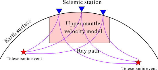
2. Data and Method
3. Results and Discussion
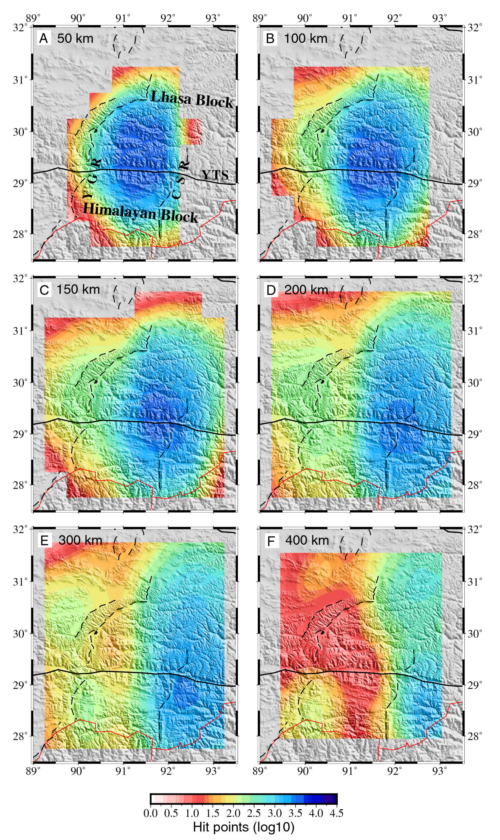
3.1. Ray Path Coverage
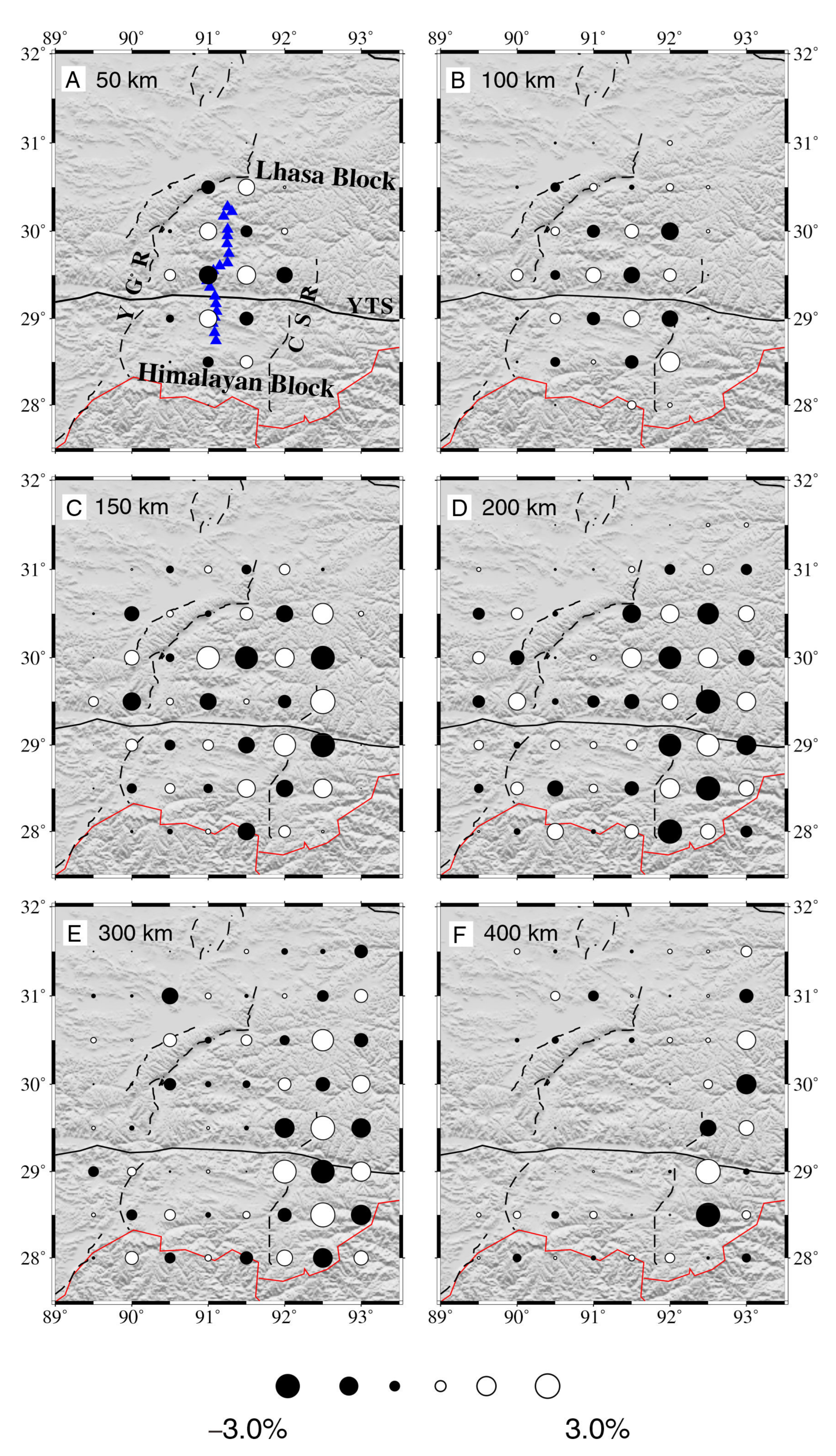
3.2. Checkerboard Resolution Tests
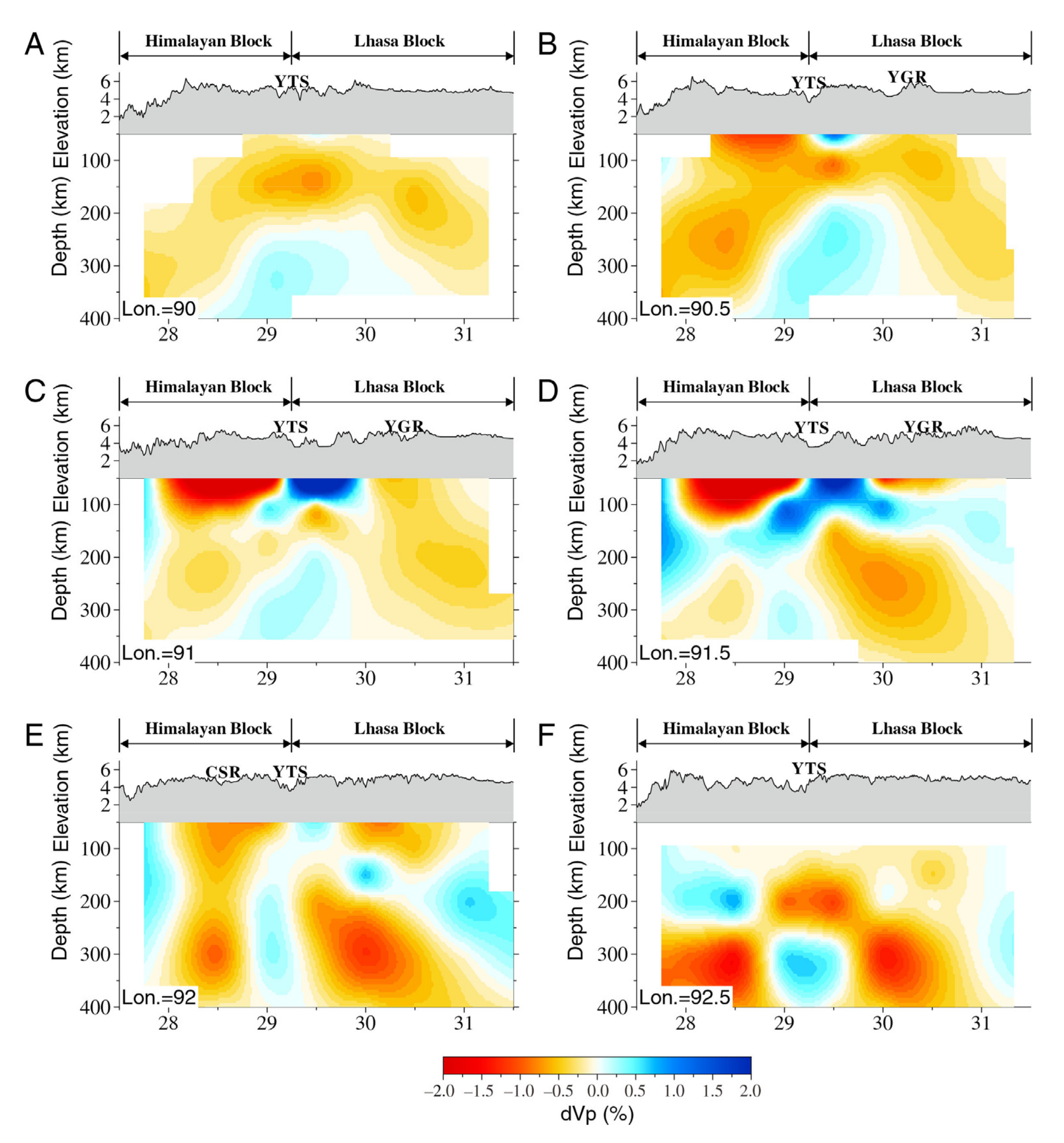
3.3. Tomographic Imaging
3.4. Restoring Resolution Tests
3.5. Tectonic Implications
4. Conclusions
Supplementary Materials
Author Contributions
Funding
Data Availability Statement
Acknowledgments
Conflicts of Interest
References
- Yin, A.; Harrison, T.M. Geologic evolution of the Himalayan-Tibetan orogen. Annu. Rev. Earth Planet. Sci. 2000, 28, 211–280. [Google Scholar] [CrossRef]
- Royden, L.H.; Burchfiel, B.C.; van der Hilst, R.D. The geological evolution of the Tibetan plateau. Science 2008, 321, 1054–1058. [Google Scholar] [CrossRef] [PubMed]
- Tapponnier, P.; Peltzer, G.; Dain, A.Y.L.; Armijo, R.; Cobbold, P. Propagating extrusion tectonics in Asia: New insights from simple experiments with plasticine. Geology 1982, 10, 611–616. [Google Scholar] [CrossRef]
- England, P.; Houseman, G. Finite strain calculations of continental deformation: Comparison with the India-Asia collision zone. J. Geophys. Res. 1986, 91, 3664–3676. [Google Scholar] [CrossRef]
- Royden, L.H.; Burchfiel, B.C.; King, R.W.; Wang, E.; Chen, Z.L.; Shen, F.; Liu, Y. Surface deformation and lower crustal flow in eastern Tibet. Science 1997, 276, 788–790. [Google Scholar] [CrossRef] [PubMed]
- Kind, R.; Yuan, X.; Saul, J.; Nelson, D.; Sobolev, S.V.; Mechie, J.; Zhao, W.; Kosarev, G.; Ni, J.; Achauer, U.; et al. Seismic images of crust and upper mantle beneath Tibet: Evidence for Eurasian plate subduction. Science 2002, 298, 1219–1221. [Google Scholar] [CrossRef] [PubMed]
- Molnar, P.; England, P.; Martinod, J. Mantle dynamics, uplift of the Tibetan Plateau, and the Indian Monsoon. Rev. Geophys. 1993, 31, 357–396. [Google Scholar] [CrossRef]
- Burg, J.; Chen, G. Tectonics and structural zonation of southern Tibet, China. Nature 1984, 311, 219–223. [Google Scholar] [CrossRef]
- Tapponnier, P.; Peltzer, G.; Armijo, R. On the mechanics of the collision between India and Asia. Geol. Soc. Lond. Spec. Publ. 1986, 19, 113–157. [Google Scholar] [CrossRef]
- Turner, S.; Hawkesworth, C.; Liu, J.; Rogers, N.; Kelley, S.; van Calsteren, P. Timing of Tibetan uplift constrained by analysis of volcanic rocks. Nature 1993, 364, 50–54. [Google Scholar] [CrossRef]
- Chung, S.-L.; Lo, C.-H.; Lee, T.-Y.; Zhang, Y.; Xie, Y.; Li, X.; Wang, K.-L.; Wang, P.-L. Diachronous uplift of the Tibetan plateau starting 40?Myr ago. Nature 1998, 394, 769–773. [Google Scholar] [CrossRef]
- Chung, S.-L.; Liu, D.; Ji, J.; Chu, M.-F.; Lee, H.-Y.; Wen, D.-J.; Lo, C.-H.; Lee, T.-Y.; Qian, Q.; Zhang, Q. Adakites from continental collision zones: Melting of thickened lower crust beneath southern Tibet. Geology 2003, 31, 1021–1024. [Google Scholar] [CrossRef]
- Turner, S.; Arnaud, N.; Liu, J.; Rogers, N.; Hawkesworth, C.; Harris, N.; Kelley, S.; van Calsteren, P.; Deng, W. Post-collisional, shoshonitic volcanism on the Tibetan plateau: Implications for convective thinning of the lithosphere and the source of ocean island basalts. J. Petrol. 1996, 37, 45–71. [Google Scholar] [CrossRef]
- Chung, S.-L.; Chu, M.-F.; Zhang, Y.; Xie, Y.; Lo, C.-H.; Lee, T.-Y.; Lan, C.-Y.; Li, X.; Zhang, Q.; Wang, Y. Tibetan tectonic evolution inferred from spatial and temporal variations in post-collisional magmatism. Earth Sci. Rev. 2005, 68, 173–196. [Google Scholar] [CrossRef]
- Molnar, P.; Tapponnier, P. Active tectonics of Tibet. J. Geophys. Res. 1978, 83, 5361–5375. [Google Scholar] [CrossRef]
- Ren, Y.; Shen, Y. Finite frequency tomography in southeastern Tibet: Evidence for the causal relationship between mantle lithosphere delamination and the north–south trending rifts. J. Geophys. Res. 2008, 113, B10316. [Google Scholar] [CrossRef]
- Liang, X.; Sandvol, E.; Chen, Y.J.; Hearn, T.; Ni, J.; Klemperer, S.; Shen, Y.; Tilmann, F. A complex Tibetan upper mantle: A fragmented Indian slab and no south verging subduction of Eurasian lithosphere. Earth Planet. Sci. Lett. 2012, 333, 101–111. [Google Scholar] [CrossRef]
- Liang, X.; Chen, Y.; Tian, X.; Chen, Y.J.; Ni, J.; Gallegos, A.; Klemperer, S.L.; Wang, M.; Xu, T.; Sun, C.; et al. 3D imaging of subducting and fragmenting Indian continental lithosphere beneath southern and central Tibet using body-wave finite-frequency tomography. Earth Planet. Sci. Lett. 2016, 443, 162–175. [Google Scholar] [CrossRef]
- Nabelek, J.; Hetenyi, G.; Vergne, J.; Sapkota, S.; Kafle, B.; Jiang, M.; Su, H.; Chen, J.; Huang, B.-S.; Hi-CLIMB Team. Underplating in the Himalaya-Tibet collision zone revealed by the Hi-CLIMB experiment. Science 2009, 325, 1371–1374. [Google Scholar] [CrossRef]
- Xu, Q.; Zhao, J.; Pei, S.; Liu, H. The lithosphere-asthenosphere boundary revealed by S-receiver functions from the Hi-CLIMB experiment. Geophys. J. Int. 2011, 187, 414–420. [Google Scholar] [CrossRef]
- Xu, Q.; Zhao, J.; Yuan, X.; Liu, H.; Pei, S. Mapping crustal structure beneath southern Tibet: Seismic evidence for continental crustal underthrusting. Gondwana Res. 2015, 27, 1487–1493. [Google Scholar] [CrossRef]
- Searle, M.P.; Elliott, J.R.; Phillips, R.J.; Chung, S.-L. Crustal-lithospheric structure and continental extrusion of Tibet. J. Geol. Soc. 2011, 168, 633–672. [Google Scholar] [CrossRef]
- Shi, D.; Wu, Z.; Klemperer, S.L.; Zhao, W.; Xue, G.; Su, H. Receiver function imaging of crustal suture, steep subduction, and mantle wedge in the eastern India-Tibet continental collision zone. Earth Planet. Sci. Lett. 2015, 414, 6–15. [Google Scholar] [CrossRef]
- Shi, D.; Zhao, W.; Klemperer, S.L.; Wu, Z.; Mechie, J.; Shi, J.; Xue, G.; Su, H. West-east transition from underplating to steep subduction in the India-Tibet collision zone revealed by receiver-function profiles. Earth Planet. Sci. Lett. 2016, 452, 171–177. [Google Scholar] [CrossRef]
- Tilmann, F.; Ni, J.; INDEPTH III Seismic Team. Seismic imaging of the downwelling Indian lithosphere beneath central Tibet. Science 2003, 300, 1424–1427. [Google Scholar] [CrossRef]
- Li, C.; Van der Hilst, R.D.; Meltzer, A.S.; Engdahl, E.R. Subduction of the Indian lithosphere beneath the Tibetan Plateau and Burma. Earth Planet. Sci. Lett. 2008, 274, 157–168. [Google Scholar] [CrossRef]
- Owens, T.J.; Randall, G.E.; Wu, F.T.; Zeng, R. PASSCAL instrument performance during the Tibetan Plateau passive seismic experiment. Bull. Seismol. Soc. Am. 1993, 83, 1959–1970. [Google Scholar] [CrossRef]
- Nelson, K.D.; Zhao, W.; Brown, L.D.; Kuo, J.; Che, J.; Liu, X.; Klemperer, S.L.; Makovsky, Y.; Meissner, R.; Mechie, J.; et al. Partially Molten Middle Crust Beneath Southern Tibet: Synthesis of Project INDEPTH Results. Science 1996, 274, 1684–1688. [Google Scholar] [CrossRef]
- Cogan, M.J.; Nelson, K.D.; Kidd, W.S.F.; Wu, C. Shallow structure of the Yadong-Gulu rift, southern Tibet, from refraction analysis of Project INDEPTH common midpoint data. Tectonics 1998, 17, 46–61. [Google Scholar] [CrossRef]
- Meissner, R.; Tilmann, F.; Haines, S. About the lithospheric structure of central Tibet, based on seismic data from the INDEPTH III profile. Tectonophysics 2004, 380, 1–25. [Google Scholar] [CrossRef]
- Liang, X.; Zhou, S.; Chen, Y.J.; Jin, G.; Xiao, L.; Liu, P.; Fu, Y.; Tang, Y.; Lou, X.; Ning, J. Earthquake distribution in southern Tibet and its tectonic implications. J. Geophys. Res. 2008, 113, B12409. [Google Scholar] [CrossRef]
- Zhao, W.; Kumar, P.; Mechie, J.; Kind, R.; Meissner, R.; Wu, Z.; Shi, D.; Su, H.; Xue, G.; Karplus, M.; et al. Tibetan plate overriding the Asian plate in central and northern Tibet. Nat. Geosci. 2011, 4, 870–873. [Google Scholar] [CrossRef]
- Xu, Z.; Song, X.; Zhu, L. Crustal and uppermost mantle S velocity structure under Hi-CLIMB seismic array in central Tibetan Plateau from joint inversion of surface wave dispersion and receiver function data. Tectonophysics 2013, 584, 209–220. [Google Scholar] [CrossRef]
- Gao, R.; Chen, C.; Lu, Z.; Brown, L.D.; Xiong, X.; Li, W.; Deng, G. New constraints on crustal structure and Moho topography in Central Tibet revealed by SinoProbe deep seismic reflection profiling. Tectonophysics 2013, 606, 160–170. [Google Scholar] [CrossRef]
- Guo, X.; Li, W.; Gao, R.; Xu, X.; Li, H.; Huang, X.; Ye, Z.; Lu, Z.; Klemperer, S.L. Nonuniform subduction of the Indian crust beneath the Himalayas. Sci. Rep. 2017, 7, 12497. [Google Scholar] [CrossRef] [PubMed]
- Li, H.; Gao, R.; Li, W.; Lu, Z. The Moho structure beneath the Yarlung Zangbo Suture and its implications: Evidence from large dynamite shots. Tectonophysics 2018, 747, 390–401. [Google Scholar] [CrossRef]
- Lu, Z.; Guo, X.; Gao, R.; Murphy, M.A.; Huang, X.; Xu, X.; Li, S.; Li, W.; Zhao, J.; Li, C.; et al. Active construction of southernmost Tibet revealed by deep seismic imaging. Nat. Commun. 2022, 13, 3143. [Google Scholar] [CrossRef]
- Wang, Z.; Zhao, D.; Wang, J. Deep structure and seismogenesis of the north-south seismic zone in southwest China. J. Geophys. Res. 2010, 115, B12334. [Google Scholar] [CrossRef]
- Wei, W.; Zhao, D.; Xu, J. P-wave anisotropic tomography in Southeast Tibet: New insight into the lower crustal flow and seismotectonics. Phys. Earth Planet. Inter. 2013, 222, 47–57. [Google Scholar] [CrossRef]
- Zhao, L.-F.; Xie, X.-B.; He, J.-K.; Tian, X.; Yao, Z.-X. Crustal flow pattern beneath the Tibetan Plateau constrained by regional Lg-wave Q tomography. Earth Planet. Sci. Lett. 2013, 383, 113–122. [Google Scholar] [CrossRef]
- Lei, J.; Zhao, D. Teleseismic P-wave tomography and mantle dynamics beneath Eastern Tibet. Geochem. Geophys. Geosyst. 2016, 17, 1861–1884. [Google Scholar] [CrossRef]
- Zhang, F.; Wu, Q.; Li, Y.; Zhang, R.; Sun, L.; Pan, J.; Ding, Z. Seismic tomography of eastern Tibet: Implications for the Tibetan Plateau growth. Tectonics 2018, 37, 2833–2847. [Google Scholar] [CrossRef]
- Wu, T.; Zhang, S.; Li, M.; Hong, M.; Hua, Y. Complex deformation within the crust and upper mantle beneath SE Tibet revealed by anisotropic Rayleigh wave tomography. Phys. Earth Planet. Inter. 2019, 286, 165–178. [Google Scholar] [CrossRef]
- Zhou, B.; Liang, X.; Lin, G.; Tian, X.; Zhu, G.; Mechie, J.; Teng, J. Upper crustal weak zone in central Tibet: An implication from three-dimensional seismic velocity and attenuation tomography results. J. Geophys. Res. Solid Earth 2019, 124, 4654–4672. [Google Scholar] [CrossRef]
- Xiao, Z.; Fuji, N.; Iidaka, T.; Gao, Y.; Sun, X.; Liu, Q. Seismic structure beneath the Tibetan Plateau from iterative finite-frequency tomography based on ChinArray: New insights into the Indo-Asian collision. J. Geophys. Res. Solid Earth 2020, 125, e2019JB018344. [Google Scholar] [CrossRef]
- Li, Z.; Yang, Y.; Tong, P.; Yang, X. Crustal radial anisotropy shear wave velocity of SE Tibet from ambient noise tomography. Tectonophysics 2023, 852, 229756. [Google Scholar] [CrossRef]
- Hu, J.; Xu, X.; Yang, H.; Wen, L.; Li, G. S receiver function analysis of the crustal and lithospheric structures beneath eastern Tibet. Earth Planet. Sci. Lett. 2011, 306, 77–85. [Google Scholar] [CrossRef]
- Deng, Y.; Shen, W.; Xu, T.; Ritzwoller, M.H. Crustal layering in northeastern Tibet: A case study based on joint inversion of receiver functions and surface wave dispersion. Geophys. J. Int. 2015, 203, 692–706. [Google Scholar] [CrossRef]
- Duan, Y.; Tian, X.; Liang, X.; Li, W.; Wu, C.; Zhou, B.; Iqbal, J. Subduction of the Indian slab into the mantle transition zone revealed by receiver functions. Tectonophysics 2017, 702, 61–69. [Google Scholar] [CrossRef]
- Liu, Z.; Tian, X.; Liang, X.; Liang, C.; Li, X. Magmatic underplating thickening of the crust of the southern Tibetan Plateau inferred from receiver function analysis. Geophys. Res. Lett. 2021, 48, e2021GL093754. [Google Scholar] [CrossRef]
- Zhang, Z.; Deng, Y. A generalized strategy from S-wave receiver functions reveals distinct lateral variations of lithospheric thickness in southeastern Tibet. Geochem. Geophys. Geosyst. 2022, 23, e2022GC010619. [Google Scholar] [CrossRef]
- Zhao, D.; Hasegawa, A.; Kanamori, H. Deep structure of Japan subduction zone as derived from local, regional, and teleseismic events. J. Geophys. Res. 1994, 99, 22313–22329. [Google Scholar] [CrossRef]
- Jiang, G.; Zhang, G.; Lü, Q.; Shi, D.; Xu, Y. 3-D velocity model beneath the middle lower Yangtze River and its implication to the deep geodynamics. Tectonophysics 2013, 606, 36–47. [Google Scholar] [CrossRef]
- Schimmel, M.; Paulssen, H. Noise reduction and detection of weak, coherent signals through phase-weighted stacks. Geophys. J. Int. 1997, 130, 497–505. [Google Scholar] [CrossRef]
- Schimmel, M. Phase cross-correlation: Design, comparison, and applications. Bull. Seismol. Soc. Am. 1999, 89, 1366–1378. [Google Scholar] [CrossRef]
- Kennett, B.L.N.; Engdahl, E.R. Traveltimes for global earthquake location and phase identification. Geophys. J. Int. 1991, 105, 429–465. [Google Scholar] [CrossRef]
- Zhao, D.; Hasegawa, A.; Horiuchi, S. Tomographic imaging of P and S wave velocity structure beneath northeastern Japan. J. Geophys. Res. 1992, 97, 19909–19928. [Google Scholar] [CrossRef]
- Paige, C.; Saunders, M. LSQR: An algorithm for sparse linear equations and sparse least squares. ACM Trans. Math. Softw. 1982, 8, 43–71. [Google Scholar] [CrossRef]
- Guo, Z.; Wilson, M.; Liu, J. Post-collisional adakites in South Tibet: Products of partial melting of subduction-modified lower crust. Lithos 2007, 96, 205–224. [Google Scholar] [CrossRef]
- Li, J.; Song, X. Tearing of Indian mantle lithosphere from high-resolution seismic images and its implications for lithosphere coupling in southern Tibet. Proc. Natl. Acad. Sci. USA 2018, 115, 8296–8300. [Google Scholar] [CrossRef]
- Chen, Y.; Li, W.; Yuan, X.; Badal, J.; Teng, J. Tearing of the Indian lithospheric slab beneath southern Tibet revealed by SKS-wave measurements. Earth Planet. Sci. Lett. 2015, 413, 13–24. [Google Scholar] [CrossRef]
- Liu, Z.; Tian, X.; Yuan, X.; Liang, X.; Chen, Y.; Zhu, G.; Zhang, H.; Li, W.; Tan, P.; Zuo, S.; et al. Complex structure of upper mantle beneath the Yadong-Gulu rift in Tibet revealed by S-to-P converted waves. Earth Planet. Sci. Lett. 2020, 531, 115954. [Google Scholar] [CrossRef]
- Wessel, P.; Smith, W. New, improved version of generic mapping tools released. Eos. Trans. AGU 1998, 79, 579. [Google Scholar] [CrossRef]


Disclaimer/Publisher’s Note: The statements, opinions and data contained in all publications are solely those of the individual author(s) and contributor(s) and not of MDPI and/or the editor(s). MDPI and/or the editor(s) disclaim responsibility for any injury to people or property resulting from any ideas, methods, instructions or products referred to in the content. |
© 2023 by the authors. Licensee MDPI, Basel, Switzerland. This article is an open access article distributed under the terms and conditions of the Creative Commons Attribution (CC BY) license (https://creativecommons.org/licenses/by/4.0/).
Share and Cite
Yan, D.; Tian, Y.; Li, Z.; Li, H. Upper Mantle Velocity Structure Beneath the Yarlung–Tsangpo Suture Revealed by Teleseismic P-Wave Tomography. Remote Sens. 2023, 15, 2724. https://doi.org/10.3390/rs15112724
Yan D, Tian Y, Li Z, Li H. Upper Mantle Velocity Structure Beneath the Yarlung–Tsangpo Suture Revealed by Teleseismic P-Wave Tomography. Remote Sensing. 2023; 15(11):2724. https://doi.org/10.3390/rs15112724
Chicago/Turabian StyleYan, Dong, You Tian, Zhiqiang Li, and Hongli Li. 2023. "Upper Mantle Velocity Structure Beneath the Yarlung–Tsangpo Suture Revealed by Teleseismic P-Wave Tomography" Remote Sensing 15, no. 11: 2724. https://doi.org/10.3390/rs15112724