Technical Note

Quantification of Surface Pattern Based on the Binary Terrain Structure in Mountainous Areas

1
Key Laboratory of Virtual Geographic Environment, Nanjing Normal University, Ministry of Education, Nanjing 210023, China
2
School of Geography, Nanjing Normal University, Nanjing 210023, China
3
Jiangsu Center for Collaborative Innovation in Geographical Information Resource Development and Application, Nanjing 210023, China
*
Author to whom correspondence should be addressed.
Remote Sens. 2023, 15(10), 2664; https://doi.org/10.3390/rs15102664
Submission received: 6 March 2023 / Revised: 4 May 2023 / Accepted: 17 May 2023 / Published: 19 May 2023
(This article belongs to the Topic Advances in Earth Observation and Geosciences)

Abstract

:
Terrain significantly influences the physical processes and human activities occurring on the Earth’s surface, especially in mountainous areas. The classification and clarification of topographic structures are essential for the quantitative analysis of surface patterns. In this paper, we propose a new method based on the digital elevation model to classify the binary terrain structure. The slope accumulation is constructed to emphasize the accumulated topographic characteristics and is applied to support the segmenting process. The results show that this new method is efficient in increasing the completeness of the segmented results and reducing the classification uncertainty. We verify this method in three areas in South America, North America and Asia to evaluate the method’s robustness. Comparison experiments suggest that this new method outperforms the traditional method in areas with different landforms. In addition, quantitative indices are calculated based on the segmented results. The results indicate that the binary terrain structure benefits the understanding of surface patterns from the perspectives of topographic characteristics, category composition, object morphology and landform spatial distribution. We also assess the transferability of the proposed method, and the results suggest that this method is transferable to different digital elevation models. The proposed method can support the quantitative analysis of land resources, especially in mountainous areas and benefit land management.

Graphical Abstract

1. Introduction

Terrain is one of the fundamental influential factors of geographical processes occurring on the Earth’s surface [1,2]. This element significantly influences physical processes (for example, surface runoff and lighting conditions) and human activities (for example, land management and agricultural industry) [3,4]. With technological advancement in the field of data acquisition and data analysis, digital terrain analysis has become one of the most important subjects in geomorphology and other land-related disciplines [5,6,7]. The quantification of topographic characteristics is beneficial to the digital planning of land resources and the understanding of surface dynamics [8,9,10]. Especially in mountainous areas, the different external and internal forces and their combinations increase the complexity of topographic characteristics. The digital and quantitative analysis of terrain characteristics is useful for analyzing the spatial distribution of geographical elements and the patterns of topographic structures [11,12], which is also crucial for mountain protection [13,14], water and soil conservation [15,16] and biodiversity [17,18].
The classification of landform objects is significant for landform and terrain analysis [19,20,21,22]. This research focuses on constructing the connection between landform characteristics and the category. In this field, constructing the binary terrain structure is a typical method used to classify continuous surfaces. The elements in binary terrain should contain opposite characteristics, but their combinations can reflect the fundamental surface morphology across various landforms [23,24,25]. For example, the Loess Plateau in Asia contains typical loess landforms, and the borderline areas between binary terrains usually relate to significant changes in surface slope and curvature [20]. A similar structure can also be observed in mountainous areas. Ridges and valleys compose the binary structure in mountains and show various geographic conditions, such as precipitation and temperature, which consequently cause differences in biocenosis and soil types. The objects in the binary terrain structure contain not only morphological differences but also various geographic semantics. These two objects reflect the human perception of mountains and can be quantified using digital terrain analysis. Thus, classifying the surface into two classes is beneficial for understanding the morphological characteristics and evolution processes of various landforms.
In particular, current studies of the binary terrain structure mainly focus on concave–convex terrains at the slope scale and positive–negative terrains at the regional scale [23,25,26]. Concave terrains represent the areas where the slope gradient gradually flattens as it descends, while convex terrains contain the reverse shape. The classification of concave and convex terrains is performed based on the curvature and slope gradient that expresses the local topographic characteristics, and the segmented units usually represent the slope surface with a relatively small area [25,27,28]. For example, the researchers of [27] updated the calculation framework of surface curvature to improve the classification of concave and convex areas, and Geomorphons [26] considered ternary patterns of landforms to represent surface morphologies. Positive and negative terrains (P-N terrains) are another expression of the binary terrain structure [23,29]. P-N terrains emphasize the elevation difference and surface locations compared to concave and convex terrains. It has been suggested that P-N terrains can reflect the landform structure at the regional scale and reveal the spatial patterns of terrains with different shapes [29,30]. The current methods of P-N terrain classification are usually based on the calculation of elevation differences [23]. In addition, positive and convex terrains include the dispersion of matter and the tendency for energy to flow from the inside of the terrain to the outside of the terrain, while negative and concave terrains contain the convergence of matter and energy [23,31,32]. In mountainous regions, ridge and valley areas can be regarded as binary terrain structures. Their shape, element ratio and other characteristics suggest the factors affecting the development of mountains, such as erosion intensity and tectonic activity intensity [31].
Appropriate data and methods are fundamental for implementing the classification of binary terrain. With the technological development of earth observation, abundant remote sensing data have provided the opportunity to achieve the precise classification of landform objects [33,34,35]. The classification of landforms based on imagery has been one of the most important study fields in the past decade [36,37,38,39]. However, these images are not sufficient to reflect topographic characteristics, which is significant for landform research. Digital elevation models (DEMs) are a significant type of remote sensing data and record elevation and terrain relief information [40,41,42,43]. In the field of geomorphology, DEMs have supported in-depth studies on the Earth’s surface, including surface characterization [25,44], local terrain segmentation [45,46,47] and global landform classification [48,49]. DEMs can provide not only the elevation of land covers but also the topographic relief of bare land after cover removal [7,44,50,51]. Currently, a new dataset that achieves the removal of bias arising from the presence of vegetation and buildings would lead to the potential improvement of natural landform classification [50]. In terms of the implementation method, previous studies have discussed practical methods for the extraction and classification of binary terrain based on DEMs [22,52,53]. Using terrain derivatives that reflect the local topographic characteristics is a common way to classify binary terrain [54]. In this field, surface parameters, such as slope gradient and profile curvature, are core to distinguishing concave and convex terrains [26]. The consideration of elevation difference and window-based analysis, which performs better on the regional scale or even the global scale than derivative-based methods, is another practical way to segment binary terrains. However, these methods have certain limitations. The local terrain relief and noise caused by unexpected data processing can disturb the terrain representation [44,55]. The current derivatives are usually sensitive to local outliers and noise, which have a potential negative influence on the classification of binary terrains. Numerous broken and tiny blocks are observed in the segmented results based on the local derivative-based methods, and it is difficult to eliminate these blocks. In the second type of method for binary terrain classification, the determination of method parameters (such as the analysis window size and classification threshold) also increases the uncertainty of segmented results and damages the transferability of classification methods [56]. For example, in P-N classification, a large window size leads to the loss of part of the ridge area affected by peaks with very high elevations, while a small size can amplify local topographic breaks or errors introduced by data acquisition and preprocessing and negatively influence the completeness and correctness of segmented results [23].
The quantification of the Earth’s surface is of significance to promote the understanding of surface morphological characteristics and facilitate the use of land resources. The quantitative evaluation of surface patterns requires the basic units to support the calculation of quantitative indices [2]. Pixels and pixel-based analysis widows with specific sizes and shapes are common calculation units and have been widely applied in calculating terrain derivatives, such as slope and curvature. In contrast, object-based analysis is a potential way to address some of the abovementioned issues. A study based on the topographic unit, which contains more specific geomorphological semantics, can be considered an extension of object-based analysis [2]. Studies focusing on topographic units usually include a classification process to perform the extraction of units and then achieve the quantitative expression of class composition and landscape pattern based on topographic units. The unit-based idea can also support the calculation of terrain derivatives. For example, the watershed and basin are suitable units to perform the calculation of hydrological statistical attributes [24,57]. However, it is noted that the variability of geographical elements raises the complexity of processes involved in forming the Earth’s surface and then increases the number of potential surface morphological patterns. The landform objects in the binary terrain structure contain specific geomorphological semantics that support object consistency in different areas. These objects provide the potential units to calculate indices and analyze the spatial characteristics of surface patterns. The extraction and classification of topographic units have supported the studies of landform spatial variation [19,23], surface textural characteristics [58,59] and landform development [31].
In this work, we provide a study on the quantification of topographic characteristics and insight into the surface structure at a macroscale. This paper (1) constructs a new derivative referred to as slope accumulation (SA) to emphasize the accumulated characteristics of terrain relief; (2) provides a novel procedure in the classification of the binary terrain structure to reduce the classification uncertainty and increase the completeness of segmented results; and (3) quantifies the terrain structure in mountainous areas based on the classification results and multiple indices to reveal the landform differences across different scenarios.

2. Methods and Materials

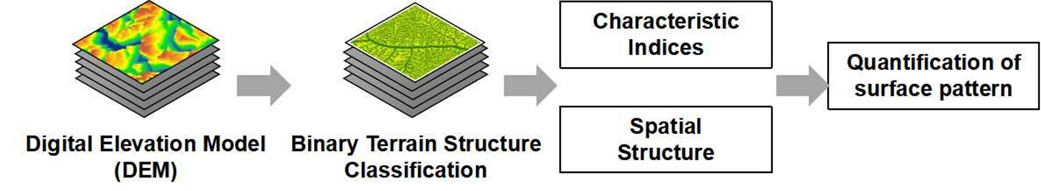
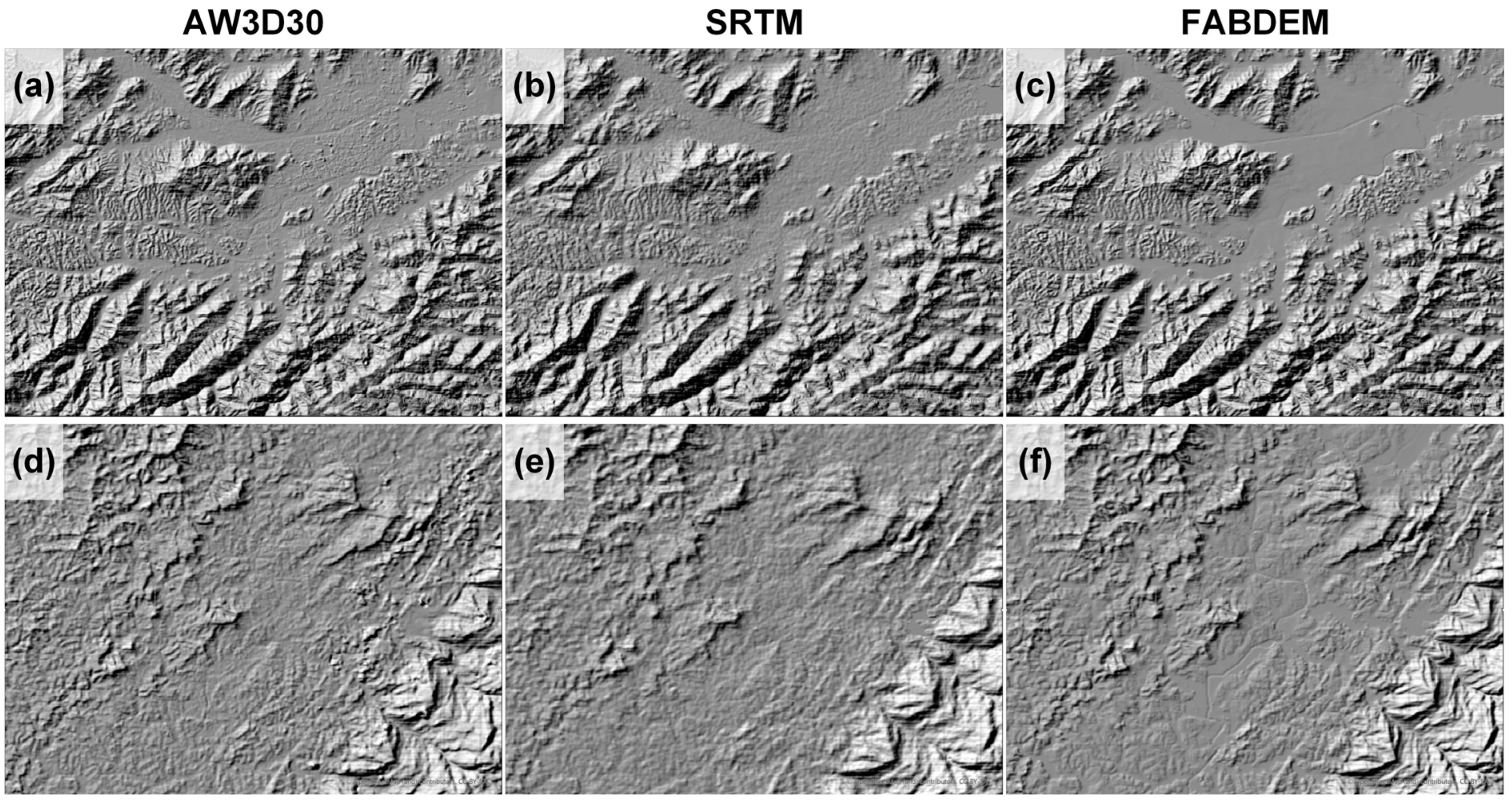
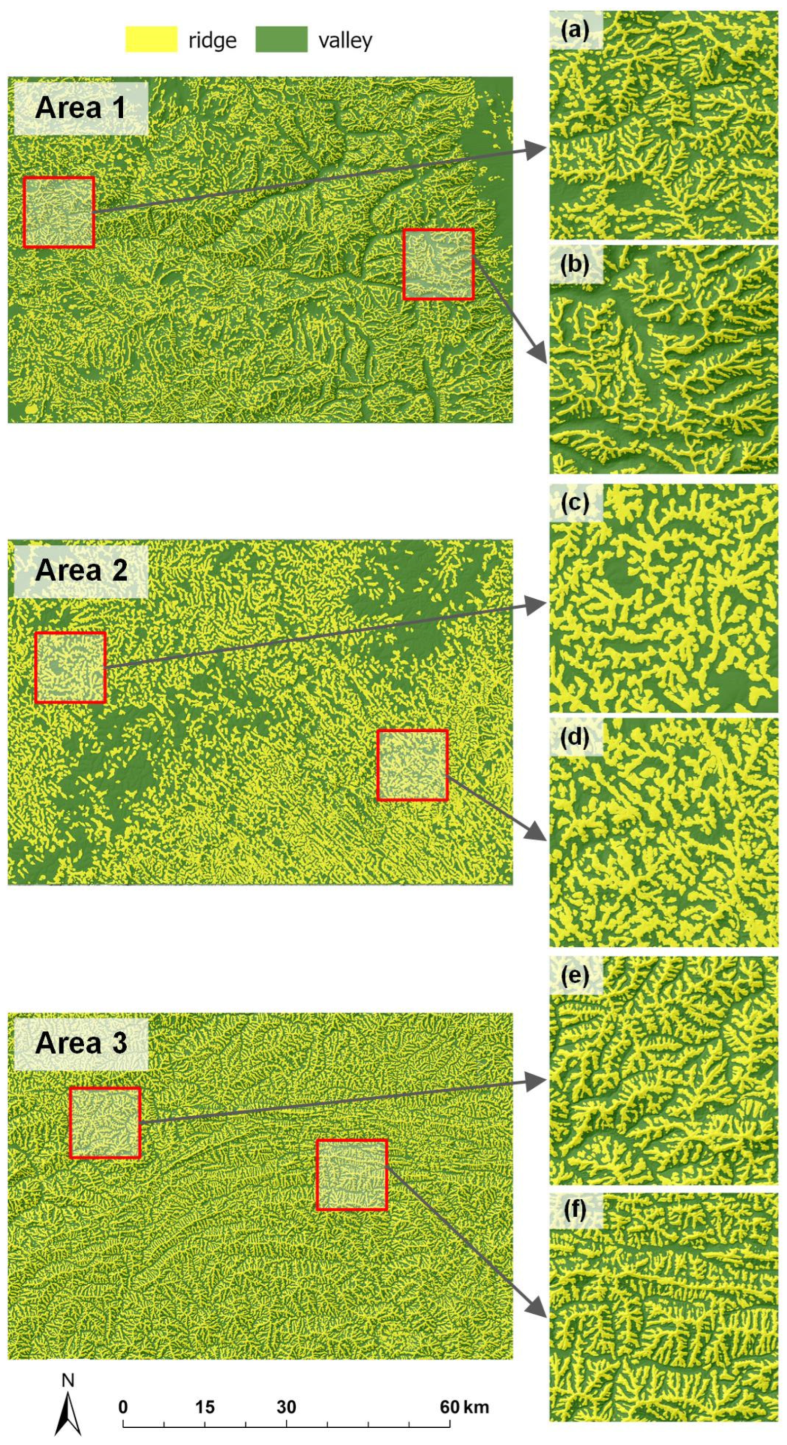
2.1. Data and Study Areas
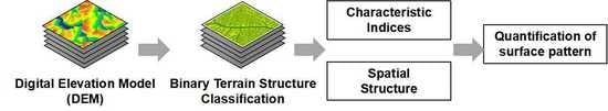
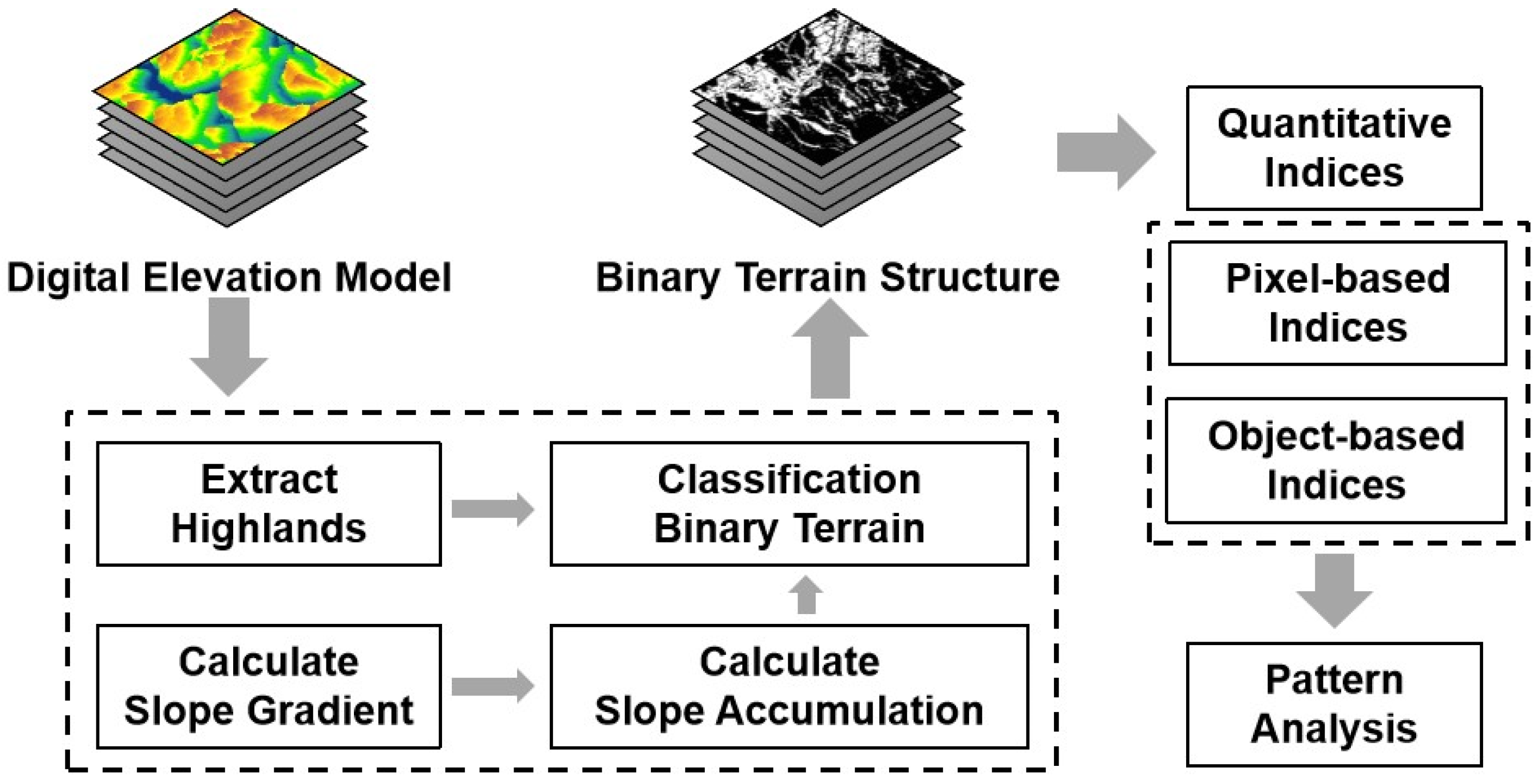
In this paper, we regard the Forest And Buildings removed Copernicus Digital Elevation Model (FABDEM) [50] as the basic data to classify the binary terrain. FABDEM is the acronym for forest and buildings removed Copernicus DEM. Researchers used machine learning to remove buildings and forests from the Copernicus Digital Elevation Model to produce this dataset [50]. FABDEM has a spatial resolution of one arc-second (approximately 30 m). As shown in Figure 1, FABDEM reduces the roughness caused by buildings and canopies, especially in mountainous areas with forests. The aim of our study is to classify the binary terrain with natural attributes, while complex land cover can negatively influence the classification of binary terrain. Thus, the removal of forests and buildings achieved by FABDEM is beneficial for our study to optimize the classification of surface objects. In addition, the comparison of FABDEM, LiDAR data, Copernicus DEM, ICESat-2 and other DEMs demonstrates the utility of the FABDEM dataset [50,60,61]. In addition, to assess the transferability of the proposed method across different DEMs, we introduce Shuttle Radar Topography Mission (SRTM) [62] and ALOS World 3D–30 m (AW3D30) [63] DEMs as additional datasets. These two DEMs contain land cover information and are obtained from Google Earth Engine. As shown in Figure 1, FABDEM reduces the influence of forests and buildings on the surface texture. It has been suggested that FABDEM can support various geographic studies, including flood analysis [64,65] and object extraction [66].
We collected DEMs in three study areas of South America (Area 1), North America (Area 2) and Asia (Area 3) (Figure 2). Area 1 (Figure 2b) and Area 3 (Figure 2d) are in the Rocky Mountains and the Loess Plateau, respectively, and contain typical mountains and plains. Area 2 (Figure 2c) is in a region with hills and gentle slopes. The experiments completed in these three areas can indicate the robustness of the proposed method.

2.2. Methods

In this paper, we focus on the binary terrain that can reflect the surface structure at a regional scale in mountainous areas. As shown in Figure 3, the method proposed in this paper consists of three steps: (1) extraction of local highlands that represent the peaks or ridges with convex shapes; (2) calculation of the slope gradient and SA to reflect topographic characteristics; and (3) segmentation of the binary terrain based on adaptive thresholds.

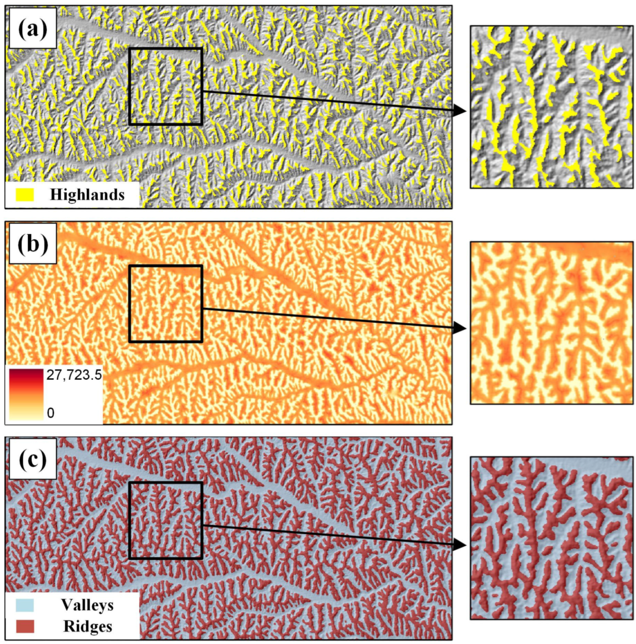
2.2.1. Extraction of Highlands

In mountainous areas, ridges could be regarded as the extension of highlands that have relatively high elevations. In this step, we focus on the extraction of highlands. Initially, we calculate the difference between the original elevation and the mean elevation based on the analysis window with a size of 17 × 17 pixels [67]. Then, a threshold of 20 m is applied to extract the local highlands. The highlands (Figure 4a) have elevation differences that are greater than 20 m and represent a part of peaks or ridges in mountainous areas. According to previous studies [23,68], mountains are usually defined as objects with terrain relief greater than 30 m. In these studies, the terrain relief represents the elevation difference between the highest pixel and the lowest pixel in an analysis window. It is difficult to define a stable threshold based on the above terrain relief to extract ridge areas, especially in mountainous areas, due to the severe terrain relief and large elevation range. Therefore, we calculate the difference between the original elevation and the mean elevation to reflect the relative relief in the analysis window. Integrating this information with expert knowledge, we reduce the previous threshold to 20 m to extract areas with relatively large elevations. These highlands will be utilized in the next step as the basic data to classify the binary terrain.

2.2.2. Calculation of Slope Accumulation

In this paper, we propose a new terrain derivative referred to as SA that represents the long distance relationship of the slope gradient between two different locations. This method uses the local highlands as the target area and the slope gradient as the cost raster to identify the path with the least cost to reach the highlands at each location. Then, we calculate the sum of the slope gradient along the path with the least cost and regard the sum slope as the SA.
In detail, first, the slope is calculated based on DEMs. This process computes the rate of surface change in the horizontal and vertical directions from the centre cell to each adjacent cell. Second, we calculate the SA for each cell according to the principle of distance accumulation [69]. In this process, the local highlands extracted in Section 2.2.1 and the slope gradient are regarded as the source and cost raster, respectively. Then, this algorithm will reveal the path with the least accumulated cost from each cell to the sources. The results of SA are shown in Figure 4b.

2.2.3. Segmentation of the Binary Terrain

After the calculation of SA, it is necessary to determine suitable rules to segment the binary terrains. In this step, we design an adaptive threshold that can automatically adjust with the changing of study areas. Two issues need to be considered in the determination of the SA threshold for landform classification. First, due to the accumulated attributes of SA, the boundary constructed by segmenting the SA raster indicates the potential location of the qualitative change in terrain. The completeness and geomorphological semantics of segmented objects should be considered in the determination of thresholds. Second, the various geographic scenarios increase the suitable classification of binary terrains in different areas. The designed threshold should be tested in areas with different landforms. Based on the consideration of these two issues, we constructed an adaptive SA threshold to achieve binary terrain classification. The adaptive threshold of SA is calculated as follows:
T S A = S A l q / 2 ,
where T S A is the SA adaptive threshold, and S A l q is the lower quartile of SA. The segmented results are shown in Figure 4c.

2.3. Indices

The selection of quantitative derivatives is significant for the comprehensive analysis of surface patterns. The above steps achieve the classification of binary terrain and provided objects with different topographic categories. In this step, considering the multidimensional characteristics of topographic patterns, we select several quantitative indices from the perspective of cell- and object-based analysis.

2.3.1. Pixel-Based Indices

Pixel-based analysis considers the quantitative characteristics of each cell and calculates derivatives to reflect the category, topography and other features. In this section, we select plan curvature, profile curvature and class ratio as the cell-based derivatives to quantitatively evaluate surface patterns.
Curvature is one of the most significant derivatives to describe the shape of a surface. It is helpful to quantify the terrain changes in landform development. Curvature can be further classified according to the different calculating directions. Profile and plan curvatures are two common curvatures with complementary analysis perspectives. Profile curvature represents the geometric normal curvature along the slope line, while plan curvature is the curvature along the contour lines. The positive values and negative values of profile and plan curvatures indicate the shape of the surface (e.g., concave and convex shapes) at that cell in directions along the slope lines and contour lines, respectively. These curvatures quantitatively reflect the shape of the topographic objects and help compare the ridges and valleys. The formulas for calculating the profile and plan curvatures are presented as follows [70,71]:
C p r o = f x x f x 2 2 f x y f x f y + f y y f y 2 f x 2 + f y 2 1 + f x 2 + f y 2 3 / 2 ,
C p l a = f x x f y 2 2 f x y f x f y + f y y f x 2 f x 2 + f y 2 3 / 2 ,
where C p r o and C p l a represent profile and plan curvatures, respectively.
The class ratio reflects the element composition of topographic structure in a specific area. A similar index has been used to analyze the P-N terrain [23]. The ratio of different topographic objects is usually related to the development stage of landforms. Several studies have discussed this connection. In this paper, we compute the class ratio [19] as follows:
C R = C r C v ,
where C R represents the class ratio, and C r and C v represent the pixel counts of ridges and valleys, respectively.

2.3.2. Object-Based Indices

In this paper, due to the construction of the binary terrain structure, we can achieve further analysis from an object-based perspective. The classification of the binary terrain constructs topographic objects with different classes. The shape and distribution of these objects are also helpful for revealing surface patterns in areas with different landforms. Therefore, we employ three object-based indices (as shown in Table 1) as complements to show the surface patterns.

3. Results

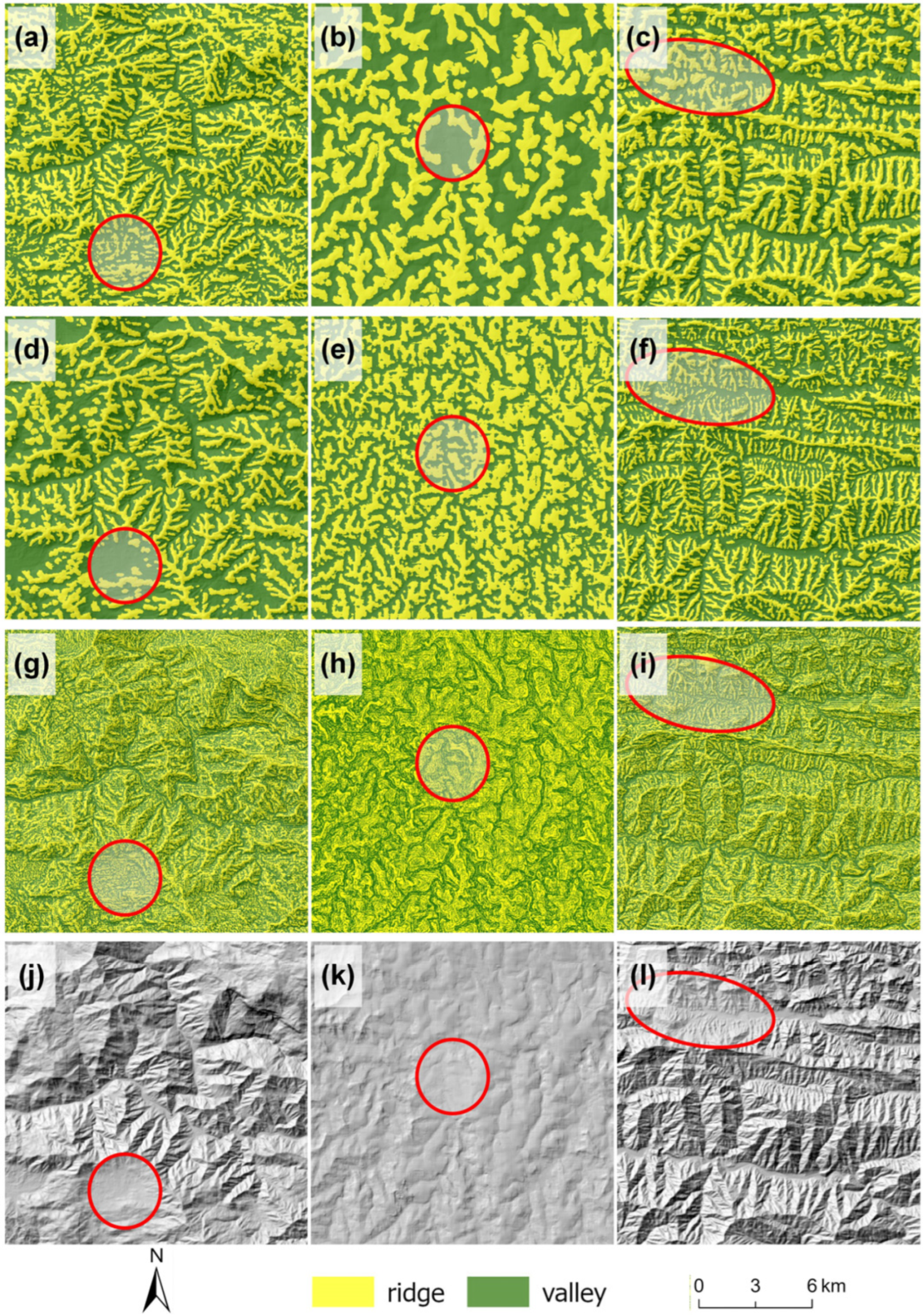
3.1. Classification of the Binary Terrain

Figure 5 displays the classification of the binary terrain in the three study areas. In general, the segmented results reflect the basic surface structure consisting of ridges and valleys. As we mentioned in Section 2.3, Areas 1 and 3 are mountainous areas and contain typical ridges and valleys. The results in Figure 5a,c reflect these findings qualitatively and digitally and support the quantitative analysis. In detail, the ridge blocks in Area 1 are thinner than those in Area 3. This phenomenon indicates that the surface of Area 1 is steeper than that of Area 3, which leads to a high SA value over a relatively short distance. Therefore, the binary terrain segmented by our method can reflect the differences in detailed topographic structure even in areas with similar landforms. Figure 5b illustrates the topographic structure in hills, which is different from the other two study areas. The ridges in Area 2 have a smoother boundary than those in Areas 1 and 3. Plains in valleys with large areas can also be observed in the northeastern and southwestern regions of Area 2. In addition, the ridge blocks in Figure 5b generally have a larger width than those in Areas 1 and 3. This phenomenon relates to the gentle slope gradient in Area 2 with numerous hills.

3.2. Method Comparison

To evaluate the performance of the proposed method, we completed comparison experiments with the method based on the elevation difference and based on the profile curvature difference. Figure 6 shows detailed differences among these methods. Two phenomena were observed via the results comparison. First, our method efficiently improves ridge classification, especially in flat areas. Many broken ridge blocks are observed in Figure 6d,g and denoted by red circles. These broken blocks could be caused by the local terrain relief, which significantly influences the window-based calculation. In addition, as shown in the second column of Figure 6, our results avoid the oversimplification shown in Figure 6e and incorrect expression shown in Figure 6h. This phenomenon also suggests the better performance of our method compared to the other two methods. Second, the proposed method can extract more complete mountain areas than the previous method. Figure 6c,f,i show the results in Area 3, which has a high density of ridges. The intense relief and frequent changes in different topographic objects increase the difficulty of segmenting the binary terrain. The results of the previous methods (Figure 6f,i) show the basic surface structure with a mountainous texture. However, the ridge blocks in Figure 6f,i have small areas and pseudoridges that reduce the availability of these results. The thin ridge blocks with complicated boundaries cannot display the complete ridge areas and lead to deviation in assessing the class ratio of the topographic structure. As shown in Figure 6c, our method provides a clearer structure of the surface and reduces the pseudoblocks, as we previously analyzed. This new method also reduces the number of scattered blocks with small areas, which could reduce the analysis efficiency.
In summary, the classification method proposed in this paper outperforms the previous methods and can efficiently support the understanding of surface patterns. The segmented results achieve satisfactory performances in different scenarios, including valleys with flat areas and typical mountainous areas.

3.3. Calculated Quantitative Indices

Table 2 shows the mean profile curvature, mean plan curvature and class ratio in three areas based on the segmented binary terrains. It is distinct that ridges and valleys segmented by the proposed method display a large difference in the value of curvatures. Ridges in all study areas have positive curvature values, while valleys show negative curvatures. The curvature results reflect the shape differences of ridges and valleys and suggest the availability of the proposed method to segment binary terrain. In addition, the morphological differences between ridges and valleys can be obtained through the results comparison for the three areas. Ridges in Areas 1 and 3 have similar profile curvatures but different plan curvatures. This finding shows that the ridges in Area 1 have a similar shape in the direction along the slope line but a smoother boundary in the direction along the contour line than that in Area 3. The valleys in Area 3 show totally different topographic characteristics indicated by the profile and plan curvatures with great differences. The ridges in Area 2 contain the smallest plan curvature and largest profile curvature. This phenomenon is possibly attributed to the numerous isolated mountains in Area 2.
Figure 7 displays the results of the PARA and FDI in the study areas. First, the results of these two indices reflect the obvious shape differences of ridges and valleys. The PARA and FDI values of ridges and valleys are distributed into different ranges, which further suggests the validity of the proposed method to segment the binary terrain structure. In all three areas, the PARA values of valleys are larger than those of ridges, but the FDI values are smaller than those of ridges. As PARA is sensitive to the size of blocks, this phenomenon can reflect that ridge blocks segmented by the proposed method have more complex shapes but smaller areas than valley blocks. In detail, a similar phenomenon was observed in specific areas. For ridges, Areas 1, 2 and 3 have similar FDIs, but Area 2 has a relatively small PARA. Considering the meaning of PARA and FDI, this phenomenon indicates that ridge blocks in Area 2 are smaller than those in other areas and further supports the abovementioned conclusion that Area 2 contains many isolated mountains with a small area. In addition, valleys in Areas 1 and 2 show similar FDIs but different PARAs, which suggests that Area 1 has larger and more complete valleys than Area 2.
We show the LSI values and their spatial distribution in Figure 8. Generally, the three study areas display different LSI distributions. Area 3 (Figure 8c) has numerous cells with a large LSI, especially in the direction of southwest to northeast, which has a concentrated distribution of large LSI values. This finding suggests that the surface pattern in Area 3 is more complex than that in other areas from the perspective of landscape complexity. Due to the influence of plains in valleys, Figure 8b, which represents the LSI of Area 2, displays two obvious regions with small LSI values, and a similar region is observed in the northeastern corner of Figure 8a. This finding indicates that the LSI calculated based on the segmented binary terrain can display the spatial distribution of valleys and ridges. Therefore, based on the above analysis, we can quantitatively analyze the surface pattern based on the segmented binary terrain, which considers the morphological characteristics and spatial distribution of topographic objects.

4. Discussion

4.1. Transferability of the Proposed Method

To evaluate the transferability of the proposed method, we completed the terrain classification based on different DEMs in the test areas. Figure 8 shows the classification results based on different DEMs, including FABDEM, AW3D30 and SRTM data. The results show that the proposed method achieves similar results across different data conditions. In detail, a slight loss of ridges is observed in Figure 9, especially in a subregion of Area 3 (Figure 9c,f,i). In Figure 9b,e,h, the use of different DEMs yields slight morphological differences in ridges in the middle of the experimental area. These differences are mainly dominated by the quality of data sources. This phenomenon has a limited effect on the distribution of ridges and valleys in the classification results. Thus, this experiment suggests that this new method is transferable to different DEMs.

4.2. Quantitative Analysis of the Surface Pattern

The comprehensive evaluation of the surface pattern benefits further understanding of the spatial difference of the Earth’s surface. Considering the various content in the surface pattern, we selected several pixel-based and object-based indices to quantitatively evaluate the surface based on the segmented results and then analyze the surface patterns. First, the profile and plan curvatures are common derivatives that reflect the topographic characteristics. The curvature results show great differences between ridges and valleys and vary in three areas on different continents. The class ratio displays the composition of topographic objects from the perspective of the binary terrain structure. The PARA and FDI evaluate the shape complexity of landform objects with quantitative results, and the LSI provides information about the spatial distribution of landforms. The combination of these indices calculated based on the binary terrain structure provides a chance to understand the surface patterns from a quantitative perspective.
The results of the quantitative indices indicate the differences among areas in different locations. Generally, the three study areas in this paper show different surface patterns. Area 1 in the Rocky Mountains contains wide and steep valleys indicated by the small class ratio, large absolute profile curvature and a large PARA. Area 2 in North America has concentrated plains in valleys with large areas and relatively simple ridge boundaries. Numerous isolated ridges in Area 2 are also reflected by the quantitative indices. Area 3 has the most complex terrain structure, reflected by a high LSI. Considering the high class ratio and LSI, it is suggested that Area 3 includes a more frequent transition of ridges and valleys than the other two areas.

4.3. Limitations and Next Steps

Although the proposed method achieves good results in the classification of binary terrain, further improvements could be completed in future work. In this paper, we consider the ridge and valley as elements of binary terrain. The terms of these basic elements could be updated in areas with different landforms to support research in wider regions. For example, in an area with the loess landform, the binary terrain consists of the loess ridge and loess gully [20], while Fenglin and Fengcon [74] compose the binary terrain of the karst landform. The proposed method provides a general idea to construct the binary structure of the Earth’s surface, but in a specific area, it is necessary to adjust the terms of the binary terrain. In addition, it is valuable to generate more classes with detailed attribute differences based on the binary structure. The binary terrain constructed in this paper can be further segmented into blocks with low-level classes according to multiple factors. The construction of a hierarchical object system would benefit geomorphological research at various scales. In this process, the integration of data with various types and resolutions could be discussed to solve the potential issues in the classification. The topographic fusion is helpful for more accurate classification and deeper understanding than before. Furthermore, we still need to consider the integration of the current method and orogenic processes that significantly influence surface morphology. The connection between these two factors can help us understand the relationship between the surface structure and Earth formation.

5. Conclusions

In this paper, we propose a new method to classify the binary terrain structure and verify its availability in areas with different landforms. This new method emphasizes the accumulated characteristics of terrain relief and provides a new topographic derivative referred to as SA. The proposed method includes four steps: the extraction of highlands, calculation of the slope gradient, calculation of SA and segmentation of the binary terrain. We optimized the method by considering local and accumulated surface characteristics to reduce the uncertainty in the classification and increase the completeness of the segmented results. The results show that our method outperforms previous studies in different areas and can provide a binary terrain structure with fewer broken blocks. The experiments in areas with different landforms suggest the transferability of the proposed method in various areas. The segmented objects can be regarded as the analysis units for geographic research and benefit land management and slope mapping.
This paper provides a practical way to quantitatively describe surface patterns. We constructed a combination of various indices to comprehensively express terrain characteristics. In detail, we considered the topographic characteristics, category composition, object morphology and landform spatial distribution in the selection of quantitative indices. Compared to previous studies, the results in this paper express not only the differences in objects in the binary terrain structure but also the various patterns in three areas on different continents.

Author Contributions

Conceptualization, S.L. and X.Y.; methodology, S.L. and X.Y.; software, S.L. and X.Z.; validation, S.L. and X.Z.; resources, X.Z.; writing—original draft preparation, S.L.; writing—review and editing, S.L. and G.T.; visualization, S.L.; supervision, X.Y. and G.T.; funding acquisition, X.Y. and G.T. All authors have read and agreed to the published version of the manuscript.

Funding

This research was supported by the National Natural Science Foundation of China (grant numbers: 42171402; 41930102), the Priority Academic Program Development of Jiangsu Higher Education Institutions and the Deep-time Digital Earth (DDE) Big Science Program.

Data Availability Statement

The data presented in this study are available on reasonable request from the corresponding author.

Acknowledgments

The authors express their gratitude towards the editors.

Conflicts of Interest

The authors declare no conflict of interest.

References

  1. Evans, I.S. Geomorphometry and landform mapping: What is a landform? Geomorphology 2012, 137, 94–106. [Google Scholar] [CrossRef]
  2. Xiong, L.; Li, S.; Tang, G.; Strobl, J. Geomorphometry and terrain analysis: Data, methods, platforms and applications. Earth-Sci. Rev. 2022, 233, 104191. [Google Scholar] [CrossRef]
  3. Fu, B. Soil erosion and its control in the Loess Plateau of China. Soil Use Manag. 1989, 5, 76–82. [Google Scholar] [CrossRef]
  4. Hengl, T.; Reuter, H.I. Geomorphometry: Concepts, Software, Applications; Newnes: Oxford, UK, 2008. [Google Scholar]
  5. Florinsky, I.V. An illustrated introduction to general geomorphometry. Prog. Phys. Geogr. 2017, 41, 723–752. [Google Scholar] [CrossRef]
  6. Wilson, J.P. Geomorphometry: Today and tomorrow. PeerJ Prepr. 2018, 6, e27197v1. [Google Scholar]
  7. Wilson, J.P.; Gallant, J.C. Terrain Analysis: Principles and Applications; John Wiley & Sons: Hoboken, NJ, USA, 2000. [Google Scholar]
  8. Fressard, M.; Cossart, E. A graph theory tool for assessing structural sediment connectivity: Development and application in the Mercurey vineyards (France). Sci. Total Environ. 2019, 651, 2566–2584. [Google Scholar] [CrossRef]
  9. Minár, J.; Evans, I.S.; Jenčo, M. A comprehensive system of definitions of land surface (topographic) curvatures, with implications for their application in geoscience modelling and prediction. Earth-Sci. Rev. 2020, 211, 103414. [Google Scholar] [CrossRef]
  10. Zhilin, L. Multi-scale digital terrain modelling and analysis. In Advances in Digital Terrain Analysis; Springer: Berlin/Heidelberg, Germany, 2008; pp. 59–83. [Google Scholar]
  11. Maxwell, A.E.; Shobe, C.M. Land-surface parameters for spatial predictive mapping and modeling. Earth-Sci. Rev. 2022, 226, 103944. [Google Scholar] [CrossRef]
  12. Pike, R.J. Geomorphometry-diversity in quantitative surface analysis. Prog. Phys. Geogr. 2000, 24, 1–20. [Google Scholar]
  13. Elsen, P.R.; Monahan, W.B.; Merenlender, A.M. Global patterns of protection of elevational gradients in mountain ranges. Proc. Natl. Acad. Sci. USA 2018, 115, 6004–6009. [Google Scholar] [CrossRef]
  14. Ochtyra, A. Forest disturbances in polish Tatra mountains for 1985–2016 in relation to topography, stand features, and protection zone. Forests 2020, 11, 579. [Google Scholar] [CrossRef]
  15. Fu, B.J.; Zhao, W.W.; Chen, L.D.; Zhang, Q.J.; Lü, Y.; Gulinck, H.; Poesen, J. Assessment of soil erosion at large watershed scale using RUSLE and GIS: A case study in the Loess Plateau of China. Land Degrad. Dev. 2005, 16, 73–85. [Google Scholar] [CrossRef]
  16. Nguyen, K.A.; Chen, W. DEM-and GIS-Based Analysis of Soil Erosion Depth Using Machine Learning. ISPRS Int. J. Geo-Inf. 2021, 10, 452. [Google Scholar] [CrossRef]
  17. Maeda, E.E.; Clark, B.J.; Pellikka, P.; Siljander, M. Modelling agricultural expansion in Kenya’s Eastern Arc Mountains biodiversity hotspot. Agric. Syst. 2010, 103, 609–620. [Google Scholar] [CrossRef]
  18. Muellner-Riehl, A.N.; Schnitzler, J.; Kissling, W.D.; Mosbrugger, V.; Rijsdijk, K.F.; Seijmonsbergen, A.C.; Versteegh, H.; Favre, A. Origins of global mountain plant biodiversity: Testing the ‘mountain-geobiodiversity hypothesis’. J. Biogeogr. 2019, 46, 2826–2838. [Google Scholar] [CrossRef]
  19. Li, S.; Xiong, L.; Tang, G.; Strobl, J. Deep learning-based approach for landform classification from integrated data sources of digital elevation model and imagery. Geomorphology 2020, 354, 107045. [Google Scholar] [CrossRef]
  20. Liu, K.; Ding, H.; Tang, G.; Na, J.; Huang, X.; Xue, Z.; Yang, X.; Li, F. Detection of catchment-scale gully-affected areas using unmanned aerial vehicle (UAV) on the Chinese Loess Plateau. ISPRS Int. J. Geo-Inf. 2016, 5, 238. [Google Scholar] [CrossRef]
  21. Drăguţ, L.; Eisank, C. Automated object-based classification of topography from SRTM data. Geomorphology 2012, 141, 21–33. [Google Scholar] [CrossRef]
  22. Ding, H.; Liu, K.; Chen, X.; Xiong, L.; Tang, G.; Qiu, F.; Strobl, J. Optimized segmentation based on the weighted aggregation method for loess bank gully mapping. Remote Sens. 2020, 12, 793. [Google Scholar] [CrossRef]
  23. Zhou, Y.; Tang, G.A.; Yang, X.; Xiao, C.; Zhang, Y.; Luo, M. Positive and negative terrains on northern Shaanxi Loess Plateau. J. Geogr. Sci. 2010, 20, 64–76. [Google Scholar] [CrossRef]
  24. Cavalli, M.; Goldin, B.; Comiti, F.; Brardinoni, F.; Marchi, L. Assessment of erosion and deposition in steep mountain basins by differencing sequential digital terrain models. Geomorphology 2017, 291, 4–16. [Google Scholar] [CrossRef]
  25. Hu, G.; Dai, W.; Li, S.; Xiong, L.; Tang, G.; Strobl, J. Quantification of terrain plan concavity and convexity using aspect vectors from digital elevation models. Geomorphology 2021, 375, 107553. [Google Scholar] [CrossRef]
  26. Jasiewicz, J.; Stepinski, T.F. Geomorphons—A pattern recognition approach to classification and mapping of landforms. Geomorphology 2013, 182, 147–156. [Google Scholar] [CrossRef]
  27. Hu, G.; Xiong, L.; Lu, S.; Chen, J.; Li, S.; Tang, G.; Strobl, J. Mathematical vector framework for gravity-specific land surface curvatures calculation from triangulated irregular networks. GIScience Remote Sens. 2022, 59, 590–608. [Google Scholar] [CrossRef]
  28. Libohova, Z.; Winzeler, H.E.; Lee, B.; Schoeneberger, P.J.; Datta, J.; Owens, P.R. Geomorphons: Landform and property predictions in a glacial moraine in Indiana landscapes. CATENA 2016, 142, 66–76. [Google Scholar] [CrossRef]
  29. Xiong, L.; Tang, G.; Yan, S.; Zhu, S.; Sun, Y. Landform-oriented flow-routing algorithm for the dual-structure loess terrain based on digital elevation models. Hydrol. Process. 2014, 28, 1756–1766. [Google Scholar] [CrossRef]
  30. Yang, F.; Zhou, Y. Quantifying spatial scale of positive and negative terrains pattern at watershed-scale: Case in soil and water conservation region on Loess Plateau. J. Mt. Sci. 2017, 14, 1642–1654. [Google Scholar] [CrossRef]
  31. Lin, S.; Chen, N.; He, Z. Automatic landform recognition from the perspective of watershed spatial structure based on digital elevation models. Remote Sens. 2021, 13, 3926. [Google Scholar] [CrossRef]
  32. Tang, G.; Li, F.; Xiong, L. Progress of Digital Terrain Analysis in the Loess Plateau of China. Geogr. Geo-Inf. Sci. 2017, 33, 1–7. [Google Scholar]
  33. Tarolli, P.; Sofia, G.; Dalla Fontana, G. Geomorphic features extraction from high-resolution topography: Landslide crowns and bank erosion. Nat. Hazards 2012, 61, 65–83. [Google Scholar] [CrossRef]
  34. Prosdocimi, M.; Calligaro, S.; Sofia, G.; Dalla Fontana, G.; Tarolli, P. Bank erosion in agricultural drainage networks: New challenges from structure-from-motion photogrammetry for post-event analysis. Earth Surf. Process. Landf. 2015, 40, 1891–1906. [Google Scholar] [CrossRef]
  35. Sofia, G. Combining geomorphometry, feature extraction techniques and Earth-surface processes research: The way forward. Geomorphology 2020, 355, 107055. [Google Scholar] [CrossRef]
  36. Li, W.; Hsu, C.-Y. Automated terrain feature identification from remote sensing imagery: A deep learning approach. Int. J. Geogr. Inf. Sci. 2020, 34, 637–660. [Google Scholar] [CrossRef]
  37. Li, W.; Zhou, B.; Hsu, C.-Y.; Li, Y.; Ren, F. Recognizing terrain features on terrestrial surface using a deep learning model: An example with crater detection. In Proceedings of the 1st Workshop on Artificial Intelligence and Deep Learning for Geographic Knowledge Discovery, Los Angeles, CA, USA, 7–10 November 2017; pp. 33–36. [Google Scholar]
  38. Huang, L.; Liu, L.; Jiang, L.; Zhang, T. Automatic mapping of thermokarst landforms from remote sensing images using deep learning: A case study in the Northeastern Tibetan Plateau. Remote Sens. 2018, 10, 2067. [Google Scholar] [CrossRef]
  39. Zhao, W.; Persello, C.; Stein, A. Extracting planar roof structures from very high resolution images using graph neural networks. ISPRS J. Photogramm. Remote Sens. 2022, 187, 34–45. [Google Scholar] [CrossRef]
  40. Li, S.; Hu, G.; Cheng, X.; Xiong, L.; Tang, G.; Strobl, J. Integrating topographic knowledge into deep learning for the void-filling of digital elevation models. Remote Sens. Environ. 2022, 269, 112818. [Google Scholar] [CrossRef]
  41. Gioia, D.; Danese, M.; Corrado, G.; Di Leo, P.; Minervino Amodio, A.; Schiattarella, M. Assessing the prediction accuracy of geomorphon-based automated landform classification: An example from the ionian coastal belt of southern Italy. ISPRS Int. J. Geo-Inf. 2021, 10, 725. [Google Scholar] [CrossRef]
  42. Diani, K.; Tabyaoui, H.; Kacimi, I.; El Hammichi, F.; Nakhcha, C. Stream Network Modelling from Aster GDEM Using ArcHydro GIS: Application to the Upper Moulouya River Basin (Eastern, Morocco). J. Geosci. Environ. Prot. 2017, 5, 1. [Google Scholar] [CrossRef]
  43. Dai, W.; Hu, G.-H.; Yang, X.; Yang, X.-W.; Cheng, Y.-H.; Xiong, L.-Y.; Strobl, J.; Tang, G.-A. Identifying ephemeral gullies from high-resolution images and DEMs using flow-directional detection. J. Mt. Sci. 2020, 17, 3024–3038. [Google Scholar] [CrossRef]
  44. Wilson, J.P. Digital terrain modeling. Geomorphology 2012, 137, 107–121. [Google Scholar] [CrossRef]
  45. Irvin, B.J.; Ventura, S.J.; Slater, B.K. Fuzzy and isodata classification of landform elements from digital terrain data in Pleasant Valley, Wisconsin. Geoderma 1997, 77, 137–154. [Google Scholar] [CrossRef]
  46. Liu, K.; Ding, H.; Tang, G.; Song, C.; Liu, Y.; Jiang, L.; Zhao, B.; Gao, Y.; Ma, R. Large-scale mapping of gully-affected areas: An approach integrating Google Earth images and terrain skeleton information. Geomorphology 2018, 314, 13–26. [Google Scholar] [CrossRef]
  47. Minar, J.; Evans, I.S. Elementary forms for land surface segmentation: The theoretical basis of terrain analysis and geomorphological mapping. Geomorphology 2008, 95, 236–259. [Google Scholar] [CrossRef]
  48. Iwahashi, J.; Kamiya, I.; Matsuoka, M.; Yamazaki, D. Global terrain classification using 280 m DEMs: Segmentation, clustering, and reclassification. Prog. Earth Planet. Sci. 2018, 5, 1. [Google Scholar] [CrossRef]
  49. Drăguţ, L.; Blaschke, T. Automated classification of landform elements using object-based image analysis. Geomorphology 2006, 81, 330–344. [Google Scholar] [CrossRef]
  50. Hawker, L.; Uhe, P.; Paulo, L.; Sosa, J.; Savage, J.; Sampson, C.; Neal, J. A 30 m global map of elevation with forests and buildings removed. Environ. Res. Lett. 2022, 17, 024016. [Google Scholar] [CrossRef]
  51. Hutchinson, M. ANUDEM Version 5.3, User Guide; Fenner School of Environment and Society, Australian National University: Canberra, Australia, 2011. [Google Scholar]
  52. Na, J.; Ding, H.; Zhao, W.; Liu, K.; Tang, G.; Pfeifer, N. Object-based large-scale terrain classification combined with segmentation optimization and terrain features: A case study in China. Trans. GIS 2021, 25, 2939–2962. [Google Scholar] [CrossRef]
  53. Na, J.; Yang, X.; Tang, G.; Dang, W.; Strobl, J. Population characteristics of loess gully system in the Loess Plateau of China. Remote Sens. 2020, 12, 2639. [Google Scholar] [CrossRef]
  54. Xiong, L.; Tang, G.; Yang, X.; Li, F. Geomorphology-oriented digital terrain analysis: Progress and perspectives. J. Geogr. Sci. 2021, 31, 456–476. [Google Scholar] [CrossRef]
  55. Webster, T.L.; Dias, G. An automated GIS procedure for comparing GPS and proximal LiDAR elevations. Comput. Geosci. 2006, 32, 713–726. [Google Scholar] [CrossRef]
  56. Muthusamy, M.; Casado, M.R.; Butler, D.; Leinster, P. Understanding the effects of Digital Elevation Model resolution in urban fluvial flood modelling. J. Hydrol. 2021, 596, 126088. [Google Scholar] [CrossRef]
  57. Liu, K.; Song, C.; Ke, L.; Jiang, L.; Ma, R. Automatic watershed delineation in the Tibetan endorheic basin: A lake-oriented approach based on digital elevation models. Geomorphology 2020, 358, 107127. [Google Scholar] [CrossRef]
  58. Xu, Y.; Zhang, S.; Li, J.; Liu, H.; Zhu, H. Extracting Terrain Texture Features for Landform Classification Using Wavelet Decomposition. ISPRS Int. J. Geo-Inf. 2021, 10, 658. [Google Scholar] [CrossRef]
  59. Ding, H.; Na, J.-m.; Huang, X.-l.; Tang, G.-a.; Liu, K. Stability analysis unit and spatial distribution pattern of the terrain texture in the northern Shaanxi Loess Plateau. J. Mt. Sci. 2018, 15, 577–589. [Google Scholar] [CrossRef]
  60. Dandabathula, G.; Hari, R.; Ghosh, K.; Bera, A.K.; Srivastav, S.K. Accuracy assessment of digital bare-earth model using ICESat-2 photons: Analysis of the FABDEM. In Modeling Earth Systems and Environment; Springer: Cham, Switzerland, 2022. [Google Scholar]
  61. Marsh, C.B.; Harder, P.; Pomeroy, J.W. Validation of FABDEM, a global bare-earth elevation model, against UAV-lidar derived elevation in a complex forested mountain catchment. Environ. Res. Commun. 2023, 5, 031009. [Google Scholar] [CrossRef]
  62. Farr, T.G.; Rosen, P.A.; Caro, E.; Crippen, R.; Duren, R.; Hensley, S.; Kobrick, M.; Paller, M.; Rodriguez, E.; Roth, L. The shuttle radar topography mission. Rev. Geophys. 2007, 45, 2. [Google Scholar] [CrossRef]
  63. Takaku, J.; Tadono, T.; Tsutsui, K. Generation of High Resolution Global DSM from ALOS PRISM. ISPRS Arch. 2014, XL-4, 243–248. [Google Scholar] [CrossRef]
  64. Teng, J.; Penton, D.; Ticehurst, C.; Sengupta, A.; Freebairn, A.; Marvanek, S.; Vaze, J.; Gibbs, M.; Streeton, N.; Karim, F. A Comprehensive Assessment of Floodwater Depth Estimation Models in Semiarid Regions. Water Resour. Res. 2022, 58, e2022WR032031. [Google Scholar] [CrossRef]
  65. Vernimmen, R.; Hooijer, A. New LiDAR-Based Elevation Model Shows Greatest Increase in Global Coastal Exposure to Flooding to Be Caused by Early-Stage Sea-Level Rise. Earth’s Future 2023, 11, e2022EF002880. [Google Scholar] [CrossRef]
  66. Chen, Y.; Yang, X.; Yang, L.; Feng, J. An Automatic Approach to Extracting Large-Scale Three-Dimensional Road Networks Using Open-Source Data. Remote Sens. 2022, 14, 5746. [Google Scholar] [CrossRef]
  67. Li, S.; Xiong, L.; Hu, G.; Dang, W.; Tang, G.; Strobl, J. Extracting check dam areas from high-resolution imagery based on the integration of object-based image analysis and deep learning. Land Degrad. Dev. 2021, 32, 2303–2317. [Google Scholar] [CrossRef]
  68. Cheng, W.; Zhou, C.; Chai, H.; Zhao, S.; Liu, H.; Zhou, Z. Research and compilation of the Geomorphologic Atlas of the People’s Republic of China (1:1,000,000). J. Geogr. Sci. 2011, 21, 89–100. [Google Scholar] [CrossRef]
  69. Douglas, D.H. Least-cost path in GIS using an accumulated cost surface and slopelines. Cartogr. Int. J. Geogr. Inf. Geovisualization 1994, 31, 37–51. [Google Scholar] [CrossRef]
  70. Moore, I.D.; Grayson, R.; Ladson, A. Digital terrain modelling: A review of hydrological, geomorphological, and biological applications. Hydrol. Process. 1991, 5, 3–30. [Google Scholar] [CrossRef]
  71. Zevenbergen, L.W.; Thorne, C.R. Quantitative analysis of land surface topography. Earth Surf. Process. Landf. 1987, 12, 47–56. [Google Scholar] [CrossRef]
  72. Patton, D.R. A diversity index for quantifying habitat “edge”. Wildl. Soc. Bull. 1975, 3, 171–173. [Google Scholar]
  73. Krummel, J.; Gardner, R.; Sugihara, G.; O’neill, R.; Coleman, P. Landscape patterns in a disturbed environment. Oikos 1987, 48, 321–324. [Google Scholar] [CrossRef]
  74. Meng, X.; Xiong, L.-Y.; Yang, X.-W.; Yang, B.-S.; Tang, G.-A. A terrain openness index for the extraction of karst Fenglin and Fengcong landform units from DEMs. J. Mt. Sci. 2018, 15, 752–764. [Google Scholar] [CrossRef]
Figure 1. Comparison of DEMs. (a,d) AW3D30; (b,e) SRTM; (c,f) FABDEM. AW3D30 and SRTM contain the elevation of land cover, such as buildings and other canopies. FABDEM is the DEM that removes buildings and forests.
Remotesensing 15 02664 g001
Figure 2. Study areas. (a) the location of three study areas; (bd) DEMs of Area 1, Area 2 and Area 3, respectively.
Remotesensing 15 02664 g002
Figure 3. Flowchart of the classification of the binary terrain.
Remotesensing 15 02664 g003
Figure 4. Classification of the binary terrain. (a) Highland; (b) results of the slope accumulation; (c) segmented results of ridges; and the remaining areas (marked by grey) are valleys.
Remotesensing 15 02664 g004
Figure 5. Segmented results of the binary terrain structure. (a,b) Subregions of Area 1; (c,d) subregions of Area 2; (e,f) subregions of Area 3.
Remotesensing 15 02664 g005
Figure 6. Method comparison between the typical methods and the new method. The figures in the first, second and third columns represent the subregions of Area 1, Area 2 and Area 3, respectively. (ac) Results segmented by the new method proposed in this paper; (df) method proposed by Zhou et al., 2010; (gi) results according to the profile curvature; (jl) hillshade maps in test areas.
Remotesensing 15 02664 g006
Figure 7. Results of the PARA and FDI in three study areas. (a) PARA; (b) FDI.
Remotesensing 15 02664 g007
Figure 8. LSI results based on the segmented results. The LSI is calculated in a grid with an area of 1 × 1 km. (a) LSi in Area 1; (b) LSi in Area 2; (c) LSi in Area 3.
Remotesensing 15 02664 g008
Figure 9. Detailed results based on different DEMs. (a,d,g) the subregion of Area 1; (b,e,h) the subregion of Area 2; (c,f,i) the subregion of Area 3.
Remotesensing 15 02664 g009
Table 1. Selected indices and their description.
IndexFormulationDescription
Perimeter–Area Ratio
(PARA)
P A R A = p i a i p i is the perimeter (m) of patch i ; a i is the area (m2) of patch i .PARA is a measure of shape complexity but could vary with the size of the patch [72].
Fractal Dimension Index
(FDI)
F D I = 2 ln ( 0.25 p i ) ln ( a i ) p i is the perimeter (m) of patch i ; a i is the area (m2) of patch i .The FDI reflects the shape complexity across a range of spatial scales. The larger the FDI is, the more complex the shape [73].
Landscape Shape Index
(LSI)
F D I = 0.25 E A E is the total length (m) of the edges of topographic objects; A is the total area (m2). This index will be calculated in each grid with 1 × 1 km.LSI provides a standardized measure of total edge or edge density. The larger the LSI is, the more irregular the shape of the landscapes [72]. The LSI requires the determination of analysis unit size. In this work, we employ a regular grid with a size of 1 km2 as the analysis unit.
Table 2. Results of pixel-based indices.
Area 1Area 2Area 3
Profile Curvature (mean)Ridge1.115.881.72
Valley−8.57−6.35−2.20
Plan Curvature (mean)Ridge5.153.376.78
Valley−2.73−2.33−7.18
Class Ration0.600.881.04
Disclaimer/Publisher’s Note: The statements, opinions and data contained in all publications are solely those of the individual author(s) and contributor(s) and not of MDPI and/or the editor(s). MDPI and/or the editor(s) disclaim responsibility for any injury to people or property resulting from any ideas, methods, instructions or products referred to in the content.

