Article

Automatic Point Cloud Colorization of Ground-Based LiDAR Data Using Video Imagery without Position and Orientation System

School of Remote Sensing and Information Engineering, Wuhan University, Wuhan 430079, China
*
Author to whom correspondence should be addressed.
Remote Sens. 2023, 15(10), 2658; https://doi.org/10.3390/rs15102658
Submission received: 24 April 2023 / Revised: 15 May 2023 / Accepted: 18 May 2023 / Published: 19 May 2023

Abstract

:
With the continuous development of three-dimensional city modeling, traditional close-range photogrammetry is limited by complex processing procedures and incomplete 3D depth information, making it unable to meet high-precision modeling requirements. In contrast, the integration of light detection and ranging and cameras in mobile measurement systems provides a new and highly effective solution. Currently, integrated mobile measurement systems commonly require cameras, lasers, position and orientation system and inertial measurement units; thus, the hardware cost is relatively expensive, and the system integration is complex. Therefore, in this paper, we propose a ground mobile measurement system only composed of a LiDAR and a GoPro camera, providing a more convenient and reliable way to automatically obtain 3D point cloud data with spectral information. The automatic point cloud coloring based on video images mainly includes four aspects: (1) Establishing models for radial distortion and tangential distortion to correct video images. (2) Establishing a registration method based on normalized Zernike moments to obtain the exterior orientation elements. The error of the result is only 0.5–1 pixel, which is far higher than registration based on a collinearity equation. (3) Establishing relative orientation based on essential matrix decomposition and nonlinear optimization. This involves uniformly using the speeded-up robust features algorithm with distance restriction and random sample consensus to select corresponding points. The vertical parallax of the stereo image pair model is less than one pixel, indicating that the accuracy is high. (4) A point cloud coloring method based on Gaussian distribution with central region restriction is adopted. Only pixels within the central region are considered valid for coloring. Then, the point cloud is colored based on the mean of the Gaussian distribution of the color set. In the colored point cloud, the textures of the buildings are clear, and targets such as windows, grass, trees, and vehicles can be clearly distinguished. Overall, the result meets the accuracy requirements of applications such as tunnel detection, street-view modeling and 3D urban modeling.

1. Introduction

Over the past 20 years, light detection and ranging (LiDAR) technology has rapidly developed. As an active remote sensing technology, LiDAR uses active laser pulse signals to quickly and accurately obtain information about the distance, location, reflectance, and other characteristics of surrounding objects by emitting laser pulses and receiving the reflected signals from objects [1]. However, a laser point cloud is unable to acquire spectral information of target objects and have a single color, which is not conducive to processing and understanding. Conversely, optical images can obtain rich spectral information and texture details of the land surface, which enables rapid identification of surface features and have better visual effects. Point cloud and optical images have complementary representations of target objects. By registering and fusing three-dimensional (3D) point cloud data with two-dimensional (2D) image data [2], a colored point cloud with rich texture details can be obtained, enhancing the ability to discriminate between different objects. This can be widely applied in various remote sensing fields such as 3D urban modeling, smart city, urban planning, resource utilization, environmental monitoring and disaster assessment.
The current mobile measurement systems are mainly divided into two types: airborne and vehicle-mounted, which integrate multiple devices such as LiDAR, cameras, Global Positioning System (GPS), and Inertial Measurement Unit (IMU). Although these systems have relatively high measurement accuracy, they are costly and complex. Therefore, in this article we establish an automatic point cloud coloring method for an integrated system of LiDAR and GoPro. The aim is to automatically color the point cloud based on video imagery in the absence of position and orientation system (POS) and IMU. During the experimental process, we mainly encountered three key issues:
(1)
Due to the significant deformation and motion blur in video images, as well as the existence of trailing phenomena, the video images contained blurred pixels. Therefore, we need to address the issue of reliable selection of corresponding points between adjacent images for relative orientation.
(2)
The ground mobile LiDAR system without a POS is a loosely coupled integrated system. To achieve automatic colorization of point cloud data and video images, a specific and effective registration strategy is required.
(3)
During the point cloud coloring process, a 3D point corresponded to multiple video images. Obtaining a uniform and realistic color is the third key issue that this article needs to address.
Based on the three key issues mentioned above, we will briefly describe the methods and processes in the introduction.

1.1. Selecting Reliable Corresponding Points

GoPro cameras are not professional surveying cameras. When used for mobile measurements, nonlinear distortion, motion blur, edge blurring, and other phenomena can often occur in the video images. Therefore, we first calibrate the GoPro camera to compensate for non-linear distortions. Typically, a distortion model is introduced into the central projection imaging equation, and correction coefficients are calculated based on control points or other methods to correct the image [3]. Brown [4] first proposed the famous Brown model in 1971, which includes radial and tangential distortion, both of which are nonlinear. Melen and Balchen [5] subsequently proposed an additional parameter to compensate for linear distortion caused by the horizontal and vertical axes of the image not being perpendicular, although this type of distortion is generally negligible [6]. Fraser [7] proposed another type of distortion, called prism distortion, which is mainly caused by poor camera lens design and manufacturing, and which can be compensated for by adding a linear factor after the radial and tangential distortion models [8]. Based on the above models, Gao et al. [9] proposed a tangential distortion that accounts for higher-order and cross-order terms, which is suitable for more complex optical distortions. Among these types of distortions, radial and tangential distortions have a much greater impact than other distortions [10,11]. Therefore, in this article we use radial and tangential distortion models to correct the GoPro action camera based on chessboard images extracted from video streams, effectively reducing the nonlinear distortion of the image.
After calibration, the video images may still have problems such as trailing and edge blur, which greatly affect the matching of corresponding points. Therefore, we uniformly adopt the method of feature matching [12] for the selection of corresponding points. Currently, common methods for feature point extraction include the Moravec operator, Harris [13] operator, Forstner operator, scale-invariant feature transform (SIFT) [14] algorithm, speeded-up robust features (SURF) [15] algorithm and oriented FAST and rotated BRIEF (ORB) [16] algorithms. Although the Moravec operator has a relatively simple feature extraction process, its performance in extracting edges and noise is poor, and it requires manual setting of empirical values. The Forstner operator has high accuracy and fast computation speed, but the algorithm is complex and difficult to implement, requiring continuous experimentation to determine the range of interest and threshold values [17]. Harris is a signal-based point feature extraction operator [18] with higher accuracy and reliability in extracting various corner points [19]. The SIFT algorithm is a feature-based matching method with strong matching ability [20], stable features, and invariance to rotation, scale, and brightness. However, it is susceptible to external noise and has a slower running speed. The SURF algorithm improves the method of feature extraction and description by using techniques such as integral images and box filters [21]. It can convert the convolution operation of the image and template into several addition and subtraction operations [22], making it more efficient, with a detection speed of more than three times that of the SIFT algorithm. The ORB algorithm uses oriented FAST [23] for feature extraction to solve the speed problem and rotated BRIEF [24] for feature description to solve the problem of spatial redundancy in feature description. Therefore, the ORB algorithm has both speed and accuracy, and is relatively stable. However, the speed of the ORB algorithm is relatively slow, and it is not robust enough for rotation and scale changes. Based on the above analysis, this article attempts to use the SURF matching algorithm with distance restriction and random sample consensus (RANSAC). SURF is used for rough matching of the corresponding points, then deleting points with excessively long lines connecting corresponding points. Finally, RANSAC is used to eliminate mismatches to achieve precise matching of corresponding points. After these three steps, corresponding points with high accuracy and located in the central region can be filtered out.

1.2. Registration Strategy

The video stream can be captured and sliced into multiple sequential images. Therefore, this article focuses on the problem of automatic registration between multiple sequential images and point clouds. Since there is no POS and IMU, it is challenging to obtain the exterior orientation elements of each image quickly and accurately. Currently, there are many research methods for the registration of point clouds and multiple images, but most of them are based on direct registration of an image-based 3D point cloud. Song and Liu [25] proposed a method of generating an image-based 3D point cloud from sequential images and obtaining accurate exterior orientation elements of each image by registering the image-based 3D point cloud with a LiDAR point cloud. Liu et al. [
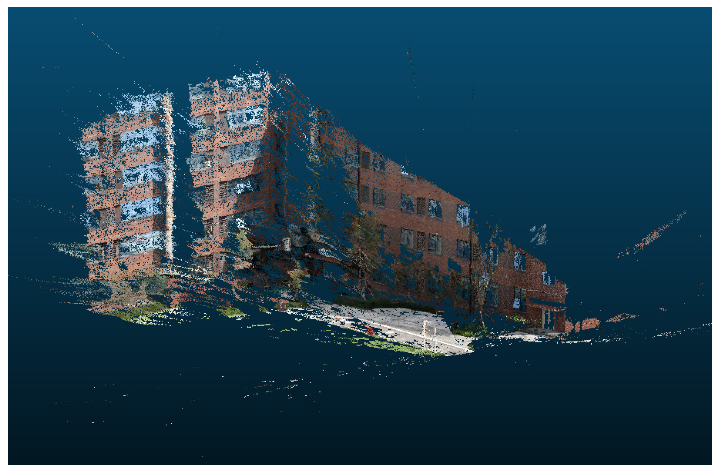
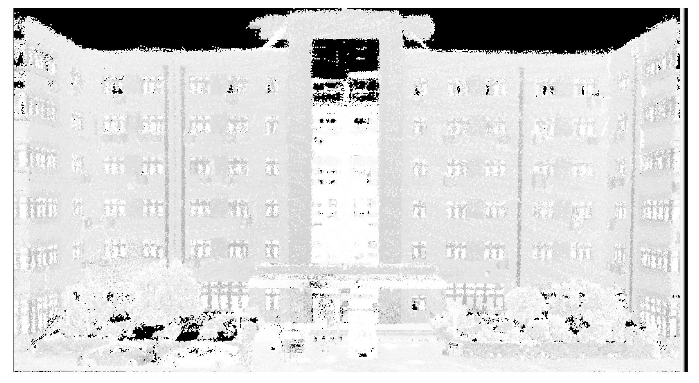
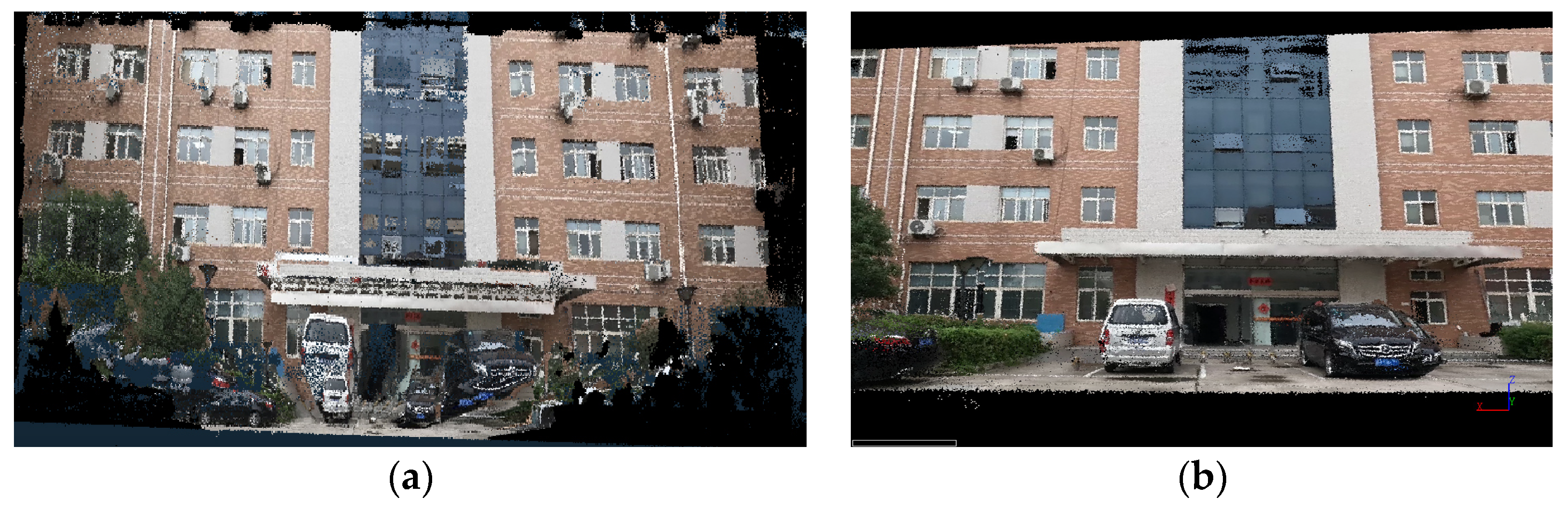
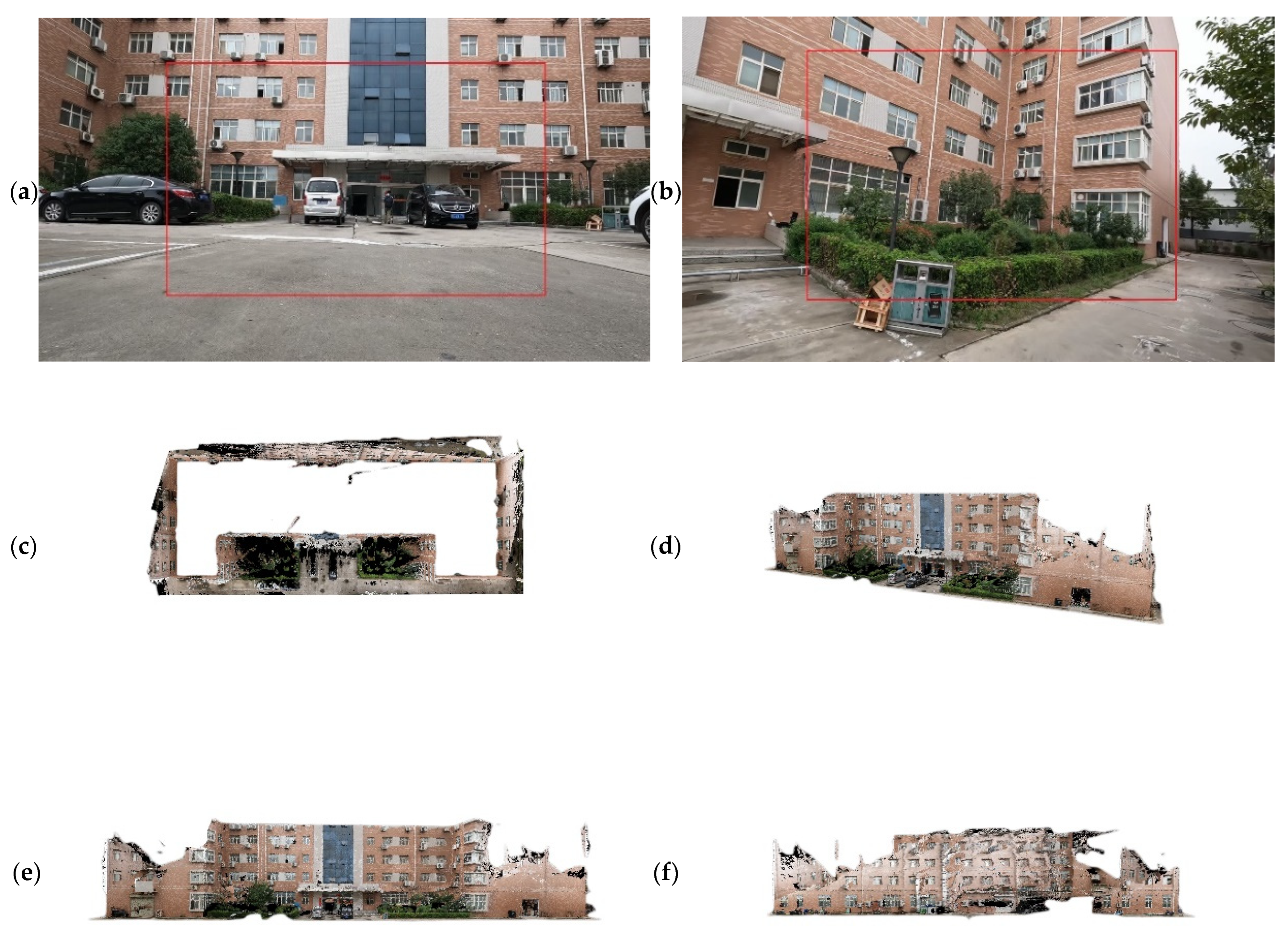
26] further studied this approach by using the 3D-SIFT algorithm to extract feature points from both the LiDAR point cloud and the image-based 3D point cloud, achieving precise registration of the two types of point clouds using the scaling iterative closest point (SICP) algorithm. Obviously, generating an image-based point cloud is a feasible solution, but it requires high-quality image data. In the above-mentioned methods, digital cameras are usually used. In this study, the video images captured by the GoPro camera often suffer from large boundary deformation, unstable interior orientation elements, and blurred pixels. Therefore, problems such as multiple holes and deformation occurred in the image-based point cloud, as shown in Figure 1. It is apparent that the quality of the 3D point cloud generated from the sequential images is poor. Therefore, it is not recommended to use point cloud registration for colorization between these 3D point clouds. Ultimately, we decided to adopt a 1-to-N registration strategy, which means first registering the point cloud with the first image to obtain the exterior orientation elements of the first image. Then, by using relative and absolute orientation, the exterior orientation elements of the remaining sequential images can be obtained.

1.2.1. Obtain the Exterior Orientation Elements of the First Image

It is clear that achieving high-precision automatic registration of a point cloud and the first image has become a key issue. In recent years, scholars have focused more on feature-based registration methods for such problems. Generally, these methods require projecting the point cloud onto a 2D plane to generate an intensity image or a depth image, extracting effective stable and distinguishable feature points from the image, and performing feature matching by calculating the similarity between features [27]. Feature-based registration methods convert the analysis of the entire image into the analysis of a certain feature of the image, simplifying the process and having good invariance to grayscale changes and image occlusions. Fang [28] used different projection methods to project point cloud data and generated a point cloud intensity image. Then, using the SIFT algorithm to extract feature points, the automatic registration between the point cloud intensity image and optical image was achieved. Safdarinezhad et al. [29] used the point cloud intensity and depth to generate an optical consistent LiDAR product (OCLP) and completed automatic registration with high-resolution satellite images using the SIFT feature extraction method. Pyeon et al. [30] used a method based on point cloud intensity images and RANSAC algorithms to perform rough matching and then using the nearest point iterative (ICP) matching, greatly improved on the efficiency of the algorithm. Ding et al. [31] used constraints based on point and line feature to achieve automatic registration of point cloud intensity images and aerial images. Fan et al. [32] extracted corner points of windows and doors from point cloud intensity images and optical images and used the correlation coefficient method to achieve automatic matching of feature points. In the methods above, the conversion of point cloud to image data results in loss of accuracy and requires the point cloud data to be relatively flat with minimal noise. Therefore, in this paper we propose a registration method based on normalized Zernike moments, which is also a point feature-based registration method. Low-order Zernike moments are mainly used to describe the overall shape characteristics of the image [33], while high-order Zernike moments are mainly used to reflect texture details and other information of the image [34]. Normalized Zernike moments can reflect features in multiple dimensions [35], achieving good results even for low-quality images captured by a GoPro action camera and point cloud intensity images.

1.2.2. Obtain the Exterior Orientation Elements of Sequential Images

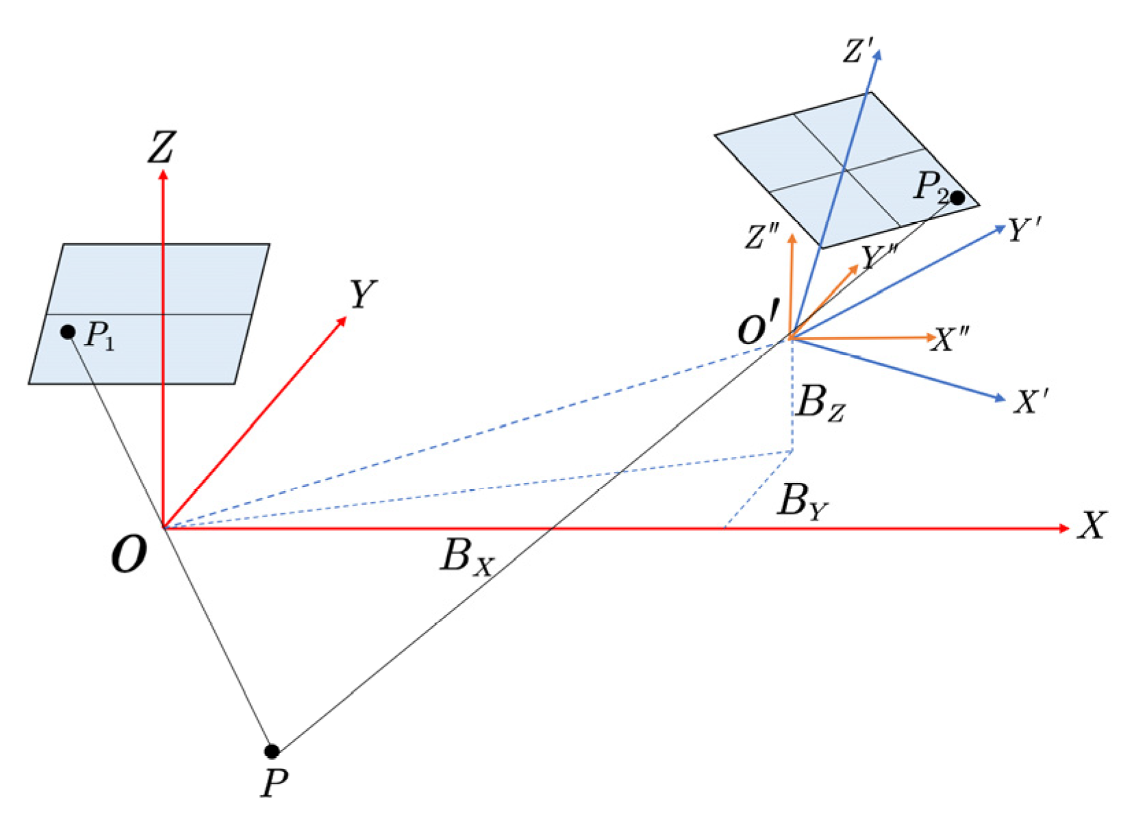
After completing the registration of the first image and the point cloud, relative and absolute orientation are required to transfer the exterior orientation elements for the rest of the sequential images. Relative orientation refers to using an algorithm to calculate the rotation matrix and displacement vector between the right and left image pairs [36] based on several corresponding points in the stereo image pairs, so that the coincident rays intersect [37]. According to this principle, if a continuous relative orientation is performed, the relative positional relationship between all stereo image pairs can be obtained. In traditional photogrammetry, continuous relative orientation is based on initial assumptions, typically assuming the initial values of the three angle elements of the rotation matrix are zero, the first component of the baseline vector is one, and the other two components are replaced with small values, assuming the stereo image pairs are taken under approximately vertical photography conditions [38]. However, in digital close-range photogrammetry, multi-baseline convergence photography is mainly used, such as the GoPro camera used in this paper. Moreover, we obtain video images by capturing video streams. At this time, the relationship between the left and right images in the stereo image pair may be a rotation at any angle, and the forms of angle elements and displacement vectors are complex and diverse. Therefore, traditional relative orientation methods pose difficulty for obtaining correct results [39]. To address this problem, many methods have been proposed. Zhou et al. [40] proposed a hybrid genetic algorithm and used unit quaternions to represent the matrix, which quickly converges without given initial values. Li et al. [41] proposed a normalized eight-point algorithm to calculate the essential matrix and used the Gauss-Newton iteration method to solve the two standard orthogonal matrices produced by decomposing the essential matrix; this improves the accuracy of relative orientation. Therefore, this article intends to use a method based on essential matrix decomposition and nonlinear optimization for relative orientation. Specifically, the essential matrix is first calculated, and its initial value is obtained by performing singular value decomposition [42]. Then, nonlinear optimization is used to obtain an accurate solution.
The stereo model obtained from relative orientation is based on the image-space coordinate system, and its scale is arbitrary. To determine the true position of the stereo model in the point cloud coordinate system, the final step is to determine the transformation relationship between the image-space coordinate system and the point cloud coordinate system, that is, absolute orientation.

1.3. Realistic and Accurate Point Cloud Coloring Method

In the process of coloring the point cloud, a LiDAR point often corresponds to multiple video images. Due to the low quality of the video images used in this paper, problems such as blurry pixels, trailing images and significant deformation exist, making it challenging to perform point cloud coloring that is both realistic and uniform. Vechersky et al. [43] proposed that the color set corresponding to each 3D point follows a Gaussian distribution model. Specifically, the mean and covariance of the weighted Gaussian distribution of the color set are estimated, and the mean value is assigned to the color of the 3D point. Based on this, this paper proposes a Gaussian distribution point cloud coloring method with center area restriction. In simple terms, assuming the color set corresponding to the 3D points follows a Gaussian distribution. Meanwhile, the position information of pixels is statistically analyzed, and only pixels within the central area of the image are selected as valid pixels for coloring. This effectively avoids the phenomenon of blurred edge pixels.
Given the above issues, the chapter arrangement of this article is as follows: Section 1 introduces the current research status of the registration between the point cloud and images. 
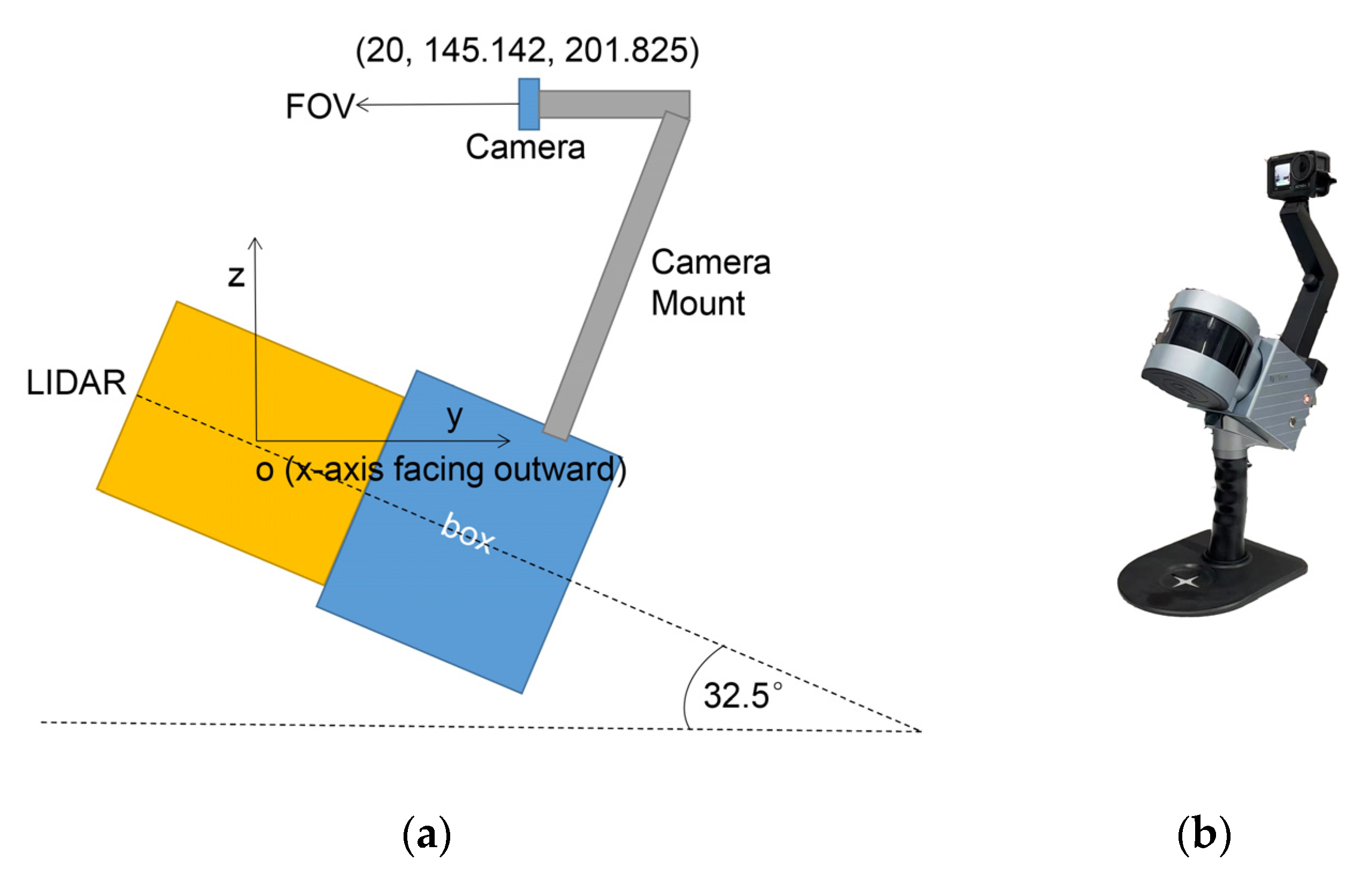
Section 2 briefly introduces the ground mobile LiDAR system and the data used in the experiment. Section 3 focuses on the point cloud coloring method based on video images without POS, and Section 3.1 discusses how to handle the problem of nonlinear distortion of GoPro cameras, mainly using radial and tangential distortion models for correction. The principle of automatic registration based on normalized Zernike moments is described in Section 3.2, from Zernike polynomials to Zernike moments and then to the derivation of normalized Zernike moments. In Section 3.3, we explain how to achieve automatic registration of the point cloud and sequential images, including the selection of the corresponding point matching method, relative orientation based on essential matrix decomposition and nonlinear optimization, and absolute orientation. A detailed description of the steps and strategies for coloring a point cloud is provided in Section 3.4. Section 4 presents experimental results and analysis. Section 5 gives the discussion about the results. 
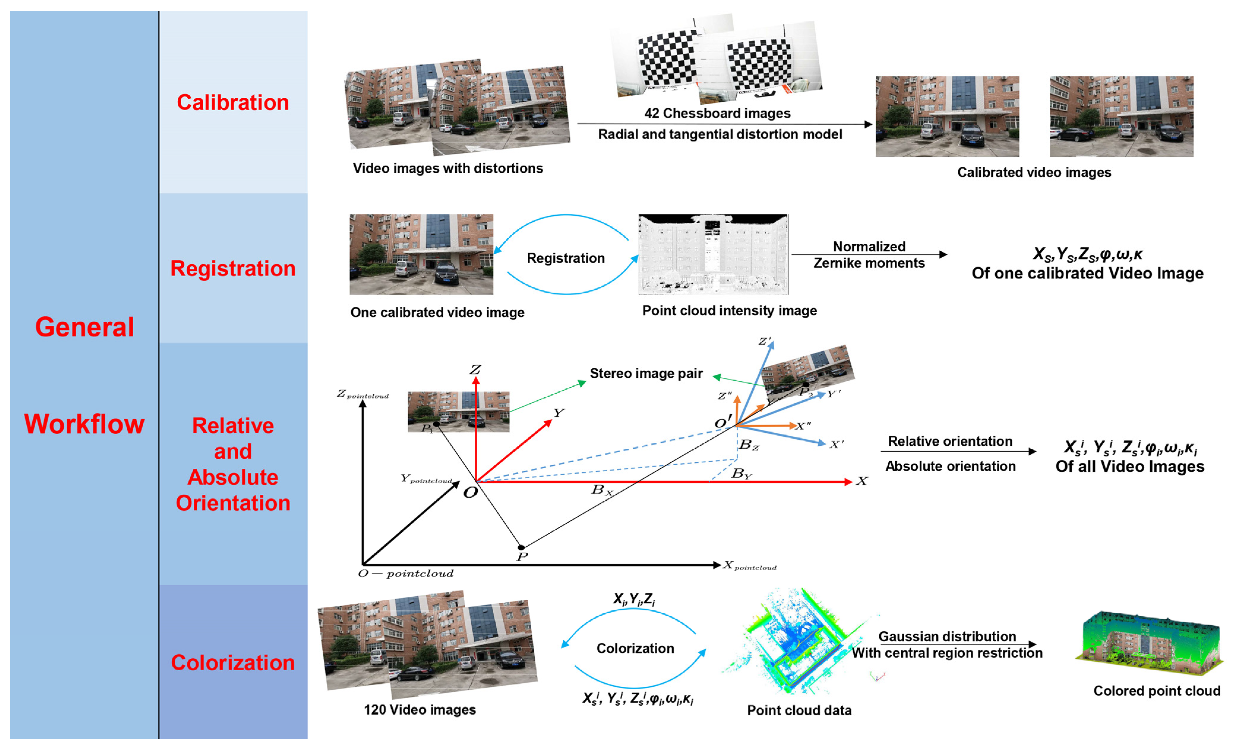
Section 6 summarizes and gives prospects for future work. In summary, the general workflow of the article is shown in Figure 2.

2. System and Data

As shown in Figure 3, we establish a simple ground mobile measurement system integrating a LiDAR and a GoPro camera. Regarding the position where the action camera is fixed, if we take the center of the LiDAR as the origin, the horizontal direction as the y-axis, the vertical direction as the z-axis, and the x-axis perpendicular to the paper and pointing outward, the coordinates of the GoPro camera lens center in the illustrated coordinate system are (20, 145.142, 201.825) in centimeters, and the orientation of the lens field of view (FOV) center is parallel to the y-axis and perpendicular to the x-axis.
The center axis of the LiDAR transmitter is fixed and inclined at an angle of 32.5° to the horizontal ground. During the system’s movement, the LiDAR transmitter will continuously rotate along this central axis. At the same time, the GoPro action camera will also rotate around the camera mount to obtain sufficient data for point cloud coloring. The initial point cloud and some captured video images are shown in Figure 4.

3. Methods

3.1. Camera Calibration

The GoPro camera conforms to the pinhole camera model. According to the principle of the pinhole imaging model, the transformation relationship and its abbreviated form between the image pixel coordinate system and the camera coordinate system is shown as follows:
λ x y 1 = f d x 0 c x 0 f d y c y 0 0 1 X c Y c Z c
k X c = R X w + T
where:
  • p = (x, y): the pixel coordinate of point P in the image plane
  • cx, cy: the coordinate of the principal axis in the pixel coordinate system
  • f: the camera focal length
  • dx, dy: the pixel dimensions
  • λ: the scaling factor
  • Xc, Yc, Zc: the coordinate of point P in the camera coordinate system
Considering that there exists a 3D similarity transformation between the camera coordinate system and the world coordinate system, the transformation formula in abbreviated form are as follows:
k X c Y c Z c = R X w Y w Z w + T
k X c = R X w + T
where:
  • R: the rotation matrix,
  • T: the translation matrix,
  • Xw, Yw, Zw: the world coordinate of point P in space
  • k: the scaling factor between the two coordinate systems
When shooting with a GoPro action camera, significant nonlinear distortion may occur. Figure 5a shows partial images of the chessboard images captured from the video stream. The degree of distortion around the chessboard is still significant, indicating a substantial level of distortion. Figure 5c displays video images where the edges of the straight-line houses are all curved, indicating a significant amount of deformation.
Due to the manufacturing errors in the lens of the action camera, the lens of the camera affects the propagation of light, resulting in radial distortion. The radial distortion can be approximated using the Taylor series expansion of several terms around r = 0, where k1, k2, k3 are radial distortion coefficients and r2 = x2 + y2. Typically, only first-order and second-order terms need to be considered. The normalized coordinates after radial distortion are as follows:
x c o r r e c t e d = x ( 1 + k 1 r 2 + k 2 r 4 + k 3 r 6 ) y c o r r e c t e d = y ( 1 + k 1 r 2 + k 2 r 4 + k 3 r 6 )
In addition to the shape of the camera lens introducing radial distortion, the non-collinear optical centers of the lens groups during assembly introduce tangential distortion, which requires two additional distortion parameters to describe. The tangential distortion coefficients are denoted as p1 and p2. The normalized coordinates after tangential distortion are as follows:
x c o r r e c t e d = x + 2 p 1 x y + p 2 ( r 2 + 2 x 2 ) y c o r r e c t e d = x + 2 p 2 x y + p 1 ( r 2 + 2 y 2 )
It should be noted that Equations (5) and (6) are derived from a general formula and represent two parts of the general formula, respectively: radial distortion and tangential distortion. Based on the distortion described above, we use 42 chessboard images with a size of 12 by 9 and use Zhang’s camera calibration method to obtain the camera parameters and distortion coefficients, as shown in Table 1. The images before and after calibration are shown in Figure 5b,d.

3.2. Registration Based on Normalized Zernike Moments

The essence of registration based on normalized Zernike moments is to perform point feature registration. Firstly, point cloud data needs to be projected to generate a point cloud intensity image, as shown in Figure 6.
Zernike [44] introduced a set of negative functions defined on the unit circle in 1934. These functions have completeness and orthogonality, which enables them to represent any square-integrable function inside the unit disk. The Zernike formula can be expressed as follows:
V p q x , y = V p q ρ , θ = R p q ( ρ ) e x p ( j q θ )
R p q ρ = s = 0 ( p q ) / 2 1 s p s ! ρ p 2 s s ! p + q 2 s ! p q 2 s !
where:
  • ρ: the vector length from point (x, y) to the origin
  • θ: the counterclockwise angle between vector ρ and the x-axis
  • p, q: the order of the Zernike polynomials, ( p q = e v e n , p q )
  • Rpq(ρ): a real-valued radial polynomial.
The Zernike polynomial satisfies orthogonality, which can be expressed as follows:
x 2 + y 2 = 1 V p q * ( x , y ) V n m ( x , y ) d x   d y = π p + 1 δ p n δ q m
Due to the orthogonal completeness of Zernike polynomials, any image within the unit circle can be represented as follows:
f x , y = p = 0 q = 0 Z p q V p q ( ρ , θ )
where Zpq is the Zernike moment, which can construct any high-order moment of an image and has the characteristic of rotation invariance. It is currently widely used as a shape descriptor. Its definition is as follows:
Z p q = p + 1 π x 2 + y 2 = 1 f x , y V p q * ( ρ , θ ) d x   d y
It should be noted that in Equation (11), different coordinate systems are used, with the former being the Cartesian coordinate system and the latter being the polar coordinate system. It is necessary to pay attention to coordinate conversion during computation. For discrete digital images, the integral form can also be written in the form of summation as follows:
Z p q = p + 1 π x y f x , y V p q * ρ , θ , x 2 + y 2 = 1
It can be calculated that the Zernike moments of the image before and after rotation only differ in phase, while the amplitude of the Zernike moments remains unchanged. Therefore, the amplitude of the Zernike moments can be used as a rotation invariant feature of the image. However, Zernike moments only have rotation invariance and not translation and scale invariance, so it is necessary to normalize the image beforehand. The standard moment method is used to normalize an image, and the standard moment is defined as follows:
m p q = x p y q f ( x , y )
x ¯ = m 10 / m 00 y ¯ = m 01 / m 00
The “centroid” of the image can be obtained from the standard moment, and by moving the “centroid” of the image to the center of the unit circle, the translation invariance problem can be solved. In fact, m00 represents the image’s “area”, and by transforming the image with ( x m 00 , y m 00 ) , the purpose of size consistency can be achieved. If the image is transformed with g x , y = f ( x m 00 x ¯ , y m 00 y ¯ ) , the normalized Zernike moments of the final image will be translation, scale, and rotation invariant. In summary, Zernike moments are region-based shape descriptors based on the orthogonalization of Zernike polynomials. The orthogonal polynomial set used is a complete orthogonal set within the unit circle. Zernike moments are complex moments, and the amplitude of the Zernike moments is generally used to describe the shape of an object. The shape features of a target object can be well represented by a small set of Zernike moments. Low-order moments describe the overall shape of the image target, while high-order moments describe the details of the image target. In this paper, high-order moments are used for registration, and the registration steps are as follows:
1.
Project the 3D point cloud onto the point cloud intensity image.
2.
Use the Harris corner detection algorithm to extract corner features from both the point cloud intensity image and the video image.
3.
Treat the region composed of the pixels with the feature points and their neighboring pixels as the “target image”, center the image at the feature point, transform it into the unit circle in polar coordinates, and resample the pixels to the unit circle.
4.
Calculate the zero-order standard moment and the Zernike moments of various orders for the target image, and normalize the Zernike moments.
Z p q = Z p q m 00
5.
Calculate the amplitude of the Zernike moments, which can be used as invariant features, as discussed earlier.
6.
Construct Zernike moment vectors for feature points in the point cloud intensity image and the video image, respectively, using the normalized Zernike moment amplitudes of orders 2 to 4, as shown in Equation (16).
W = ( Z 20 , Z 22 , Z 31 , Z 33 , Z 40 , Z 42 , Z 44 )
7.
First, perform coarse matching of feature points based on Euclidean distance, and then perform matching based on the absolute difference between the two feature point vector descriptors. If the absolute difference is the smallest among all possible results, the matching between feature points is considered successful. Once the matching of corresponding feature points is successful, automatic registration can be performed based on them.
m i n Δ i j = W i W j

3.3. Registration of Point Cloud and Sequential Video Images

3.3.1. Selecting Reliable Corresponding Points

This article adopts a feature-based matching approach for selecting corresponding points. We initially attempted three algorithms, SIFT, ORB, and SURF, and the results and running time are shown in Figure 7 and Table 2. To unify the units, all time units in Table 2 are in milliseconds, which is equivalent to 0.001 s.
For relative orientation, the main considerations are the accuracy and running time of selected corresponding points. Figure 7 shows that all three algorithms contain a considerable number of misaligned points during initial matching, but the lines connecting the corresponding points of ORB and SURF seem to converge more closely in visual representation. According to Table 2, the SURF algorithm has the shortest running time. The 300 ms difference may not be significant, but for the 120 video images used in this paper, this workload needs to be multiplied by 119 times. If there are more images, the time difference would be even greater. Taking into account both the accuracy and time, we ultimately chose to use SURF as the basic algorithm. Naturally, we made some improvements based on the SURF algorithm. The specific steps for corresponding point matching are:
(1)
SURF coarse matching. Firstly, SURF corresponding points coarse matching was conducted on the stereo image pairs.
(2)
Distance restriction. Due to the characteristics of edge blur and trailing in video images, we also applied a distance restriction after SURF. First, calculating the maximum length of the lines connecting the corresponding points, and then only selecting the corresponding points with connecting line length less than 0.6 times the maximum length. This is a method used in remote sensing to filter out corresponding points that are too far apart from each other.
(3)
RANSAC precise matching. To eliminate mismatches of feature points, the RANSAC [45] algorithm was applied after distance restriction to remove incorrect matches.

3.3.2. Relative Orientation Based on Essential Matrix Decomposition and Nonlinear Optimization

The essential matrix [46] contains information about coordinate translation and rotation. In fact, when solving the coordinate transformation matrix, the essential matrix is first solved, and the rotation and translation parameters are obtained by decomposing the essence matrix. This article also goes through this step in relative orientation using the essence matrix decomposition and nonlinear optimization.
First, establishing a relative orientation model as shown in Figure 8. O-XYZ is the spatial rectangular coordinate system with the camera’s photographic center as the origin corresponding to the left image; O′-XYZ′ is the spatial rectangular coordinate system with the camera’s photographic center as the origin corresponding to the right image, and the three rotation angles of O′-XYZ′ coordinate system relative to O-XYZ coordinate system are, respectively, φ, ω, κ; O″-XYZ″ is an artificially established auxiliary spatial rectangular coordinate system, and its three axes are parallel to the three axes of the O-XYZ coordinate system; OO′ is the baseline, and its three displacement components are, respectively, BX, BY, BZ. Suppose there is a ground point P, and the corresponding points in the left and right images are P1 and P2. Suppose the coordinates of P1 in the O-XYZ coordinate system are (x, y, z); the coordinates of P2 in the O′-XYZ′ coordinate system are (x′, y′, z′); the coordinates of P2 in the O″-XYZ″ auxiliary coordinate system are (x″, y″, z″).
From the coplanar condition, the relationship equation can be obtained as follows:
F = B X x x B Y y y B Z z z
x y z = R x y z = r 11 r 12 r 13 r 21 r 22 r 23 r 31 r 32 r 33 x y z
Expanding its determinant yields, and the expressions are as follows:
x y z 0 B Z B Y B Z 0 B X B Y B X 0 r 11 r 12 r 13 r 21 r 22 r 23 r 31 r 32 r 33 x y z = 0
x y z T X R x y z = 0
For any pair of corresponding image points between the stereo images, Equation (21) can also be written as follows:
x i y i z i T X R x i y i z i = 0
[T]XR is the essence matrix, and [T]X contains three translational parameters BX, BY, BZ and the nine direction cosines in R. It can be seen from the formula that it contains the position and posture relationship of the right image with respect to the camera coordinate system.
In the case of a calibrated camera, there are generally two methods to solve for the essence matrix E: (1) Hartley et al. [47] used the normalized eight-point algorithm to solve for the fundamental matrix F using multiple corresponding image points in the left and right images. Then, using the formula E = K1TFK2, the essential matrix is computed. Here, K1 and K2 are the internal parameter matrices of the left and right cameras, respectively. In this paper, they are equal since the same GoPro camera is used for both images. (2) The normalized coordinates of multiple corresponding image points in the left and right images are computed in the camera coordinate system, and then lens distortion correction is applied. Finally, the coordinates are directly substituted into Equation (22) to solve for the essential matrix.
To extract the translation and rotation information contained in the essential matrix, singular value decomposition (SVD) is performed on it:
E = U Σ V T
Then the rotation matrix R and translation vector t can be represented as follows:
R = U W V T / U W T V T , t = α U Z U T / α U Z T U T
W = 0 1 0 1 0 0 0 0 1 , Z = 0 1 0 1 0 0 0 0 0
where α is any nonzero constant. As shown in Equation (24), there are four possible solutions for the rotation matrix R and translation vector t. To determine which solution is correct, we can use the following method: choose a pair of corresponding points and calculate the 3D coordinates of the corresponding object point using each set of R and t. Only the set of R and t that yields positive 3D coordinates for the object point in both left and right camera views (both Z coordinates are positive) is the correct solution. This yields the initial values for the rotation matrix R and translation vector t.
The initial values R, t obtained from the decomposition of the essential matrix often have low accuracy due to the presence of noise in the feature points extracted from the images in close-range photogrammetry. Even with a large number of data points, the initial values can be significantly affected by noise, leading to reduced accuracy. To address this issue, nonlinear optimization is often employed to refine the initial values. Nonlinear optimization plays a significant role in digital close-range photogrammetry, as it is used in camera calibration [48] and bundle adjustment [49]. In this study, we establish a nonlinear optimization objective function based on the coplanarity constraint equation, with the parameters of the three rotation matrix angles (φ, ω, κ) and two translation vectors (BY, BZ) as the optimization variables. We only include two translation vectors as optimization variables because we can set one of the components of the baseline vector BX to 1 for computational convenience, as changes in the length of the baseline vector only result in a proportional scaling of the stereo image pair model. For a pair of corresponding image points, the coplanarity constraint equation is as follows:
F i = f B Y , B Z , φ , ω , k = y i x i B Y x i r 31 + y i r 32 + z i r 33 + x i B Z z i x i r 21 + y i r 22 + z i r 23 + z i B Y y i B Z x i r 11 y i r 12 + z i r 13
By substituting the initial values of the five parameters obtained from the decomposition of the essential matrix and using the Levenberg–Marquardt algorithm [50], multiple iterations of optimization can be performed to obtain the final accurate solution.

3.3.3. Absolute Orientation

A stereo model established through relative orientation of a stereo pair is based on an image-space coordinate system, in which scale is arbitrary. To determine the correct position of the stereo model in the actual object space coordinate system, it is necessary to transform the photogrammetric coordinates of the model points into the object space coordinates, which requires the use of ground control points to determine the transformation relationship between the image-space coordinate system and the object space coordinate system. The above is the concept of traditional absolute orientation. In the study of point cloud coloring in this paper, the above-mentioned object coordinate system becomes the coordinate system of point cloud data, and the ground control points are actually individual 3D points. Therefore, in this paper, absolute orientation is to determine the transformation relationship between the image-space auxiliary coordinate system and the point cloud coordinate system.
Assuming that the coordinates of an arbitrary image point in the image space coordinate system are represented as (X, Y, Z), and the coordinates of the corresponding point in the point cloud coordinate system are represented as (XL, YL, ZL), there exists a spatial similarity transformation relationship between these two coordinates:
X L Y L Z L = λ a 1 a 2 a 3 b 1 b 2 b 3 c 1 c 2 c 3 X Y Z + Δ X Δ Y Δ Z
where:
  • λ: the scale factor,
  • ai, bi, ci: the nine direction cosines
  • ΔX, ΔY, ΔZ: the translation vector
These seven parameters λ, Φ, Ω, K, ΔX, ΔY, ΔZ constitute the spatial similarity transformation, and absolute orientation is essentially the process of solving these seven parameters. Before solving the parameters, it is generally necessary to perform centroid scaling on the coordinates:
X L g = Σ X L n , Y L g = Σ Y L n , Z L g = Σ Z L n X g = Σ X L n , Y g = Σ Y L n , Z g = Σ Z L n
where:
  • XLg, YLg, ZLg: the centroid coordinates of the point cloud
  • Xg, Yg, Zg: the centroid coordinates of the image-space coordinate system
  • n: the number of point cloud control points involved in the calculation
The purpose of centroid scaling is twofold: firstly, to reduce the effective number of decimal places in the coordinates of the model points during the calculation process, in order to ensure the accuracy of the calculation; secondly, by using centroid-scaled coordinates, the coefficients of the normal equations can be simplified, thereby improving the calculation speed.
According to Equation (27), if it is expanded based on Taylor’s theorem, three error equations related to the point cloud coordinates can be obtained. This means that one horizontal control point can produce three error equations, and one vertical control point can produce one error equation. Therefore, when there are more than two horizontal control points and one vertical control point, the seven unknown parameters can be solved by the least squares principle.

3.4. Point Cloud Coloring Method

In this paper, we intend to start from the point cloud to find the corresponding pixels, and then assign values to the point cloud. The reason for choosing to start from the point cloud is that the end of point cloud traversal represents the end of coloring. If we start from the image pixels, it may speed up the coloring process, but it may also result in some point clouds being uncolored, causing discontinuity and missing data in the overall point cloud. Usually, a 3D point in a LiDAR point cloud often corresponds to multiple pixels in multiple images; thus, how to color it correctly based on pixels with poor image quality becomes a critical issue. Therefore, we propose a Gaussian distribution-based point cloud coloring method with a central region restriction. The specific steps are as follows:
1.
Finding pixel sets corresponding to 3D points. Starting from the point cloud, traverse through each 3D point, which corresponds to multiple images. Based on the previous results, the pixel coordinates corresponding to each 3D point can be calculated from the images. The nearest neighboring pixels are selected as the corresponding pixel of the 3D point, and their color and position information are recorded.
2.
Applying central area restriction. Based on the location information gathered in step 1, only pixels within the central area of the image are considered valid for coloring the point cloud.
3.
Coloring. We assume that for a valid pixel color set corresponding to a 3D point, any of the RGB channels follow a Gaussian distribution. We estimate the mean of each channel’s Gaussian distribution and consider it as the color value of that channel. Finally, we assign the RGB color to the 3D point.
4.
Repeat steps 1, 2 and 3 until all 3D points have been processed.

4. Results

4.1. Registration Based on Normalized Zernike Moments

Registration results based on the collinearity equation and normalized Zernike moments are shown in Table 3 and Table 4 and Figure 9. Table 2 displays the 3D coordinates of point cloud control points and registration accuracy of the collinearity equation. Table 3 displays the 3D coordinates of several Harris feature points of the point cloud and registration accuracy of normalized Zernike moments. Figure 9 is a screenshot of the colored point cloud obtained from the registration result, which can also serve as a reference image for the registration accuracy.

4.2. Corresponding Point Matching

In this article we uniformly adopt the SURF algorithm with distance restriction and RANSAC to select corresponding points. We randomly select a stereo image pair (28–29) as an example, and the result is shown in Figure 10.
As shown in Figure 10a, there are 400 corresponding points selected by the SURF coarse matching, among which there are many mismatched points and corresponding points located at the edges of the image. After applying distance restriction, the number of corresponding points decreased from 400 to 173, as shown in Figure 10b. The corresponding points located at the edges of the image were reduced, but there were still many mismatches. After applying RANSAC, as shown in Figure 10c, the number of corresponding points dropped sharply from 173 to 72. The mismatches were mostly eliminated after the RANSAC process. It can be seen that after these three steps, the accuracy of the corresponding points is relatively high, and they are mostly located in the central area of the image, which meets the requirements well. However, after obtaining a series of corresponding points, selecting how many pairs for relative orientation becomes a problem. The number and accuracy of the selected corresponding points will definitely affect the accuracy of relative orientation. Therefore, we statistically analyze the data in Figure 11 and Table 5. Figure 11 shows how the number and accuracy of the corresponding points affect the accuracy of the vertical parallax of relative orientation by selecting the top 10, 15, 20, 40, 60, 80 and 100 corresponding points. Table 5 summarizes the situations of eight stereo image pairs.
In general, selecting corresponding points with accuracy in the top 10 to 15, 20, or even 100 has a decreasing impact on the accuracy of relative orientation in terms of vertical parallax. This is because corresponding points with lower accuracy definitely result in poorer results. However, it is not necessarily true that selecting corresponding points with higher matching accuracy will lead to better results in relative orientation. For example, the relative orientation results obtained by selecting corresponding points with matching accuracy in the top 10 were not as good as those obtained by the top 15, and the results obtained by the top 15 were not as good as those obtained by selecting the top 20. It is speculated that nonlinear distortion, trailing, and blurred pixels in the video images used in this study may cause significant errors when selecting fewer corresponding points. So, selecting more corresponding points can help to distribute these errors more evenly. However, more corresponding points means lower matching accuracy. Therefore, in this study, we ultimately decided to select corresponding points with matching accuracy in the top 20 for relative orientation.

4.3. Relative Orientation

The results of relative orientation based on essential matrix decomposition and nonlinear optimization are shown in Figure 12. Figure 12a–c show the results of three stereo image pairs, with the left images being the left image of the stereo pair and the right images being the right image of the stereo pair. The results indicate that this method yields good results for different situations such as: small rotation angles (Figure 12a), large rotation angles (Figure 12b) and both large rotation angles and displacements (Figure 12c).

4.4. Absolute Orientation

Absolute orientation is a 3D spatial similarity transformation between the relative orientation stereo model coordinate system and the point cloud coordinate system. Therefore, the accuracy of absolute orientation mainly depends on the accuracy of the relative orientation stereo model and the accuracy of corresponding points between the two coordinate systems. At the same time, since the sequential images are obtained by capturing the video stream, the captured images under the motion state will cause blur in some parts of the images, further leading to measurement errors. Therefore, the main error sources of absolute orientation come from the relative orientation stereo model error and the measurement error of point cloud control points. For the accuracy of absolute orientation, we use the difference between the coordinates obtained by absolute orientation and the coordinates of the corresponding control points in the point cloud and the mean squared error (MSE) of each relative orientation element as the evaluation standards. The results are shown in Table 6.

4.5. Point Cloud Colorization

The results of the colored point cloud are shown in Figure 13. Figure 13a,b demonstrate the importance of center region restriction in the Gaussian distribution coloring method. It is evident that even after calibration, pixel blurring and uncorrected phenomena still occur in the edge regions of the video image. Therefore, the center region restriction is critical, and only the pixels within the red box are considered qualified and can be used to color the point cloud. Figure 13c–g shows the point cloud coloring results, including the top view, side view, front view, back view and total view. In Figure 13g, the blue and green parts represent uncolored points. Due to the limitations of the video imaging range, high-altitude walls, car roofs, treetops, and roofs are all uncolored.

5. Discussion

In the beginning of the discussion, we want to explain that we have tried a cheap IMU for registration [51,
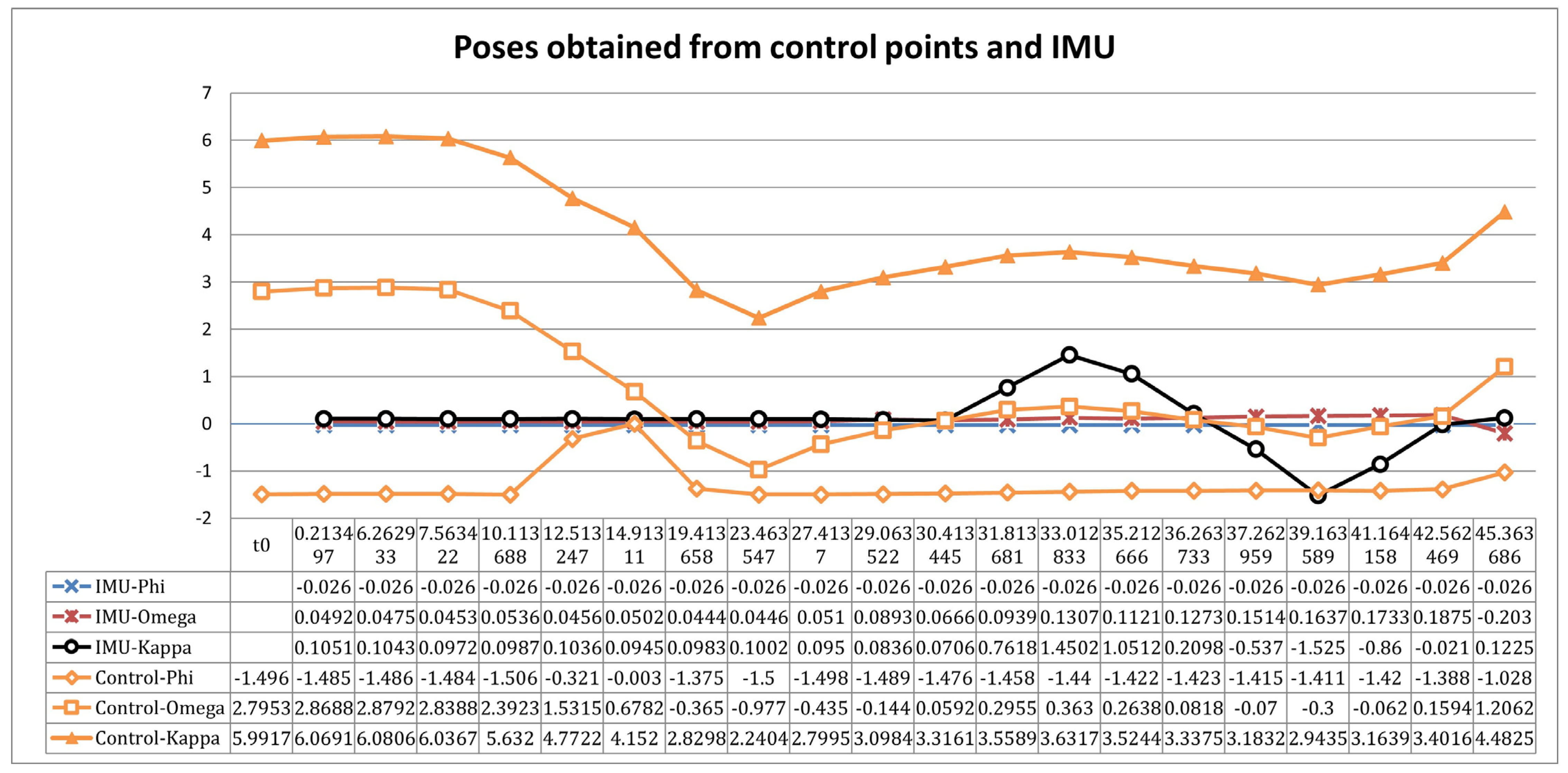
52] and why we finally decided not to use it. Our idea was to install the IMU on the laser to measure the rotation and the scanning angle of the laser. However, the IMU could only provide pitch and heading angles, while the camera’s roll angle could not be obtained. In this case, we assumed that the camera’s roll angle was constant and stable, but it was difficult to achieve this state in actual experiments. We also attempted to use the pitch and heading angles of the IMU for computation, but the resulting poses of the image had a large error compared to the manually selected control points of the images. As shown in Figure 14, we compared the poses of 20 images obtained from manually selected control points and calculated from the IMU. The results indicate that the IMU has a significant error, which is why we ultimately did not integrate the IMU.
To achieve the automatic coloring of point cloud in our system, we went through several steps: (1) Camera calibration. (2) Registration based on normalized Zernike moments. (3) Corresponding point matching with distance restriction. (4) Relative and absolute orientation. (5) Gaussian distribution point cloud coloring with center region restriction. In the experimental process, each step is crucial, and the accuracy of each intermediate result will directly or indirectly affect the subsequent results.
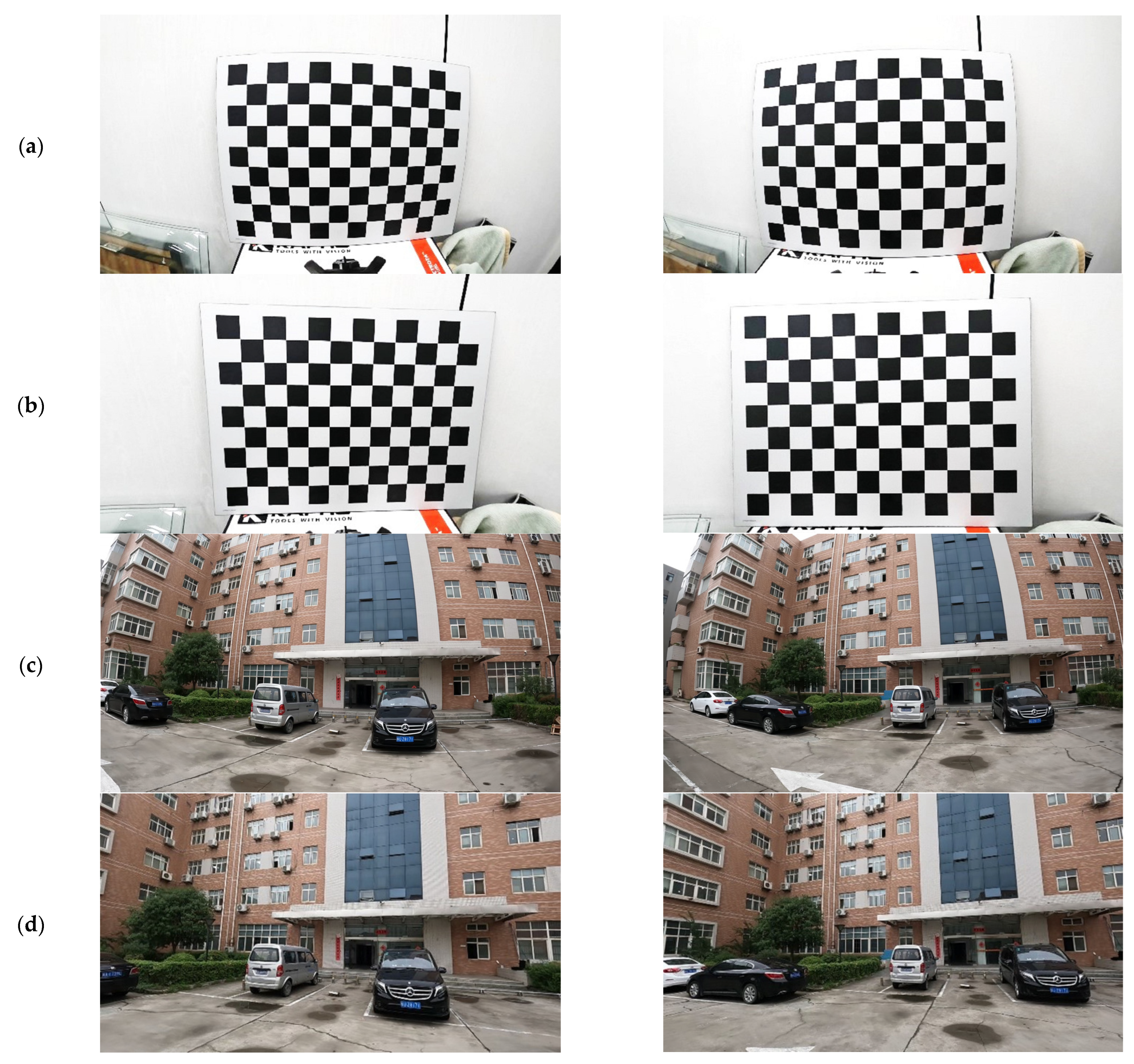
As the video images used in this paper were captured from a GoPro camera during the mobile measuring process, they suffer from significant distortion. Therefore, Zhang’s camera calibration method was used to correct the nonlinear distortion. According to Figure 5a–d, it can be seen that the edges of the chessboard and the edges of the house are well corrected. However, the limitation of this method is that it only considers the tangential and radial distortion models which have a greater impact on distortion but does not consider other types of distortion [5,6,7,8].
Registration based on normalized Zernike moments is actually registration based on point features [27,28,29,30,31,32], and its accuracy mainly depends on the selection of feature points and the descriptor of the feature region. When selecting feature points, as the registration area is the front of the house with many windows and grasses, this paper uses the Harris operator to extract corner points as feature points. Due to the phenomenon of blurred edges in video images, normalized Zernike moments are used to describe the feature region. Low-order Zernike moments describe the overall shape characteristics of the image, while high-order Zernike moments reflect the texture details of the image [33,34,35]. Normalized Zernike moments are invariant to rotation, translation, and scaling and can serve as the determining factor for registration. According to Figure 9, the registration results based on the collinearity equation are generally acceptable, but there are still some areas around the edges where registration is not accurate, which is due to the system’s mobile measurements, resulting in blurry edges and distortions in video images. On the contrary, normalized Zernike moments utilize information from neighboring pixels when extracting features, which can reflect features in more dimensions and describe the texture details of the image. Therefore, the registration results based on normalized Zernike moments are better. According to Table 3 and Table 4, the registration accuracy based on normalized Zernike moments is around 0.5 pixels, which is 1–2 pixels higher than that of the registration accuracy of collinearity equation. However, due to the low accuracy of the video images, direct registration between an image-based point cloud and a laser point cloud cannot be achieved [25,26]. In addition, to avoid complex computations and long running times, this paper only uses normalized Zernike moments of 2–4 orders as the vector descriptor of the region, so further progress can be made from higher orders.
Due to the lack of POS and IMU in our system, we cannot directly obtain the exterior orientation elements of the images. Therefore, we adopt a registration strategy from 1 to N, which is to transmit exterior orientation elements through relative and absolute orientation [36,37]. The premise of relative orientation is the matching of corresponding points. According to 
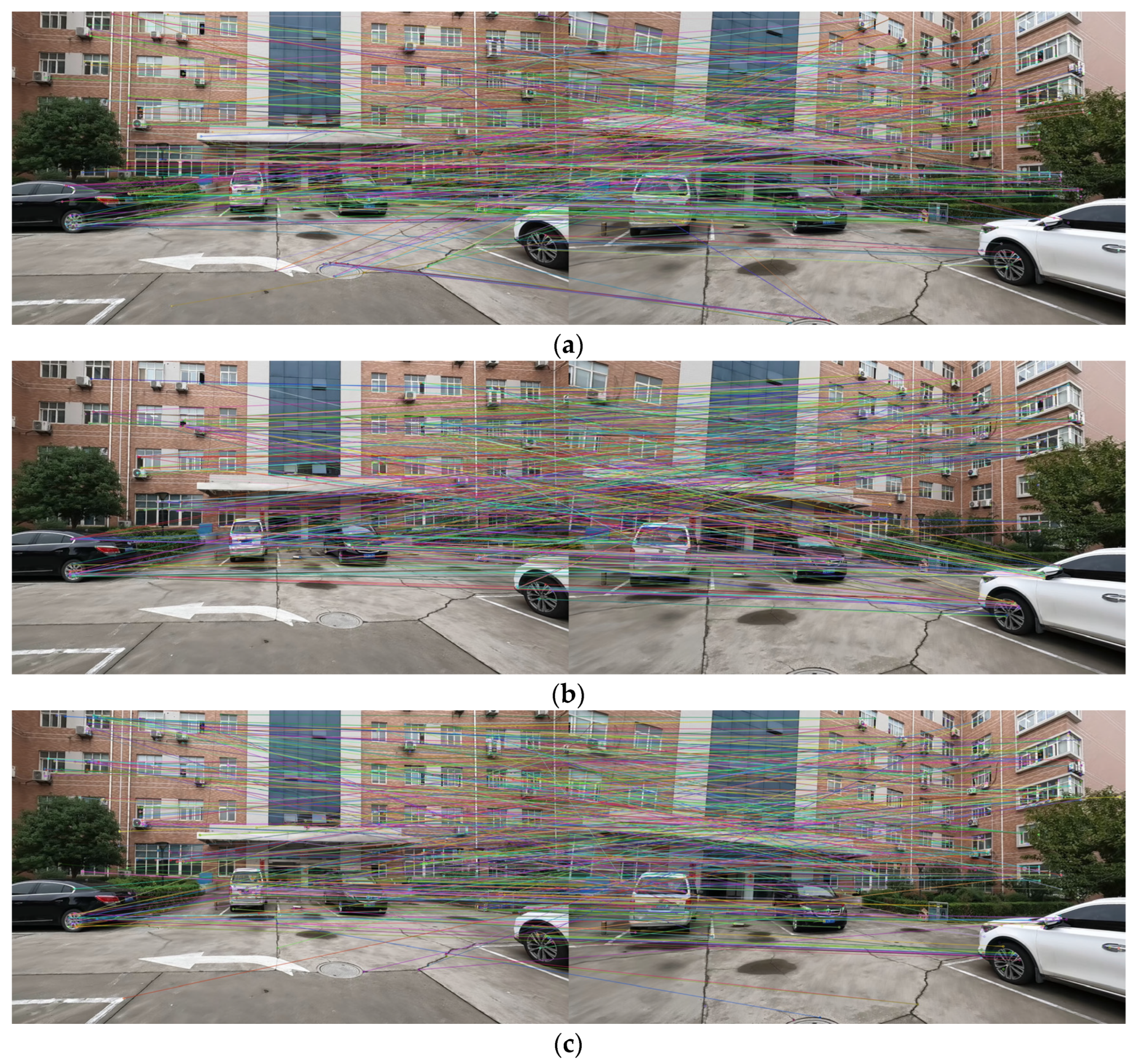
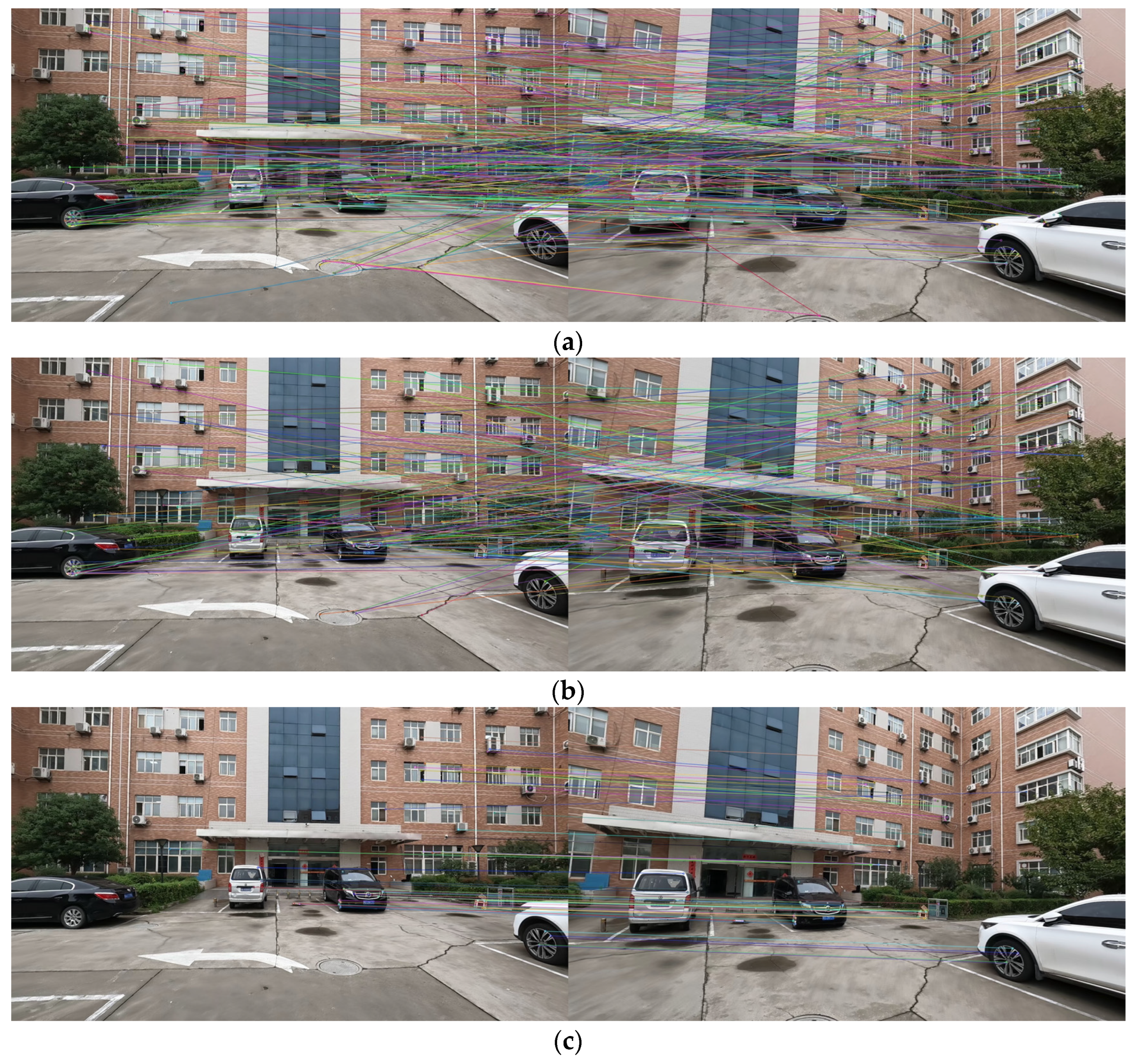
Figure 7, considering both accuracy and quantity, we choose the SURF algorithm. Due to phenomena such as edge blurring in video images, it is necessary to avoid selecting corresponding points in the edge regions. Therefore, we propose a SURF matching method with distance restrictions. According to Figure 10a,b, after applying distance restrictions, the number of corresponding points located on the edge of the image is significantly reduced, but there are still many mismatched points in the edge region. After performing RANSAC, according to 
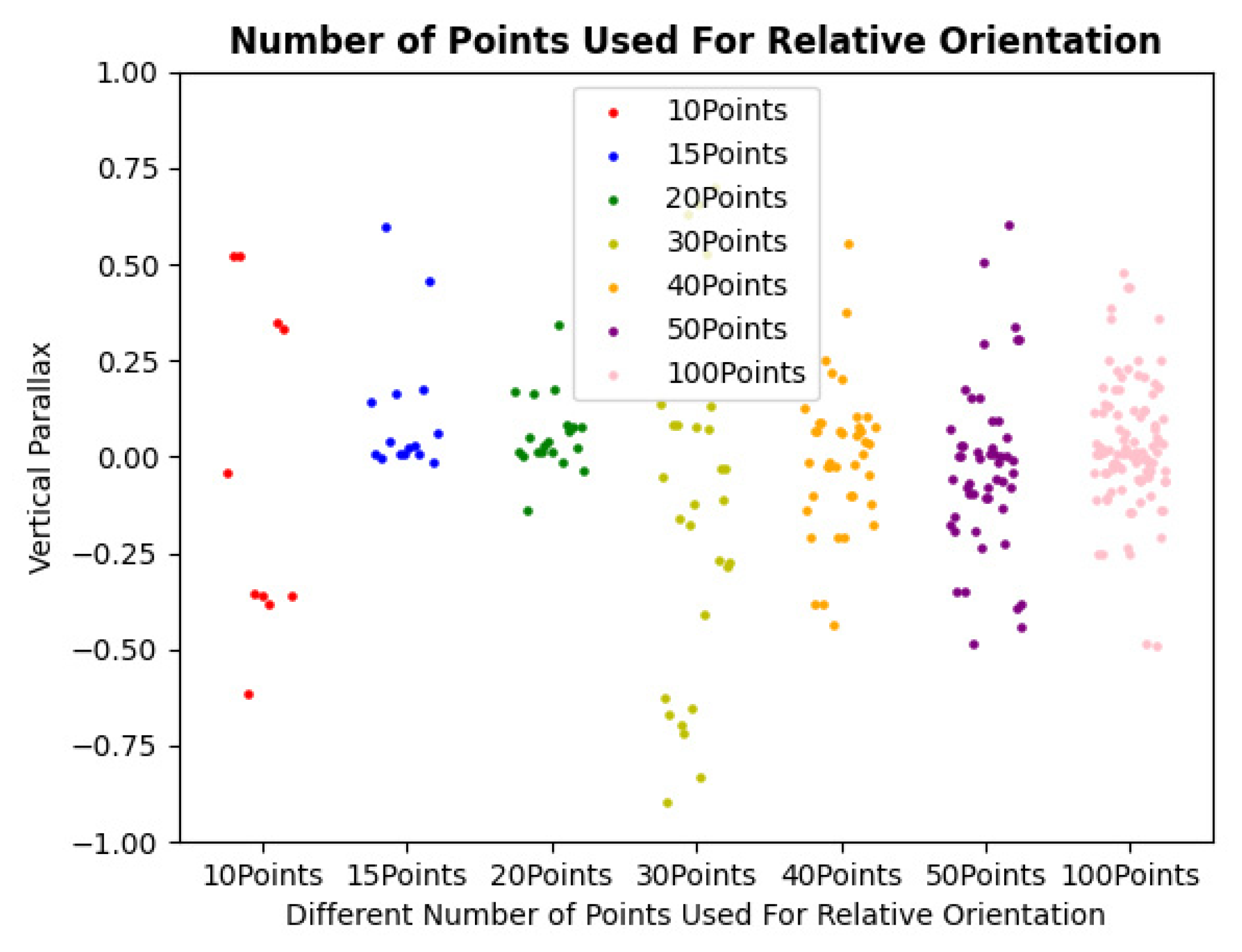
Figure 10c, high-precision corresponding points located in the central region of the image are obtained. In addition, we separately analyzed the influence of the top 10, 15, 20, 30, 40, 50, and 100 corresponding point pairs on relative orientation. As shown in Figure 11 and Table 5, selecting the top 20 points yields the smallest vertical parallax and highest accuracy. One area for improvement is that, for convenience, we uniformly selected the top 20 points for relative orientation for each stereo image pair. However, theoretically, each stereo image pair has its optimal number of corresponding points, but this would increase complexity and computation time.
After the above steps, the registration between all images and point clouds is completed. Here, we explain why this paper did not choose the method of registration based on semantic features. Firstly, registration based on semantic features has its own advantages, including better robustness and resistance to image noise [53]. However, registration based on semantic features requires pre-training, a large amount of data, classification and recognition of objects in advance, and high-quality images. For this paper, which has video images with blurry edges, registration based on semantic features is not suitable. The registration methods used in this paper, including registration based on normalized Zernike moments, SURF, and relative orientation, are all based on point and point features. Our focus has always been on high-precision corresponding points with precise geometric positions. Even with low-quality video images, a good, colored point cloud can be obtained. Therefore, this paper did not adopt the method of registration based on semantic features.
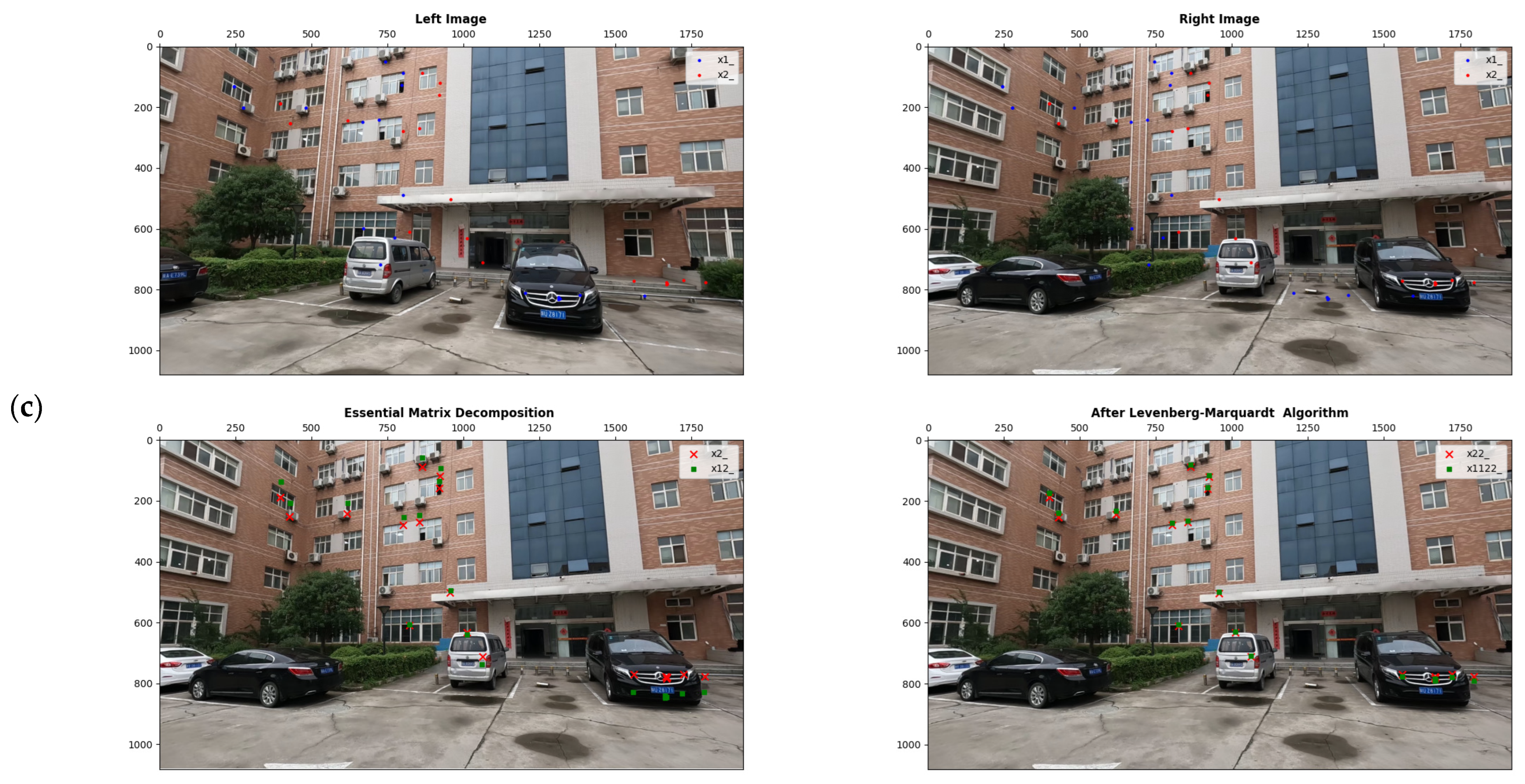
The essence of relative orientation is to solve the essential matrix [39,40,41]. Based on this, this paper uses essential matrix decomposition and nonlinear optimization to perform relative orientation [42], according to 
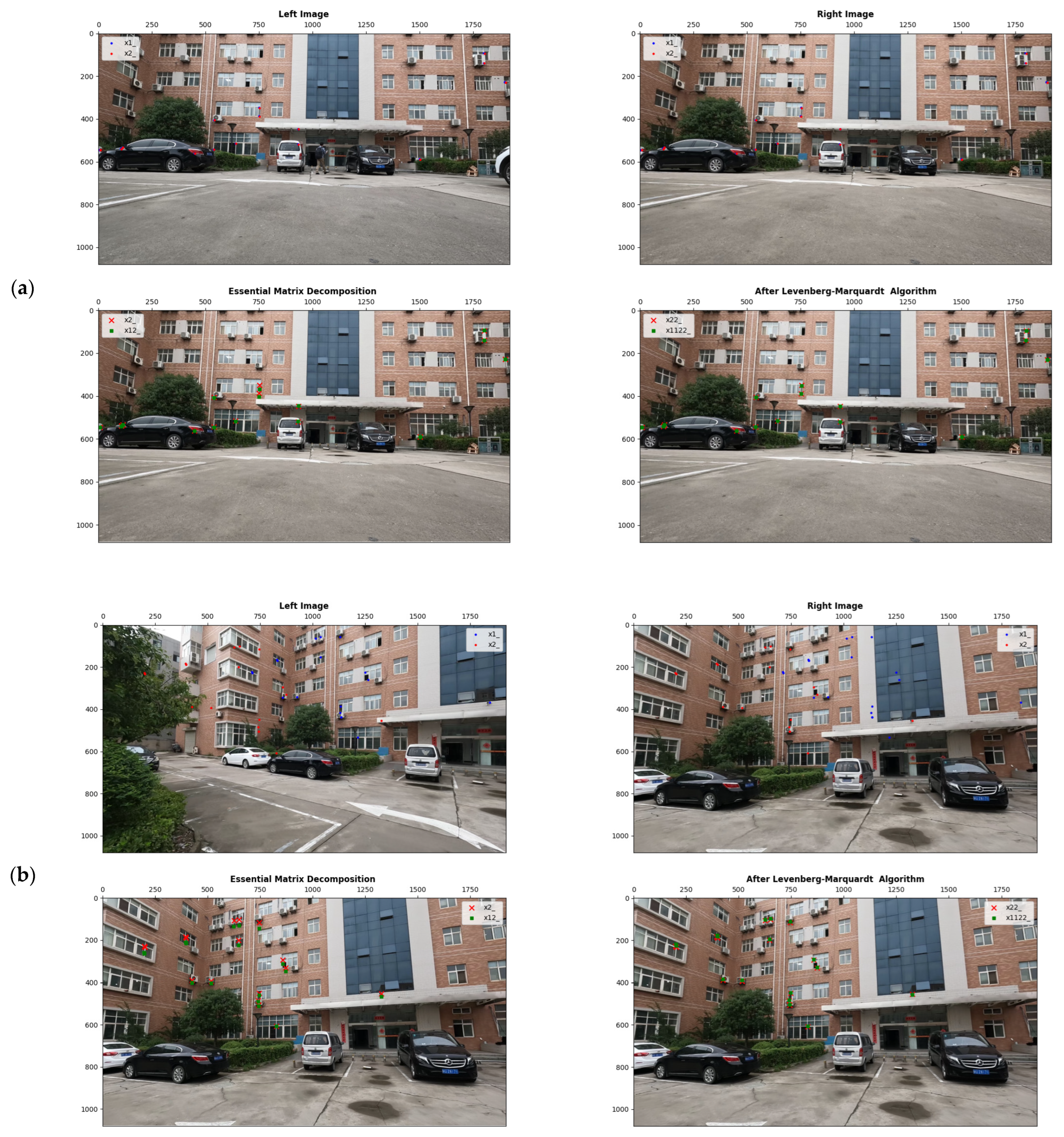
Figure 12. The method used in this paper has stronger applicability than traditional relative orientation. Traditional relative orientation is based on the assumption of approximately vertical photography and can only converge to the correct result when the rotation angle of the image is small. According to Figure 12a–c, good results can be obtained for general cases, large rotation angles, and large displacement. There are mainly two aspects to demonstrate the high accuracy: (1) Based on visual interpretation, after relative orientation, the corresponding points of the left and right images have almost completely coincided with each other. For different situations, the corresponding points can still coincide well with each other. (2) According to Table 4, when selecting the Top 20 corresponding points for relative orientation, the vertical parallax of the stereo image pair model is less than one pixel. At the same time, we can also see the importance of non-linear optimization. After nonlinear optimization, the corresponding points of the left and right images are almost coincident. Absolute orientation is required after relative orientation, and the accuracy of absolute orientation depends on the accuracy of the stereo image model and the precision of control point selection. With the prerequisite of accurate previous steps, good results can also be obtained in absolute orientation. As shown in Table 6, we use 15 image points from a stereo image pair for absolute orientation, and the MSE of X, Y, and Z are all at the centimeter level.
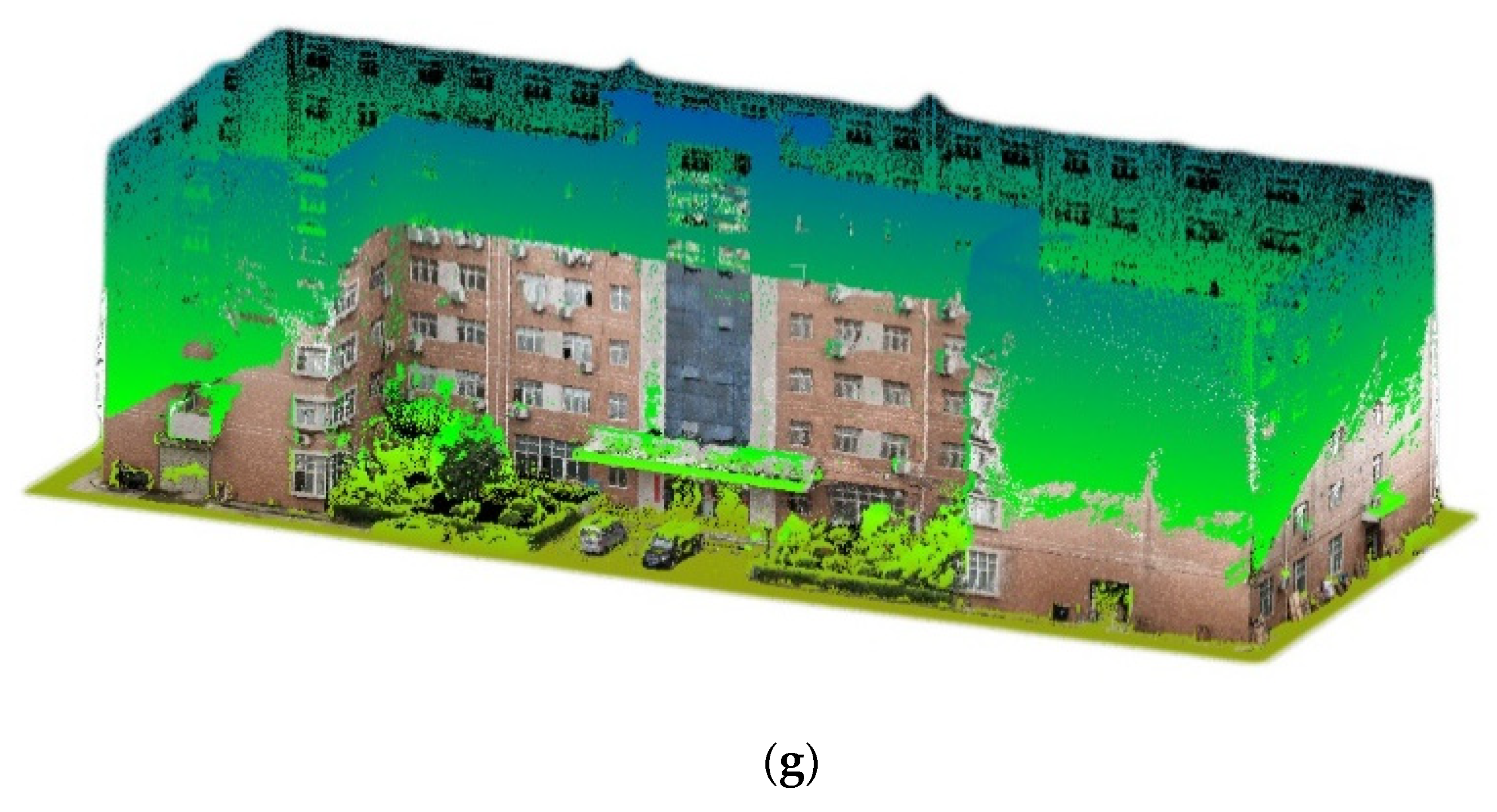
The phenomenon of edge blurring in video images has been present throughout the entire experimental process and cannot be ignored, even in the final step of point cloud coloring. Therefore, this paper adopts a Gaussian distribution point cloud coloring method with central region restrictions. According to Figure 13g, the point cloud coloring results have overall high accuracy. The textures of buildings are very clear, and the corners of the houses are also very obvious. In addition, targets such as windows, grass, trees, and vehicles can be clearly distinguished. The biggest drawback is that due to the limited range of the video images, the high-altitude point cloud of buildings, the crowns of trees, and the roofs of cars are not colored. Therefore, the next research direction is how to colorize point cloud with high-altitude to obtain a complete, colored point cloud.
Finally, it is declared that the entire process of this article is implemented using the C++ programming language. Figure 11 and Figure 12 were visualized using Python. We will also provide the running time for each step, as shown in Table 7. To unify the units, all time units in Table 6 are in milliseconds, which is equivalent to 0.001 s. In addition, in Table 6, the calibration time refers to the total time it took to calibrate 42 chessboard images, while the time for corresponding point matching, essential matrix decomposition, and nonlinear optimization all refer to the processing time for one stereo image pair.

6. Conclusions

In this article, we propose an automatic point cloud colorization method for a ground measurement LiDAR system without POS. The system integrates a LiDAR and a GoPro camera and has the characteristics of simplicity, low cost, light weight, and portability. As a loosely coupled integrated system, it has the possibility of industrial mass production and can complete automatic point cloud registration and colorization without POS. The method mainly consists of four steps: calibration, registration, relative orientation and absolute orientation, and colorization. (1) To solve the problems of video image motion blur, pixel blur, and nonlinear distortion of GoPro, in preprocessing we use radial and tangential distortion models to correct the GoPro camera based on 42 chessboard images extracted from video streams. After calibration, it can be seen that the edges of the chessboard and the edges of the house are well corrected. (2) To achieve image sequence registration without POS, this article proposes a 1-N registration strategy. We only perform registration between the first video image and the point cloud and use the relative and absolute orientation to transfer the exterior orientation elements to all sequential images. In registration, a method based on normalized Zernike moments is proposed to achieve high registration accuracy even for blurry video images. The registration based on Normalized Zernike moments has an error of only 0.5–1 pixel, which is far higher than collinearity equations. (3) In the corresponding point matching, this article proposes a SURF corresponding point matching method with distance restriction and RANSAC to eliminate corresponding points with blurred edges and mismatches. We select the top 20 corresponding points for relative orientation based on essential matrix decomposition and nonlinear optimization. The parallax of the stereo image pair model is less than one pixel. (4) Finally, in the point cloud colorization, we propose a Gaussian distribution coloring method with a central region restriction, which can complete point cloud colorization realistically and evenly. In the colored point cloud, the textures of various objects such as buildings, cars and trees are very clear. Based on the results of the final point cloud colorization, we prove the feasibility of the method proposed in this article, which provides a reference for the future point cloud colorization of ground mobile measurement LiDAR systems.
For the blurry video images, the reliability of corresponding points is questionable. Therefore, the following research will be carried out: (1) Using features such as tie-line or parallel-line attributes to achieve registration between point cloud data. (2) Establishing a joint calibration [54] field for the motion camera and LiDAR to solve the rigid combination between them and achieve automatic matching of both data. (3) Starting from improving the methods of relative and absolute orientation, adopting more accurate and faster methods. For example, Li et al. [55] proposed a hybrid conjugate gradient algorithm for large-angle stereo image relative orientation, which is independent of initial values and has high accuracy and fewer iterations. Deng et al. [56] proposed an absolute orientation algorithm based on line features, which reduces the need for control points and tie points and improves accuracy and stability through joint adjustment. (4) As the scenario in this article is a closed small scene area, we did not use GPS. After relative orientation, we introduced parameters such as scale factor and rotation angle to control the camera’s offset through the laser point cloud—absolute orientation between images and point clouds. Even though the final coloring accuracy is acceptable, there is definitely a cumulative system error when performing continuous relative orientation, and GPS can correct these system errors by providing absolute positions. This is a current weakness of our article. For future experiments, perhaps in large-scene applications, we will add GPS to the system, which is also an important direction for our future research.

Author Contributions

All authors contributed in a substantial way to the manuscript. Software, C.Q.; writing—original draft, J.X. and J.W.; writing—review & editing, C.Y. and H.M. All authors have read and agreed to the published version of the manuscript.

Funding

This research was funded and supported by National Key R&D Program of China grant number (2018YFB0504500), National Natural Science Foundation of China grant number (41101417) and National High Resolution Earth Observations Foundation grant number (11-H37B02-9001-19/22).

Data Availability Statement

The data presented in this study are available on request from the corresponding author. The data are not publicly available due to privacy.

Conflicts of Interest

The authors declare no conflict of interest.

References

  1. Zhang, J. Deformation Monitoring of Wooden Frame Relics Based on 3D Laser Scanning Technology. Beijing Surv. Mapp. 2018, 32, 768–772. [Google Scholar] [CrossRef]
  2. Zhang, J.; Jiang, W.S. Registration between Laser Scanning Point Cloud and Optical Images: Status and Trends. J. Geo-Inf. Sci. 2017, 19, 528–538. [Google Scholar]
  3. Yang, B.W.; Guo, X.S. Overview of Nonlinear Distortion Correction of Camera Lens. J. Image Graph. 2005, 10, 269–274. [Google Scholar] [CrossRef]
  4. Duane, C.B. Close-range camera calibration. Photogramm. Eng. 1971, 37, 855–866. [Google Scholar]
  5. Melen, T.; Balchen, J.G. Modeling and calibration of video cameras. Proc. SPIE 1994, 2357, 569–577. [Google Scholar] [CrossRef]
  6. Heikkilä, J.; Silvén, O. A four-step camera calibration procedure with implicit image correction. In Proceedings of the IEEE Computer Society Conference on Computer Vision and Pattern Recognition, San Juan, PR, USA, 17–19 June 1997; pp. 1106–1112. [Google Scholar] [CrossRef]
  7. Fraser, C.S. Digital camera self-calibration. Isprs J. Photogramm. Remote Sens. 1997, 52, 149–159. [Google Scholar] [CrossRef]
  8. Hu, H.; Liang, J.; Tang, Z.Z.; Guo, X. Global calibration for muti-camera videogrammetric system with large-scale field-of-view. Opt. Precis. Eng. 2012, 20, 369–378. [Google Scholar] [CrossRef]
  9. Gao, Z.Y.; Gu, Y.Y.; Liu, Y.H.; Xu, Z.B.; Wu, Q.W. Self-calibration based on simplified brown non-linear camera model and modified BFGS algorithm. Opt. Precis. Eng. 2017, 25, 2532–2540. [Google Scholar]
  10. Zou, P.P.; Zhang, Z.L.; Wang, P.; Wang, Q.Y.; Zhou, W.H. Binocular Camera Calibration Based on Collinear Vector and Plane Homography. Acta Opt. Sin. 2017, 37, 244–252. [Google Scholar] [CrossRef]
  11. Xie, Z.X.; Chi, S.K.; Wang, X.M.; Pan, C.C.; Wei, Z. Calibration Method for Structure-Light Auto-Scanning Measurement System Based on Coplanarity. Chin. J. Lasers 2016, 43, 182–189. [Google Scholar] [CrossRef]
  12. Yu, J.P.; Lin, J.H.; Zhan, S.H.; Yao, N.W. A Comparative Study of Close-Range Image Feature Points Matching Method. J. Guangdong Univ. Technol. 2018, 35, 56–60. [Google Scholar] [CrossRef]
  13. Harris, C.G.; Stephens, M.J. A Combined Corner and Edge Detector. Alvey Vis. Conf. 1988, 15, 10–5244. [Google Scholar] [CrossRef]
  14. Lowe, D.G. Distinctive Image Features from Scale-Invariant Keypoints. Int. J. Comput. Vis. 2004, 60, 91–110. [Google Scholar] [CrossRef]
  15. Bay, H.; Tuytelaars, T.; Gool, L.V. SURF: Speeded Up Robust Features. Eur. Conf. Comput. Vis. 2006, 3951, 404–417. [Google Scholar] [CrossRef]
  16. Rublee, E.; Rahaud, V.; Konolige, K.; Bradski, G. ORB: An efficient alternative to SIFT or SURF. In Proceedings of the 2011 International Conference on Computer Vision, Barcelona, Spain, 6–13 November 2011; pp. 2564–2571. [Google Scholar] [CrossRef]
  17. Zeng, F.Y.; Gu, A.H.; Ma, Y.J.; Xiang, H.D. Analysis and Comparison of several kinds of Feature Points Extraction Operator. Mod. Surv. Mapp. 2015, 38, 15–18. [Google Scholar] [CrossRef]
  18. Liu, D.; Wang, Y.M.; Wang, G.L. Feature Point Extraction of Color Digital Image Based on Harris Algorithm. J. Beijing Univ. Civ. Eng. Archit. 2008, 24, 26–29. [Google Scholar] [CrossRef]
  19. Cui, L.; Li, C.; Li, Y. Implementation and Analysis of Harris Algorithm and Susan Algorithm. Comput. Digit. Eng. 2019, 47, 2396–2401. [Google Scholar] [CrossRef]
  20. Jia, F.M.; Kang, Z.Z.; Yu, P. A SIFT and Bayes Sampling method for Image Matching. Acta Geod. Cartogr. Sin. 2013, 42, 877–883. [Google Scholar]
  21. Cao, N.; Cai, Y.Y.; Li, X.Y.; Li, L. Research on Feature Point Automatic Matching Method for High-resolution Remote Sensing Images. Geospat. Inf. 2022, 20, 9–13. [Google Scholar] [CrossRef]
  22. Zhang, Y. Research on Point Feature Matching Algorithms of UAV Remote Sensing Images. PLA Inf. Eng. Univ. 2015, 102, 102456. [Google Scholar]
  23. Rosten, E.; Drummond, T. Machine learning for high-speed corner detection. In Proceedings of the Computer Vision–ECCV 2006: 9th European Conference on Computer Vision, Graz, Austria, 7–13 May 2006; Springer: Berlin/Heidelberg, Germany, 2007; pp. 430–443. [Google Scholar] [CrossRef]
  24. Yao, S.K.; Liu, M. ORB feature point extraction and matching study. Electron. Des. Eng. 2023, 31, 43–47. [Google Scholar] [CrossRef]
  25. Liu, S.Y. Research on Laser Scanning Point Cloud Data and Digital Image Sequence Registration. Urban Geotech. Investig. Surv. 2011, 4, 92–95. [Google Scholar] [CrossRef]
  26. Liu, X.W.; Fu, L.N.; Xu, G. Laser point cloud and image registration method based on 3D-SIFT and SICP. Beijing Surv. Mapp. 2022, 36, 557–562. [Google Scholar] [CrossRef]
  27. Ruan, Q.; Peng, G.; Li, R. Study on image registration and mosaic technology based on surf feature. Comput. Digit. Eng. 2011, 39, 141–144+183. [Google Scholar] [CrossRef]
  28. Fang, W. Research on Automatic Texture Mapping of Terrestrial Laser Scanning Data Combining Photogrammetry Techniques; Wuhan University: Wuhan, China, 2014. [Google Scholar]
  29. Safdarinezhad, A.; Mokhtarzade, M.; Valadan Zoej, M.J. An automatic method for precise 3D registration of high resolution satellite images and Airborne LiDAR Data. Int. J. Remote Sens. 2019, 40, 9460–9483. [Google Scholar] [CrossRef]
  30. Eo, Y.D.; Pueon, M.W.; Kim, S.W.; Kim, J.R.; Han, D.Y. Coregistration of terrestrial lidar points by adaptive scale-invariant feature transformation with constrained geometry. Autom. Constr. 2012, 25, 49–58. [Google Scholar] [CrossRef]
  31. Ding, Y.Z.; Feng, F.J.; Li, J.P.; Wang, G.S.; Liu, X.Y. Automatic registration of airborne LiDAR data and aerial images constrained by point and line features. J. China Univ. Min. Technol. 2020, 49, 1207–1214. [Google Scholar] [CrossRef]
  32. Fan, S.H.; Wang, Q.; Gou, Z.Y.; Feng, C.Y.; Xia, C.Q.; Jin, H. A simple automatic registration method for Lidar point cloud and optical image. Laser J. 2021, 42, 157–162. [Google Scholar] [CrossRef]
  33. Zhang, P.Y. Research on Zernike Moment in Edge Detection of High-Resolution Remote Sensing Images; Kunming University of Science and Technology: Kunming, China, 2016. [Google Scholar]
  34. Toharia, P.; Robles, O.D.; SuáRez, R.; Bosque, J.L.; Pastor, L. Shot boundary detection using Zernike moments in multi-GPU multi-CPU architectures. J. Parallel Distrib. Comput. 2012, 72, 1127–1133. [Google Scholar] [CrossRef]
  35. Jin, L.Q.; Huang, H.; Liu, W.W. Registration of LiDAR point cloud with optical images using Zernike polynomial. Sci. Surv. Mapp. 2022, 47, 124–131. [Google Scholar] [CrossRef]
  36. Horn, B.K. Relative orientation. Int. J. Comput. Vis. 1990, 4, 59–78. [Google Scholar] [CrossRef]
  37. Wang, J.; Dong, M.L.; Li, W.; Sun, P. Camera relative orientation in Large-scale photogrammetry. Opt. Tech. 2018, 44, 549–554. [Google Scholar] [CrossRef]
  38. Luhmann, T.; Robson, S.; Kyle, S.; Harley, I. Close Range Photogrammetry: Principles, Techniques and Applications; Whittles Publishing: Dunbeath, Scotland, 2006; Volume 3. [Google Scholar]
  39. Lu, J.; Chen, Y.; Zheng, B. Research on Dependent Relative Orientation in Multi-baseline Close range Photogrammetry. J. Tongji Univ. Nat. Sci. 2010, 38, 442–447. [Google Scholar] [CrossRef]
  40. Zhou, Y.J.; Deng, C.H. A New Method for Relative Orientation with Hybrid Genetic Algorithm and Unit Quaternion. Geomat. Inf. Sci. Wuhan Univ. 2011, 36, 670–673. [Google Scholar] [CrossRef]
  41. Li, W.; Dong, M.L.; Sun, P.; Wang, J.; Yan, B.X. Relative orientation method for large-scale photogrammetry with local parameter optimization. Chin. J. Sci. Instrum. 2014, 35, 2053–2060. [Google Scholar] [CrossRef]
  42. Li, Y.L.; Jiang, L.B. Relative orientation algorithm based on essential matrix decomposition in close-range photogrammetry. J. Shandong Univ. Technol. (Nat. Sci. Ed.) 2015, 29, 53–56. [Google Scholar] [CrossRef]
  43. Vechersky, P.; Cox, M.; Borges, P.; Lowe, T. Colourising Point Clouds Using Independent Cameras. IEEE Robot. Autom. Lett. 2018, 3, 3575–3582. [Google Scholar] [CrossRef]
  44. Zernike, v.F. Beugungstheorie des schneidenver-fahrens und seiner verbesserten form, der phasenkontrastmethode. Physica 1934, 1, 689–704. [Google Scholar] [CrossRef]
  45. Matas, J.; Chum, O. Randomized RANSAC with sequential probability ratio test. In Proceedings of the Tenth IEEE International Conference on Computer Vision (ICCV’05) Volume 1, Beijing, China, 17–21 October 2005; Volume 2, pp. 1727–1732. [Google Scholar] [CrossRef]
  46. Yu, Y.; Huang, G.P.; Xing, K. Direct closed-form solution to general relative orientation. In Proceedings of the 2009 Symposium on Advanced Optical Technologies and Their Applications, Shanghai, China, 19–22 October 2009. [Google Scholar]
  47. Hartley, R.; Zisserman, A. Multiple View Geometry in Computer Vision; Cambridge University Prerss: Cambridge, UK, 2003. [Google Scholar] [CrossRef]
  48. Zhang, Z. A flexible new technique for camera calibration. IEEE Trans. Pattern Anal. Mach. Intell. 2000, 22, 1330–1334. [Google Scholar] [CrossRef]
  49. Triggs, B.; McLauchlan, P.F.; Hartley, R.I.; Fitzgibbon, A.W. Bundle adjustment—A modern synthesis. In Proceedings of the Vision Algorithms: Theory and Practice: International Workshop on Vision Algorithms Corfu, Corfu, Greece, 21–22 September 1999; Springer: Berlin/Heidelberg, Germany, 2000; pp. 298–372. [Google Scholar] [CrossRef]
  50. Madsen, K.; Nielsen, H.B.; Tingleff, O. Methods for Non-Linear Least Squares Problems, 2nd ed.; Technical University of Denmark: Kongens Lyngby, Denmark, 2004. [Google Scholar]
  51. Shan, T.; Englot, B.; Meyers, D.; Wang, W.; Ratti, C.; Rus, D. LIO-SAM: Tightly-coupled Lidar Inertial Odometry via Smoothing and Mapping. In Proceedings of the IEEE/RSJ International Conference on Intelligent Robots and Systems (IROS), Las Vegas, NV, USA, 24 October 2020–24 January 2021; pp. 5135–5142. [Google Scholar]
  52. Qin, T.; Li, P.; Shen, S. VINS-Mono: A Robust and Versatile Monocular Visual-Inertial State Estimator. IEEE Trans. Robot. 2017, 34, 1004–1020. [Google Scholar] [CrossRef]
  53. Xu, Y.; Jin, S.; Chen, Z.; Xie, X.; Hu, S.; Xie, Z. Application of a graph convolutional network with visual and semantic features to classify urban scenes. Int. J. Geogr. Inf. Sci. 2022, 36, 2009–2034. [Google Scholar] [CrossRef]
  54. Li, H.S.; Luo, X.N.; Deng, C.G.; Zhong, Y.R. Joint calibration of sports camera and lidar based on LM algorithm. J. Guilin Univ. Electron. Technol. 2022, 42, 345–353. [Google Scholar] [CrossRef]
  55. Li, J.T.; Wang, C.C.; Jia, C.L.; Niu, Y.R.; Wang, Y.; Zhang, W.J.; Wu, H.J.; Li, J. A hybrid conjugate gradient algorithm for solving relative orientation of big rotation angle stereo pair. Acta Geod. Cartogr. Sin. 2019, 48, 322–329. [Google Scholar] [CrossRef]
  56. Deng, F.; Yang, L.H.; Yan, Q.S. An absolute orientation method for close-rang images with line feature. Sci. Surv. Mapp. 2019, 44, 19–28, 34. [Google Scholar] [CrossRef]
Figure 1. Image-based 3D point cloud.
Remotesensing 15 02658 g001
Figure 2. Workflow of four main steps.
Remotesensing 15 02658 g002
Figure 3. System schematic diagram. (a): Digital model; (b): Physical model.
Remotesensing 15 02658 g003
Figure 4. The data samples used in this paper. (a,b): LiDAR point cloud from different views; (c,d): The left and right images in a stereo image pair.
Remotesensing 15 02658 g004
Figure 5. Sample images before and after calibration. (a,b): Chessboard images before and after calibration; (c,d): Video images before and after calibration.
Remotesensing 15 02658 g005
Figure 6. Point cloud intensity image.
Remotesensing 15 02658 g006
Figure 7. Result of corresponding point matching. (a): scale-invariant feature transform algorithm; (b): oriented FAST and rRotated BRIEF algorithm; (c): speeded-up robust features algorithm.
Remotesensing 15 02658 g007
Figure 8. Relative orientation model.
Remotesensing 15 02658 g008
Figure 9. Registration result. (a): The colored point cloud image registered based on collinear equation; (b): The colored point cloud image registered based on normalized Zernike moments.
Remotesensing 15 02658 g009
Figure 10. Result of corresponding point matching. (a): SURF (speeded-up robust features algorithm) coarse matching; (b): Distance restriction; (c): RANSAC (random sample consensus).
Remotesensing 15 02658 g010
Figure 11. Vertical parallax for different number of corresponding points.
Remotesensing 15 02658 g011
Figure 12. Result of relative orientation based on essential matrix decomposition and nonlinear optimization. (ac): represent a stereo image pair respectively.
Remotesensing 15 02658 g012aRemotesensing 15 02658 g012b
Figure 13. Result of point cloud coloring. (a,b): Central region restriction; (c): Top view; (d): Side view; (e): Front view; (f): Back view; (g): Total view.
Remotesensing 15 02658 g013aRemotesensing 15 02658 g013b
Figure 14. Poses obtained from control points and IMU (inertial measurement unit). IMU-Phi, Omega, and Kappa are poses calculated from IMU; Control-Phi, Omega and Kappa are poses obtained from control points.
Remotesensing 15 02658 g014
Table 1. Camera parameters and distortion coefficients.
Camera ParametersValue/PixelDistortion CoefficientsValue
fx872.339k1−0.274753
fy872.737k20.121296
x0965.446k3−0.000277
y0541.649p1−0.000245
----p2−0.031056
Table 2. Running time of 500 corresponding points for scale-invariant feature transform algorithm, oriented FAST and rotated BRIEF algorithm and speeded-up robust features algorithm.
Running Time (ms)SIFTORBSURF
1571321211874
2568720301853
3553022451837
4589221581907
5572821691930
6567922071846
7596120891890
Average574121451876
Table 3. Registration accuracy based on collinearity equation.
NO.Control Points (X, Y, Z)Image Points (x, y)Difference (dx, dy)
04.58−20.797.39851.0313.0−0.60.3
1−8.07−20.887.301374.0348.00.6−0.8
25.35−17.473.79774.0426.01.0−0.3
3−10.41−17.473.661561.0483.0−0.8−2.1
4−8.07−20.8110.821380.0205.0−0.3−1.1
54.68−20.7710.88861.7173.92.6−1.9
60.64−20.542.70996.0516.0−1.64.2
7−8.11−20.893.091367.0525.0−0.72.1
Table 4. Registration accuracy based on Zernike moments.
NO.Feature Points (X, Y, Z)Image Points (x, y)Difference (dx, dy)
05.36−17.394.2455.3363.7−0.30.3
1−10.42−17.434.091044.1478.00.7−0.4
2−2.04−15.090.08646.5684.40.0−0.4
3−5.26−20.666.29776.2372.6−0.00.4
43.27−20.777.37307.2247.8−0.30.0
5−9.43−20.8014.39949.486.20.10.0
6−13.00−20.8710.791058.6255.00.20.3
7−14.30−20.877.291094.5389.0−0.4−0.3
Table 5. Vertical parallax for different stereo image pairs when using corresponding points in different accuracy.
Stereo Image PairsTop 10Top 15Top 20Top 30Top 40Top 50Top 100
11.251.100.881.341.291.584.49
21.101.370.761.351.621.404.70
31.391.561.071.471.701.894.56
41.301.251.041.451.491.933.89
51.271.270.901.431.481.564.79
61.331.310.971.401.591.783.97
71.081.130.681.371.681.804.03
Average1.241.280.901.401.551.714.34
Table 6. Result and accuracy of absolute orientation. (Control Points are measured from the point cloud).
NO.Model Point (X, Y, Z)Control Point (X, Y, Z)Difference (X, Y, Z)MSE
15.86−19.484.725.36−17.394.240.50−2.090.48lX: 0.23
2−10.57−17.784.11−10.42−17.434.09−0.15−0.350.02lY: 0.44
3−2.78−14.900.10−2.04−15.090.09−0.740.190.01lZ: 0.14
4−5.04−18.485.83−5.26−18.666.290.220.18−0.45λ: 0.007
52.89−19.727.323.27−20.777.37−0.381.05−0.05Φ: 0.50
6−9.47−20.9414.37−9.43−20.8014.39−0.04−0.14−0.02Ω: 0.19
7−12.79−21.2810.79−13.00−20.8710.790.21−0.410.00K: 0.61
86.36−20.713.685.36−20.394.241.00−0.32−0.56--
9−12.51−20.006.35−12.42−19.456.10−0.09−0.550.25--
10−4.33−15.073.13−4.04−15.103.09−0.290.030.04--
11−5.84−17.278.01−5.26−17.667.29−0.580.390.72--
124.14−19.537.323.27−19.777.370.870.24−0.05--
13−8.67−19.7211.06−8.43−19.8011.39−0.230.08−0.33--
14−11.89−20.608.23−12.00−20.878.790.110.27−0.56--
15−13.08−20.996.77−13.40−20.877.290.32−0.12−0.52
Table 7. Running time for each step.
Running Time (ms)CalibrationRegistrationCorresponding Point MatchingRelative OrientationAbsolute Orientation
Essential Matrix DecompositionNon-Linear Optimization
1365,35816,32918741703313
2354,32015,43818531603010
3367,89917,84018371652315
4354,53716,75419071782514
5380,04717,75619301742717
6367,59415,38918461764018
7359,80718,08718901633113
Average364,22316,79918761693014
Disclaimer/Publisher’s Note: The statements, opinions and data contained in all publications are solely those of the individual author(s) and contributor(s) and not of MDPI and/or the editor(s). MDPI and/or the editor(s) disclaim responsibility for any injury to people or property resulting from any ideas, methods, instructions or products referred to in the content.

