Feasibility of Using a 300 GHz Radar to Detect Fractures and Lithological Changes in Rocks

Abstract

The detection and quantification of fractures in rocks, as well as the detection of lithological changes, are of particular interest in scientific fields, such as construction materials, geotechnics, reservoirs and the diagnostics of dielectric composite materials and cultural heritage objects. Therefore, different methods and techniques have been developed and improved over the years to provide solutions, e.g., seismic, ground-penetrating radar and X-ray microtomography. However, there are always trade-offs, such as spatial resolution, investigated volume and rock penetration depth. At present, high-frequency radars (>60 GHz) are available on the market, which are compact in size and capable of imaging large areas in short periods of time. However, the few rock applications that have been carried out have not provided any information on whether these radars would be useful for detecting fractures and lithological changes in rocks. Therefore, in this work, we performed different experiments on construction and reservoir rocks using a frequency-modulated continuous wave radar working at 300 GHz to evaluate its viability in this type of application. The results showed that the radar quantified millimeter fractures at a 1 cm rock penetration depth with a sensitivity of 500 μm. Furthermore, lithological changes were identified, even when detecting interfaces generated by the artificial union of two samples from the same rock.

1. Introduction

The detection and characterization of rock fractures and lithological changes are of great importance for the quality control of construction and dielectric composite materials, the characterization of reservoirs, the inspection of cultural heritage objects and geotechnics. Usually, applied methods utilize acoustic or electromagnetic (EM) waves [1,2,3]. In particular, acoustic methods have demonstrated higher penetration depths in rocks than EM signals. However, better axial resolutions can be reached using high-frequency EM microwaves and X-rays. Additionally, the latter have the advantage of being contactless, which is not the case with acoustics methods.

Historically, ground-penetrating radars (GPRs) with frequencies below <20 GHz have been used [4]. In a recent review [5], the authors presented the progress in GPR imaging and data processing for applications in different disciplines, such as geology, civil engineering and archaeology. Currently, automated machine learning and classification models have been applied to processing GPR data in order to classify geological structures, obtain dielectric permittivity variations and identify boundaries [6,7,8,9,10]. In addition, among the different types of GPR radars, it is worth mentioning multi-frequency holographic radars, which have better spatial resolutions than impulse subsurface radars [11]. However, one of the limitations of GPRs is the impossibility of measuring millimeter and sub-millimeter fractures due to the range of frequencies that are usually used.

Nevertheless, in order to avoid lateral spatial limitations, a near-field scanning microwave microscope has recently been proposed that measures the dielectric permittivity of minerals with a spatial resolution of tens of microns [12,13]. This sub-wavelength resolution is achieved by working in the near field. However, this method is also limited in axial spatial resolution since it works below 3 GHz. Thus, it has not been applied in fracture imaging.

Another approach that has been proposed in recent years uses terahertz time-domain spectroscopy (THz-TDS) to detect $\mu$fractures [14]. The limitation of using this technique is that in most common rocks, the penetration depth is a few millimeters and high time-consuming for imaging large surfaces [14,15].

Finally, X-ray microtomography, which is a commonly used method for imaging fractures with high spatial resolutions, has the disadvantages of imaging small volumes (≈mm${}^3$), being ionizing, not being compact in size and also being very time-consuming [16].

One solution to overcome these limitations while keeping a high lateral and axial resolution is working at the EHF band (30–300 GHz). Various applications and implementations of systems using frequency-modulated continuous wave (FMCW) radars within these frequencies have been presented in [17,18,19,20,21]. However, so far, there have been no reports on rock applications.

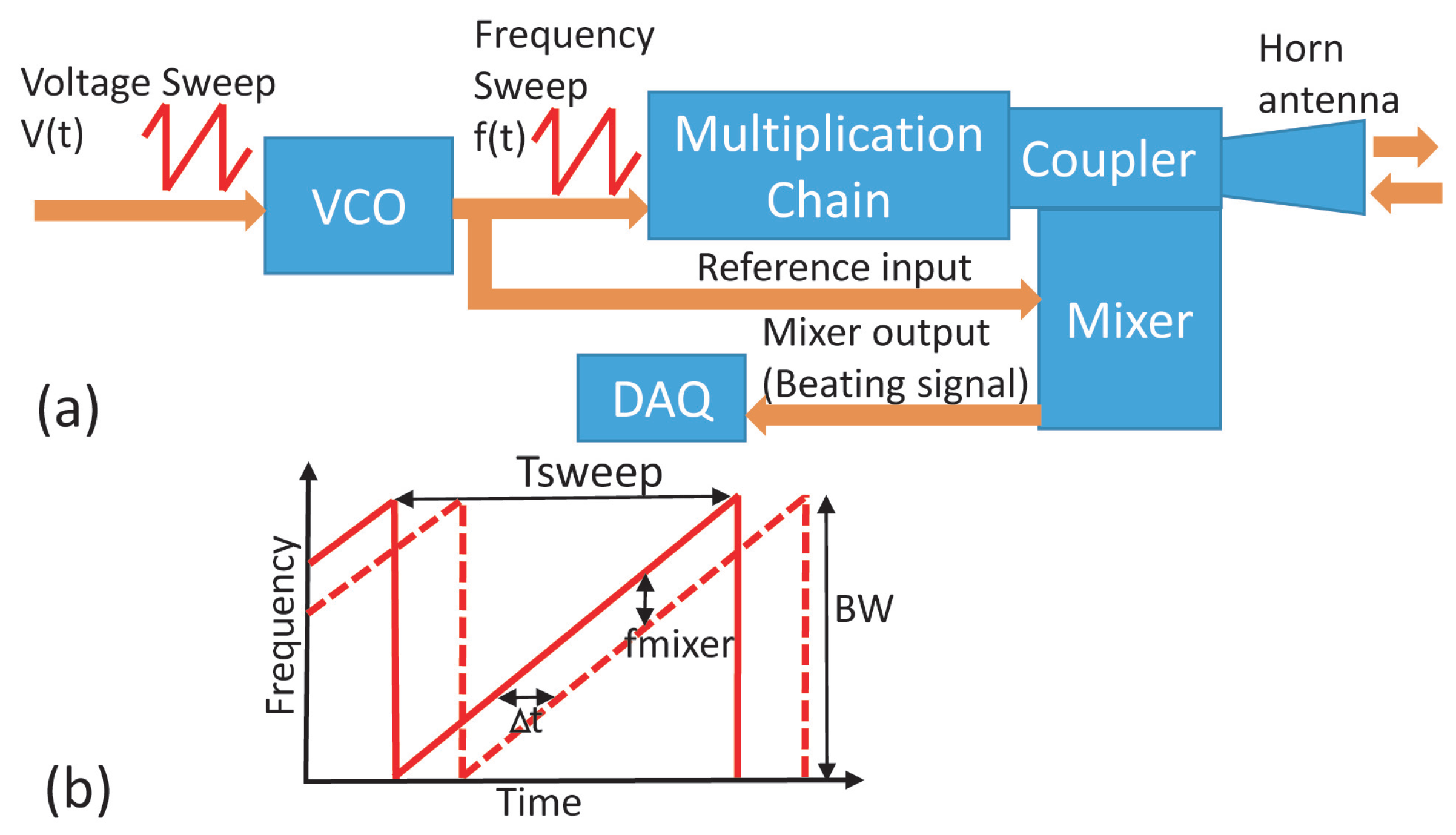
Hence, we propose the use of a 300 GHz FMCW radar to show its feasibility for detecting rock fractures and lithological changes. We present measurements of reservoir rocks, such as dolomite and limestone, and construction rocks, such as granite. The results demonstrated that we could quantify the thicknesses of fractures at the millimeter scale with a centimeter penetration depth, being sensitive to $\mu$fractures and small lithological changes. The acquisition time for imaging a surface of 121 cm${}^2$ with a spatial step of 1 mm and a penetration depth of 3 cm was around 15 min. In addition, we present a method to obtain 3D fracture reconstructions from radar image measurements.

2. Materials and Methods

The experiments were carried out by taking raster scan radar measurements of artificial fractures created by positioning two samples from the same rock with a chosen air gap between them. To test the feasibility of the method for detecting lithological changes, we performed a series of measurements of superposed rocks.

2.1. Samples

Limestone, granite and dolomite samples were taken from different outcrops in the southwest of France. In particular, the limestone samples were partially metamorphosed rocks [22] that formed fracture water reservoirs and the dolomite samples were part of a porous reservoir unit. In addition, the type of limestone and granite samples taken are usually used for construction purposes.

From each rock, two rectangular cubes of different thicknesses were cut out and polished. The chosen thicknesses were greater than the EM wavelength involved to ensure sufficient interactions between the electromagnetic waves and the matter. We also selected thicknesses that provided amplitudes of reflected signals that were detectable by the radar.

The surfaces were ≈ 10 cm × 10 cm and the thicknesses were as follows:

-

Granite ≈ 0.9 cm and ≈ 1.2 cm;

-

Limestone ≈ 1 cm and ≈ 2 cm;

-

Dolomite ≈ 0.5 cm and ≈ 0.8 cm.

The roughness of the rocks was much lower than the EM wavelengths used (≈1 mm) but their thicknesses varied by up to 0.18 cm from point to point. The measurements were made with the use of a caliper, giving an absolute error of 0.02 mm.

2.2. FMCW Radar System

Figure 1a shows the Synview radar architecture used in the measurements [23]. The first stage of the system, working at low frequencies, features a voltage control oscillator (VCO) combined with a phase locked loop (PLL) for stabilization in order to generate fast saw tooth-like frequency sweeps. A multiplier chain is then inserted for the up-conversion to reach the desired working frequency, corresponding to the J band (220 to 330 GHz), with a 275 GHz center frequency. The output power is about 60 $\mathsf{\mu }$W and the dynamic range is 60 dB. The signal is then demodulated and measured with a national instrument data acquisition card. Figure 1b shows the generated chirp signal, with frequency as a function of time. The continuous line represents the emitted signal and the dashed line represents the reflected signal. The distance between the two lines is fixed, which means that the mixer generates an intermediate frequency ($f_{mixer}$), which consists of a tone with a constant frequency. The latter, which is obtained in the frequency domain, is related to the target distance [23]:

$$d=\frac{c_0\Delta t}{2n}=\frac{c_0{f}_{mixer}{T}_{sweep}}{2nBW}$$

(1)

where $c_0$ is the speed of light in a vacuum, $\Delta t$ is the back-and-forth propagation-induced time delay, n is the refracting index of the propagation media at the working frequency, BW is the frequency bandwidth and $T_{sweep}$ is the sweep period.

In the case of multiple reflections, multiple frequency tones are detected. Hence, different distances are measured.

The imaging process can be performed through synthetic aperture radar (SAR) reconstruction or by focusing the radar signal. Both approaches have advantages and disadvantages, depending on the application [24]. Since we aimed for better spatial resolutions, we chose the focusing method. Thus, we used a Teflon lens in the system. Figure 2 shows a schematic of the measurement setup.

In particular, the optical setup included lenses with three focal lengths (50, 100 and 200 mm). We estimated the beam waist diameter (${\omega }_0$) and Rayleigh length ($Z_{Rayleigh}$) for the three cases to select the most suitable option for our application. The Rayleigh length is the distance from the beam waist (in the propagation direction), where the beam radius is increased by a factor of the square root of 2. Assuming a Gaussian beam model of the signal, both parameters could be estimated as follows:

$${\omega }_0=\frac{4\lambda f}{\pi D}$$

(2)

$$Z_{Rayleigh}=\frac{\pi {\omega }_0^2}{\lambda 4}$$

(3)

where f is the lens focal length, D is the signal diameter and $\lambda$ is the wavelength. All of these parameters are depicted in Figure 2. For our application, the best compromise was found using the 100 mm focal length lens as it offered a lateral resolution of 2.5 mm with a Rayleigh length of 4.9 mm, which was close to the size of the fractures that were being studied.

The radar axial resolution is related to the media refractive index and signal bandwidth by

$$\Delta Z=\frac{c_0}{2nBW}$$

(4)

So, given that $BW$ = 90 GHz and n = 1 (in the fracture), the system axial resolution was 1.7 mm. Experimentally, the lateral resolution was confirmed by imaging a USAF target, as described in Figure 3. In the system, the XY stage where the radar was mounted had an accuracy of 0.5 mm.

Before performing a measurement, we calibrated the maximum and minimum amplitude tone frequency signals of the system by reflecting them on metal and without reflecting them, respectively. The metal was placed perpendicular to the signal propagation direction at the focal distance of the Teflon lens (100 mm in our case) to ensure that all reflected signals were collected by the radar. Both measurements established an amplitude scale, which helped to better discriminate noise from reflected signals and set the minimum and maximum of the unit colorbar in the images. Specifically, the latter was presented in dB and the range of colors varied in order to increase the image contrast. This was performed while visualizing the axial images around the fracture or area of interest.

In particular, for each pixel, there is a position given by the motors and a measured signal containing different tones with varying amplitudes in the frequency domain that are proportional to the distances (see Equation (1)). To generate a complete image at a given distance, the amplitudes of the tones located at the same frequency, i.e., the distance of interest, were taken for each motors’ position.

2.3. Measurements

The radar system was set to image a surface of around 11 × 11 cm with a step of 1 mm. Acquired an image took around 15 min. In all measurements, the chosen distance from the Teflon lens to the first rock face was optimized to collect as much as possible the reflected beams. Assuming that the objects were larger than the wavelengths involved and neglecting interference and diffraction, we simulated the system (radar + rocks + artificial fractures) through ray tracing, using the free open-source web application software Ray Optics Simulation. We used the refractive indices of the rocks as presented in the bibliography [25,26]. We found a distance of around 8 cm in all cases. The experiments were rather robust since changing the distance to 7 or 9 cm had no impact on the detected signals.

The first experiments were performed to realize rock fractures by positioning two samples from the same rock parallel to each other with a 5 mm air gap. The thinner samples were put closer to the radar. Figure 4a–c presents the experimental configurations. Then, we measured the limestone samples with variable air gaps (wedged air gaps) to quantify the experimental sensitivity and the axial spatial resolution within the fractures. Figure 4d shows this scenario.

A subsequent series of experiments was carried out with superposed rocks to test the possibility of measuring lithological changes. In Figure 5 are depicted the different studied cases.

3. Results

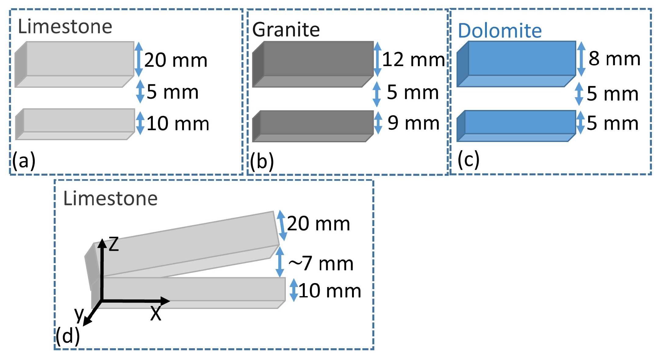
In Figure 6, we present the fracture detection results for the rock configurations shown in Figure 4a–c. For all cases, we show the experimental photographs and the radar images obtained in the axial direction. This means the XY surfaces for different z cuts. Firstly, we present the reflection from the front face of the first rock (named ‘A’), then the reflection from its back face (named ‘B’) and the results obtained when situated in the air gap (named ‘C’). Lastly, we show the reflection from the front face of the second rock (named ‘D’). As previously explained, each pixel in the images represents the tone frequency amplitude detected for the selected distance.

As the thicknesses of the rocks varied and they could be a bit tilted regarding the electromagnetic waves, the images presented for Z-slides did not coincide perfectly with the XY planes of the rocks. Moreover, since the rocks were heterogeneous, e.g., contained fossils, intraclasts and ferromagnesian minerals, the ‘B’ and ‘D’ images did present amplitude variations caused by the EM waves traveling at different velocities ($vel=c_0/n$), and because they underwent different absorption and scattering. However, the two faces of the rocks that mimicked the fracture were identified. It should be noted that when EM waves propagated within a rock, the wavelength was shortened since $\lambda =c_0/\left(n{f}_s\right)$ (where $f_s$ is the signal frequency). Therefore, within the material, the lateral and axial resolutions of the EM signals were smaller in value (see Equations (2) and (4)). This meant that there was an impact on the signal dispersion, depending on the size of the inclusions and fractures.

In the figures, metal marks can be seen. They were metallic tape on the rock that were bigger than the radar lateral resolution to ensure signal reflection. When the electromagnetic signals arrived at the metal, they were fully reflected; thus, a higher amplitude of the frequency tone was measured than that obtained by the variation in the dielectric permittivity of the rock–rock or rock–air interfaces (Fresnell equations). Hence, it helped to identify the rocks’ faces more easily. This is outlined by the red dashed lines.

Especially in the limestone case (Figure 6a), we identified in images ‘A’ and ‘B’ more attenuated regions that corresponded to variations in the thickness of the rock. We signaled this using black dashed lines. Additionally, as expected, in the ‘B’ image, it can be seen that there were more reflected signals where the metallic mark was (and an absence of them in image ‘D’).

In the granite case, the ‘B’ and ‘D’ images presented pixel amplitudes that varied in a grainy way. This could have been caused by the high heterogeneity of the structures. In the photographs, the high quantity of black crystals, e.g., biotites and amphiboles, is visible, which had sizes in the order of the lateral spatial resolution. In image ‘A’, a crack on the surface is visible. This was generated when cutting the sample and only had a depth of a dozen microns.

Lastly, in the dolomite case, in the ’B’ and ’D’ images, it was possible to detect another kind of variation in the pixel amplitudes. They showed a strong preferential direction. In particular, the latter helped us to identify the front face of the second rock due to the high attenuation of the signals.

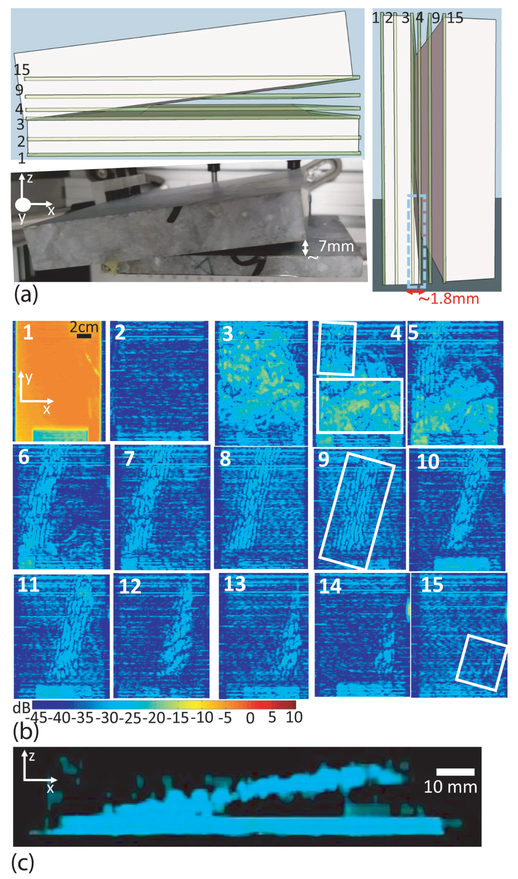
In Figure 7a, we present a photograph and sketches of the experiment shown in Figure 4d. In the drawings, we added in green some axial cuts with the corresponding numbers of radar images presented in Figure 7b. The first radar image shows the first face of the first rock (slide 1). Slide 2 is within the first rock. From slides 3 (the back face of the first rock) to 15, the distance between two consecutive slides is 500 $\mathsf{\mu }$m. In Figure 7a, the blue dashed rectangle signals a thickness variation in the first rock. It was thicker in the bottom part. This is why in slide 4 of Figure 7b we can see in the upper part the reflection from the first face of the second rock, while the reflection in the bottom part was from the second face of the first rock. We indicated this with white solid rectangles. Additionally, in slide 9, we present in the white solid rectangles the reflections from the middle of the first face of the second rock and in slide 15, we present the last reflection obtained. The reflections from the second rock face were inclined with respect to the boundaries (see the white rectangle in slide 9) because the thickness of the first rock increased at the bottom (see the blue rectangle in Figure 7a). Therefore, the reflected signals from the lower part of the second rock face arrived later.

The sequence of images from slide 3 to 15 were utilized to make a 3D reconstruction. We used the open-source image processing software FIJI${}^{TM}$. We first imported the raw images into FIJI and then subtracted any background noise using the subtract background tool. Next, we used the FIJI plug-in ‘3D viewer’ to obtain the 3D image results. We did not interpolate the images. To help with the visualization, the distances used between the slides were 1.4 mm instead of 500 $\mathsf{\mu }$m. Figure 7c presents an upper view of the 3D image. Additionally, we provide a video obtained using the same plug-in, showing an animation of the 3D images, in the Supplementary Materials. In the video, it is possible to notice the variation in the thickness of the first rock. By generating images from different views of the 3D images and using in them the measuring tool from FIJI, it was possible to obtain different parameters for the variation in the thickness and fracture slope of the first rock. We measured a thickness variation of 1.43 mm and in the experiment, it was 1.8 mm. The gap slope (angle between rocks) was obtained using Figure 7c. We obtained 6.5° for the thicker part and we measured $9\pm 2$° in the experiment. In addition, we deduced that the slope in the image appeared clearly when the fracture thickness was around 1.4 mm. This value, as expected, was close to the radar’s axial resolution. However, we could see a gap between the rocks when the distance was around 500 $\mathsf{\mu }$m.

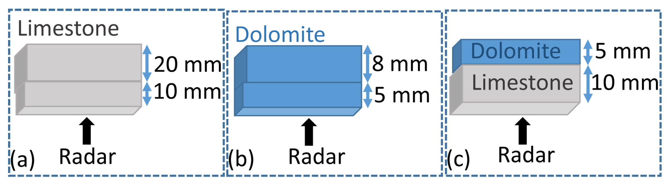
Figure 8 shows the results obtained from the configuration of superposed rocks shown in Figure 5. For each case, we present the radar image from the front face of the first rock, within the first rock and the interface between them. In particular, the front face of the first rock image in Figure 8c shows a color change that we do not see in Figure 8a, which shows the same rock. This indicated that this last rock was tilted with regard to the direction of the electromagnetic signals. Additionally, it should be noted that the rock’s edge in Figure 8b looks irregular. This was related to the rock shape.

In the reported cases, the interfaces were visible. However, we also performed tests by overlaying granite rocks in which the interfaces were not detected.

Although the aim of the study was to detect fractures and lithological changes, we estimated the refractive indices of the rocks to better understand the images and validate the experimental results obtained using the published indices. To do so, we used the distance found between images ‘A’ and ‘B’ in Figure 6a–c and the thicknesses of the rocks ‘H’. In the acquisition program, the distance ‘D’ is estimated by considering that the wave propagates in the air. Therefore, with the obtained ‘$d_A$’ and ‘$d_B$’ values, the refractive indices were estimated using $n=(d_B-d_A)/H$. Thus, $n_{limestone}=2.8$, $n_{dolomite}=2.66$ and $n_{granite}=2.45$. Although these values were approximate since the thicknesses of the samples varied, they are in accordance with the published indices [25,26]. In particular, the refractive index of limestone was closer to that of marble as the samples were partially metamorphosed [22].

The values found showed that the wavelengths were reduced by more than half. If we take a 275 GHz center of frequency for an EM wave propagating in air, we obtain a wavelength of 1 mm, which is reduced to less than 500 $\mathsf{\mu }$m inside a rock. Moreover, as previously mentioned, this also had the impact of more than halving the lateral, as well as the axial, resolution (see Equations (2) and (4)). Therefore, the measurements were even more sensitive to smaller rock heterogeneities. This result also contributed toward explaining the amplitude changes between pixels in the images presented in Figure 6.

We would like to mention that the measurements were carried out and repeated on different days but obtained the same results.

4. Discussion

In this manuscript, we demonstrated that it was possible to clearly detect fractures in rock at a penetration depth of about 1 cm using a 300 GHz radar. However, this depended to a large extent on the dielectric properties of the rocks and their water contents. In particular, the rock samples were not subjected to thermal treatment to evaporate the water contained in their pores and fractures, so the experiments were representative of what is found in nature. Hence, by heating rock samples, a higher penetration could possibly be achieved.

In this work, we did not focus on the heterogeneities or anisotropies of the rocks since this was not the aim of the study. Nevertheless, this information can be seen in the radar images presented in Figure 6b,c. Chiefly, since the granite samples were isotropic, the variations in pixel amplitudes could have been caused by their high mineral heterogeneities. On the other hand, the dolomite samples were more homogeneous but also anisotropic, with higher porosity and water contents. Hence, the radar images might show a preferential direction caused by the water within the pores. In the limestone case, the pixel amplitudes did not vary as much as those in the two other cases. This could have been caused by the fact that limestone is more homogeneous than granite and less porous than dolomite.

Among the results presented in the case of superposed rocks, dolomite looked the least clear. This could have been due to its significant signal absorption behavior, possibly caused by the large amount of water contained in its pores. However, when we conducted the same experiment on granite (which has less absorption), we found no signals coming from the interface. This could have been caused by the fact that the granite is usually isotropic igneous rocks. On the contrary, this is not generally the case with limestone or dolomite, which are sedimentary rocks. This difference could be explained by Figure 8a,b, in which we detected signals from the interface even when the samples were not obtained from the same rock (similar refractive indices). Hence, it could have been mainly caused by the different structure orientations between them, i.e., anisotropy. Note that when superposing the rocks, we did not take into account the orientations of their structures and no air layer was visible between them.

As seen in the results obtained by measuring the wedge air gaps (Figure 7c), the angles found between the rocks were smaller than those measured in the experiments. These results were to be expected considering the effect of the geometry of the reflection of the first face of the second rock, i.e., the electromagnetic waves did not propagate orthogonally with respect to the samples. However, the angles were so small that they did not induce any impact. In the cases where the angles were more than 15 degrees, a formula that relates the dip angles between the reflector and the reflection must be used, as follows (Equation (2.1) in [27]): $RealAngle=arcsin(tan\alpha )$, where $\alpha$ is the angle measured in Figure 7c. Thus, $tan\alpha =Z1/X1$, where Z1 and X1 are the distances measured to calculate the angle. The error was estimated by performing a propagation of uncertainty using the equation $RealAngle=arcsin(Z1/X1)$. The absolute errors of Z1 and X1 were given by the lateral and axial resolutions of the radar system. Therefore, they were responsible for the sensitivity and accuracy of the detected angles. In our case, the estimated error was 2.3°.

The artificial fractures measured in the study contained air. However, in nature, fractures can also contain water or other minerals. In these cases, other approaches, such as that developed in [28], should be applied to obtain information on the dielectric permittivity and thicknesses involved in order to identify the fracture content.

5. Conclusions

In this manuscript, we showed that the use of a 300 GHz FMCW radar allowed for the detection and quantification of millimeter fractures with a sensitivity of up to 500 $\mathsf{\mu }$m at a 1 cm penetration depth in reservoir and construction rocks. Radar images of 121 cm${}^2$ with 1 mm${}^2$ pixels were obtained in 15 min. We also showed that with the acquired images, three-dimensional reconstructions of the fractures could be carried out.

In addition, it was possible to measure lithological changes in two different rock types that were superposed and in two superposed samples from the same rock.

All of these results could be useful for the quality control of construction materials, the characterization of reservoirs, the inspection of buildings or architectural art and even the detection of rock erosion.

Although this method could be used to study any rock material, the results will depend on the absorption, porosity and water content of the constituent minerals, among other factors. Therefore, further studies should be carried out on other reservoir and construction rocks in order to obtain results on a wider range of samples of interest. Additionally, the impacts of rock heterogeneities and anisotropies in high-frequency radar images should be studied as well.

References

1. Hornby, B.E.; Johnson, D.L.; Winkler, K.W.; Plumb, R.A. Fracture evaluation using reflected Stoneley-wave arrivals. Geophysics 1989, 54, 1274–1288. [Google Scholar] [CrossRef]
2. Apel, D.B.; Dezelic, V. Using ground penetrating radar (GPR) in analyzing structural composition of mine roof. Min. Eng. 2005, 57, 56–61. [Google Scholar]
3. Baker, D.R.; Mancini, L.; Polacci, M.; Higgins, M.D.; Gualda, G.A.R.; Hill, R.J.; Rivers, M.L. An introduction to the application of X-ray microtomography to the three-dimensional study of igneous rocks. Lithos 2012, 148, 262–276. [Google Scholar] [CrossRef]
4. Jol, H.M. (Ed.) Ground Penetrating Radar Theory and Applications; Elsevier: Amsterdam, The Netherlands, 2008. [Google Scholar]
5. Lombardi, F.; Podd, F.; Solla, M. From its core to the niche: Insights from GPR applications. Remote Sens. 2022, 14, 3033. [Google Scholar] [CrossRef]
6. Szymczyk, P. Classification of geological structure using Ground-Penetrating Radar and Laplace transform artificial neural networks. Neurocomputing 2015, 148, 354–362. [Google Scholar] [CrossRef]
7. Panoudakis, N.S.; Vafidis, A.; Papavasiliou, A. Delineating a doline system using 3D Ground-Penetrating Radar (GPR) data, complex trace attributes and neural networks: A case study in Omalos Highlands. In Proceedings of the 1st International Conference on Advances in Mineral Resources Management and Environmental Geotechnology, Hania, Greece, 7–9 June 2004. [Google Scholar]
8. Campbell, S.W.; Briggs, M.; Roy, S.G.; Douglas, T.A.; Saari, S. Ground-penetrating radar, electromagnetic induction, terrain, and vegetation observations coupled with machine learning to map permafrost distribution at Twelvemile Lake, Alaska. Permafr. Periglac. Process 2021, 32, 407–426. [Google Scholar] [CrossRef]
9. Qian, Y.; Forghani, M.; Lee, J.H.; Farthing, M.; Hesser, T.; Kitanidis, P.; Darve, E. Application of deep learning-based interpolation methods to nearshore bathymetry. arXiv 2020, arXiv:2011.09707. [Google Scholar]
10. Ball, A.; O’Connor, L. Geologist in the Loop: A Hybrid Intelligence Model for Identifying Geological Boundaries from Augmented Ground-Penetrating Radar. Geosciences 2021, 11, 284. [Google Scholar] [CrossRef]
11. Ivashov, S.I.; Capineri, L.; Bechtel, T.D.; Razevig, V.V.; Inagaki, M.; Gueorguiev, N.L.; Kizilay, A. Design and applications of multi-frequency holographic subsurface radar: Review and case histories. Remote Sens. 2021, 13, 3487. [Google Scholar] [CrossRef]
12. Gutiérrez-Cano, J.D.; Catalá-Civera, J.M.; López-Buendía, A.M.; Plaza-González, P.J.; Penaranda-Foix, F.L. High-Resolution Detection of Rock-Forming Minerals by Permittivity Measurements with a Near-Field Scanning Microwave Microscope. Sensors 2022, 22, 1138. [Google Scholar] [CrossRef]
13. Monti, T.; Tselev, A.; Udoudo, O.; Ivanov, I.N.; Dodds, C.; Kingman, S.W. High-resolution dielectric characterization of minerals: A step towards understanding the basic interactions between microwaves and rocks. Int. J. Miner. Process. 2016, 151, 8–21. [Google Scholar] [CrossRef]
14. Schwerdtfeger, M.; Castro-Camus, E.; Krügener, K.; Viöl, W.; Koch, M. Beating the wavelength limit: Three-dimensional imaging of buried subwavelength fractures in sculpture and construction materials by terahertz time-domain reflection spectroscopy. Appl. Opt. 2013, 52, 375–380. [Google Scholar] [CrossRef] [PubMed]
15. Abina, A.; Puc, U.; Jeglič, A.; Zidanšek, A. Applications of terahertz spectroscopy in the field of construction and building materials. Appl. Spectrosc. Rev. 2015, 50, 279–303. [Google Scholar] [CrossRef]
16. Guntoro, P.I.; Ghorbani, Y.; Koch, P.H.; Rosenkranz, J. X-ray microcomputed tomography (μCT) for mineral characterization: A review of data analysis methods. Minerals 2019, 9, 183. [Google Scholar] [CrossRef]
17. Bassli, A.; Blin, S.; Nouvel, P.; Myara, M.; Roux, J.F.; Benbassou, A.; Belkadid, J.; Pénarier, A. 3-D imaging of materials at 0.1 THz for inner-defect detection using a frequency-modulated continuous-wave radar. IEEE Trans. Instrum. Meas. 2020, 69, 5843–5852. [Google Scholar] [CrossRef]
18. Chopard, A.; Fauquet, F.; Goh, J.S.; Pan, M.; Mounaix, P.; Guillet, J.P.; Simonov, A.; Smolyanskaya, O. Teragogic: Open source platform for low cost millimeter wave sensing and terahertz imaging. In Proceedings of the 2021 IEEE Radar Conference (RadarConf21), Atlanta, GA, USA, 7–14 May 2021; pp. 1–6. [Google Scholar]
19. Dandolo, C.L.K.; Guillet, J.P.; Ma, X.; Fauquet, F.; Roux, M.; Mounaix, P. Terahertz frequency modulated continuous wave imaging advanced data processing for art painting analysis. Opt. Express 2018, 26, 5358–5367. [Google Scholar] [CrossRef]
20. Pan, M.; Chopard, A.; Fauquet, F.; Mounaix, P.; Guillet, J.P. Guided reflectometry imaging unit using millimeter wave FMCW radars. IEEE Trans. Terahertz Sci. Technol. 2020, 10, 647–655. [Google Scholar] [CrossRef]
21. Carré, B.; Chopard, A.; Guillet, J.P.; Fauquet, F.; Mounaix, P.; Gellie, P. Terahertz Nondestructive Testing with Ultra-Wideband FMCW Radar. Sensors 2022, 23, 187. [Google Scholar] [CrossRef]
22. Biteau, J.J.; Marrec, A.L.; Vot, M.L.; Masset, J.M. The aquitaine basin. Pet. Geosci. 2006, 12, 247–273. [Google Scholar] [CrossRef]
23. Chopard, A.; Cassar, Q.; Bou-Sleiman, J.; Guillet, J.P.; Pan, M.; Perraud, J.B.; Susset, A.; Mounaix, P. Terahertz waves for contactless control and imaging in aeronautics industry. NDT Int. 2021, 122, 102473. [Google Scholar] [CrossRef]
24. Cristofani, E.; Friederich, F.; Wohnsiedler, S.; Matheis, C.; Jonuscheit, J.; Vandewal, M.; Beigang, R. Nondestructive testing potential evaluation of a terahertz frequency-modulated continuous-wave imager for composite materials inspection. Opt. Eng. 2014, 53, 031211. [Google Scholar] [CrossRef]
25. Han, D.; Jo, H.; Ahn, J. Terahertz spectroscopy of natural stone materials. In Proceedings of the 2014 39th International Conference on Infrared, Millimeter, and Terahertz waves (IRMMW-THz), Tucson, AZ, USA, 14–19 September 2014; pp. 1–2. [Google Scholar]
26. Zhan, H.; Wu, S.; Zhao, K.; Bao, R.; Xiao, L. CaCO3, its reaction and carbonate rocks: Terahertz spectroscopy investigation. J. Geophys. Eng. 2016, 13, 768–774. [Google Scholar] [CrossRef]
27. Bancroft, J.C. A Practical Understanding of Pre-and Poststack Migrations: Volume 2 (Prestack); Society of Exploration Geophysicists: Tulsa, OK, USA, 2007. [Google Scholar]
28. Tang, W.; Blanche, J.; Mitchell, D.; Harper, S.; Flynn, D. Characterisation of Composite Materials for Wind Turbines Using Frequency Modulated Continuous Wave Sensing. J. Compos. Sci. 2023, 7, 75. [Google Scholar] [CrossRef]
Figure 1. (a) The radar architecture; (b) the chirp signal.
Remotesensing 15 02605 g001
Figure 2. The experimental setup using an FMCW radar.
Remotesensing 15 02605 g002
Figure 3. The USAF target calibration measurement.
Remotesensing 15 02605 g003
Figure 4. The experimental configurations for measuring rock fractures. (a) Limestone case; (b) granite case; (c) dolomite case; (d) Wedge limestone case.
Remotesensing 15 02605 g004
Figure 5. The experimental configurations for measuring lithological changes. (a) Superposed limestones; (b) superposed dolomites; (c) superposed limestone and dolomite.
Remotesensing 15 02605 g005
Figure 6. The experimental photographs and axial images obtained using the configurations presented in Figure 4a–c. (a) Limestone case; (b) granite case; (c) dolomite case.
Remotesensing 15 02605 g006
Figure 7. (a) A photograph and drawings from the experiment presented in Figure 4d; (b) the radar image results; (c) the upper view of the 3D image reconstruction.
Remotesensing 15 02605 g007
Figure 8. The axial images obtained using the configurations presented in Figure 5a–c. (a) Superposed limestones; (b) superposed dolomites; (c) superposed limestone and dolomite.
Remotesensing 15 02605 g008
Disclaimer/Publisher’s Note: The statements, opinions and data contained in all publications are solely those of the individual author(s) and contributor(s) and not of MDPI and/or the editor(s). MDPI and/or the editor(s) disclaim responsibility for any injury to people or property resulting from any ideas, methods, instructions or products referred to in the content.