
Low-Cost Object Detection Models for Traffic Control Devices through Domain Adaption of Geographical Regions
 , ,
, ,  , ,
, ,
Abstract
:1. Introduction
- It provides guidance on the amount of data required for efficient model training to achieve a specific level of accuracy for researchers facing a similar situation to this study (i.e., building a new object detection model, but importing and utilizing data from a model built in another country). This guidance can help prevent unnecessary wastage of resources (time and money) by providing researchers with the appropriate amount of data needed for effective model training, promoting active research activities in the field.
- This study derived multiple condition-specific reference values for the TTCD domain, taking into account different design specifications of the barrel across different nations, use of different pre-trained weights, and different numbers of training datasets. These values can guide researchers in obtaining the appropriate amount of data required for effective model training, further enhancing the accuracy and effectiveness of object detection models in the TTCD domain.
2. Related Studies
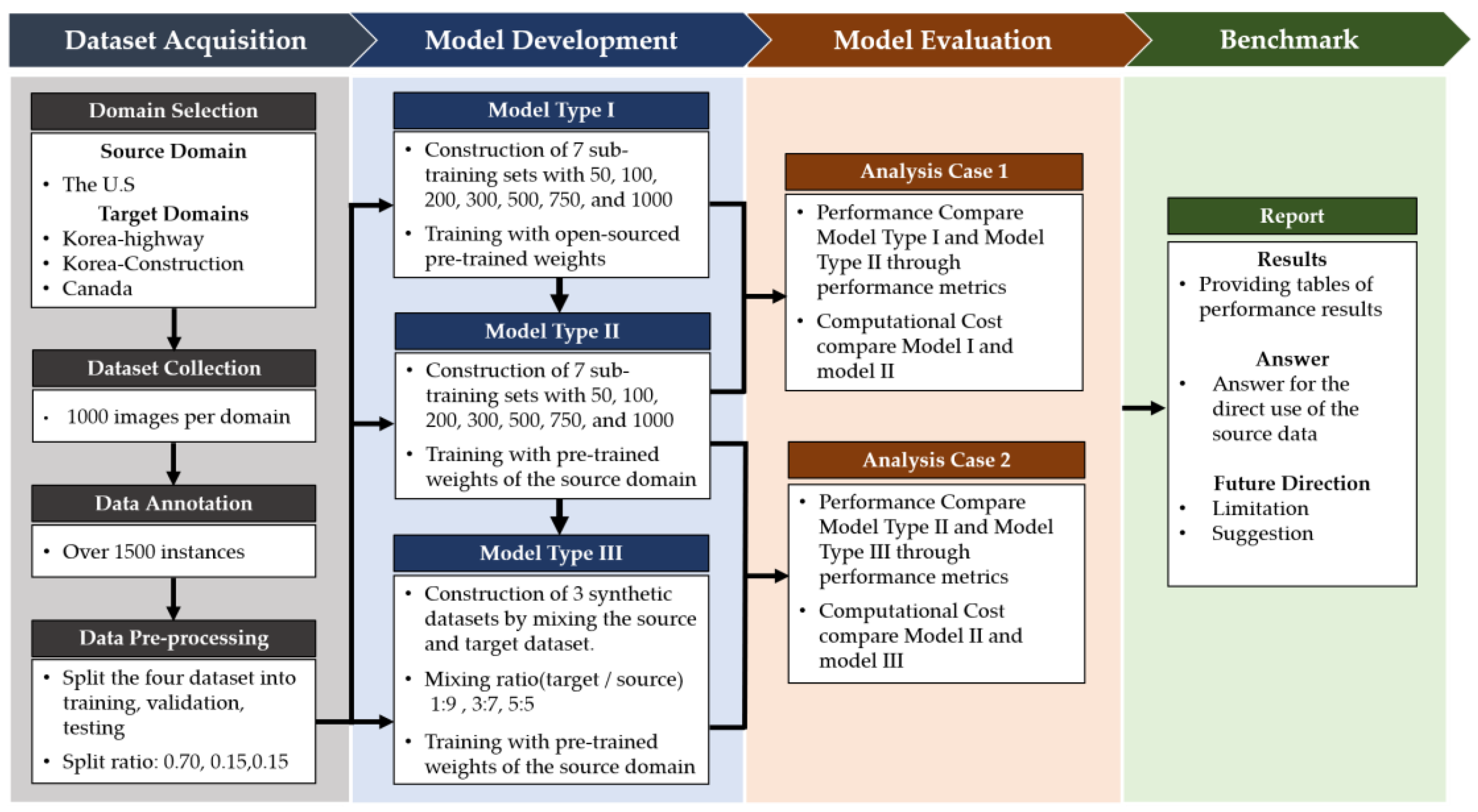
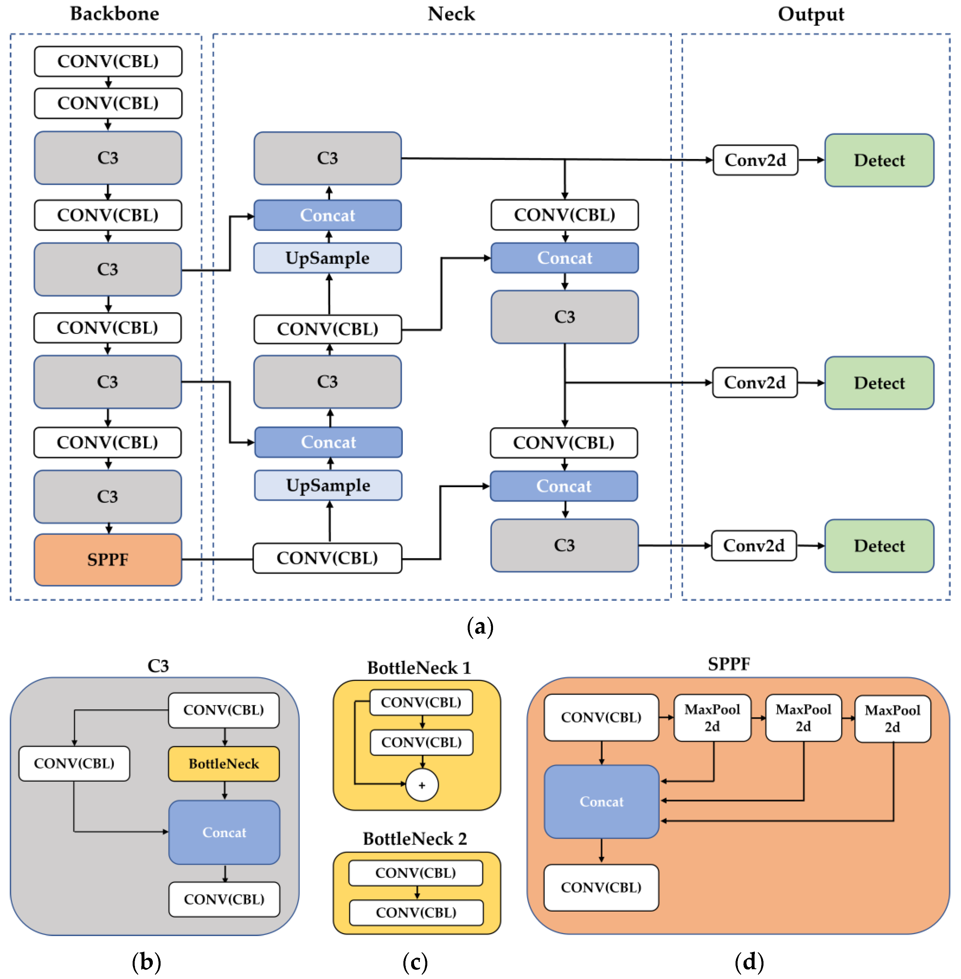
3. Methodology
4. Benchmark
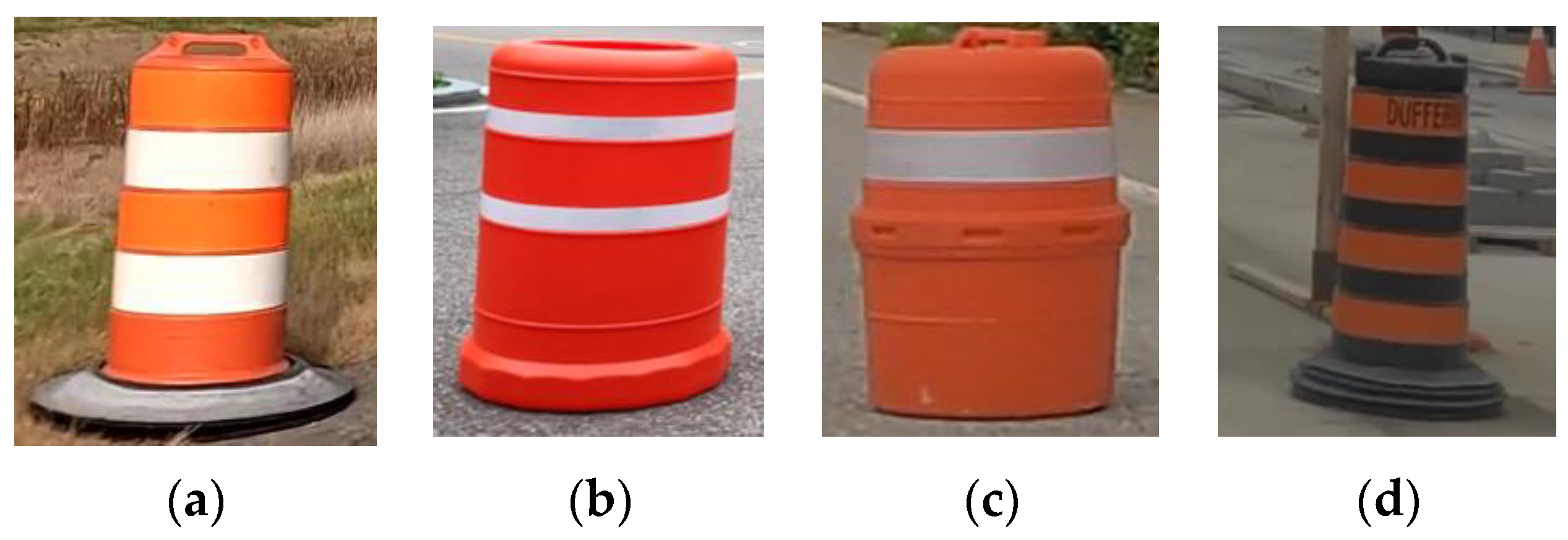
4.1. Dataset Acquisition
4.2. Model Development
4.3. Performance and Cost Evaluation
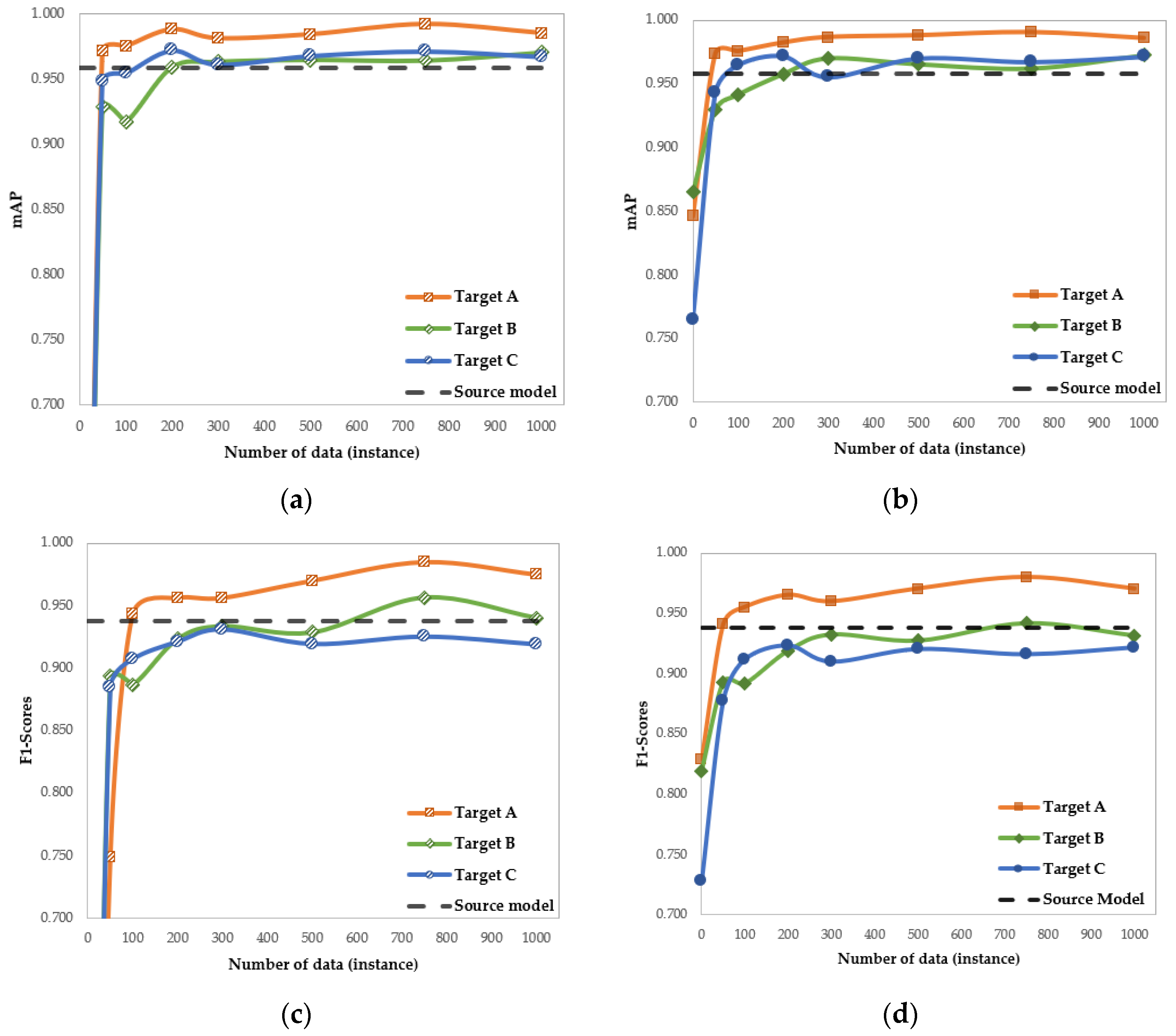
4.3.1. Analysis Case 1—Use of the Pre-Trained Models
4.3.2. Analysis Case 2—Required Target Data
5. Discussion
6. Conclusions
Author Contributions
Funding
Data Availability Statement
Acknowledgments
Conflicts of Interest
References
- Fang, W.; Ding, L.; Zhong, B.; Love, P.; Luo, H. Automated detection of workers and heavy equipment on construction sites: A convolutional neural network approach. Adv. Eng. Inform. 2018, 37, 139–149. [Google Scholar] [CrossRef]
- Delhi, V.; Sankarlal, R.; Thomas, A. Detection of personal protective equipment (PPE) compliance on construction site using computer vision based deep learning techniques. Front. Built. Environ. 2020, 6, 136. [Google Scholar] [CrossRef]
- Chian, E.; Fang, W.; Goh, Y.; Tian, J. Computer vision approaches for detecting missing barricades. Autom. Constr. 2021, 131, 103862. [Google Scholar] [CrossRef]
- Yan, X.; Zhang, H. Computer vision-based disruption management for prefabricated building construction schedule. J. Comput. Civ. Eng. 2021, 35, 04021027. [Google Scholar] [CrossRef]
- Paneru, S.; Jeelani, I. Computer vision applications in construction: Current state, opportunities & challenges. Autom. Constr. 2021, 132, 103940. [Google Scholar] [CrossRef]
- Zaidi, S.; Ansari, M.; Aslam, A.; Kanwal, N.; Asghar, M.; Lee, B. A survey of modern deep learning-based object detection models. Digit. Signal Process. 2022, 126, 103514. [Google Scholar] [CrossRef]
- Li, K.; Wan, G.; Cheng, G.; Meng, L.; Han, J. Object detection in optical remote sensing images: A survey and a new benchmark. ISPRS J. Photogramm. Remote Sens. 2020, 159, 296–307. [Google Scholar] [CrossRef]
- Zhu, X.; Vondrick, C.; Ramanan, D.; Fowlkes, C.C. Do We Need More Training Data or Better Models for Object Detection. BMVC 2012, 3, 11. [Google Scholar]
- Albaranez-Martinez, J.; Llopis-lbor, L.; Hernandez-Garcia, S.; Pineda de Luelmo, S.; Hernandez-Ferrandiz, D. A case of study on traffic cone detection for autonomous racing on a jetson platform. In IbPRIA; Springer: Cham, Switzerland, 2022; pp. 629–641. [Google Scholar] [CrossRef]
- Su, Q.; Wang, H.; Xie, M.; Song, Y.; Ma, S.; Li, B.; Yang, Y.; Wang, L. Real-time traffic cone detection for autonomous driving based on YOLOv4. IET Intell. Transp. Syst. 2022, 16, 1380–1390. [Google Scholar] [CrossRef]
- Zhuang, F.; Qi, Z.; Duan, K.; Xi, D.; Zhu, Y.; Zhu, H.; Xiong, H.; He, Q. A comprehensive survey on transfer learning. Proc. IEEE 2020, 109, 43–76. [Google Scholar] [CrossRef]
- Wang, M.; Deng, W. Deep visual domain adaptation: A survey. Neurocomputing 2018, 312, 135–153. [Google Scholar] [CrossRef]
- Hsu, H.; Yao, C.; Tsai, Y.; Hung, W.; Tseng, H.; Singh, M.; Yang, M. Progressive Domain Adaptation for Object Detection. In Proceedings of the 2020 IEEE Winter Conference on Applications of Computer Vision (WACV), Snowmass, CO, USA, 1–5 March 2020; pp. 738–746. [Google Scholar] [CrossRef]
- Zhao, S.; Yue, X.; Zhang, S.; Li, B.; Zhao, H.; Wu, B.; Krishna, R.; Gonzalez, J.E.; Sangiovanni-Vincentelli, A.L.; Seshia, S.A.; et al. A review of single-source deep unsupervised visual domain adaptation. IEEE Trans. Neural Netw. Learn. Syst. 2020, 33, 473–493. [Google Scholar] [CrossRef]
- Tseng, H.; Lee, H.; Huang, J.; Yang, M. Cross-domain few-shot classification via learned feature-wise transformation. arXiv 2020, arXiv:2001.08735. [Google Scholar] [CrossRef]
- Kim, Y.; Cho, D.; Han, K.; Panda, P.; Hong, S. Domain adaptation without source data. IEEE TAI 2021, 2, 508–518. [Google Scholar] [CrossRef]
- Na, S.; Heo, S.; Han, S.; Shin, Y.; Lee, M. Development of an artificial intelligence model to recognize construction waste by applying image data augmentation and transfer learning. Buildings 2022, 12, 175. [Google Scholar] [CrossRef]
- Wang, Z.; Yang, J.; Jiang, H.; Fan, X. CNN training with twenty samples for crack detection via data augmentation. Sensors 2020, 20, 4849. [Google Scholar] [CrossRef] [PubMed]
- Chen, Y.; Liu, Q.; Wang, T.; Wang, B.; Meng, X. Rotation-Invariant and Relation-Aware Cross-Domain Adaptation Object Detection Network for Optical Remote Sensing Images. Remote Sens. 2021, 13, 4386. [Google Scholar] [CrossRef]
- Stallkamp, J.; Schlipsing, M.; Salmen, J.; Igel, C. The German Traffic Sign Recognition Benchmark: A multi-class classification competition. In Proceedings of the 2011 International Joint Conference on Neural Networks, San Jose, CA, USA, 31 July–5 August 2011; pp. 1453–1460. [Google Scholar] [CrossRef]
- Timofte, R.; Zimmermann, K.; Van Gool, L. Multi-view traffic sign detection, recognition, and 3D localisation. Mach. Vis. Appl. 2014, 25, 633–647. [Google Scholar] [CrossRef]
- Larsson, F.; Felsberg, M. Using Fourier Descriptors and Spatial Models for Traffic Sign Recognition. In Image Analysis SCIA, 2nd ed.; Heyden, A., Kahl, F., Eds.; Springer: Berlin/Heidelberg, Germany, 2011; Volume 6688, pp. 238–249. [Google Scholar] [CrossRef]
- Mogelmose, A.; Trivedi, M.; Moeslund, T. Vision-based traffic sign detection and analysis for intelligent driver assistance systems: Perspectives and survey. IEEE T-ITS 2012, 13, 1484–1497. [Google Scholar] [CrossRef]
- Zhu, Z.; Liang, D.; Zhang, S.; Huang, X.; Li, B.; Hu, S. Traffic-Sign Detection and Classification in the Wild. In Proceedings of the IEEE Conference on Computer Vision and Pattern Recognition, Las Vegas, NV, USA, 27–30 June 2016; pp. 2110–2118. [Google Scholar] [CrossRef]
- Dhall, A.; Dai, D.; Van Gool, L. Real-time 3D Traffic Cone Detection for Autonomous Driving. In Proceedings of the 2019 IEEE Intelligent Vehicles Symposium (IV), Paris, France, 9–12 June 2019; pp. 494–501. [Google Scholar] [CrossRef]
- Katsamenis, I.; Karolou, E.E.; Davradou, A.; Protopapadakis, E.; Doulamis, A.; Doulamis, N.; Kalogeras, D. TraCon: A Novel Dataset for Real-Time Traffic Cones Detection Using Deep Learning. In NiDS, 2nd ed.; Krouska, A., Troussas, C., Caro, J., Eds.; Springer: Cham, Switzerland, 2022; Volume 556, pp. 382–391. [Google Scholar] [CrossRef]
- Kang, K.; Chen, D.; Peng, C.; Koo, D.; Kang, T.; Kim, J. Development of an automated visibility analysis framework for pavement markings based on the deep learning approach. Remote Sens. 2020, 12, 3837. [Google Scholar] [CrossRef]
- Kim, Y.; Song, K.; Kang, K. Framework for Machine Learning-Based Pavement Marking Inspection and Geohash-Based Monitoring; ICTD: Seattle, WA, USA, 2022; pp. 123–132. [Google Scholar] [CrossRef]
- Seo, S.; Chen, D.; Kim, K.; Kang, K.; Koo, D.; Chae, M.; Park, H. Temporary traffic control device detection for road construction projects using deep learning application. Constr. Res. Congr. 2022, 392–401. [Google Scholar]
- Song, K.; Chen, D.; Seo, S.; Jeon, J.; Kang, K. Feasibility of Deep Learning in Segmentation of Road Construction Work Zone Using Vehicle-Mounted Monocular Camera; UKC: Chicago, IL, USA, 2021; pp. 15–18. [Google Scholar]
- Csurka, G. Domain adaptation for visual applications: A comprehensive survey. arXiv 2017, arXiv:1702.05374. [Google Scholar]
- Yosinski, J.; Clune, J.; Bengio, Y.; Lipson, H. How transferable are features in deep neural networks? arXiv 2014, arXiv:1411.1792. [Google Scholar]
- Shahinfar, S.; Meek, P.; Falzon, G. How many images do I need? Understanding how sample size per class affects deep learning model performance metrics for balanced designs in autonomous wildlife monitoring. Ecol. Inform. 2020, 57, 101085. [Google Scholar] [CrossRef]
- Sharma, T.; Debaque, B.; Duclos, N.; Chehri, A.; Kinder, B.; Fortier, P. Deep Learning-Based Object Detection and Scene Perception under Bad Weather Conditions. Electronics 2022, 11, 563. [Google Scholar] [CrossRef]
- Guo, Y.; Shi, H.; Kumar, H.; Grauman, K.; Rosing, T.; Feris, R. SpotTune: Transfer Learning Through Adaptive Fine-Tuning. In Proceedings of the 2019 IEEE/CVF Conference on Computer Vision and Pattern Recognition (CVPR), Long Beach, CA, USA, 15–20 June 2019; pp. 4800–4809. [Google Scholar] [CrossRef]
- Misra, I.; Shrivastava, A.; Gupta, A.; Hebert, M. Cross-Stitch Networks for Multi-task Learning. In Proceedings of the 2016 IEEE Conference on Computer Vision and Pattern Recognition (CVPR), Las Vegas, NV, USA, 27–30 June 2016; pp. 3994–4003. [Google Scholar] [CrossRef]
- Bengio, Y. Deep learning of representations for unsupervised and transfer learning. In Proceedings of the ICML Workshop on Unsupervised and Transfer Learning. JMLR Workshop and Conference Proceedings, Washington, DC, USA, 2 July 2011; pp. 17–36. [Google Scholar]
- Bruzzone, L.; Marconcini, M. Domain adaptation problems: A dasvm classification technique and a circular validation strategy. IEEE TPAMI 2010, 32, 770–787. [Google Scholar] [CrossRef] [PubMed]
- Chu, W.S.; De la Torre, F.; Cohn, J.F. Selective transfer machine for personalized facial action unit detection. In Proceedings of the IEEE Conference on Computer Vision and Pattern Recognition, Portland, OR, USA, 23–28 June 2013; pp. 3515–3522. [Google Scholar]
- Gong, B.; Grauman, K.; Sha, F. Connecting the dots with landmarks: Discriminatively learning domain-invariant features for unsupervised domain adaptation. PMLR 2013, 28, 222–230. [Google Scholar]
- Pan, S.J.; Yang, Q. A survey on transfer learning. IEEE Trans. Knowl. Data Eng. 2010, 22, 1345–1359. [Google Scholar] [CrossRef]
- Goodfellow, I.; Pouget-Abadie, J.; Mirza, M.; Xu, B.; Warde-Farley, D.; Ozair, S.; Courville, A.; Bengio, Y. Generative adversarial nets. NIPS 2014, 63, 2672–2680. [Google Scholar] [CrossRef]
- Xu, W.; He, J.; Shu, Y. Transfer learning and deep domain adaptation. Adv. Appl. Deep Learn. 2020, 45. [Google Scholar] [CrossRef]
- Rostami, M.; Kolouri, S.; Eaton, E.; Kim, K. Deep transfer learning for few-shot SAR image classification. Remote Sens. 2019, 11, 1374. [Google Scholar] [CrossRef]
- Wang, W.; Ma, L.; Chen, M.; Du, Q. Joint correlation alignment-based graph neural network for domain adaptation of multitemporal hyperspectral remote sensing images. IEEE J-STARS 2021, 14, 3170–3184. [Google Scholar] [CrossRef]
- Lasloum, T.; Alhichri, H.; Bazi, Y.; Alajlan, N. SSDAN: Multi-source semi-supervised domain adaptation network for remote sensing scene classification. Remote Sens. 2021, 13, 3861. [Google Scholar] [CrossRef]
- Zheng, Z.; Zhong, Y.; Su, Y.; Ma, A. Domain adaptation via a task-specific classifier framework for remote sensing cross-scene classification. IEEE Trans Geosci. Remote Sens. 2022, 60, 4416212. [Google Scholar] [CrossRef]
- Federal Highway Administration (FHWA). Manual on Uniform Traffic Control Devices (MUTCD); FHWA: Washington, DC, USA, 2009.
- Ministry of Land, Infrastructure and Transportation (MOLIT). Traffic Management Guidelines for Road 25 Construction Sites; MOLIT: Sejong, Republic of Korea, 2018.
- Ontario Traffic Manual (OTM). Book 7: Temporary Conditions; Ontario Ministry of Transportation: St. Catherines, ON, Canada, 2014.
- Jocher, G.; Chaurasia, A.; Stoken, A.; Borovec, J.; Kwon, Y.; Michael, K. ultralytics/yolov5: v7. 0-YOLOv5 SOTA Realtime Instance Segmentation; 2022. Zenodo. Available online: https://zenodo.org/record/7347926#.ZGHTqXxByUk (accessed on 16 April 2023).
- Wang, J.; Chen, Y.; Dong, Z.; Gao, M. Improved YOLOv5 network for real-time multi-scale traffic sign detection. Neural Comput. Appl. 2022, 35, 7853–7865. [Google Scholar] [CrossRef]
- Zhu, Y.; Yan, W.Q. Traffic sign recognition based on deep learning. Multimed. Tools Appl. 2022, 81, 17779–17791. [Google Scholar] [CrossRef]
- He, K.; Zhang, X.; Ren, S.; Sun, J. Spatial Pyramid Pooling in Deep Convolutional Networks for Visual Recognition. IEEE TPAMI 2015, 37, 1904–1916. [Google Scholar] [CrossRef]
- Golubeva, A.; Neyshabur, B.; Gur-Ari, G. Are wider nets better given the same number of parameters? arXiv 2020, arXiv:2010.14495. [Google Scholar]
- Liu, Y.; He, G.; Wang, Z.; Li, W.; Huang, H. NRT-YOLO: Improved YOLOv5 Based on Nested Residual Transformer for Tiny Remote Sensing Object Detection. Sensors 2022, 22, 4953. [Google Scholar] [CrossRef]
- Zheng, Z.; Wang, P.; Liu, W.; Li, J.; Ye, R.; Ren, D. Distance-IoU Loss: Faster and Better Learning for Bounding Box Regression. In Proceedings of the 2020 AAAI Conference on Artificial Intelligence, New York, NY, USA, 7–12 February 2020; pp. 12993–13000. [Google Scholar] [CrossRef]
- Lin, T.Y.; Maire, M.; Belongie, S.; Hays, J.; Perona, P.; Ramanan, D.; Dollár, P.; Zitnick, C.L. Microsoft COCO: Common Objects in Context. In Lecture Notes in Computer Science, 2nd ed.; Fleet, D., Pajdla, T., Schiele, B., Tuytelaars, T., Eds.; Springer: Cham, Switzerland, 2014; Volume 8693. [Google Scholar] [CrossRef]
- Padilla, R.; Passos, W.L.; Dias, T.L.B.; Netto, S.L.; da Silva, E.A. A Survey on Performance Metrics for Object-Detection Algorithms. In Proceedings of the 2020 International Conference on Systems, Signals and Image Processing (IWSSIP), Niteroi, Brazil, 1–3 July 2020; pp. 237–242. [Google Scholar] [CrossRef]
- Zhang, X.; Wang, W.; Zhao, Y.; Xie, H. An improved YOLOv3 model based on skipping connections and spatial pyramid pooling. Syst. Sci. Control Eng. 2021, 9, 142–149. [Google Scholar] [CrossRef]
- Padilla, R.; Passos, W.L.; Dias, T.L.B.; Netto, S.L.; da Silva, E.A.B. A Comparative Analysis of Object Detection Metrics with a Companion Open-Source Toolkit. Electronics 2021, 10, 279. [Google Scholar] [CrossRef]
- Brechner, R.; Bergeman, G. Contemporary Mathematics for Business & Consumers, 8th ed.; Cengage Learning: Boston, MA, USA, 2016. [Google Scholar]
- Tajbakhsh, N.N.; Shin, J.; Gurudu, S.; Hurst, R.; Kendall, C.; Gotway, M.; Liang, J. Convolutional Neural Networks for Medical Image Analysis: Full Training or Fine Tuning? IEEE Trans. Med. Imaging 2016, 35, 1299–1312. [Google Scholar] [CrossRef]
- Smith, L.N. A disciplined approach to neural network hyper-parameters: Part 1—Learning rate, batch size, momentum, and weight decay. arXiv 2018, arXiv:1803.09820. [Google Scholar]
- Isa, I.S.; Rosli, M.S.A.; Yusof, U.K.; Maruzuki, M.I.F.; Sulaiman, S.N. Optimizing the Hyperparameter Tuning of YOLOv5 for Underwater Detection. IEEE Access 2022, 10, 52818–52831. [Google Scholar] [CrossRef]
- Gayakwad, E.; Prabhu, J.; Anand, R.V.; Kumar, M.S. Training Time Reduction in Transfer Learning for a Similar Dataset Using Deep Learning. In Intelligent Data Engineering and Analytics, 2nd ed.; Satapathy, S., Zhang, Y.D., Bhateja, V., Majhi, R., Eds.; Springer: Cham, Switzerland, 2021; Volume 1177, pp. 359–367. [Google Scholar] [CrossRef]
- Xu, Y.; Zhong, X.; Yepes, A.J.J.; Lau, J.H. Forget me not: Reducing catastrophic forgetting for domain adaptation in reading comprehension. In Proceedings of the 2020 International Joint Conference on Neural Networks (IJCNN), Glasgow, UK, 19–24 July 2020; pp. 1–8. [Google Scholar] [CrossRef]
- Sun, C.; Shrivastava, A.; Singh, S.; Gupta, A. Revisiting Unreasonable Effectiveness of Data in Deep Learning Era. In Proceedings of the IEEE International Conference on Computer Vision, Venice, Italy, 22–29 October 2017; pp. 843–852. [Google Scholar] [CrossRef]
- Tabak, M.A.; Norouzzadeh, M.S.; Wolfson, D.W.; Sweeney, S.J.; VerCauteren, K.C.; Snow, N.P.; Halseth, J.M.; Di Salvo, P.A.; Lewis, J.S.; White, M.D.; et al. Machine learning to classify animal species in camera trap images: Applications in ecology. Methods Ecol. Evol. 2019, 10, 585–590. [Google Scholar] [CrossRef]
- Korea Ministry of Science and ICT. National Strategy for Artificial Intelligence; MIST: Sejong-Si, Republic of Korea, 2019.


| Types | Model I | Model II | Model III | |
|---|---|---|---|---|
| Training Dataset | Only Target | Only Target | Mix (Source + Target) | |
| # Number of Training Sets (# Number of Instance) | 7 (50, 100, 200, 300, 500, 750, and 1000) | 7 (50, 100, 200, 300, 500, 750, and 1000) | 3 mixing ratios (1:9, 3:7, and 5:5) | |
| Pre-Trained Model | YOLOv5L using COCO | Source Model | Source Model | |
| Target | A (Korean Barrel for Highway) | 7 | 7 | 3 |
| B (Korean barrel for short-term construction) | 7 | 7 | 3 | |
| C (Canada Barrel) | 7 | 7 | 3 | |
| Total constructed model | 28 | 28 | 12 | |
| Testing Set | Precision | Recall | F1 Score | mAP_0.5 1 |
|---|---|---|---|---|
| Source S | 0.923 | 0.953 | 0.938 | 0.958 |
| Target A | 0.905 | 0.765 | 0.829 | 0.846 |
| Target B | 0.848 | 0.792 | 0.819 | 0.865 |
| Target C | 0.885 | 0.618 | 0.728 | 0.765 |
| Percentage Variance (%) 2 | |||
|---|---|---|---|
| Labeled Instances | Target A | Target B | Target C |
| 50 | −8.7% | −17.1% | −5.6% |
| 100 | −27.7% | −97.5% | +0.1% |
| 200 | −2.7% | −0.8% | −42.1% |
| 300 | +1.4% | −0.2% | +1.7% |
| 500 | −0.2% | +0.6% | −1.7% |
| 1000 | −57.9% | −156.6% | −98.7% |
| Percentage Variance (%) 3 | |||
|---|---|---|---|
| Labeled Instances | Target A | Target B | Target C |
| (1:9) 100:900 | 495% | 1560% | 849% |
| (3:7) 300:700 | 230% | 241% | 314% |
| (5:5) 500:500 | 17% | 138% | 253% |
| Model Type | Number of Trained Data | mAP_0.5 | % mAP Variance | ||||
|---|---|---|---|---|---|---|---|
| Target A | Target B | Target C | Target A | Target B | Target C | ||
| Type II | 100 | 0.930 | 0.950 | 0.911 | −3% | −1% | −5% |
| 300 | 0.841 | 0.900 | 0.872 | −14% | −6% | −10% | |
| 500 | 0.723 | 0.861 | 0.861 | −33% | −11% | −11% | |
| Type III | (1:9) 100 | 0.954 | 0.963 | 0.961 | 0% | 1% | 0% |
| (3:7) 300 | 0.958 | 0.952 | 0.941 | 0% | −1% | −2% | |
| (5:5) 500 | 0.953 | 0.948 | 0.951 | −1% | −1% | −1% | |
Disclaimer/Publisher’s Note: The statements, opinions and data contained in all publications are solely those of the individual author(s) and contributor(s) and not of MDPI and/or the editor(s). MDPI and/or the editor(s) disclaim responsibility for any injury to people or property resulting from any ideas, methods, instructions or products referred to in the content. |
© 2023 by the authors. Licensee MDPI, Basel, Switzerland. This article is an open access article distributed under the terms and conditions of the Creative Commons Attribution (CC BY) license (https://creativecommons.org/licenses/by/4.0/).
Share and Cite
Oh, D.; Kang, K.; Seo, S.; Xiao, J.; Jang, K.; Kim, K.; Park, H.; Won, J. Low-Cost Object Detection Models for Traffic Control Devices through Domain Adaption of Geographical Regions. Remote Sens. 2023, 15, 2584. https://doi.org/10.3390/rs15102584
Oh D, Kang K, Seo S, Xiao J, Jang K, Kim K, Park H, Won J. Low-Cost Object Detection Models for Traffic Control Devices through Domain Adaption of Geographical Regions. Remote Sensing. 2023; 15(10):2584. https://doi.org/10.3390/rs15102584
Chicago/Turabian StyleOh, Dahyun, Kyubyung Kang, Sungchul Seo, Jinwu Xiao, Kyochul Jang, Kibum Kim, Hyungkeun Park, and Jeonghun Won. 2023. "Low-Cost Object Detection Models for Traffic Control Devices through Domain Adaption of Geographical Regions" Remote Sensing 15, no. 10: 2584. https://doi.org/10.3390/rs15102584