Satellite-Derived Bathymetry Mapping on Horseshoe Island, Antarctic Peninsula, with Open-Source Satellite Images: Evaluation of Atmospheric Correction Methods and Empirical Models

Abstract

Satellite-derived bathymetry (SDB) is the process of estimating water depth in shallow coastal and inland waters using satellite imagery. Recent advances in technology and data processing have led to improvements in the accuracy and availability of SDB. The increased availability of free optical satellite sensors, such as Landsat missions and Sentinel 2 satellites, has increased the quantity and frequency of SDB research and mapping efforts. In addition, machine learning (ML)- and deep learning (DL)-based algorithms, which can learn to identify features that are indicative of water depth, such as color or texture variations, have started to be used for extracting bathymetry information from satellite imagery. This study aims to produce an initial optical image-based SBD map of Horseshoe Island’s shallow coasts and to perform a comprehensive and comparative evaluation with Landsat 8 and Sentinel 2 satellite images. Our research considers the performance of empirical SDB models (classical, ML-based, and DL-based) and the effects of the atmospheric correction methods ACOLITE, iCOR, and ATCOR. For all band combinations and depth intervals, the ML-based random forest and XGBoost models delivered the highest performance and best fitting ability by achieving the lowest error with MAEs smaller than 1 m up to 10 m depth and a maximum correlation of R² around 0.80. These models are followed by the DL-based ANN and CNN models. Nonetheless, the non-linearity of the reflectance–depth connection was significantly reduced by the ML-based models. Furthermore, Landsat 8 showed better performance for 10–20 m depth intervals and in the entire range of (0–20 m), while Sentinel 2 was slightly better up to 10 m depth intervals. Lastly, ACOLITE, iCOR, and ATCOR provided reliable and consistent results for SDB, where ACOLITE provided the highest automation.

1. Introduction

Shallow water bathymetry is crucial for nautical navigation, but it is also essential for monitoring coastal areas covering underwater topography, sediment loads, detection and identification of human-induced pressures, and the effects of changes in the climate such as sea level rise [1,2]. The adverse effects of climate change have been more evident in the last and hottest decade resulting in massive heatwaves and temperature rise, especially in polar regions. Several studies have pointed out that the Antarctic Peninsula and sub-Antarctic islands have faced rapid warming with the highest temperature records and acceleration in snowbank melting [3,4,5]. Thus, there is a need for continuous monitoring of the ecosystem and sea level rise in shallow zones.

The conventional approaches for surveying seas and oceans use single (SBE) and multi-beam echosounders (MBEs). Yet these methods bear certain limitations, such as losing their efficacy as depth decreases, having a limited spatial coverage and temporal resolution, and being subject to logistic restrictions with high operational costs and risks [1]. Recently, a range of modern tools have been used to assess the ocean’s bathymetry, including remotely operated vehicles, automated underwater vehicles, and airborne LIDAR platforms [6]. However, according to the study of Ashphaq et al., remote and autonomous technologies are likewise expensive due to costs associated with their purchase and maintenance [7].

Due to their capacity to collect data across vast spatial areas and to offer high-frequency temporal monitoring, space-borne remote sensing techniques have additionally been developed into a substitute method for obtaining bathymetric data in coastal zones [8]. The method developed to survey shallow waters with optical satellite images is called satellite-derived bathymetry (SDB). Optical SDB is based on the inverse relationship between the amount of energy reflected from the water column and the depth of water [1]. As stated by Duan et al., recent studies have focused on SDB technology within the scope of producing bathymetry data [9]. Remote sensing data eliminate traditional bathymetric surveying because of their low cost, broad regional coverage, and temporal and space-unconstrained sensing abilities [10]. It is clear that SDB research is rising, as shown in the sharp increase over the past five years according to a literature review in the Web of Science collection using the keywords “satellite”, “remote sensing”, “bathymetry”, etc. Especially, Landsat 8 and Sentinel 2 open-source optical satellites have shown expanded research capability on the optical SDB field and provide high potential in bathymetry estimation of coastal and inland regions [9,11,12,13].

It can be stated that initial studies based on linear and logarithmic band ratio-based algorithms [14,15] were followed by machine learning (ML) algorithms and DL-based approaches that are nowadays available based on a chronological review of empirical SDB studies. The initial use of ML-based SDB mapping was introduced by Ceyhun and Yalcın [16], and the popular use of ML-based approaches was observed coupled with the support vector machine (SVM) algorithm [9,17], followed by the random forest (RF) [9,18,19,20] and XGBoost algorithms [21,22]. Among them, the use of XGBoost in optical SDB is relatively new, and only two studies have been undertaken to infer bathymetric depth from Sentinel 2 satellite images. Susa’s study, drawing attention to the current use of XGBoost, suggested further investigation of its performance [22]. The DL-based SDB mapping is a recent research attempt, which mainly focuses on determining the local spatial correlation between the reflectance information and the water depth. Initial studies used artificial neural networks (ANNs) for SDB mapping and reported considerable improvements in accuracy with respect to classical models [23,24]. Another study by Dickens and Armstrong used recurrent neural networks (RNNs) on Orbview 3 satellite images to derive SDB in Pacific islands [25]. A more recent study used convolutional neural networks (CNNs) to identify the relationship and produce SDB maps at spatial resolutions compatible with multispectral images [26]. Recently, Wan and Ma used a deep belief network with a data perturbation (DBN-DP) model on Quickbird and Worldview 2 images in which R² correlation and RMSE metrics in comparison with other models used in the study were reported [27]. A recent study published in 2023 compared basic empirical models and ML-based methods (RF, SVM, and NN) in SDB mapping of the Ganquan Dao area and their findings provided higher inversion results with ML-based methods in up to 15 m depth. The authors of the study pointed out that a comparative analysis of empirical and ML-based methods in different water depths is still scarce and inconclusive [28].

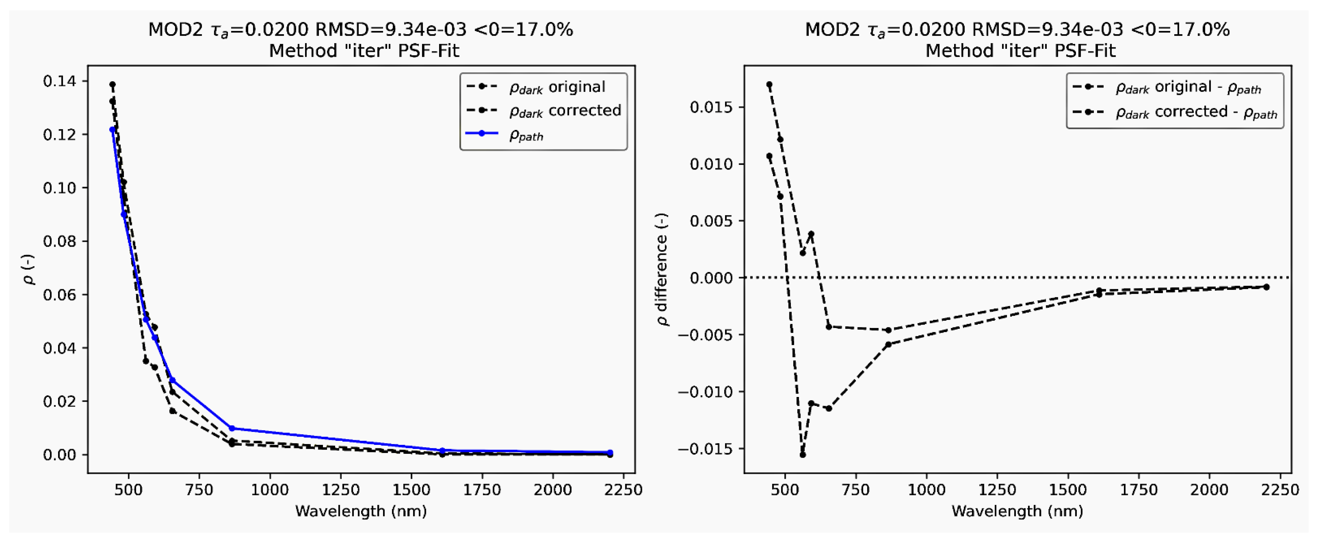
The atmospheric correction process is frequently addressed as a crucial step when satellite images are used for bathymetry extraction [29,30]. The complexity of the water column in coastal waters caused by factors such as water quality and sediment heterogeneity has an impact on the proper measurement of water depth. This situation suggests a stricter requirement for atmospheric correction accuracy [12]. Several recent studies have experimentally compared the performance of various atmospheric correction algorithms and examined the comparative correlation between ground-based depth measurements and/or image band ratios and estimated depth [30,31]. Among these studies, Caballero and Stumpf showed that the performance of atmospheric correction directly affects empirical methods based on band ratio [30]. Ceyhun and Yalcin stated that machine learning-based approaches in particular do not consider the behavioral mechanism of electromagnetic radiation in water; therefore, the effect of atmospheric correction is minimal [16]. On the other hand, Duan et al. obtained significant correlation differences depending on the atmospheric correction model on the machine learning-based SVM algorithm, and they stated that there is still a need for a systematic comparison of the effects of different atmospheric correction algorithms on different SDB models [9].

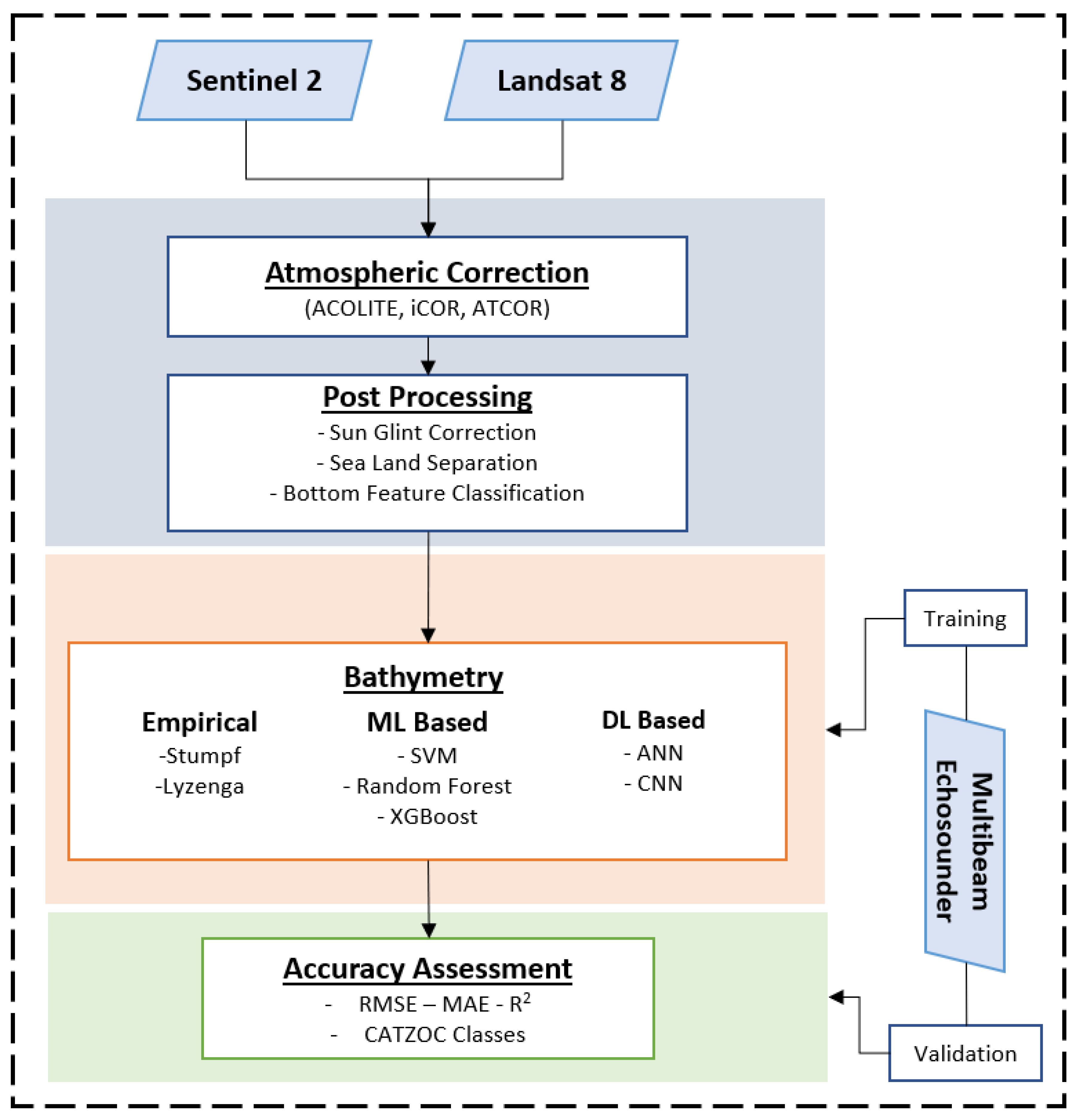
This study focuses on estimating and mapping the bathymetry on Horseshoe Island, Antarctic Peninsula, by performing a comprehensive evaluation of atmospheric correction effects on SDB with Landsat 8 and Sentinel 2 images, and by comparing the performance of ML- and DL-based models with the basic empirical models. To the best of our knowledge, this study is one of the first studies to conduct a thorough evaluation of SDB mapping with optical satellite images in Antarctica, considering sensor platforms, atmospheric correction methods, and empirical SBD models.

The main contributions of this study to the literature are the following:

• Demonstration of a comparative performance evaluation of empirical SDB mapping approaches with an extension of the most current ML- and DL-based methods in Antarctica.
• Evaluation of the effects of the state-of-the-art atmospheric correction methods on SDB mapping for a region with complex and challenging atmospheric conditions such as Antarctica.
• Investigation of the suitability of open source mid-resolution optical satellites, Landsat 8 and Sentinel 2, in SDB mapping of Antarctica.

2. Study Area and Data

Antarctica is a unique and fragile environment that is characterized by its extreme cold, dry, and windy conditions. It is the coldest, driest, and windiest continent on Earth, and its landscape is dominated by ice and snow [32]. The Antarctic continent is covered by a thick ice sheet that averages about 2100 m in thickness. The ice sheet holds approximately 70% of the Earth’s freshwater, making it a crucial part of the planet’s climate system [33]. Despite its harsh conditions, Antarctica is home to a wide range of plant and animal life, including penguins, seals, and several species of algae and bacteria. However, the biodiversity of the continent is relatively low compared with other regions of the world due to its isolation and extreme environmental conditions. In recent years, the environment in Antarctica has been threatened by climate change which has caused the ice to melt and the sea level to rise [34].

Bathymetry of the Antarctic region is important for understanding the topography of the ocean floor and related processes. The region is characterized by a complex network of ocean currents and glaciers, which significantly impacts the region’s bathymetry. There have been several efforts to map the bathymetry of the Antarctic region using satellite data and other observations [35,36,37,38]. These studies utilized a number of data sources, including aerial gravity, satellite altimetry, single beam and multibeam echo sounding, and various methods. One important example is the International Bathymetric Chart of the Southern Ocean (IBCSO), which is a digital map of the ocean floor in the Southern Hemisphere. IBCSO was created using data from a variety of sources, including satellite altimetry, ship-based measurements, and in situ sensors [39]. However, there is a gap in evaluating the efficacy of optical satellite images in SDB mapping for this region.

Due to their free data and extensive coverage areas, Landsat 8 and Sentinel 2 satellites successfully meet this need for optical multispectral data, and SDB studies derived from these satellites have been widely used in recent years [9,30,31]. Landsat 8 satellite carries two different sensors, Operational Land Imager (OLI) and Thermal Infrared (TIR). These sensors provide 11 bands of multispectral data from the Coastal Aerosol region of the electromagnetic spectrum to the Thermal Infrared. The temporal resolution of the Landsat 8 satellite is 16 days. Its spatial resolution is 30 m for the visible- and shortwave-infrared regions. Sentinel 2 is a satellite constellation consisting of the Sentinel 2A and Sentinel 2B satellites. It provides 13 bands of multispectral data in the spectrum ranging from the Coastal Aerosol region to the Shortwave Infrared (SWIR). The common temporal resolution of the Sentinel 2 satellite constellation is five days. The near-infrared resolution of the Sentinel 2 satellites for the visible and near-infrared (NIR) bands is 10 m. Landsat 8 and Sentinel 2 provide good coverage of the global land surface, inland waters, and the sea [30,40,41]. These satellites have recently demonstrated tremendous potential for bathymetry applications in coastal, inland, and open sea waters [11,12,13,42].

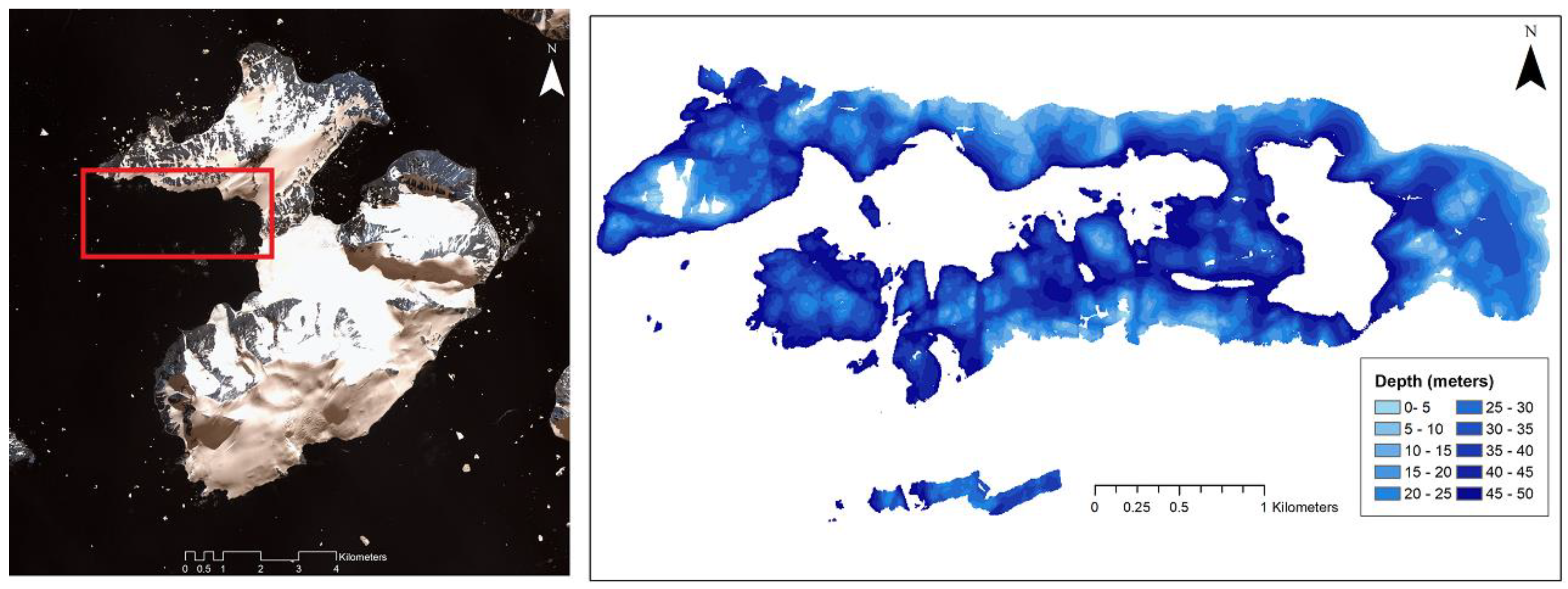
Since the meteorological conditions of Horseshoe Island in Antarctica are quite challenging, the potential to provide data with optical satellites is low. Taking this issue and the year 2019 as a reference, which was the date of the previous Arctic research expedition in which multibeam echosounder (MBE) measurements were performed, an archive search was carried out through the USGS Earth Explorer [43] and Copernicus Open Access Hub [44] portals by defining a time period of 2 years for Landsat 8 and Sentinel 2 satellite images. During the search, cloudiness was not taken into consideration in the first stage, and image selections were made by evaluating the cloudiness rate of the study area based on the results obtained within the scope of the scan results. The initial results of the scan for the period of 2017–2021 provided 5 Landsat 8 and 3 Sentinel 2 cloud-free images (

Table 1. Properties of Landsat 8 and Sentinel 2 images available for the study region.

Scene ID	Platform	Date	Process
LC08_L1GT_219108_20171217_20201016_02_T2	Landsat 8	17.12.2017	L1GT
LC08_L1GT_219108_20180203_20201016_02_T2	Landsat 8	03.02.2018	L1GT
LC08_L1GT_219108_20180219_20201016_02_T2	Landsat 8	19.02.2018	L1GT
LC08_L1GT_219108_20210110_20210307_02_T2	Landsat 8	10.01.2021	L1GT
LC08_L1GT_219108_20210126_20210305_02_T2	Landsat 8	26.01.2021	L1GT
S2A_MSIL1C_20170214T134051_N0204_R038_T19DEE	Sentinel 2	14.02.2018	L1C
S2B_MSIL1C_20190124T131909_N0207_R095_T19DEE	Sentinel 2	24.01.2019	L1C
S2B_MSIL1C_20211129T131909_N0301_R095_T19DEE	Sentinel 2	29.11.2021	L1C

). Among them, Landsat 8 images dated 19 February 2018 and Sentinel 2 images dated 24 January 2019 were used in this study due to their temporal proximity to the in situ MBE data.

Processing levels of the acquired data:

-

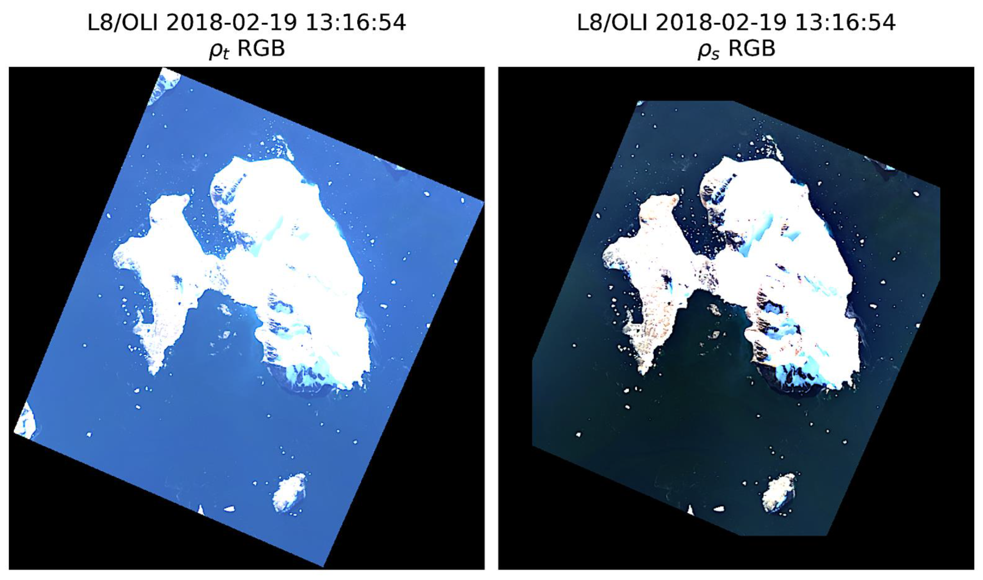
For Landsat 8 data, the L1GT level is radiometrically corrected, geometrically corrected using a limited number of ground points and digital elevation models, and is provided in 16-bit data form. Top of atmosphere (TOA) reflectance values can be obtained from these data by basic coefficient transformations.

-

For Sentinel 2 data, the L1C level is again radiometrically and geometrically corrected, and the TOA reflectance values can be obtained from these data with basic coefficient transformations.

As understood from this information, the images to be used within the scope of the study can only be obtained at basic processing levels, and they need atmospheric correction to reach the surface reflectance values required in satellite-based SDB studies.

The dense MBE data provided as point cloud data with horizontal resolution below 1 m are used as the main training and validation dataset. This dataset was collected with the R2SONIC 2022 instrument during the Turkish Antarctic Expedition (TAE)-III to the region between 29 January–6 March. These data embody a maximum measurement error margin of around 1 m horizontally and 1 cm vertically for 400 m, which is the maximum depth it can measure within its technical capabilities [45]. In this context, a total of 10,000 bathymetric point data, 2500 homogeneously for each 5 m interval for 0–20 m depth, were randomly selected. Of these 10,000 point data, 8000 were used for model training and 2000 were used for validation. During the analysis, 5 m depth intervals were evaluated separately in addition to 0–10 m and 0–20 m intervals for holistic evaluation. The study region and bathymetric model obtained from these data are presented in Figure 1.

Aerosol optical depth (AOD) data that were then measured by ship-borne Microtops II sun photometers through The Maritime Aerosol Network (MAN) component of the Aerosol Robotic Network (AERONET) [46] were obtained from the NASA AERONET website [47] to be used in iCOR and ATCOR atmospheric models.

3. Methodology

This section provides a detailed theoretical background of the processing steps and the algorithms used for the performed SDB mapping. Figure 2 presents the flowchart of the process.

3.1. Atmospheric Correction

Electromagnetic radiation transfer in the atmosphere has significant disturbance effects due to aerosol and gas absorption and Mie and Rayleigh scattering. These effects are particularly important over water areas. Atmospheric path radiance accounts for 85% of electromagnetic energy in the oceans, 94% in darker water bodies, and 60% in waters with high-sediment load [48]. These effects are even more challenging in extreme latitudes and at large solar zenith angles (70°) since the atmospheric path of radiation is longer [49]. In addition, satellites with near nadir viewing angles such as Landsat and Sentinel 2 are affected by sun glint. The adjacency effect is a further issue brought on by atmospheric transmission and radiation scattering. This effect occurs when the scattered radiation from neighboring surfaces is combined with the target radiation and recorded by the sensor, especially when the contrast between the target pixel and its surrounding pixels is highly strong [50]. The adjacency effect is particularly effective at short wavelengths [51]. Horseshoe Island has the characteristics of a region where atmospheric correction is prominent due to its location in the extreme latitude region representing deep and clear ocean water, melting ponds, high contrast by bright ice, and the complex cover type formed by snow surfaces on sea ice and the related neighboring reflection effects.

The atmospheric correction of the satellite images was performed using the ACOLITE, iCOR, and ATCOR algorithms. These algorithms were chosen primarily as they are applicable to both Landsat 8 and Sentinel 2 satellite imagery. The algorithms have also demonstrated a strong linkage with ground-based measurements of water and sea ice in the Arctic, a study area with similarly challenging geographical characteristics that is subject to disturbances [52]. Vanhellemont recommended ACOLITE for marine and ocean surveys based on Landsat and Sentinel 2 due to its correspondence with the AERONET Ocean Color (OC) data [53]. In addition, De Kukelaere et al. reported that the iCOR algorithm provides similar results to ACOLITE [54].

ACOLITE was developed by the Department of Natural Sciences of the Royal Belgian Institute. It consists of processors for atmospheric correction developed especially for applications on water (e.g., handling diffuse sky reflection on the water surface). Information on precipitated water, atmospheric pressure, and ozone concentration used in this algorithm is obtained by connecting to the EARTHDATA platform. Two different atmospheric correction methods are presented within the ACOLITE algorithm. The first is the SWIR-based exponential extrapolation (EXP) method [55], and the second one is the multispectral dark spectrum fitting (DSF) method [56]. The ACOLITE algorithm can also provide continental and maritime aerosol parameterization. Within the scope of the research, it was deemed appropriate to use the DSF method and the Maritime aerosol model by utilizing the findings obtained in Vanhellemont [53]. According to the analysis of AERONET OC data and Landsat and Sentinel 2 images, the DSF model performs better, notably in the blue band. The same study’s results also indicate that the DSF algorithm performs the path reflectance (ρpath) predictions more harmoniously, including clear and turbid coastal waters, inland waters, and terrestrial areas with its tiled working principle. The DSF technique chooses the band with the lowest atmospheric path reflectance automatically, thus minimizing the negative effects of sun glint and adjacency effect. The performance of the DSF algorithm compared with the EXP algorithm is also emphasized by Duan et al. [9].

The iCOR algorithm, previously known as OPERA, can be run by integrating it into the SNAP open-source software provided by ESA. iCOR is an atmospheric correction algorithm for land and sea, and basically consists of 4 work steps [54]: (1) separation of land and water pixels by classification; (2) calculating AOT value for land pixels with the Guanter [57] approach and transferring AOT value to water pixels, assuming a homogeneous atmosphere; (3) neighborhood effect correction with SIMilarity Environment Correction (SIMEC) algorithm; and (4) realization of atmospheric correction on LUT reflectance values obtained using the rural aerosol model and MODTRAN 5 radiative transfer model.

The ATCOR (Atmospheric/Topographic Correction for Satellite Imagery) algorithm uses the MODTRAN 5 radiative transfer model, precomputed LUT tables, and other atmospheric components derived from the image [51,58]. The MODTRAN 5-based LUT tables include four different aerosol models: rural, urban, marine, and desert. In addition, the water vapor (Wv) parameter is parameterized as 6 different values in the range of 0.75–4.11 cm according to season. Ozone concentrations are obtained from a ready-made database. The AOT parameter is determined by the dense dark vegetation algorithm and a user-defined visibility parameter. The aerosol model can be selected by the user, and the Wv parameter is selected by the atmospheric pre-corrected differential absorption algorithm. In the ACTOR algorithm, the adjacency effect is realized by calculating the average reflectance using neighboring pixels.

Within this research, a total of six images were obtained by applying these three atmospheric correction models to Landsat 8 and Sentinel 2 satellite images. The images are produced as surface reflectance (bottom of atmosphere—BoA) information. Figure 3 shows the input ToA image and the BoA view obtained after ACOLITE DSF. Figure 4 demonstrates the difference between the corrected reflectance values obtained with ACOLITE and the pre-correction reflectance values. As seen from these graphs, the differences after correction display a significant difference, especially in the visible region used in the project. The parameter summary of the three algorithms is given in

Table 2. Parameters of the algorithms used in atmospheric correction.

Algorithm	Version	LUT Transfer Model	Aerosol Model	AOT Retrieval	WV Retrieval (cm)	Adjacency Correction	Sun Glint Correction
ACOLITE	20220222	6SV	MARITIME	Dark Spectrum Fitting	User Def: 0.8	acstar3	Fresnel Correction
iCOR	3	MODTRAN 5	RURAL	Image Based (AERO Net)	User Def: 0.8	SIMEC	Fresnel Correction
ATCOR	3	MODTRAN 5	MARITIME	Dense Dark Vegetation	Auto	Average Filter	N/A

.

3.2. Post-Processing

For the purposes of bathymetric analysis, the next step after the atmospheric correction was the sun glint correction. Several studies reported the importance of sun glint removal in SDB mapping [59]. This correction is available inside the ACOLITE and iCOR algorithms; however it is not present in ATCOR. Thus, the method proposed by Hedley et al. [60] was utilized for the ATCOR-corrected images. This method, highly preferred in the literature, is based on the lowest near-infrared reflectance value in the image and performs a regression analysis between itself and the near-infrared reflectance values in all other pixels. As a final step, it reduces the reflectance values of the other bands in the pixels to the water column reflectance value using the calculated regression formula.

The next step of post-processing is to create a land mask and perform land–sea separation. As a result of the profile analysis of the near-infrared band BoA values, the threshold value for the land and sea separation was determined. A mask was created to eliminate terrestrial areas in the near-infrared band, and by applying this mask to the visible bands, images containing only water areas were obtained using the threshold value (Figure 5 left).

In the final step, bottom-feature classification was performed by means of visible band reflectance values. The depth invariant index (DII), introduced by Lyzenga [61] and Green et al. [62], was used for this process. The DII calculation linearizes the logarithmic effect of depth on the reflectance values, and thus makes the reflectance values free from the effect of depth; as such, it allows the identification of similar interactions with bottom topography. The DII transformation is realized by the calculation given in Equation (1).

$$\begin{gathered} DII=ln\left(R_i\right)-\left[\left(k_i/k_j\right)ln\left(R_j\right)\right] \\ \left(k_i/k_j\right)=a+\sqrt{\left(a^2+1\right)} \\ a=\frac{{\sigma }_{ii}-{\sigma }_{jj}}{2{\sigma }_{ij}} \end{gathered}$$

(1)

In this equation, R_i and R_j = the reflectance values of bands i and j, k_i/k_j = ratio attenuation coefficient of bands i and j, σ_ii = variance of band i, σ_jj = variance of band j, and σ_ij = covariance of bands i and j.

This transformation is carried out using the blue and green band reflectance values achieved from the ACOLITE-corrected Landsat 8 OLI image. Following the transformation, the dataset is fed into the elbow method. This method uses a graphic to show the categories that are necessary to successfully describe the entire dataset. It works by calculating the within-cluster sum of square (WCSS), which is the sum of the squared distances between cluster members and the centroid of the cluster. The elbow graph displays WCSS values (on the y-axis) linked with various K values (on the x-axis). The graph’s elbow form indicates the ideal K-value. This area is known as the elbow point. Beyond the elbow point, increasing the value of “K” has no discernible impact on WCSS. In the current study, the elbow is created at K = 4 (Figure 6).

Then, the K-means algorithm was utilized to discriminate the reflective nature of different bottom types, with the predefined optimal number of clusters set at 4. Different classes of bottom types in the region were identified with this process, which is expected to be ground checked with the yet-to-be-analyzed sediment samples that were collected in 2023, (Figure 5 right). Initial analysis identified the loosest sediment cluster in the northwest region (Cluster 1), whereas the stiffest was detected in the upper middle part of the bay (Cluster 4).

3.3. Empirical Models for Bathymetry Estimation

3.3.1. Log Transform (Lyzenga)

The Lyzenga algorithm is based on the correlation relationship between deep water reflectance (R_∞) and total reflectance (R). This method assumes that the ratios of the bottom reflectance values obtained for the two image bands are constant. By deducting the deep-water reflectance value from the derived BoA value, it is projected that the effects of atmospheric scattering and water surface reflectance distortion will be reduced [14,63]. The measured data set also serves as calibration data for the determination of the parameters required during the extraction of bathymetric data from the satellite image as shown in Equation (2):

$$Z={\alpha }_0+\sum _{i=1}^N{\alpha }_{1}ln\left[R\left({\lambda }_i\right)-R_{\infty }\left({\lambda }_i\right)\right]$$

(2)

where “Z” is the satellite-derived depth value, “N” is the number of bands, “α₀” and “α_i” are the coefficients obtained as a result of calibration, “i” is the number of data points (1, 2..., N), “R(λi)” is the perceived reflectance value for the band “i”, and “R_∞” is the deep-water reflectance value for the band “i”. In the literature, green and blue bands are preferred due to their high level of water penetration [64,65].

3.3.2. Log Ratio (Stumpf)

The band ratio method, known as the Stumpf method, basically estimates the depth value by comparing the two bands with the highest penetration values in logarithmic space [15]. Since the "Logarithmic Ratio" assumes that the extinction value increases with increasing depth, it selects the lowest extinction ratio to maintain a constant proportionality with the seafloor radiance. This method, which does not require the removal of the deep-sea column reflection from the system, is reported to have a high performance, especially in operating regions with low reflectivity values as shown in Equation (3):

$$Z=m_1\frac{ln\left(R\left({\lambda }_i\right)\right)}{ln\left(R\left({\lambda }_j\right)\right)}+m_0$$

(3)

where “Z” represents the satellite-derived depth value, “m₁” and “m₀” represent the regression coefficients that give the highest agreement between the depth value and the ratio, and “R(λ_i)” and “R(λ_j)” represent the reflectance values for two different spectral bands. The n component is a constant coefficient and takes the value of 1000 for studies with float reflectance values in the literature. Although the blue-green (BG) band ratio is mostly used for this approach [13,15,30], green-red (GR) and blue-red (BR) combinations were also tested.

3.4. ML-Based Models

3.4.1. Support Vector Machine

Support Vector Machine (SVM), one of the machine learning models used in satellite-based bathymetry applications, is based on the logic of minimizing the prediction reliability within the limits provided by keeping the learning error margin constant based on the data. By mapping the training vectors in a higher dimension, non-linear structures can also be revealed. As seen in analytical models, the relationship between water depth and band ratio in real measurements is far from linearity. In order to model non-linear correspondence, Vojinovic et al. adopted the SVM approach [66]. The SVM method converts the input vector into a multidimensional feature space through nonlinear mapping. Then, it tries to determine the best linear relationship between the multidimensional feature space and water depths as shown in Equation (4):

$$Z=f\left(\frac{ln\left(nR\left({\lambda }_i\right)\right)}{ln\left(nR\left({\lambda }_r\right)\right)}\right)$$

(4)

where Z is the water depth, f is the non-linear function, and the other components are the parameters in the logarithmic ratio method. Although the binary-based SVM algorithm can use different kernels for the transition to multidimensional structure, the radial basis function (RBF), which has been previously accepted for its high generalization capability [66,67], was chosen for this study. These kernel feature vectors, x_i and x_j, are given in Equation (5).

$$k\left(x_i,x_j\right)=e^{-\frac{{‖x_i-x_j‖}^2}{2{\sigma }^2}}$$

(5)

3.4.2. Random Forest

Random Forest (RF) is an ensemble learning technique that creates an extensive number of sub-sample sets at first. To increase the model’s prediction accuracy, it samples the dataset, randomly chooses characteristics in each subset to forecast the decision tree, and then integrates the outcomes of each decision tree’s prediction [9]. This model can be used for classification purposes and regression-based prediction requirements [68]. The RF technique has lately demonstrated greater performance in SDB and effectively represents the non-linear relationship among variables. This method can establish the relationship between directly measured water depths and spectral reflectance values without using any logarithmic transformation [19]. The study was carried out on the Scikit-learn ensemble package in the Python environment with log ratio combinations of red, green, and blue bands as model inputs and the number of random data subsets as 100.

3.4.3. XGBoost

The XGBoost gradient boosting model offers a gradient reduction approach that allows the derivatives of the loss function to be used in optimizing the model prediction values, resulting in a final model that minimizes residual errors. Unlike the RF model, where a large number of decision trees are built in parallel, the primary idea behind this approach is to construct decision trees in a sequential manner. Each model attempts to minimize the errors of the prior one. A new model is constructed based on the errors or residuals of the prior model for this purpose [69]. The XGBoost algorithm differs from general gradient incremental models by its node partitioning, decision tree pruning, and weight adjustment features, and this algorithm mainly improves the loss function via Taylor expansion [70].

3.4.4. Hyperparameter Tuning

The hyperparameters of all three models constructed for bathymetry extraction were optimized using the "Grid Search" approach, and the results are shown in

Table 3. Hyper-parameter set for ML-based models.

SVM	RF	XGBoost
C: 1	bootstrap: True	objective: “reg:squarederror”
gamma: 0.0001	ccp_alpha: 0.0	base_score: 0.5
degree: 3	criterion: squared_error	booster: “gbtree”
cache_size: 200	max_features: 1.0	tree_method: “exact”
coef0: 0.0	min_samples_leaf: 1	colsample_bynode: 1
epsilon: 0.1	min_samples_split: 2	colsample_bytree: 1
kernel: rbf	n_estimators: 100	learning_rate: 0.300000012
max_iter: −1	oob_score: False	n_estimators: 100
shrinking: True	random_state: 45	num_parallel_tree: 1
tol: 0.001	warm_start: False	predictor: “auto”

for each model.

3.5. DL-Based Models

3.5.1. Artificial Neural Networks

Artificial Neural Networks (ANNs) bear non-linear and sample-based structures. Therefore, these assets in the bathymetry extraction process are preferred due to their potential in mapping the non-linear, multi-parameter relationship between the actual depths and corresponding reflectance values from spectral bands. The main contribution of ANNs is that they are immune to optical problems stemming from environmental factors such as turbulence and diversity of bottom topography. The utility of this methodology was first assessed by Ceyhun and Yalcın [16] together with Aster and Quickbird satellite data in Foca/Izmir-Türkiye for depths of up to 45 m and provided fairly accurate bathymetry estimates having a determination coefficient of 0.80. Later in 2016, Patel et al. constructed an ANN-based cascade-forward (CF) back propagation model which was evaluated for single and multi-band applications for turbid waters of Bhopal City Lower Lake [71]. This model delivered bathymetry estimations for depths of up to 12 m with an RMSE of 1.618 m and an R² of 0.9514.

In our study, we utilized a multilayer perceptron (MLP) model for our predictions comprising 3 deep layers having 32, 16, and 8 nodes, respectively; then, we fed the model the log values of blue, green, and red band reflectance values. The "Relu" function was chosen as the activation function for all the layers except for the output layer which was "linear".

3.5.2. Convolutional Neural Networks

Convolutional Neural Networks (CNNs) are renowned for their performance in remotely sensed image classification, such as land use, land cover, and target detection on image scenes such as planes, ships, clouds, etc. Apart from these well-known uses, they pose quite a potential in satellite-derived bathymetry mainly due to their two abilities: (1) the capability of mapping non-linear relations and (2) a local join feature that allows the evaluation of depths of unmeasured points as weighted averages of nearby known depths. In their paper, Lumban-Gaol et al. tested different configurations of CNN architectures to generate SDB models [72]. Based on their analysis, SDB generated from CNN outperforms the linear log transform method, especially when designed with large window sizes. Al Najar et al. demonstrated an initial application of CNN to SDB via measured bathymetric data, wave kinematics, and synthetic replicate images from the Sentinel 2 satellite constellation with an error rate of around 4% [73].

The CNN set-up for our studies had 3 convolution layers with filters 32, 16, and 8 respectively, all of which are subject to a 15% drop-out rate to avoid overfitting. Pooling was utilized with the size of 2. The kernel size was applied as 5 for the 1st 2 convolution layers, whereas the kernel size was 3 for the 3rd layer. The "Relu" function was selected as the activation function for all layers. Finally, the optimizer for the model was set as "Adam" with a learning rate of 0.001.

4. Results

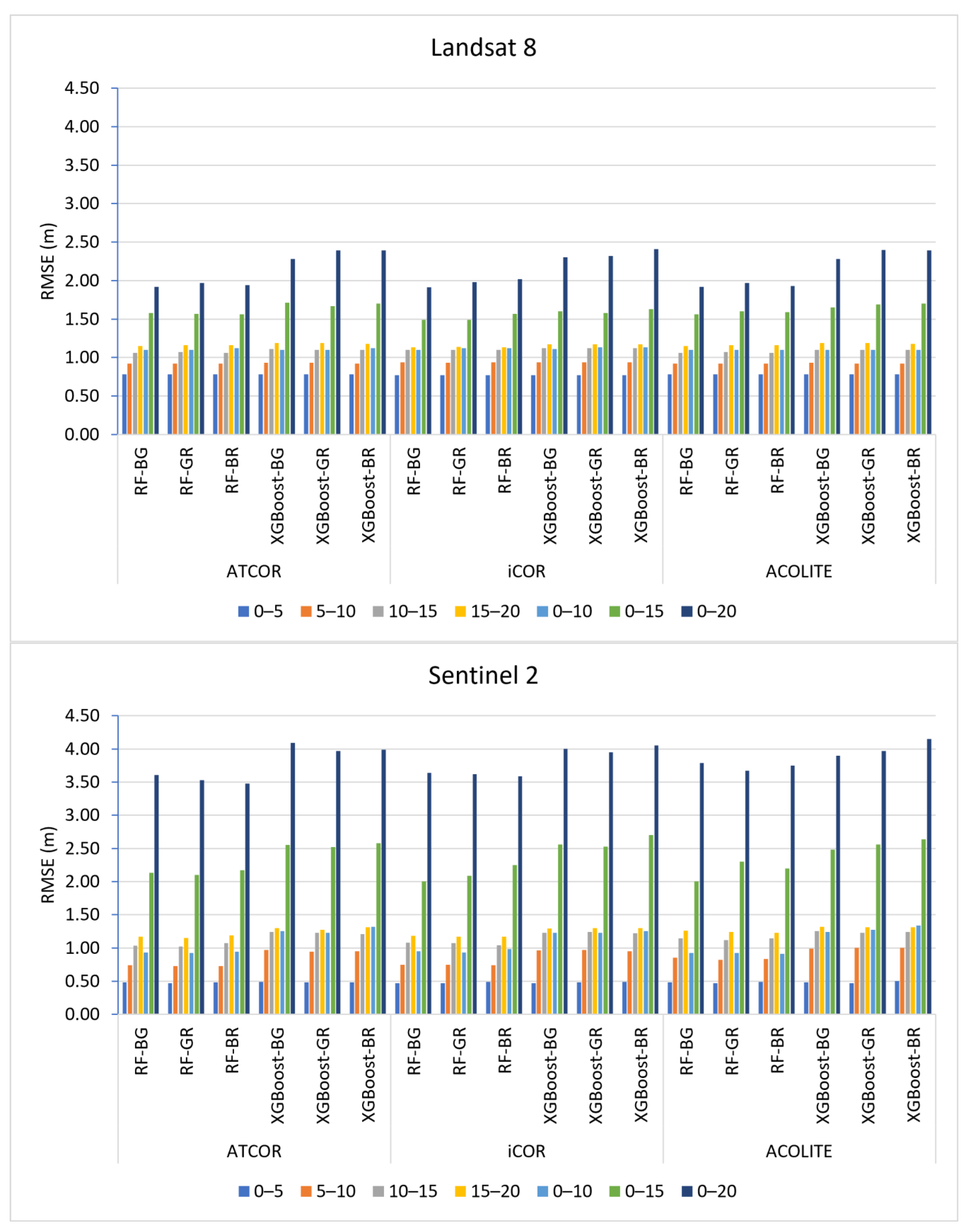
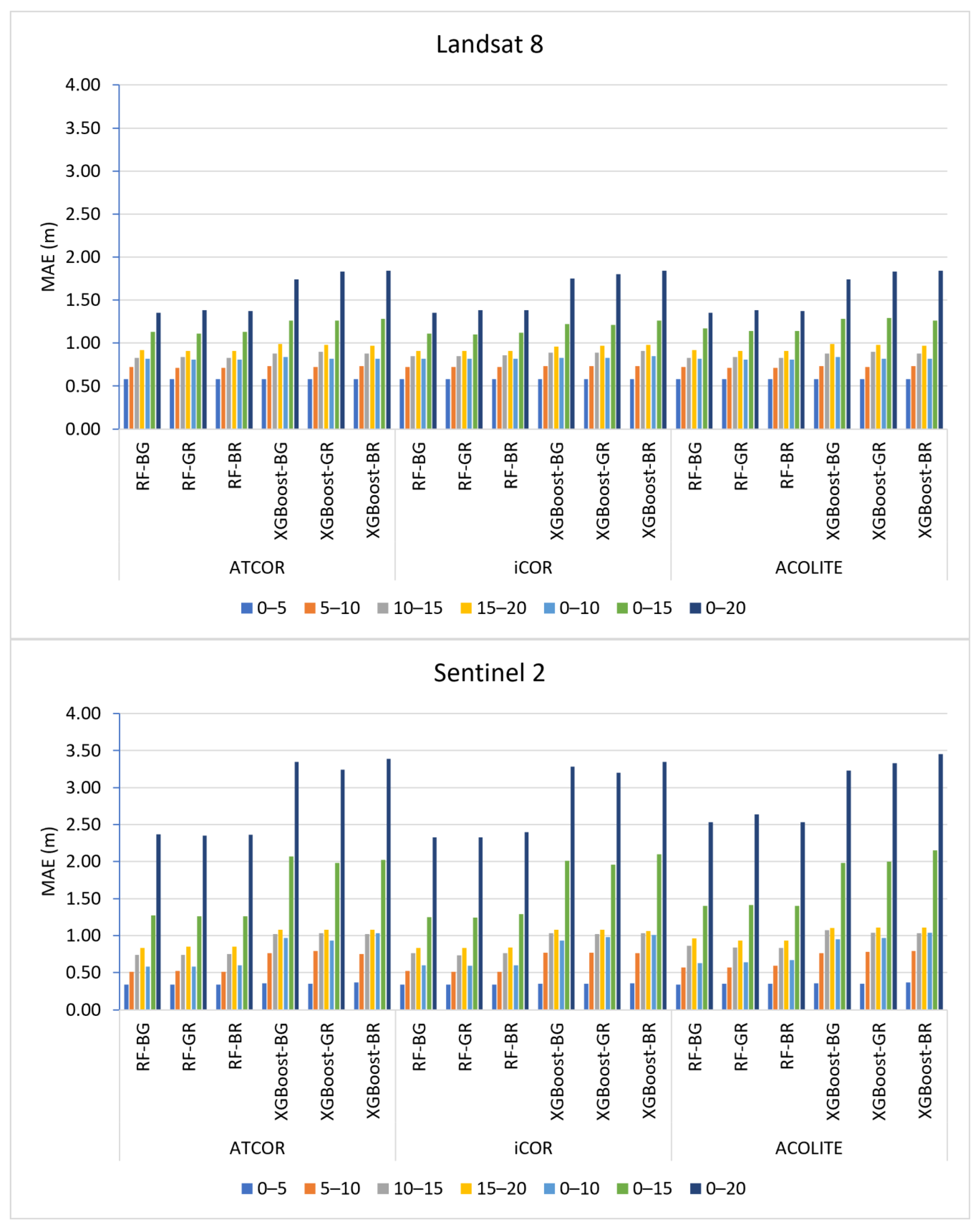
This section presents the analysis results of SDB estimation on the coasts of Horseshoe Island in a comparative structure. The evaluation includes (i) comparing the effects of ACOLITE, ATCOR, and iCOR atmospheric correction algorithms on SDB estimation, (ii) comparing SDB algorithm performances, and (iii) comparing the performances of Landsat 8 and Sentinel 2 visible bands on SBD estimation. The evaluation was carried out for 5 m depth intervals up to 20 m depth. In addition, 0–10 m, 0–15 m, and 0–20 m intervals were examined to check the estimation consistency among increasing depth ranges. Furthermore, all possible visible band pairs were evaluated for Stumpf, SVM, RF, and XGBoost algorithms to investigate the potential effects. ANN- and CNN-based algorithms used RGB images directly in their estimations.

The RMSE- and MAE-based results proved that RF and XGBoost provided the highest performance for the whole sensor, depth, and atmospheric correction configurations. The ANN and CNN algorithms ranked second, and their accuracies were highly close to each other according to the RMSE and MAE values. SVM, Lyzenga, and Stumpf BR algorithms followed the DL-based algorithms again with comparable performances while Stumpf BG and Stumpf GR were ranked last in this comparison (

Table A1. RMSE results for bathymetric models derived from ATCOR-corrected images.

	Landsat 8							Sentinel 2
	0–5	5–10	10–15	15–20	0–10	0–15	0–20	0–5	5–10	10–15	15–20	0–10	0–15	0–20
Stumpf-BG	1.41	1.62	1.51	1.61	3.92	7.00	10.00	1.12	1.37	1.47	1.45	2.70	4.33	5.88
Stumpf-GR	1.18	1.48	1.47	1.53	3.00	5.40	8.00	1.44	1.47	1.60	1.47	3.47	6.00	7.79
Stumpf-BR	1.00	1.34	1.44	1.45	2.26	3.62	4.90	1.00	1.35	1.44	1.45	2.36	3.80	5.24
Lyzenga	1.00	1.33	1.43	1.45	2.17	3.42	4.81	0.96	1.33	1.43	1.45	2.15	3.56	5.00
SVM-BG	1.08	1.35	1.44	1.45	2.52	3.89	5.39	1.08	1.35	1.44	1.45	2.52	3.93	5.39
SVM-GR	1.07	1.35	1.44	1.45	2.52	3.89	5.39	1.08	1.35	1.44	1.45	2.52	3.93	5.39
SVM-BR	1.07	1.35	1.44	1.45	2.50	3.87	5.37	1.08	1.35	1.44	1.45	2.52	3.93	5.39
RF-BG	0.78	0.92	1.06	1.15	1.10	1.58	1.92	0.48	0.74	1.03	1.17	0.93	2.13	3.61
RF-GR	0.78	0.92	1.07	1.16	1.10	1.57	1.97	0.47	0.73	1.02	1.15	0.92	2.10	3.53
RF-BR	0.78	0.92	1.06	1.16	1.12	1.56	1.94	0.48	0.73	1.07	1.19	0.94	2.17	3.48
XGBoost-BG	0.78	0.93	1.11	1.19	1.10	1.71	2.28	0.49	0.97	1.24	1.30	1.25	2.55	4.09
XGBoost-GR	0.78	0.93	1.10	1.19	1.10	1.67	2.39	0.48	0.94	1.23	1.27	1.23	2.52	3.97
XGBoost-BR	0.78	0.92	1.10	1.18	1.12	1.70	2.39	0.48	0.95	1.21	1.31	1.32	2.58	3.99
ANN	0.84	1.30	1.42	1.57	1.69	3.00	4.03	0.89	1.31	1.46	1.44	2.06	3.36	4.74
CNN	0.88	1.29	1.42	1.47	1.87	3.10	4.40	0.90	1.33	1.44	1.44	2.07	3.38	4.76

,

Table A2. RMSE results for bathymetric models derived from iCOR-corrected images.

	Landsat 8							Sentinel 2
	0–5	5–10	10–15	15–20	0–10	0–15	0–20	0–5	5–10	10–15	15–20	0–10	0–15	0–20
Stumpf-BG	1.34	1.56	1.68	1.58	2.70	6.39	10.22	1.06	1.39	1.44	1.45	2.44	3.91	5.61
Stumpf-GR	1.12	1.43	1.53	1.50	2.81	4.80	7.27	1.06	1.36	1.44	1.45	2.41	3.85	5.30
Stumpf-BR	1.02	1.33	1.43	1.45	2.36	3.62	4.91	1.05	1.35	1.44	1.45	2.42	3.90	5.35
Lyzenga	1.02	1.31	1.43	1.45	2.22	3.23	4.58	0.93	1.32	1.43	1.45	2.04	3.29	4.71
SVM-BG	1.08	1.35	1.44	1.45	2.52	3.89	5.38	1.08	1.35	1.44	1.45	2.52	3.91	5.39
SVM-GR	1.07	1.35	1.44	1.45	2.52	3.89	5.39	1.08	1.35	1.44	1.45	2.52	3.90	5.38
SVM-BR	1.06	1.35	1.44	1.45	2.48	3.85	5.38	1.08	1.35	1.44	1.45	2.52	3.91	5.39
RF-BG	0.77	0.94	1.10	1.13	1.10	1.49	1.91	0.47	0.75	1.08	1.18	0.95	2.00	3.64
RF-GR	0.77	0.93	1.10	1.14	1.12	1.49	1.98	0.47	0.75	1.07	1.17	0.93	2.09	3.62
RF-BR	0.77	0.94	1.10	1.13	1.12	1.57	2.02	0.49	0.74	1.04	1.17	0.98	2.25	3.59
XGBoost-BG	0.77	0.94	1.12	1.17	1.11	1.60	2.30	0.47	0.96	1.23	1.29	1.23	2.56	4.00
XGBoost-GR	0.77	0.94	1.12	1.17	1.13	1.58	2.32	0.48	0.97	1.24	1.30	1.23	2.53	3.95
XGBoost-BR	0.77	0.94	1.12	1.17	1.13	1.63	2.41	0.49	0.95	1.22	1.30	1.25	2.70	4.05
ANN	0.81	1.23	1.38	1.45	1.77	2.83	3.97	0.83	1.30	1.43	1.44	2.00	3.40	4.74
CNN	0.86	1.28	1.41	1.47	1.90	2.95	4.03	0.89	1.31	1.44	1.48	2.00	3.41	4.76

,

Table A3. RMSE results for bathymetric models derived from ACOLITE-corrected images.

	Landsat 8							Sentinel 2
	0–5	5–10	10–15	15–20	0–10	0–15	0–20	0–5	5–10	10–15	15–20	0–10	0–15	0–20
Stumpf-BG	1.41	1.62	1.51	1.61	3.92	7.10	10.60	1.06	1.47	1.44	1.45	2.43	3.88	5.38
Stumpf-GR	1.18	1.48	1.47	1.53	3.00	5.47	8.00	1.06	1.37	1.44	1.45	2.43	3.84	5.39
Stumpf-BR	1.00	1.34	1.44	1.45	2.26	3.67	4.90	1.05	1.34	1.44	1.45	2.43	3.86	5.36
Lyzenga	1.01	1.33	1.43	1.45	2.17	3.42	4.81	0.94	1.32	1.43	1.45	2.06	3.31	4.74
SVM-BG	1.08	1.35	1.44	1.45	2.52	3.91	5.39	1.08	1.35	1.44	1.45	2.52	3.86	5.39
SVM-GR	1.08	1.35	1.44	1.45	2.52	3.91	5.39	1.07	1.35	1.44	1.45	2.52	3.86	5.39
SVM-BR	1.07	1.35	1.44	1.45	2.50	3.90	5.37	1.08	1.35	1.44	1.45	2.52	3.86	5.39
RF-BG	0.78	0.92	1.06	1.15	1.10	1.56	1.92	0.48	0.85	1.14	1.26	0.92	2.00	3.79
RF-GR	0.78	0.92	1.07	1.16	1.10	1.60	1.97	0.47	0.82	1.12	1.24	0.92	2.30	3.67
RF-BR	0.78	0.92	1.06	1.16	1.10	1.59	1.93	0.49	0.83	1.14	1.23	0.91	2.20	3.75
XGBoost-BG	0.78	0.93	1.10	1.19	1.10	1.65	2.28	0.48	0.99	1.25	1.32	1.24	2.48	3.90
XGBoost-GR	0.78	0.92	1.10	1.19	1.10	1.69	2.40	0.47	1.00	1.23	1.31	1.27	2.56	3.97
XGBoost-BR	0.78	0.92	1.10	1.18	1.10	1.70	2.39	0.50	1.00	1.24	1.31	1.34	2.64	4.15
ANN	0.82	1.30	1.41	1.44	1.70	2.87	4.02	0.82	1.29	1.44	1.57	2.00	2.12	4.78
CNN	0.81	1.25	1.41	1.44	1.70	3.22	4.16	0.81	1.30	1.43	1.45	2.12	3.45	4.82

,

Table A4. MAE results for bathymetric models derived from ATCOR-corrected images.

	Landsat 8							Sentinel 2
	0–5	5–10	10–15	15–20	0–10	0–15	0–20	0–5	5–10	10–15	15–20	0–10	0–15	0–20
Stumpf-BG	1.38	1.41	1.27	1.29	3.46	6.35	9.37	0.98	1.15	1.31	1.25	2.76	4.64	5.83
Stumpf-GR	1.07	1.29	1.26	1.27	2.49	4.45	6.55	1.27	1.28	1.36	1.26	2.77	4.80	6.25
Stumpf-BR	0.83	1.14	1.25	1.26	2.04	3.19	4.43	0.84	1.15	1.25	1.26	2.07	3.31	4.55
Lyzenga	0.83	1.13	1.25	1.25	1.85	2.89	4.10	0.78	1.13	1.25	1.25	1.81	2.98	4.24
SVM-BG	0.83	1.14	1.25	1.25	2.11	3.37	4.66	0.83	1.14	1.25	1.25	2.11	3.39	4.66
SVM-GR	0.83	1.14	1.25	1.25	2.11	3.37	4.66	0.83	1.14	1.25	1.25	2.11	3.39	4.66
SVM-BR	0.83	1.14	1.25	1.25	2.11	3.37	4.66	0.83	1.14	1.25	1.25	2.11	3.39	4.66
RF-BG	0.58	0.72	0.83	0.92	0.82	1.13	1.35	0.34	0.51	0.74	0.83	0.58	1.27	2.37
RF-GR	0.58	0.71	0.84	0.91	0.81	1.11	1.38	0.34	0.52	0.74	0.85	0.58	1.26	2.35
RF-BR	0.58	0.71	0.83	0.91	0.81	1.13	1.37	0.34	0.51	0.75	0.85	0.60	1.26	2.36
XGBoost-BG	0.58	0.73	0.88	0.99	0.84	1.26	1.74	0.36	0.76	1.02	1.08	0.97	2.07	3.35
XGBoost-GR	0.58	0.72	0.90	0.98	0.82	1.26	1.83	0.35	0.79	1.03	1.08	0.93	1.98	3.24
XGBoost-BR	0.58	0.73	0.88	0.97	0.82	1.28	1.84	0.37	0.75	1.02	1.08	1.03	2.02	3.39
ANN	0.65	1.06	1.22	1.28	1.43	2.30	3.13	0.75	1.12	1.28	1.30	1.58	2.65	3.99
CNN	0.72	1.10	1.32	1.33	1.52	2.62	3.59	0.76	1.15	1.33	1.34	1.64	2.71	3.97

,

Table A5. MAE results for bathymetric models derived from iCOR-corrected images.

	Landsat 8							Sentinel 2
	0–5	5–10	10–15	15–20	0–10	0–15	0–20	0–5	5–10	10–15	15–20	0–10	0–15	0–20
Stumpf-BG	1.34	1.38	1.39	1.28	3.11	5.55	9.31	0.88	1.18	1.26	1.25	2.27	3.80	4.84
Stumpf-GR	0.99	1.25	1.30	1.27	2.25	3.94	5.97	0.86	1.16	1.25	1.25	2.12	3.31	4.61
Stumpf-BR	0.84	1.14	1.25	1.26	2.04	3.21	4.41	0.86	1.15	1.25	1.26	2.13	3.37	4.64
Lyzenga	0.83	1.10	1.24	1.25	1.83	2.75	3.79	0.75	1.11	1.24	1.26	1.69	2.76	3.93
SVM-BG	0.83	1.14	1.25	1.25	2.11	3.38	4.66	0.83	1.14	1.25	1.25	2.11	3.39	4.66
SVM-GR	0.83	1.14	1.25	1.25	2.11	3.38	4.66	0.83	1.14	1.25	1.25	2.11	3.39	4.66
SVM-BR	0.83	1.14	1.25	1.25	2.11	3.38	4.66	0.83	1.14	1.25	1.25	2.11	3.39	4.66
RF-BG	0.58	0.72	0.85	0.91	0.82	1.11	1.35	0.34	0.52	0.76	0.83	0.60	1.25	2.33
RF-GR	0.58	0.72	0.85	0.91	0.82	1.10	1.38	0.34	0.51	0.73	0.83	0.59	1.24	2.33
RF-BR	0.58	0.72	0.86	0.91	0.82	1.12	1.38	0.34	0.51	0.76	0.84	0.60	1.29	2.40
XGBoost-BG	0.58	0.73	0.89	0.96	0.83	1.22	1.75	0.35	0.77	1.03	1.08	0.93	2.01	3.28
XGBoost-GR	0.58	0.73	0.89	0.97	0.83	1.21	1.80	0.35	0.77	1.02	1.08	0.98	1.96	3.20
XGBoost-BR	0.58	0.73	0.91	0.98	0.85	1.26	1.84	0.36	0.76	1.03	1.06	1.01	2.10	3.35
ANN	0.63	0.98	1.20	1.25	1.36	2.15	3.14	0.65	1.06	1.25	1.25	1.68	2.75	4.02
CNN	0.76	1.14	1.32	1.32	1.50	2.39	3.50	0.72	1.11	1.28	1.26	1.75	2.84	4.07

and

Table A6. MAE results for bathymetric models derived from ACOLITE-corrected images.

	Landsat 8							Sentinel 2
	0–5	5–10	10–15	15–20	0–10	0–15	0–20	0–5	5–10	10–15	15–20	0–10	0–15	0–20
Stumpf-BG	1.38	1.41	1.27	1.29	3.46	6.47	9.37	0.84	1.17	1.26	1.25	2.37	4.01	4.97
Stumpf-GR	1.07	1.29	1.26	1.27	2.49	4.50	6.55	0.84	1.16	1.25	1.25	2.12	3.31	4.61
Stumpf-BR	0.83	1.14	1.25	1.26	2.04	3.23	4.43	0.85	1.15	1.25	1.26	2.12	3.33	4.64
Lyzenga	0.83	1.13	1.25	1.25	1.85	2.94	4.10	0.76	1.12	1.24	1.26	1.71	2.74	3.96
SVM-BG	0.83	1.14	1.25	1.25	2.11	3.39	4.66	0.83	1.14	1.25	1.25	2.11	3.35	4.66
SVM-GR	0.83	1.14	1.25	1.25	2.11	3.39	4.66	0.83	1.14	1.25	1.25	2.11	3.35	4.66
SVM-BR	0.83	1.14	1.25	1.25	2.11	3.39	4.66	0.83	1.14	1.25	1.25	2.11	3.35	4.66
RF-BG	0.58	0.72	0.83	0.92	0.82	1.17	1.35	0.34	0.57	0.86	0.96	0.63	1.40	2.53
RF-GR	0.58	0.71	0.84	0.91	0.81	1.14	1.38	0.35	0.57	0.84	0.93	0.64	1.41	2.64
RF-BR	0.58	0.71	0.83	0.91	0.81	1.14	1.37	0.35	0.59	0.83	0.93	0.67	1.40	2.53
XGBoost-BG	0.58	0.73	0.88	0.99	0.84	1.28	1.74	0.36	0.76	1.07	1.10	0.95	1.98	3.23
XGBoost-GR	0.58	0.72	0.90	0.98	0.82	1.29	1.83	0.35	0.78	1.04	1.11	0.97	2.00	3.33
XGBoost-BR	0.58	0.73	0.88	0.97	0.82	1.26	1.84	0.37	0.79	1.03	1.11	1.04	2.15	3.45
ANN	0.65	1.03	1.24	1.25	1.31	2.32	3.13	0.66	1.09	1.24	1.25	1.67	2.72	4.00
CNN	0.77	1.15	1.29	1.30	1.55	2.58	3.56	0.73	1.13	1.32	1.35	1.76	2.75	4.03

). Based on the investigation of the best-performing RF and XGBoost algorithms (Figure 7 and Figure 8), it can be asserted that using different band configurations such as BG, GR, and BR has nearly no impact on the performance of algorithms, except for the Stumpf algorithm where the BR combination provided comparatively stable results. Moreover, notably lower RMSE values were detected in the 0–15 m and 0–20 m intervals than the BG and GR combinations for Landsat 8, while the same situation was not observable for Sentinel 2 (

Table 4. Coefficient of determination (R²) metrics for the RF and XGBoost algorithms across different depth intervals.

	Landsat 8					Sentinel 2
		0–5	0–10	0–15	0–20	0–5	0–10	0–15	0–20
ATCOR	RF-BG	0.46	0.80	0.84	0.87	0.80	0.85	0.71	0.55
	RF-GR	0.46	0.80	0.84	0.86	0.80	0.85	0.72	0.57
	RF-BR	0.46	0.79	0.84	0.87	0.80	0.85	0.70	0.50
	XGBoost-BG	0.46	0.80	0.80	0.80	0.79	0.74	0.58	0.58
	XGBoost-GR	0.46	0.80	0.82	0.79	0.80	0.75	0.57	0.45
	XGBoost-BR	0.46	0.79	0.81	0.80	0.79	0.70	0.57	0.45
iCOR	RF-BG	0.48	0.80	0.85	0.88	0.80	0.83	0.72	0.55
	RF-GR	0.48	0.79	0.86	0.87	0.80	0.86	0.72	0.54
	RF-BR	0.48	0.79	0.84	0.86	0.79	0.84	0.67	0.54
	XGBoost-BG	0.48	0.79	0.83	0.82	0.80	0.75	0.57	0.44
	XGBoost-GR	0.48	0.79	0.84	0.81	0.79	0.74	0.58	0.46
	XGBoost-BR	0.48	0.78	0.82	0.80	0.78	0.72	0.53	0.43
ACOLITE	RF-BG	0.46	0.80	0.84	0.87	0.80	0.80	0.70	0.52
	RF-GR	0.46	0.80	0.84	0.86	0.80	0.80	0.65	0.49
	RF-BR	0.46	0.79	0.84	0.87	0.78	0.80	0.68	0.52
	XGBoost-BG	0.46	0.79	0.83	0.82	0.79	0.74	0.59	0.45
	XGBoost-GR	0.46	0.80	0.82	0.80	0.80	0.73	0.56	0.40
	XGBoost-BR	0.46	0.80	0.82	0.80	0.77	0.70	0.53	0.39

). It is worth mentioning that DL-based models presented the best results in this study. Our experiments demonstrated that changing the loss functions and increasing the model depth (more than three convolutional layers), and feeding the models, either with the log values of RGB bands or a combination of their log ratios, did not provide significant improvements.

The atmospheric correction algorithms had a slight effect on the results, where all sensor and algorithm configurations provided similar performances across different input images resulting from three atmospheric correction algorithms. At this point, it is worth mentioning that, our findings reflect the correlative behavior of surface reflectance values with in situ depths in log space; thus, this finding does not necessarily indicate the similarity of absolute surface reflectance values obtained by these atmospheric correction algorithms. For the ease of application, ACOLITE is more automated and requires no additional input information.

The sensor-based evaluation proved that Sentinel 2 provided higher accuracies in the 0–5 m, 5–10 m, and 0–10 m depth intervals, while the performance of the Landsat 8 was higher for the remaining 5 m intervals and wider depth ranges (0–15 m and 0–20 m). As expected from previous studies, the accuracies reduced with increasing depths; however, ML-based algorithms minimized this increment and provided comparatively consistent mapping performances.

R² is another important indicator that represents the model’s ability to construct the relationship between reflectance and depth. Depth intervals for R² are defined differently than the RMSE, which are 0–5, 0–10, 0–15, and 0–20, to investigate the correlation changes in increasing interval ranges. When the results of correlation analysis were investigated, it was similarly seen that Landsat 8 images provided high and consistent correlation characteristics except for the 0–5 m depth ranges. For Sentinel 2, a decrease in correlation was observable through larger depths such as the 0–15 m and 0–20 m ranges. The SDB algorithms had a small effect, with slightly higher correlations of RF than XGBoost. The results also provided that there is no significant effect of the three atmospheric correction methods on the correlation performance.

The last step of the study was to evaluate the performance in terms of category of zone of confidence (CATZOC) classification. The CATZOC levels are specified in the relevant International Hydrographic Organization (IHO) standard documents [74], which comprise the requisite accuracy in various depth ranges (

Table 5. Accuracy requirements according to IHO CATZOC levels.

CATZOC Level	Depth (m)	Horizontal Accuracy (±m)	Vertical Accuracy (±m)
A1	5	5 + 5% depth	0.55
	10		0.60
	15		0.65
	20		0.70
A2/B	5	20/50	1.10
	10		1.20
	15		1.30
	20		1.40
C	5	500	2.30
	10		2.50
	15		2.80
	20		3.00
D	-	Worse than C	Worse than C

) [27]. SDB results of the study were mainly clustered at Level A2/B and C, while the performance of XGBoost and RF at 0–5 m intervals with Sentinel 2 images satisfied Level A1. Lastly, the performance at 0–20 m, the widest range for all combinations, was evaluated as Level C and Level D (

Table A7. CATZOC classification of bathymetric models derived from ATCOR-corrected images.

	Landsat 8							Sentinel 2
	0–5	5–10	10–15	15–20	0–10	0–15	0–20	0–5	5–10	10–15	15–20	0–10	0–15	0–20
Stumpf-BG	C	C	A2/B	A2/B	D	D	D	A2/B	A2/B	C	A2/B	D	D	D
Stumpf-GR	A2/B	C	A2/B	A2/B	C	D	D	C	C	C	A2/B	D	D	D
Stumpf-BR	A2/B	A2/B	A2/B	A2/B	C	D	D	A2/B	A2/B	A2/B	A2/B	C	D	D
Lyzenga	A2/B	A2/B	A2/B	A2/B	C	D	D	A2/B	A2/B	A2/B	A2/B	C	D	D
SVM-BG	A2/B	A2/B	A2/B	A2/B	C	D	D	A2/B	A2/B	A2/B	A2/B	C	D	D
SVM-GR	A2/B	A2/B	A2/B	A2/B	C	D	D	A2/B	A2/B	A2/B	A2/B	C	D	D
SVM-BR	A2/B	A2/B	A2/B	A2/B	C	D	D	A2/B	A2/B	A2/B	A2/B	C	D	D
RF-BG	A2/B	A2/B	A2/B	A2/B	A2/B	A2/B	A2/B	A1	A1	A2/B	A2/B	A1	A2/B	C
RF-GR	A2/B	A2/B	A2/B	A2/B	A2/B	A2/B	A2/B	A1	A1	A2/B	A2/B	A1	A2/B	C
RF-BR	A2/B	A2/B	A2/B	A2/B	A2/B	A2/B	A2/B	A1	A1	A2/B	A2/B	A2/B	A2/B	C
XGBoost-BG	A2/B	A2/B	A2/B	A2/B	A2/B	A2/B	C	A1	A2/B	A2/B	A2/B	A2/B	C	D
XGBoost-GR	A2/B	A2/B	A2/B	A2/B	A2/B	A2/B	C	A1	A2/B	A2/B	A2/B	A2/B	C	D
XGBoost-BR	A2/B	A2/B	A2/B	A2/B	A2/B	A2/B	C	A1	A2/B	A2/B	A2/B	A2/B	C	D
ANN	A2/B	A2/B	A2/B	A2/B	C	C	D	A2/B	A2/B	A2/B	A2/B	C	C	D
CNN	A2/B	A2/B	C	A2/B	C	C	D	A2/B	A2/B	C	A2/B	C	C	D

,

Table A8. CATZOC classification of bathymetric models derived from iCOR-corrected images.

	Landsat 8							Sentinel 2
	0–5	5–10	10–15	15–20	0–10	0–15	0–20	0–5	5–10	10–15	15–20	0–10	0–15	0–20
Stumpf-BG	C	C	C	A2/B	D	D	D	A2/B	A2/B	A2/B	A2/B	C	D	D
Stumpf-GR	A2/B	C	C	A2/B	C	D	D	A2/B	A2/B	A2/B	A2/B	C	D	D
Stumpf-BR	A2/B	A2/B	A2/B	A2/B	C	D	D	A2/B	A2/B	A2/B	A2/B	C	D	D
Lyzenga	A2/B	A2/B	A2/B	A2/B	C	C	D	A2/B	A2/B	A2/B	A2/B	C	C	D
SVM-BG	A2/B	A2/B	A2/B	A2/B	C	D	D	A2/B	A2/B	A2/B	A2/B	C	D	D
SVM-GR	A2/B	A2/B	A2/B	A2/B	C	D	D	A2/B	A2/B	A2/B	A2/B	C	D	D
SVM-BR	A2/B	A2/B	A2/B	A2/B	C	D	D	A2/B	A2/B	A2/B	A2/B	C	D	D
RF-BG	A2/B	A2/B	A2/B	A2/B	A2/B	A2/B	A2/B	A1	A1	A2/B	A2/B	A2/B	A2/B	C
RF-GR	A2/B	A2/B	A2/B	A2/B	A2/B	A2/B	A2/B	A1	A1	A2/B	A2/B	A1	A2/B	C
RF-BR	A2/B	A2/B	A2/B	A2/B	A2/B	A2/B	A2/B	A1	A1	A2/B	A2/B	A2/B	A2/B	C
XGBoost-BG	A2/B	A2/B	A2/B	A2/B	A2/B	A2/B	C	A1	A2/B	A2/B	A2/B	A2/B	C	D
XGBoost-GR	A2/B	A2/B	A2/B	A2/B	A2/B	A2/B	C	A1	A2/B	A2/B	A2/B	A2/B	C	D
XGBoost-BR	A2/B	A2/B	A2/B	A2/B	A2/B	A2/B	C	A1	A2/B	A2/B	A2/B	A2/B	C	D
ANN	A2/B	A2/B	A2/B	A2/B	C	C	D	A2/B	A2/B	A2/B	A2/B	C	C	D
CNN	A2/B	A2/B	C	A2/B	C	C	D	A2/B	A2/B	A2/B	A2/B	C	D	D

and

Table A9. CATZOC classification of bathymetric models derived from ACOLITE-corrected images.

	Landsat 8							Sentinel 2
	0–5	5–10	10–15	15–20	0–10	0–15	0–20	0–5	5–10	10–15	15–20	0–10	0–15	0–20
Stumpf-BG	C	C	A2/B	A2/B	D	D	D	A2/B	A2/B	A2/B	A2/B	C	D	D
Stumpf-GR	A2/B	C	A2/B	A2/B	C	D	D	A2/B	A2/B	A2/B	A2/B	C	D	D
Stumpf-BR	A2/B	A2/B	A2/B	A2/B	C	D	D	A2/B	A2/B	A2/B	A2/B	C	D	D
Lyzenga	A2/B	A2/B	A2/B	A2/B	C	D	D	A2/B	A2/B	A2/B	A2/B	C	C	D
SVM-BG	A2/B	A2/B	A2/B	A2/B	C	D	D	A2/B	A2/B	A2/B	A2/B	C	D	D
SVM-GR	A2/B	A2/B	A2/B	A2/B	C	D	D	A2/B	A2/B	A2/B	A2/B	C	D	D
SVM-BR	A2/B	A2/B	A2/B	A2/B	C	D	D	A2/B	A2/B	A2/B	A2/B	C	D	D
RF-BG	A2/B	A2/B	A2/B	A2/B	A2/B	A2/B	A2/B	A1	A1	A2/B	A2/B	A2/B	C	C
RF-GR	A2/B	A2/B	A2/B	A2/B	A2/B	A2/B	A2/B	A1	A1	A2/B	A2/B	A2/B	C	C
RF-BR	A2/B	A2/B	A2/B	A2/B	A2/B	A2/B	A2/B	A1	A1	A2/B	A2/B	A2/B	C	C
XGBoost-BG	A2/B	A2/B	A2/B	A2/B	A2/B	A2/B	C	A1	A2/B	A2/B	A2/B	A2/B	C	D
XGBoost-GR	A2/B	A2/B	A2/B	A2/B	A2/B	A2/B	C	A1	A2/B	A2/B	A2/B	A2/B	C	D
XGBoost-BR	A2/B	A2/B	A2/B	A2/B	A2/B	A2/B	C	A1	A2/B	A2/B	A2/B	A2/B	C	D
ANN	A2/B	A2/B	A2/B	A2/B	C	C	D	A2/B	A2/B	A2/B	A2/B	C	C	D
CNN	A2/B	A2/B	A2/B	A2/B	C	C	D	A2/B	A2/B	C	A2/B	C	C	D

).

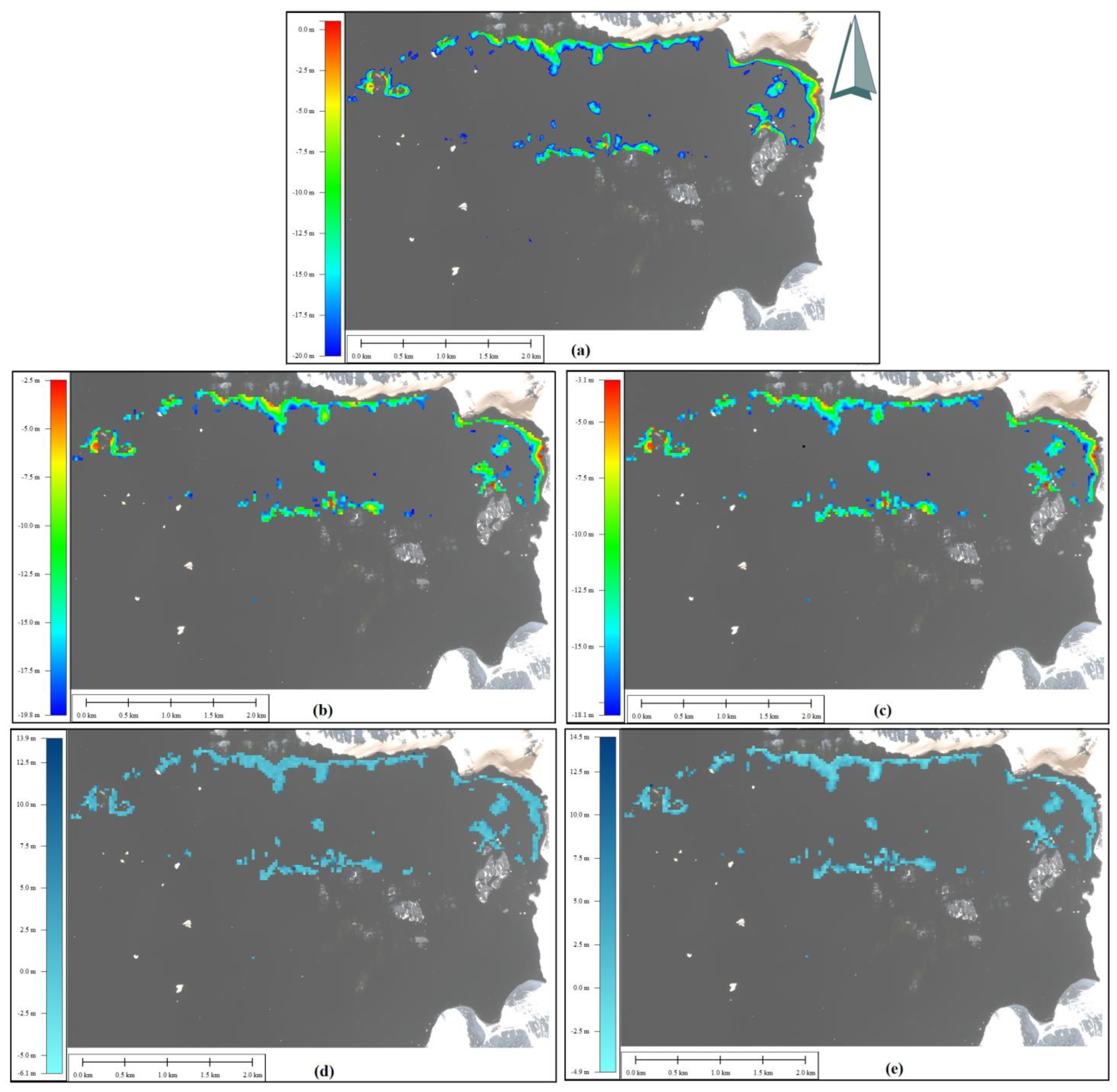
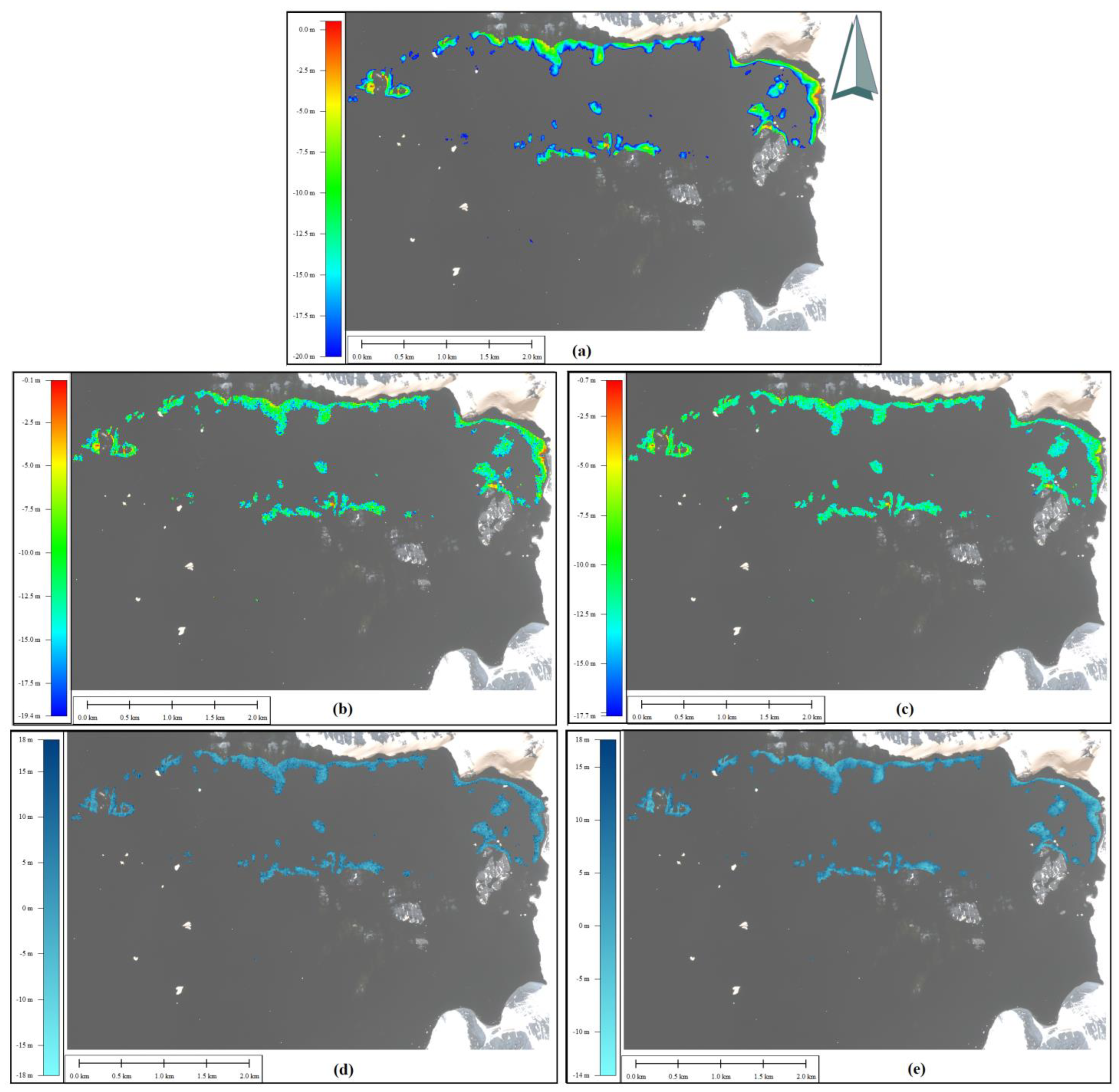
The final products of the 0–20 m range bathymetry inversion were created as raster grid maps for both RF and XGBoost methods, and Landsat 8 and Sentinel 2 images (Figure 9 and Figure 10). In addition, change rasters were also constructed in regard to the grid map of the in situ MBE data for comparison purposes. When these maps are visually investigated, it can be interpreted that both algorithms provide similar results and that they are mostly comparable to the MBE map. The results obtained from Landsat 8 are more in line with MBE in higher depths (Figure 9b,c vs. Figure 10b,c). Additionally, the difference maps from Landsat 8 provided smaller difference ranges (lighter blue) when compared with Sentinel 2 forms (Figure 9d,e vs. Figure 10d,e). Smother boundaries of the Sentinel 2-based maps match well with the MBE data, while the step effect and boundary discontinuities are visible for the Landsat 8-based maps related to higher spatial resolution of the Sentinel 2 images. Lastly, the higher performance of Sentinel 2 in coastal regions (0–5 m depth) is visible on the maps.

5. Discussion

When the results are investigated through the algorithm context, it can clearly be seen that ML- and DL-based algorithms cope well with the non-linear behavior of the reflectance–depth relationship, and provide highly accurate and consistent results for 5 m depth intervals. Although the decrease in accuracy with increasing depth is observable for all methods, this phenomenon is less effective in these models. They also performed well in wider-depth ranges of 0–10 m, 0–15 m, and 0–20 m, indicating their consistent performance. The performance of Lyzenga ranked as the fifth, followed by Stumpf BR and SVM. The worst results were obtained with Stumpf BG and Stumpf GR combinations for Landsat 8, which faced dramatic RMSE and MAE increases in wider depth intervals. While not providing the highest accuracy, SVM was the most consistent method with stable RMSE and MAE values across all atmospheric correction, sensor, and band combinations.

In the sensor context, Landsat 8 provided higher accuracy with lower RMSE and higher R² values in higher depths (greater than 10 m) and wider depth ranges (0–15 and 0–20 m), but faced difficulties in 0–5 m and 0–10 m depth intervals. Sentinel 2 provided better results in 0–5 m, 5–10 m, and 0–10 m intervals; however, its performance dramatically reduced especially in wide depth ranges (higher RMSE, MAE, and lower R²), where it could not build a correlation with in situ MBE data. From these results, it can be commented that Sentinel 2 copes well with depth heterogeneity, which is observable on the shallower parts due to its high spatial resolution, while it exerted a disadvantage in deeper regions where depth became more homogenous. However, higher spatial resolution provides reflectance heterogeneity. This finding points out that, although previous research concluded that higher resolution results in higher accuracy [22,75], the spatial heterogeneity of the depth and conformity of image spatial resolution is another factor to be considered. The findings of Ashphaq et al., 2022, also compared the performance of Landsat 8, Sentinel 2, and ASTER-Terra images in SDB mapping of a turbid coastal water region, and they concluded that they could reach the highest correlation and the lowest accuracy with Landsat 8 images, which supports our findings that spatial resolution is not a direct indicator of higher accuracy [76]. On the other hand, we determined that the advantage of Sentinel 2 is its construction of boundary geometries quite accurately compared with Landsat 8, mainly as a result of its higher spatial resolution.

When the results are analyzed in the context of atmospheric correction, this study’s findings show that, particularly when using ML-based techniques, the effects of the three selected atmospheric correction models on building the relationship between surface reflectance and in situ depth measurements are minimal. This finding conflicts with Duan’s [9] and Abdul Gafoor’s [21] studies, which employed ML-based methods for bathymetric modeling and found noticeable effects of atmospheric correction on modeling, but it is quite consistent with the study conducted by Ceyhun and Yilmaz [16]. It should be highlighted that the proper application of the atmospheric correction to the data is still a factor to be considered. At this point, the ACOLITE model is the most parametrically automated model. In particular, the AOT value calculated by the model agreed with the value (0.030) obtained from the AERONET Microtops Level 2.0 dataset obtained in 2019 in the relevant season. The Wv parameter also agreed with 0.8 cm, which is the average of the summer season between 2019 and 2021. While running the ACOLITE model, the area of interest can be introduced as vector data, and the result data can be obtained only for this area. Although AOT can be calculated as image based for the iCOR model, this approach is primarily based on the calculation of land surfaces; thus, the AOT and Wv values obtained from the AERONET Microtops Level 2.0 dataset were defined manually. The only parameter that can be intervened for ATCOR is Wv, for which 1.0 cm was chosen as the closest value to the Aeronet data. To summarize, iCOR and ATCOR have some limitations related to AOT retrieval and the aerosol model; however, these limitations can be minimized by the use of AERONET OC data.

Although the proposed approaches and the findings of this study point out efficient SDB mapping capabilities in such a region with complex characteristics, it is worth mentioning that SDB is influenced by several factors such as water quality, wave structure, salinity, and illumination conditions related to seasonal differences, which are not directly investigated in this study. Moreover, performance of the recently investigated XGBoost was similar to the RF; however, its advantages on other ML algorithms is mainly observed with high-dimensional datasets [22]. Therefore, its performance should be further checked with a multi-temporal image-based SBD approach. This work used ANN- and CNN-based architectures in SDB mapping, although the performance of recently introduced DL-based architectures remains to be investigated in the future. Lastly, we plan to extend the study to different regions and other sensors for possible performance improvement, and to wider applicability testing of our findings.

6. Conclusions

Several studies have demonstrated the effective use of optical satellite images in satellite-derived bathymetry (SDB) mapping of shallow waters. This study investigated the capability of free-of-charge Landsat 8 and Sentinel 2 satellite images by considering the performances of several SDB algorithms and three atmospheric correction models on SDB mapping in a challenging and complex study region, Horseshoe Island, Antarctic Peninsula, for the first time. The results showed that ML-based RF and XGBoost algorithms are the most effective ones for 5 m depth intervals by providing the highest correlation (R² around 0.80) and lowest RMSE and MAE values. These t2 algorithms also provide reasonable performance in 0–20 m overall depth range, where most of the remaining algorithms failed. When comparing the best-performing RF BG and closest performance ANN for the Landsat 8 image, the MAE reduction was found to be 57% throughout the entire depth range. Thus, these algorithms along with DL-based algorithms can be used for optical SDB studies concerning their large training dataset requirements. CATZOC levels obtained with high-performance models are primarily A2/B and C, which are comparable to previous research employing satellite images with a similar or better spatial resolution. Atmospheric correction algorithms tend to have a limited effect on performance, whereas ACOLITE provided the most automated solution. Landsat 8 provided better results in higher depth intervals such as 10–15 m and 15–20 m and wider depth ranges (0–15 m and 0–20 m), while Sentinel 2 was better in the shallowest areas, where the depth ranges between 0–10 m. The geometry of the boundary lines was represented better with Sentinel 2-based maps by taking advantage of the higher spatial resolution. Further studies are planned to extend this comparison across different regions, to integrate multi-temporal images into methodologies, and to evaluate and integrate much newer DL-based approaches.

References

1. Jawak, S.D.; Luis, A.J. High-resolution multispectral satellite imagery for extracting bathymetric information of Antarctic shallow lakes. In Proceedings of the SPIE 9878, Remote Sensing of the Oceans and Inland Waters: Techniques, Applications, and Challenges, New Delhi, India, 7 May 2016. [Google Scholar]
2. Makowski, C.; Finkl, C.W. Seafloor Mapping along Continental Shelves: Research and Techniques for Visualizing Benthic Environments; Springer: Cham, Switzerland, 2016. [Google Scholar]
3. Robinson, S.A.; Klekociuk, A.R.; King, D.H.; Pizarro Rojas, M.; Zúñiga, G.E.; Bergstrom, D.M. The 2019/2020 summer of Antarctic heatwaves. Glob. Chang. Biol. 2020, 26, 3178–3180. [Google Scholar] [CrossRef] [PubMed]
4. González-Herrero, S.; Barriopedro, D.; Trigo, R.M.; López-Bustins, J.A.; Oliva, M. Climate warming amplified the 2020 record-breaking heatwave in the Antarctic peninsula. Commun. Earth Environ. 2022, 3, 1–9. [Google Scholar] [CrossRef]
5. Turner, J.; Lu, H.; King, J.C.; Carpentier, S.; Lazzara, M.; Phillips, T.; Wille, J. An extreme high temperature event in coastal East Antarctica associated with an atmospheric river and record summer downslope winds. Geophys. Res. Lett. 2022, 49, 1–11. [Google Scholar] [CrossRef]
6. Ashphaq, M.; Srivastava, P.K.; Mitra, D. Review of near-shore satellite derived bathymetry: Classification and account of five decades of coastal bathymetry research. J. Ocean Eng. Sci. 2021, 6, 340–359. [Google Scholar] [CrossRef]
7. Ashphaq, M.; Srivastava, P.K.; Mitra, D. Analysis of univariate linear, robust-linear, and non-linear machine learning algorithms for satellite-derived bathymetry in complex coastal terrain. Reg. Stud. Mar. Sci. 2022, 56, 102678. [Google Scholar] [CrossRef]
8. Vrdoljak, L.; Kilić Pamuković, J. Assessment of Atmospheric Correction Processors and Spectral Bands for Satellite-Derived Bathymetry Using Sentinel-2 Data in the Middle Adriatic. Hydrology 2022, 9, 215. [Google Scholar] [CrossRef]
9. Duan, Z.; Chu, S.; Cheng, L.; Ji, C.; Li, M.; Shen, W. Satellite-derived bathymetry using Landsat-8 and Sentinel-2A images: Assessment of atmospheric correction algorithms and depth derivation models in shallow waters. Opt. Express 2022, 30, 3238–3261. [Google Scholar] [CrossRef]
10. Hodúl, M.; Bird, S.; Knudby, A.; Chénier, R. Satellite derived photogrammetric bathymetry. ISPRS-J. Photogramm. Remote Sens. 2018, 142, 268–277. [Google Scholar] [CrossRef]
11. Yunus, A.P.; Dou, J.; Song, X.; Avtar, R. Improved bathymetric mapping of coastal and lake environments using Sentinel-2 and Landsat-8 images. Sensors 2019, 19, 2788. [Google Scholar] [CrossRef]
12. Casal, G.; Monteys, X.; Hedley, J.; Harris, P.; Cahalane, C.; McCarthy, T. Assessment of empirical algorithms for bathymetry extraction using Sentinel-2 data. Int. J. Remote Sens. 2019, 40, 2855–2879. [Google Scholar] [CrossRef]
13. Chu, S.; Cheng, L.; Ruan, X.; Zhuang, Q.; Zhou, X.; Li, M.; Shi, Y. Technical Framework for Shallow-Water Bathymetry with High Reliability and No Missing Data Based on Time-Series Sentinel-2 Images. IEEE Trans. Geosci. Remote Sens. 2019, 57, 8745–8763. [Google Scholar] [CrossRef]
14. Lyzenga, D.R. Shallow-water bathymetry using combined lidar and passive multispectral scanner data. Int. J. Remote Sens. 1985, 6, 115–125. [Google Scholar] [CrossRef]
15. Stumpf, R.P.; Holderied, K.; Sinclair, M. Determination of water depth with high-resolution satellite imagery over variable bottom types. Limnol. Oceanogr. 2003, 48 Pt 2, 547–556. [Google Scholar] [CrossRef]
16. Ceyhun, Ö.; Yalçın, A. Remote sensing of water depths in shallow waters via artificial neural networks. Estuar. Coast. Shelf Sci. 2010, 89, 89–96. [Google Scholar] [CrossRef]
17. Misra, A.; Vojinovic, Z.; Ramakrishnan, B.; Luijendijk, A.; Ranasinghe, R. Shallow Water Bathymetry Mapping Using Support Vector Machine (SVM) Technique and Multispectral Imagery. Int. J. Remote Sens. 2018, 39, 4431–4450. [Google Scholar] [CrossRef]
18. Manessa, M.D.M.; Kanno, A.; Sekine, M.; Haidar, M.; Yamamoto, K.; Imai, T.; Higuchi, T. Satellite-Derived Bathymetry Using Random Forest Algorithm and Worldview-2 Imagery. Geoplanning 2016, 3, 117. [Google Scholar] [CrossRef]
19. Sagawa, T.; Yamashita, Y.; Okumura, T.; Yamanokuchi, T. Satellite derived bathymetry using machine learning and multi-temporal satellite images. Remote Sens. 2019, 11, 1155. [Google Scholar] [CrossRef]
20. Mudiyanselage, S.S.J.D.; Abd-Elrahman, A.; Wilkinson, B.; Lecours, V. Satellite-derived bathymetry using machine learning and optimal Sentinel-2 imagery in South-West Florida coastal waters. GIScience Remote Sens. 2022, 59, 1143–1158. [Google Scholar] [CrossRef]
21. Gafoor, F.A.; Al-Shehhi, M.R.; Cho, C.-S.; Ghedira, H. Gradient Boosting and Linear Regression for Estimating Coastal Bathymetry Based on Sentinel-2 Images. Remote Sens. 2022, 14, 5037. [Google Scholar] [CrossRef]
22. Susa, T. Satellite Derived Bathymetry with Sentinel-2 Imagery: Comparing Traditional Techniques with Advanced Methods and Machine Learning Ensemble Models. Mar. Geod. 2022, 45, 435–461. [Google Scholar] [CrossRef]
23. Nagamani, P.V.; Chauhan, P.; Sanwlani, N.; Ali, M.M. Artificial neural network (ann) based inversion of benthic substrate bottom type and bathymetry in optically shallow waters—Initial model results. J. Indian Soc. Remote Sens. 2012, 40, 137–143. [Google Scholar] [CrossRef]
24. Liu, S.; Wang, L.; Liu, H.; Su, H.; Li, X.; Zheng, W. Deriving bathymetry from optical images with a localized neural network algorithm. IEEE Trans. Geosci. Remote 2018, 56, 5334–5342. [Google Scholar] [CrossRef]
25. Dickens, K.; Armstrong, A. Machine Learning of Derived Bathymetry and Coastline Detection. SMU Data Sci. Rev. 2019, 2, 4. [Google Scholar]
26. Ai, B.; Wen, Z.; Wang, Z.; Wang, R.; Su, D.; Li, C.; Yang, F. Convolutional Neural Network to Retrieve Water Depth in Marine Shallow Water Area from Remote Sensing Images. IEEE J. Sel. Top. Appl. Earth Obs. Remote Sens. 2020, 13, 2888–2898. [Google Scholar] [CrossRef]
27. Wan, J.; Ma, Y. Shallow Water Bathymetry Mapping of Xinji Island Based on Multispectral Satellite Image using Deep Learning. J. Indian Soc. Remote Sens. 2021, 49, 2019–2032. [Google Scholar] [CrossRef]
28. Zhou, W.; Tang, Y.; Jing, W.; Li, Y.; Yang, J.; Deng, Y.; Zhang, Y. A Comparison of Machine Learning and Empirical Approaches for Deriving Bathymetry from Multispectral Imagery. Remote Sens. 2023, 15, 393. [Google Scholar] [CrossRef]
29. Hernandez, W.J.; Armstrong, R.A. Deriving bathymetry from multispectral remote sensing data. J. Mar. Sci. Eng. 2016, 4, 8. [Google Scholar] [CrossRef]
30. Caballero, I.; Stumpf, R.P. Atmospheric correction for satellite-derived bathymetry in the Caribbean waters: From a single image to multi-temporal approaches using Sentinel-2A/B. Opt. Express 2020, 28, 11742–11766. [Google Scholar] [CrossRef]
31. Basith, A.; Prastyani, R. Evaluating ACOMP, FLAASH and QUAC on Worldview-3 for satellite derived bathymetry (SDB) in shallow water. Geod. Cartogr. 2020, 46, 151–158. [Google Scholar] [CrossRef]
32. Antarctic Wheather. Available online: https://www.antarctica.gov.au/about-antarctica/weather-and-climate/weather/ (accessed on 5 January 2023).
33. Pan, X.L.; Li, B.F.; Watanabe, Y.W. Intense Ocean freshening from melting glacier around the Antarctica during early twenty-first century. Sci. Rep. 2022, 12, 383. [Google Scholar] [CrossRef]
34. Adusumilli, S.; Fricker, H.A.; Medley, B.; Padman, L.; Siegfried, M.R. Interannual variations in meltwater input to the Southern Ocean from Antarctic ice shelves. Nat. Geosci. 2020, 13, 616–620. [Google Scholar] [CrossRef] [PubMed]
35. Nitsche, F.; Jacobs, S.; Larter, R.; Gohl, K. Bathymetry of the Amundsen Sea continental shelf: Implications for geology, oceanography, and glaciology. Geochem. Geophys. Geosyst. 2007, 8, Q10009. [Google Scholar] [CrossRef]
36. Graham, A.G.; Nitsche, F.; Larter, R.D. An improved bathymetry compilation for the Bellingshausen Sea, Antarctica, to inform ice-sheet and ocean models. Cryosphere 2011, 5, 95–106. [Google Scholar] [CrossRef]
37. Smith, J.; Nogi, Y.; Spinoccia, M.; Dorschel, B.; Leventer, A. A bathymetric compilation of the cape Darnley region, East Antarctica. Antarctic Sci. 2021, 33, 548–559. [Google Scholar] [CrossRef]
38. Yang, J.; Guo, J.; Greenbaum, J.S.; Cui, X.; Tu, L.; Li, L.; Jong, L.M.; Tang, X.; Li, B.; Blankenship, D.D.; et al. Bathymetry beneath the amery ice shelf, East Antarctica, revealed by airborne gravity. Geophys. Res. Lett. 2021, 48, e2021GL096215. [Google Scholar] [CrossRef]
39. Dorschel, B.; Hehemann, L.; Viquerat, S.; Warnke, F.; Dreutter, S.; Tenberge, Y.S.; Accettella, D.; An, L.; Barrios, F.; Bazhenova, E.; et al. The International Bathymetric Chart of the Southern Ocean Version 2. Sci. Data 2022, 9, 275. [Google Scholar] [CrossRef] [PubMed]
40. Roy, D.P.; Wulder, M.A.; Loveland, T.R.; Woodcock, C.E.; Allen, R.G.; Anderson, M.C.; Helder, D.; Irons, J.R.; Johnson, D.M.; Kennedy, R. Landsat-8: Science and product vision for terrestrial global change research. Remote Sens. Environ. 2014, 145, 154–172. [Google Scholar] [CrossRef]
41. Alganci, U. Dynamic Land Cover Mapping of Urbanized Cities with Landsat 8 Multi-temporal Images: Comparative Evaluation of Classification Algorithms and Dimension Reduction Methods. ISPRS Int. J. Geo-Inf. 2019, 8, 139. [Google Scholar] [CrossRef]
42. Pacheco, A.; Horta, J.; Loureiro, C.; Ferreira, Ó. Retrieval of nearshore bathymetry from Landsat 8 images: A tool for coastal monitoring in shallow waters. Remote Sens. Environ. 2015, 159, 102–116. [Google Scholar] [CrossRef]
43. Earth Explorer; 2000; FS; 083-00; Geological Survey (U.S.). Available online: https://earthexplorer.usgs.gov/ (accessed on 1 January 2022).
44. Copernicus Open Access Hub. Copernicus, ESA. 2019. Available online: https://scihub.copernicus.eu/dhus (accessed on 1 January 2022).
45. Tükenmez, E.; Gülher, E.; Kaya, Ö.; Polat, H.F. Bathymetric analysis of Lystad Bay, Horseshoe Island by Using High Resolution Multibeam Echosounder Data. J. Nav. Sci. Eng. 2022, 18, 281–303. [Google Scholar]
46. Smirnov, A.B.N.; Holben, I.; Slutsker, D.M.; Giles, C.R.; McClain, T.F.; Eck, S.M.; Sakerin, A.; Macke, P.; Croot, G.; Zibordi, P.K.; et al. Jourdin Maritime Aerosol Network as a component of Aerosol Robotic Network. J. Geophys. Res. 2009, 114, D06204. [Google Scholar] [CrossRef]
47. Nasa Aeronet Maritime Aerosol Network (MAN)—Version 2. Available online: https://aeronet.gsfc.nasa.gov/new_web/maritime_aerosol_network.html (accessed on 16 January 2022).
48. IOCCG. Atmospheric Correction for Remotely-Sensed Ocean-Colour Products. 2010. Available online: http://www.ioccg.org/reports/report10.pdf (accessed on 1 January 2022).
49. IOCCG. Ocean Colour Remote Sensing in Polar Seas. In Reports of the International Ocean-Colour Coordinating Group, No. 16; Babin, M., Arrigo, K., Bélanger, S., Forget, M.-H., Eds.; International Ocean-Colour Coordinating Group: Dartmouth, NS, Canada, 2015; p. 130. [Google Scholar]
50. Sterckx, S.; Knaeps, S.; Kratzer, S.; Ruddick, K. SIMilarity Environment Correction (SIMEC) applied to MERIS data over inland and coastal waters. Remote Sens. Environ. 2015, 157, 96–110. [Google Scholar] [CrossRef]
51. Richter, R.; Schläpfer, D. Atmospheric/Topographic Correction for Satellite Imagery: ATCOR-2/3 User Guide; DLR IB 565-01/17; ResearchGate: Wessling, Germany, 2017. [Google Scholar]
52. König, M.; Hieronymi, M.; Oppelt, N. Application of Sentinel-2 MSI in Arctic Research: Evaluating the Performance of Atmospheric Correction Approaches Over Arctic Sea Ice. Front. Earth Sci. 2019, 7, 22. [Google Scholar] [CrossRef]
53. Vanhellemont, Q. Adaptation of the dark spectrum fitting atmospheric correction for aquatic applications of the Landsat and Sentinel-2 archives. Remote Sens. Environ. 2019, 225, 175–192. [Google Scholar] [CrossRef]
54. De Keukelaere, L.; Sterckx, S.; Adriaensen, S.; Knaeps, E.; Reusen, I.; Giardino, C.; Bresciani, M.; Hunter, P.; Neil, C.; Van der Zande, D.; et al. Atmospheric correction of landsat-8/OLI and sentinel-2/MSI data using iCOR algorithm: Validation for coastal and inland waters. Eur. J. Remote Sens. 2018, 51, 525–542. [Google Scholar] [CrossRef]
55. Vanhellemont, Q.; Ruddick, K. Turbid wakes associated with offshore wind turbines observed with Landsat 8. Remote Sens. Environ. 2014, 145, 105–115. [Google Scholar] [CrossRef]
56. Vanhellemont, Q.; Ruddick, K. Atmospheric correction of meter-scale optical satellite data for inland and coastal water applications. Remote Sens. Environ. 2018, 216, 586–597. [Google Scholar] [CrossRef]
57. Guanter, L. New Algorithms for Atmospheric Correction and Retrieval of Biophysical Parameters in Earth Observation. Application to ENVISAT/MERIS Data. Ph.D. Thesis, Universitat de Valéncia, Departament de Física de la Terra i Termodinàmica, Valencia, Spain, 2006. [Google Scholar]
58. Berk, A.; Anderson, G.; Acharya, P.; Bernstein, L.; Muratov, L.; Lee, J.; Fox, M.; Adler-Golden, S.; Chetwynd, J.; Hoke, M. MODTRANTM5: 2006 update. In Proceedings of the SPIE 6233, Algorithms and Technologies for Multispectral, Hyperspectral, and Ultraspectral Imagery XII, Orlando, FL, USA, 17 April 2006. [Google Scholar]
59. Goodman, J.A.; Lee, Z.; Ustin, S. Influence of atmospheric and sea-surface corrections on retrieval of bottom depth and reflectance using a semi-analytical model: A case study in Kaneohe Bay, Hawaii. Appl. Opt. 2008, 47, F1–F11. [Google Scholar] [CrossRef]
60. Hedley, J.D.; Harborne, A.R.; Mumby, P.J. Technical note: Simple and robust removal of sun glint for mapping shallow-water benthos. Int. J. Remote Sens. 2005, 26, 2107–2112. [Google Scholar] [CrossRef]
61. Lyzenga, D.R. Passive remote sensing techniques for mapping water depth and bottom features. Appl. Opt. 1978, 17, 379–383. [Google Scholar] [CrossRef]
62. Green, E.; Mumby, P.; Edwards, A.; Clark, C. Remote Sensing: Handbook for Tropical Coastal Management; United Nations Educational Scientific and Cultural Organization (UNESCO): Paris, France, 2000. [Google Scholar]
63. Lyzenga, D.R.; Malinas, N.P.; Tanis, F.J. Multispectral bathymetry using a simple physically based algorithm. IEEE Trans. Geosci. Remote Sens. 2006, 44, 2251–2259. [Google Scholar] [CrossRef]
64. Kibele, J.; Shears, N.T. Nonparametric empirical depth regression for bathymetric mapping in coastal waters. IEEE J. Sel. Top. Appl. Earth Observ. Remote Sens. 2016, 9, 5130–5138. [Google Scholar] [CrossRef]
65. Shen, X.; Jiang, L.; Li, Q. Retrieval of Near-Shore Bathymetry from Multispectral Satellite Images Using Generalized Additive Models. IEEE Geosci. Remote Sens. Lett. 2019, 16, 922–926. [Google Scholar] [CrossRef]
66. Vojinovic, Z.; Abebe, Y.; Ranasinghe, R.; Vacher, A.; Martens, P.; Mandl, D.; Frye, S.; Van Ettinger, E.; De Zeeuw, R. A machine learning approach for estimation of shallow water depths from optical satellite images and sonar measurements. J. Hydroinform. 2013, 15, 1408–1424. [Google Scholar] [CrossRef]
67. Girosi, F.; Poggio, T. Networks and the best approximation property. Biol. Cybern. 1990, 63, 169–176. [Google Scholar] [CrossRef]
68. Breiman, L. Random forests. Mach. Learn. 2001, 45, 5–32. [Google Scholar] [CrossRef]
69. Friedman, J. Greedy function approximation: A gradient boosting machine. Ann. Stat. 2001, 29, 1189–1232. [Google Scholar] [CrossRef]
70. Chen, T.; Guestrin, C. XGBoost: A Scalable Tree Boosting System. In Proceedings of the 22nd ACM SIGKDD International Conference on Knowledge Discovery and Data Mining, San Francisco, CA, USA, 13–17 August 2016; pp. 785–794. [Google Scholar]
71. Patel, A.; Katiyar, S.K.; Prasad, V. Bathymetric mapping of Bhopal City Lower Kake using IRS-P6: LISS-4 imagery and artificial neural network technique. J. Indian Soc. Remote Sens. 2016, 44, 605–616. [Google Scholar] [CrossRef]
72. Lumban-Gaol, Y.A.; Ohori, K.A.; Peters, R.Y. Satellite-derived bathymetry using convolutional neural networks and multispectral sentinel-2 images. The International Archives of the Photogrammetry, Remote Sensing and Spatial Information Sciences. In Proceedings of the XXIV ISPRS Congress, Nice, France, 5–9 July 2021; Volume XLIII-B3-2021. [Google Scholar]
73. Al-Najar, M.; Thoumyre, G.; Bergsma, E.W.J.; Almar, R.; Benshila, R.; Wilson, D.G. Satellite derived bathymetry using deep learning. Mach. Learn. 2021, 112, 1107–1130. [Google Scholar] [CrossRef]
74. International Hydrographic Organization (IHO). S-67 Mariners’ Guide to Accuracy of Depth Information in Electronic Navigational Charts (ENC) (Edition 1.0.0, September 2020). Available online: https://iho.int/en/standards-and-specifications (accessed on 1 December 2022).
75. Ahola, R.R.; Chenier, M.S.; Horner, B. The impact of sensors for satellite derived bathymetry within the Canadian arctic. Geomatica 2020, 74, 46–64. [Google Scholar] [CrossRef]
76. Ashphaq, M.; Srivastava, P.K.; Mitra, D. Evaluation and performance of satellite-derived bathymetry algorithms in turbid coastal water: A case study of Vengurla rocks. Indian J. Mar. Sci. 2022, 51, 310–321. [Google Scholar] [CrossRef]
Figure 1. The coverage area of the bathymetric data obtained by the MBE (left) and 5 m grid resolution bathymetry model produced from these data (right).
Remotesensing 15 02568 g001
Figure 2. Flowchart of bathymetric model extraction from an optical satellite image.
Remotesensing 15 02568 g002
Figure 3. RGB presentation of the pre-correction ToA (left) and post-ACOLITE correction BoA (right) images for Landsat 8 satellite imagery from 2018.
Remotesensing 15 02568 g003
Figure 4. Reflectance curve plots (left) and difference plots (right) before and after ACOLITE correction.
Remotesensing 15 02568 g004
Figure 5. Shallow-water mask (left) and bottom feature classification map (right) of the study region.
Remotesensing 15 02568 g005
Figure 6. Result of the elbow method indicating the optimal number of clusters as 4.
Remotesensing 15 02568 g006
Figure 7. RMSE distribution of RF and XGBoost models for whole sensor, atmospheric correction, and depth configurations.
Remotesensing 15 02568 g007
Figure 8. MAE distribution of RF and XGBoost models for whole sensor, atmospheric correction, and depth configurations.
Remotesensing 15 02568 g008
Figure 9. (a) Bathymetric data up to 20 m collected by MBE; (b) L8-based random forest bathymetry extraction; (c) L8-based XGBoost bathymetry extraction; (d) surface difference of RF-based and MBE-based bathymetric data; and (e) surface difference of XGBoost-based and MBE-based bathymetric data.
Remotesensing 15 02568 g009
Figure 10. (a) Bathymetric data up to 20 m collected by MBE; (b) S2-based random forest bathymetry extraction; (c) S2-based XGBoost bathymetry extraction; (d) surface difference of RF-based and MBE-based bathymetric data; and (e) surface difference of XGBoost-based and MBE-based bathymetric data.
Remotesensing 15 02568 g010