Article

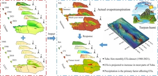
Estimation and Spatiotemporal Evolution Analysis of Actual Evapotranspiration in Turpan and Hami Cities Based on Multi-Source Data

1
College of Geographical and Remote Science, Xinjiang University, Urumqi 830017, China
2
Xinjiang Key Laboratory of Oasis Ecology, Xinjiang University, Urumqi 830017, China
3
Key Laboratory of Smart City and Environment Modelling of Higher Education Institute, Urumqi 830017, China
*
Author to whom correspondence should be addressed.
These authors contributed equally to this work.
Remote Sens. 2023, 15(10), 2565; https://doi.org/10.3390/rs15102565
Submission received: 4 April 2023 / Revised: 8 May 2023 / Accepted: 11 May 2023 / Published: 14 May 2023

Abstract

:
The accurate inversion of actual evapotranspiration (ETa) at a regional scale is crucial for understanding water circulation, climate change, and drought monitoring. In this study, we produced a 1 km monthly ETa dataset for Turpan and Hami, two typical arid cities in northwest China, using multi-source remote sensing data, reanalysis information, and the ETMonitor model from 1980 to 2021. We analyzed the spatiotemporal variation of ETa using various statistical approaches and discussed the impact of climate and land use and cover changes (LUCC) on ETa. The results show the following: (1) the estimation results correlate well with ETa products on monthly scales (coefficient of determination (R2) > 0.85, root mean square error (RMSE) < 15 mm/month) with high reliability. (2) The ETa values were spatially distributed similarly to precipitation and LUCC, with the multi-year (1980–2021) average of 66.31 mm and a slightly fluctuating downward trend (−0.19 mm/a). (3) During the 42-year period, 63.16% of the study area exhibited an insignificant decrease in ETa, while 86.85% experienced pronounced fluctuations (coefficient of variation (CV) > 0.20), and 78.83% will show an upward trend in the future. (4) ETa was significantly positively correlated with precipitation (94.17%) and insignificantly positively correlated with temperature (55.81%). The impact of human activities showed an insignificant decreasing trend (85.41%). Additionally, the intensity of ETa varied considerably among land types, with the largest for cropland (424.12 mm/a). The results of the study have implications for promoting the rational allocation of regional water resources and improving water use efficiency in arid zones.

Graphical Abstract

1. Introduction

Evapotranspiration (ET) is a crucial component of the global energy exchange through the water cycle and the carbon cycle [1]. In arid regions, it can release over 80% of water to the atmosphere. According to the Sixth Assessment Report (AR6) of the Intergovernmental Panel on Climate Change, the global surface temperature (TEM) reached its highest level in 125,000 years between 2011 and 2020, and the water cycle rate rose dramatically, leading to significant and complex changes in ET. Furthermore, according to the report of the 20th National Congress of the Communist Party of China, we should “advance green development and harmonious coexistence between humans and nature”, and the human–water relationship is an important manifestation of the human–nature relationship [2]. Therefore, the accurate estimation and monitoring of ET in arid areas are of great significance for assessing the supply–demand balance of water resources, guiding agricultural irrigation, and preventing desertification [3]. However, accurate ET information or datasets with continuous coverage and medium-high resolution in space (i.e., 1 km) and time are still lacking in the Turpan-Hami region.
Traditional ET estimations are based on point-scale observations made using instruments such as evaporation pans, lysimeters, and flux towers to derive ET from the underlying surface of Earth. However, these data cannot effectively reflect surface ET at regional scales and cannot meet the needs of planning for the rational development and utilization of regional water resources [4]. Remote sensing (RS) technology provides a new way to obtain ET data [5], and it has spawned a variety of ET estimation models [6,7,8], including SEBAL [9], TSEB [10], HSEB [11], and EEOET [12]. RS data can provide surface parameters such as temperature, net radiation, and vegetation index with a high spatiotemporal resolution, and models can then be used to describe the physical relationships between ET and these parameters. By combining RS data and models, regional-scale ET can be estimated more effectively, and factors such as different land-cover types, seasonal changes, and climatic conditions can be considered.
However, these models also have their own defects and uncertainties, such as ignoring the physiological processes of vegetation, soil moisture stress, and cloud effects. For this reason, Hu and Jia developed the ETMonitor model, which comprehensively considers energy balance, water balance, and the physiological processes of vegetation [13,14]. The ETMonitor model uses multi-source satellite observations and introduces variables such as the soil moisture (SM) index, vegetation temperature index, and cloud cover index in parameterizing the soil–atmosphere energy and water exchange [15]. This model can effectively invert daily ETa and its components at a 1 km global scale, and it has been validated against the results of other models.
The development of RS cloud-computing platforms [16,17] has prompted the creation of RS evapotranspiration products such as MOD16A2, GLASS, GLEAM, and PML–V2. These products have their own benefits and drawbacks: data such as GLEAM and GLDAS have long coverage times and wide applicability but low spatial resolution; MOD16A2 has a higher spatiotemporal resolution (500 m/8-day) and is widely used [18], but it is value-free in areas without vegetation cover; PML-V2 is a relatively new ETa data product (2000.02–2020.12) that is more applicable in arid zones [19].
In recent decades, the northwestern arid area of China has been affected by global climate change, especially the increase in temperature [20]. The cities of Turpan and Hami are ecologically fragile and sensitive to climate change, and warming, retreating glaciers, melting permafrost, the increased water cycle, and significant changes in ET in the region have significant impacts on regional socioeconomic development and the protection of the ecological environment. Warming leads to an increase in potential evapotranspiration (ETp), but ETa depends on water availability [21]. Moreover, since the implementation of reforestation in 2000, the local forestry and fruit industries have grown, and a protective forest system—mainly for wind and sand control—has been built. However, vegetation restoration may lead to increased water loss through transpiration, and the spatiotemporal dynamics and attribution of ETa in Tuha are still unclear.
In light of the above, in this work, using multi-source RS and reanalysis data, the ETMonitor model [13] was applied to produce a monthly ETa dataset for Tuha from 1980 to 2021, and the characteristic patterns of spatiotemporal changes in ETa at the raster scale of Tuha were analyzed by combining Sen’s slope estimator, the Mann–Kendall (MK) trend test, the coefficient of variation (CV), and the Hurst index. The effects of climate factors and land use on ETa are discussed in this paper with a view to providing a reference for ETa estimation, sustainable water resource utilization, and the protection of the ecological environmental in Tuha and other similar subsurface areas.

2. Materials and Methods
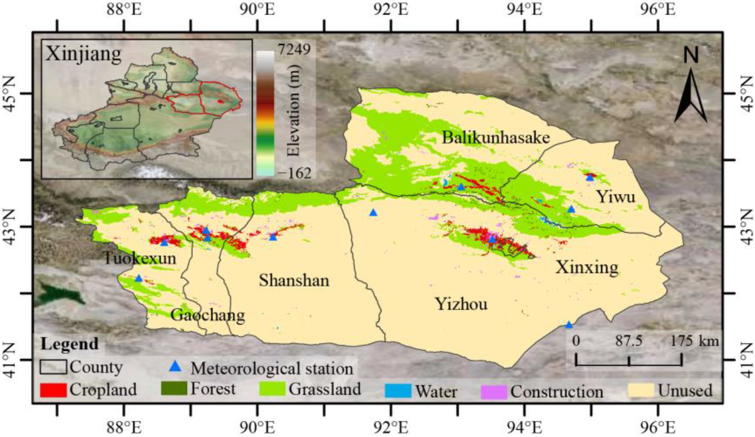
2.1. Study Area

The Turpan-Hami region (Tuha, 41°18′–43°43′N, 86°40′–96°04′E) is located in the east-central part of Xinjiang, China (Figure 1), and comprises the cities of Turpan, Xinxing, and Hami. Tuha belongs to a region with a typical arid continental climate and a distinct and fragile mountain-oasis-desert ecosystem.
Tuha is located in the hinterland of Eurasia with seasonal differences in precipitation (PRCP, 16–35 mm/a) and evaporation (2314 mm/a). Additionally, the region’s long sunshine hours (3360.3 h) [22], high effective cumulative temperature (>5300 °C), low relative humidity, strong wind force, and other characteristics aggravate the occurrence and impact of natural catastrophes such as sandstorm, drought, salinization, etc. Small rivers, springs, and canals are important water sources in this area due to the uneven distribution of water resources in space and time [23]. However, Tuha also faces multiple water shortages caused by resource and engineering factors.
Tuha is one of the key areas of the Third Xinjiang Scientific Examination and the key construction area of the “Three Bases and One Passage” in Xinjiang. The region is abundant in coal, oil, and gas resources [24], but its topography is undulating and meteorological stations are sparse, which makes the estimation of water cycle elements challenging. Therefore, in such an intricate and sensitive ecosystem, the analysis of surface energy balance and water cycle processes is of great practical importance for understanding and predicting climate change in the region and its impact on water resources and the ecological environment.

2.2. Data

2.2.1. Satellite Data

To quantitatively estimate the ETa of Tuha at a 1 km scale, we used the ETMonitor model with multi-source RS and reanalysis data (Table 1) as input parameters. Since Moderate Resolution Imaging Spectroradiometer (MODIS) products are more influenced by clouds and spatiotemporal discontinuities [13], we adopted Global Land Surface Satellite (GLASS) products as the main data source and used Python, the Internet Download Manager (IDM), and the MODIS Reprojection Tool (MRT) to batch download GLASS data with the stitching row numbers h24v04 and h25v04, and brought them into the model to estimate ETa. Among these, because of the lack of data for recent years from GLASS products, the data from MODIS products were used instead.
To ensure the validity of ETa estimation in Tuha, an accuracy evaluation is necessary. However, due to the paucity of actual measurements of ETa data in Tuha, we mainly evaluated the accuracy by comparing the results with existing ETa products. Although a variety of global-scale ETa products have been released, such as MOD16A2, GLEAM, and SSEBop (Simplified Surface Energy Balance operational), these products either have low spatial resolution or have large regions of missing values in the desert or Gobi areas of Tuha. In view of this, based on the worldwide development frontiers of ETa simulation research, four sets of relatively new ETa products were selected as references (Table 1). Because these products have differing spatial resolutions, to ensure the accuracy of regional-scale evaluation, they needed to be resampled to 1 km using bilinear interpolation and translated into unified units of mm/month.

2.2.2. Meteorological and LUCC Data
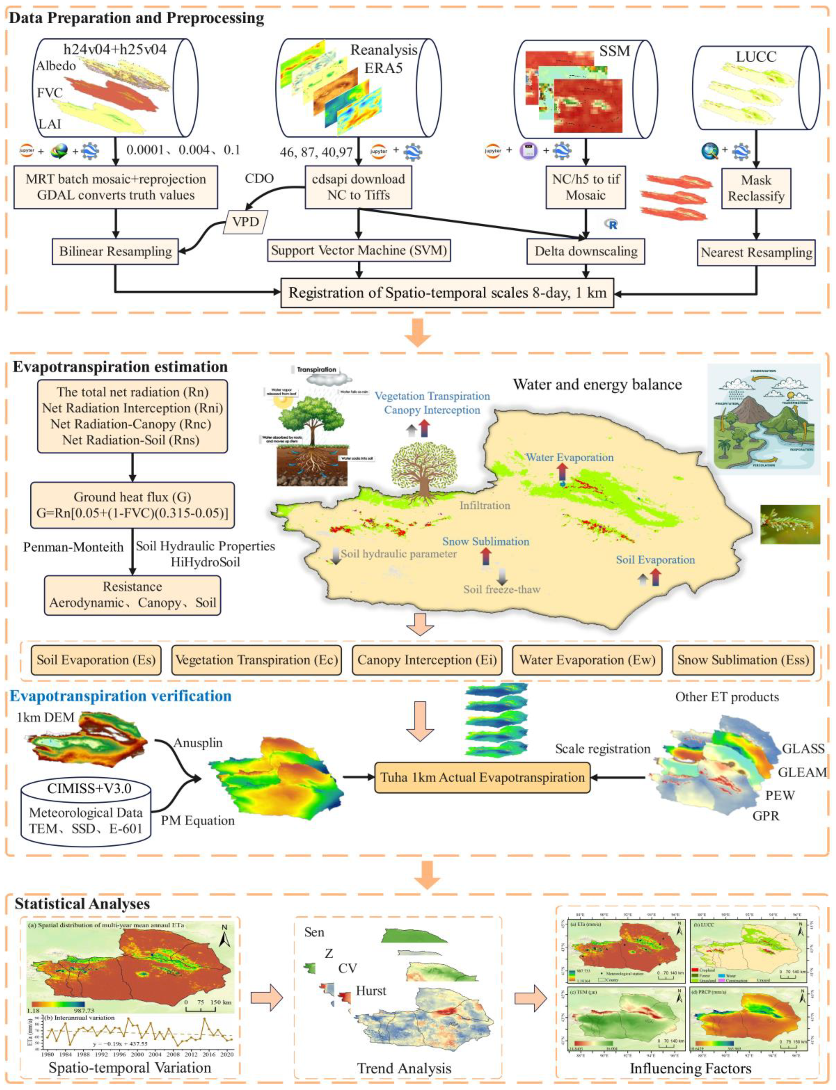
To ensure the integrity of the meteorological data time series and the uniformity of the distribution of meteorological stations, we obtained the TEM, WIN, sunshine duration (SSD), relative humidity (RHU), and evaporation (EVP) for 11 stations in Tuha from 1980 to 2020 from the China Meteorological Data Network and Xinjiang Provincial Meteorological Bureau (Table 2). Linear interpolation was used for missing values, and the EVP Ice Age conversion factor was 0.55 [38]. Then, reference crop evapotranspiration (ET0) data were calculated for each site using the Penman–Monteith (PM) formula [39]. Finally, ANUSPLIN 4.37 [40] combined with digital elevation model (DEM) interpolation was used to generate the Tuha 1 km monthly ET0-PM data, which were used to aid in verifying the estimated ETa.
LUCC is a crucial element of global climate change research as it significantly impacts changes in ETa. The CNLUCC [31] is a remote sensing monitoring product that provides comprehensive data on the current status of land use in China from 1980 to 2020, issued by the Chinese Academy of Sciences. It is considered to be one of the most authoritative, complete, and precise datasets relating to the current status of LUCC in China [44]. Wuhan University has collected the CLCD, which is the most detailed and complete dataset in China for the 30 m resolution of land use and land cover change from 1985 to 2021 [30]. These two datasets are characterized by a higher resolution, more accurate categorization systems, and richer information on changes than other sources. To reduce uncertainty in the ETa analysis arising from using multiple data sources, we have chosen these two datasets to examine the differences in ETa for different land classes in Tuha. To maintain data integrity and consistency with the CNLUCC, we converted the CLCD from the 30 m to 1 km resolution using nearest-neighbor resampling.

2.3. Methods

2.3.1. Algorithm of ET

The ETMonitor model is an ETa model, capable of simulating processes such as snow sublimation, that has been validated and applied in different climatic regions and land surface types, so this paper ran the model with reference to the calculation method (Table 3) and parameter values [45,46,47,48,49,50] proposed by Zheng et al. However, the random forest (RF) in the article could not be implemented due to the lack of real soil measurement data in Tuha, so this paper used Delta for downscaling based on the gap-free SSM data after ERA5 filled the ESA CCI, combined with the 1 km daily SM datasets [51] in China published by Song et al. and then estimated resistance (Figure 2). This approach provides an idea and method for estimating ETa in arid areas where there is a scarcity of measured data, and it can be used as a reference for other similar studies.

2.3.2. Precision Evaluation

In order to accurately evaluate the efficacy of the ETa estimation method in Tuha, it is essential to use appropriate parameters as measures. As such, a set of parameters (Table 4) including the correlation coefficient (R), coefficient of determination (R2), root mean square error (RMSE), bias, and Kling-Gupta efficiency (KGE) [53] were identified as suitable measures for assessing the accuracy of the ETa estimation method.

2.3.3. Statistical Analysis

Using methods (Table 5) such as Sen, MK, CV, Hurst, and a partial correlation analysis based on MATLAB R2022a, a comprehensive and in-depth analysis was conducted in Tuha’s ETa from 1980 to 2021. This revealed the spatiotemporal variation characteristics, fluctuations, future trends, and attributions with a view to providing a reference for understanding water resource changes in Tuha.

3. Results

3.1. Accuracy Evaluation

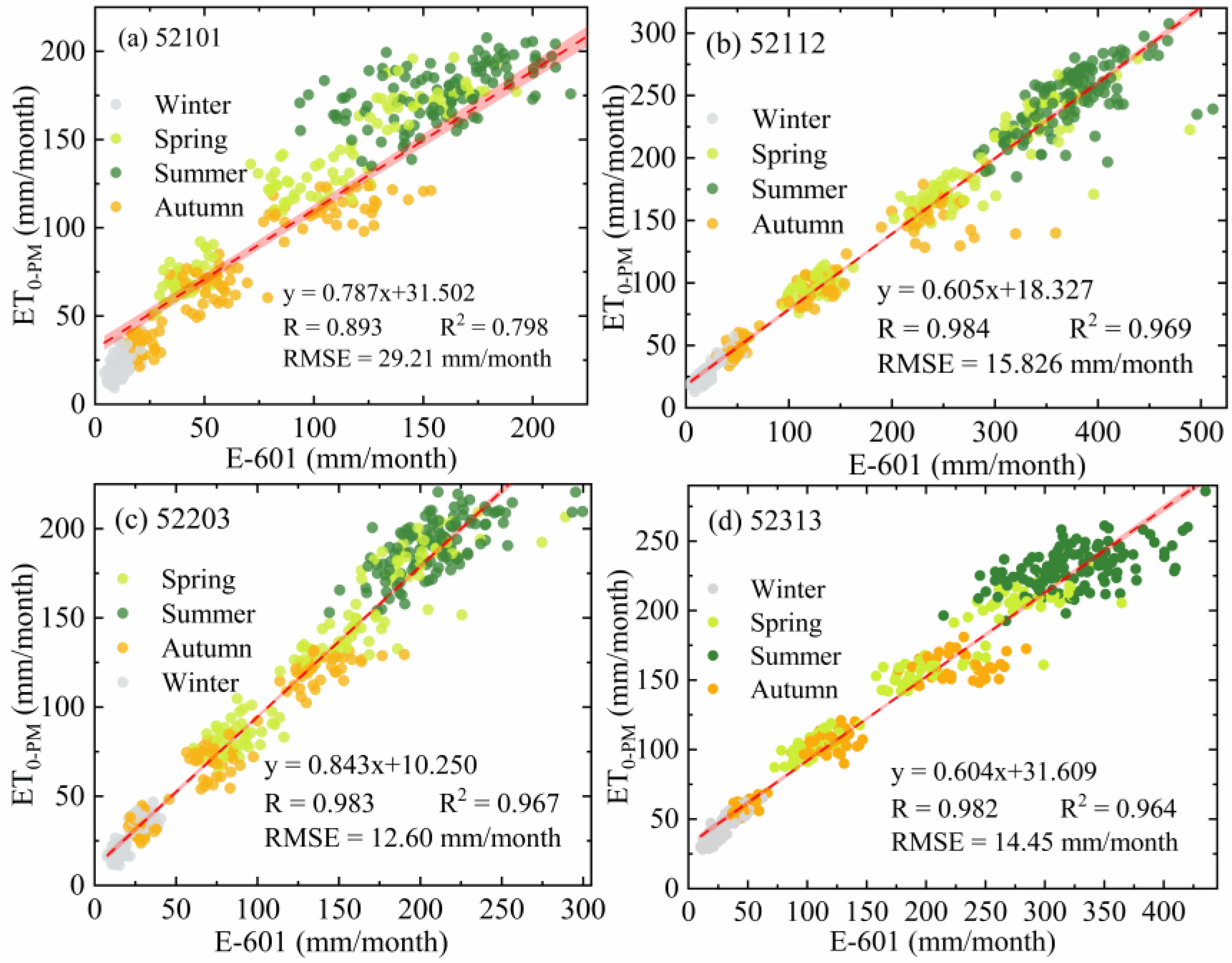
3.1.1. Comparison with ET0-PM

Because of the dearth of measured ETa data in Tuha, to validate the estimated ETa, we first used data from E-601 evaporators (measuring water surface evaporation) and ET0-PM to assist with the validation. Although their values are much higher than ETa in arid areas such as Tuha, a comparison between them has a certain degree of validity under the conditions of a scarcity of measured data [54].
To ensure the accuracy of ET0-PM, we selected four meteorological stations with complete and typical time-series data from 1980 to 2018 for Tuha distributed across distinct land-use types (grassland, construction, and unused land). We compared ET0-PM with E-601 data from these stations on a monthly scale for the analysis (Figure 3). The results showed that the correlation between ET0-PM and E-601 was high, with the R values all greater than 0.85 and R2 values ranging from 0.79 to 0.97. The spatiotemporal trends showed that ET0-PM was higher than E-601 in areas with more vegetation, such as grasslands and croplands, and this might be related to the effects of plant transpiration. In general, the ET0-PM values coincided relatively well with the E-601 data, with RMSE ranging from 12.6 to 29.21 mm/month.
The actual crop evapotranspiration (ETc) was calculated by multiplying the reference crop evapotranspiration (ET0) by the crop coefficient (KC). The KC is a dimensionless attenuation coefficient that takes into account the effects of growth status, environmental differences, and other factors on ETc. According to the main vegetation types and their characteristics within the Turpan-Hami region, and referring to the KC table recommended by FAO, combined with the relevant research on oasis in arid zones [55], the value of KC at Balikun station was determined to be 0.38 in this article comprehensively.
Then, we compared the calculated ETa values with the actual evapotranspiration of crops. Figure 4a describes the relationship between ETc and the estimation results in Balikun station, with ETc on the horizontal axis and ETa on the vertical axis. The fitted line demonstrates a certain degree of correlation between the two, with good statistical parameters. A strong correlation was indicated by R = 0.84, whereas ETa could explain 71.20% of the deviation in ETc as demonstrated by R2 = 0.71. Prediction errors with a small RMSE of 14.15 mm/month and relatively good prediction results with KGE = 0.58 were observed. As shown in Figure 4b, the lower edge and median of ETc were higher than ETa, indicating that ETc was more robust than ETa. This may be due to the fact that the crop releases a large amount of water vapor through the stomata and leaf surfaces, which increases the ambient humidity and thus promotes ET. Meanwhile, the upper edge of ETc was lower than Eta. This may be due to the hot and humid climate in the summer, when the crop is stimulated by light and heat to release more water, leading to an increase in ETc and a corresponding increase in ETa. Conversely, in the winter, when temperatures are low and humidity is low, ET is minimal. The graph also shows that ET varied with the seasons: it was highest in the summer, lowest in the winter, and in between in the spring and autumn.
The overall trend of ETc and ETa at Balikun station from 1980 to 2020 was increasing, and the former was higher than the latter (Figure 4c). This difference may be caused by various factors, such as interannual climate change, the crop cultivation area, and the crop species. For example, a dry climate can lead to a decrease in ET for all plants, while an increase in the acreage of a crop can affect ETc more significantly. The trends in ETa and ETc were the same in some years and different in others, and this may be influenced by a variety of factors such as climate, acreage, and variety. For example, the temperature and rainfall in some years will have similar effects on the amount of ET for all plants, making the trends of ETa and ETc the same, while in other years they will be different because the changes in different crop varieties and planting areas lead to different trends. From Figure 4d, it can be seen that the difference between ETa and ETc shows a decreasing trend from south to north. In the local enlargement near Balikun station, the higher ETa was accompanied by a slightly higher ETc. In summary, ETa in the Turpan-Hami region is generally stable, with higher values in the Balikun station area, while the difference between ETc and ETa is small.

3.1.2. Comparisons with Other ETa Datasets

A correlation analysis between the estimated ETa for Tuha and the existing ET products (GLEAM, PEW, GPR, and GLASS) on a monthly scale is shown in Figure 5. The results show that the estimated ETa had a high positive correlation with the existing ETa products, with the highest correlations with GPR and PEW, reaching 0.95 and 0.92, respectively. In terms of bias and KGE, the estimated ETa values were closer to GLEAM (−8.26 and 0.85 mm/month), while they were closer to PEW in terms of RMSE. There are large differences in comparison to the GLASS v4.0 data, which may be due to the errors caused by summing up 8-day composites into months. These comparative analyses indicate that although there were some discrepancies between the estimated ETa and previous research results due to the different data sources, lengths of time series, and other factors, they showed good correlation on a monthly scale and the annual fluctuations between them. Therefore, the estimated ETa values satisfied the requirements of the existing ET products [56] and can be used to explore the spatiotemporal variation characteristics of ETa in Tuha.
Our estimated results exhibit spatial distribution patterns comparable to those of the other four ETa products, as shown in Figure 6. In the Turpan-Hami region, the average ETa from 2000–2018 obtained from our study was 64.33 mm/a, somewhat less than that of GLEAM v3.6a (77.05 mm/a), GPR (102.63 mm/a), and PEW (92.12 mm/a), yet higher than the mean of GLASS v4.0 (51.38 mm/a). The estimated results show lower ETa values in most barren compared to ETa products such as GLEAM, GLASS, and PEW. Considerable variabilities were found in the spatial distribution of ETa within the Turpan city center and Hami northwestern regions, which could be attributed to differences in model structures and input data quality.
The ETMonitor model considers soil-surface evaporation, canopy-interception water evaporation, and plant transpiration to better reflect the non-uniformity of desert and oasis substrates [13]. Although the simulated values obtained from this model are generally low when compared to ET0-PM and other existing ET products, their accuracy is sufficient for regional-scale studies. Therefore, the estimated ETa can be used to reveal the spatial and temporal dynamic characteristics of regional ET, especially in Tuha, where observation sites are sparse.

3.2. Spatiotemporal Variations of ETa

3.2.1. Annual Scale

Elucidating the spatial and temporal variation patterns of ET in arid regions provides a crucial guideline for studying regional hydrology, agricultural water demand, irrigation planning, and water resource management. Consequently, in this work, a typical representative of the arid zone in northwest China, namely Tuha, was selected as the research object, and the ETa of Tuha from 1980 to 2021 was quantified and analyzed using the ETMonitor model.
The results indicate that there are significant spatial variations in Tuha’s annual ETa (Figure 7a), and these are intimately connected to PRCP and LUCC. For the past 42 years, the low ETa zone in the Turpan-Hami region has been widely distributed. The spatial pattern exhibits a gradual decrease from the mountainous areas towards the surrounding plains. This is partly because ETa in arid areas is principally driven by moisture status, which directly affects the water content of surface soil and increases the magnitude of ETa [57]. The western mountainous areas of Tuha have abundant PRCP due to the influence of the westerly circulation bringing moist flow from the Atlantic Ocean to the windward slopes (Figure 7c); in contrast, the plains have comparatively low PRCP. Although Tuha has a high altitude, strong solar radiation, and sufficient energy for ET, its inland location, sparse PRCP, and low soil moisture result in a huge proportion of Tuha having low ETa values.
LUCC also impacts the spatial pattern of ETa in Tuha (Figure 1). ETa was found to be higher in woodlands and grasslands in mountainous areas such as the Tianshan and Bogda mountains, while it was lower in sparsely vegetated areas and unutilized land in the Igo and Tuha basins. The vegetation cover and soil moisture of agricultural land in oasis areas are higher than those in the sparsely vegetated areas at the edges of oases due to artificial cultivation and irrigation, causing significant spatial heterogeneity in ETa. In contrast, ETa values are lower than 200 mm in high mountainous areas such as the Altai mountains; this can be explained by the greater ability of these ice-covered mountains to reflect short-wavelength radiation, meaning there is less energy available for evaporation. This distribution is opposite to that of the distinct altitudes of Tuha because of disparities in the dynamical and thermal properties of the different land coverings, leading to a redistribution of energy in ground–air interactions.
To illustrate the characteristics of changes in ETa, TEM, and PRCP in Tuha from 1980 to 2021, a one-dimensional linear regression analysis of their regional means was conducted. Figure 8a displays the annual dynamics in the spatial barycenter of ETa in the Turpan-Hami area, which indirectly indicated variations in water resource distribution in the region. The latitude and longitude of the ETa center of gravity showed an insignificant upward trend (p > 0.05), indicating that there was an inconspicuous eastward or northward trend of the ETa centroid. Figure 8 indicates that TEM showed an overall increasing tendency during these 42 years, while ETa and PRCP showed fluctuating changes, with slight overall decreasing trends. Among these, ETa reached a maximum value of 66.31 mm in 1998 and declined to a minimum value of 46.15 mm in 2009. The year with the largest ETa change was 2015, which saw a surge of 55.73% compared with 2014. This is associated with the implementation of a reforestation policy in Tuha, and the years in which the vegetation reached high values correspond to it, further indicating that the increase in and restoration of vegetation play imperative roles in the increase of ETa in Tuha.
Moisture gain or loss is a pivotal metric for characterizing the surface moisture conditions [58]; it integrates the combined effects of PRCP and ETa [59] and can reflect the water balance more intuitively [60]. From the interannual variations of water surplus and deficit in Tuha from 1980 to 2021 (Figure 8b), it can be seen that most years were water-deficit years. The spatial distribution of multi-year average moisture gain or loss showed the differences between PRCP and ETa, indicating a distribution pattern that was “large in the middle and small at the ends” as the altitude increased. Furthermore, 24.54% of the areas in Tuha had moisture loss, which means that the ETa values in these areas were not high enough to account for evaporation, i.e., there was a lack of available moisture, mainly in the alpine meadow, grassland, and cold desert zones. Areas of water surplus accounted for 75.46% of Tuha, and these were mostly located on unused land (Figure 8d). Overall, the spatial variations of water surplus and deficit in Tuha are large.

3.2.2. Seasonal Scale

Using meteorological data and the climatic characteristics of the Tuha oil field, ArcPy batch processing was used to distinguish March–May as spring, June–August as summer, September–November as autumn, and December–February as winter in Tuha for 1980–2021. The spatial distributions of multi-year quarterly ETa averages for Tuha are depicted in Figure 9. In all seasons, the high-ETa areas were mainly located in regions with higher elevation and higher vegetation cover, while the low-ETa areas were mainly located in bare land and oasis regions. The spatial distribution patterns of ETa in spring and autumn in Tuha were similar; the spatial pattern of ETa in summer was similar to the multi-year average ETa; and the aggregation of low values of ETa in winter was significantly higher than that in other seasons. Spring and summer contributed more to the annual ETa, accounting for 79.21% of the year; the spatial pattern of the ETa raster was predominantly driven by the trend of ETa changes in summer. The ETa values in different regions were dynamic at all time scales, and this is related to the climate and human activities in Tuha.
The multi-year pattern of seasonal ETa variations in Tuha is shown in Figure 10. The multi-year ETa variations had a consistent seasonal pattern, with the seasonal ETa regional averages listed in descending order as follows: winter (2.88 mm) < autumn (10.98 mm) < spring (12.82 mm) < summer (39.62 mm); the Tuha ETa also exhibited a certain regularity during the seasonal transitions: the magnitudes of the changes in the summer–autumn and winter–spring transitions were significantly greater than those in the spring–summer and autumn–winter transitions [61]. The main reason for this phenomenon is that the summer–autumn and winter–spring seasonal transitions are accompanied by two beginning and end stages of vegetation dieback and growth [62]. In summer, abundant PRCP and high TEM lead to vigorous vegetation growth and maximum ETa values. After entering autumn, TEM decreases and PRCP gradually decreases, leading to vegetation wilting and a decreasing ETa value. After entering winter, the vegetation completely wilts, transpiration is nearly zero, and ETa is mainly provided by the weak evaporation of soil moisture; the ETa value thus reaches its annual minimum in winter. After entering spring, the vegetation enters its growing season due to the increase in PRCP and TEM, and the transpiration is enhanced; the evaporation of soil moisture is also enhanced by the increase in TEM, resulting in a gradual increase in ETa in spring [63].

3.2.3. Monthly Scale

The spatial distribution of monthly ETa for January–December in Tuha from 1980 to 2021 is illustrated in Figure 11. The mean monthly scale ETa had large spatial differences among different months: the spatial variability of ETa in January–March and October–December was low, and the overall ETa values tended to be stable; in contrast, the intensity of ETa variation in May–August was drastic. In general, the characteristics of the spatial distributions of high and low values of monthly ETa are similar to those of the annual and seasonal ETa variations.
The monthly averages of ETa, TEM, and PRCP in Tuha showed unimodal variation within each year, with peak values lasting from June to August and minimum values occurring in the coldest month, which was analogous to the temporal distribution of water and heat (Figure 12). Among these values, the ETa grew more slowly from January to March; it grew faster during April–July than in other months and peaked in July; subsequently, the ETa declined dramatically from August to November; and December–January was a period of low ETa values, and the variation was not noticeable. The multi-year monthly average ETa fluctuated between 0.75 and 15.62 mm, and the lowest value of ETa of each year occurred in December; the highest values occurred in July.
Regarding the meteorological conditions in Tuha, the monthly mean ETa from January to March and from October to December was less than 3 mm. Considering the whole year, these two periods had lower average TEM and less PRCP, which caused sluggish vegetation growth rates and reduced plant transpiration, and this resulted in low monthly ETa values. The period from May to August was the peak-value period for the monthly mean ETa across the year. During this period, TEM incrementally increased; PREP and solar radiation gradually increased, reaching their maximum levels for each year; and SSD increased, which was conducive to the evaporation of surface water. In addition, vegetation was in its vigorous growth period with strong transpiration and evaporation, so the monthly mean ETa values were higher. The monthly mean ETa values declined from August to October, which was mainly a result of decreases in PRCP and TEM. The variation characteristics of the multi-year monthly means of PRCP and TEM were basically consistent with the annual variation pattern of ETa, indicating that ETa was basically synchronized with water and heat changes in Tuha. PRCP and TEM variations were important climatic factors contributing to continuous changes in ETa.

3.3. Trend Analysis of ET

3.3.1. Spatial Variability

The Sen and MK trend-detection methodology was used to further explore the trends in the spatiotemporal variation of ETa in Tuha for the 42-year period of interest. The β values calculated by the Sen slope were used as the change slopes. The trend-change rates of ETa in Tuha from 1980 to 2021 ranged from −16.78 to 2.17 mm/a, with an average trend-change rate of −0.2 mm/a, showing a decreasing overall trend. Spatially, there was a trend distribution characteristic of increasing around the mountains southwest of Yizhou and north of Balikunhasake and part of Yiwu and decreasing in the south of Turpan City. Since the length of the research sequence was 42 years, the Z statistic was adopted for testing with a significance level α = 0.05 and Z1−α/2 = Z0.975 = 1.96 to obtain the spatial distribution of the ETa change trend in Tuha (Figure 13).
The results showed the following. Areas with significant increases in ETa accounted for 2.79% of the study region, and these were mainly distributed near the Tianshan mountains. Areas with significant ETa decreases accounted for 14.18% of the total area, and these were mainly located in most parts of Turpan City. Areas with insignificant increases in ETa accounted for 19.87% of the study area and were mainly distributed in northeast Balikunhasake, southwest Yizhou, and central Hami City. Areas with insignificant decreases in ETa accounted for 63.16% of the study region (Figure 13c). The annual mean TEM exhibited an extremely significant increasing trend from 1980 to 2021 (Figure 13e), while PRCP mostly showed an insignificant decreasing trend (Figure 13h).

3.3.2. Spatial Volatility of ET

The CV was used to analyze the spatial-pattern variabilities of ETa, TEM, and PRCP in Tuha from 1980 to 2021 (Figure 14), and the pixel-scale CV was categorized into eight levels [64]. The results show that among the various land-use types, PRCP fluctuated more than the other parameters, with CV values greater than 0.15. The areas around Tianshan and Bogda were low-CV regions for ETa and TEM; these locations are relatively less populated and have stable alpine vegetation cover. Conversely, southern Tuha, Balikunhasake, and northeastern Yiwu were high-CV areas for ETa, and these areas are mainly bare land. Their high ETa fluctuations may be related to the implementation of the ecological restoration project (returning cropland to forest and grass) in Tuha and the increase in urbanization.

3.3.3. Analysis of Future Trends in ETa

The Hurst index was introduced to intuitively quantify and better predict the future development of Tuha’s ETa (Figure 15a). Through a spatial analysis, the Hurst index of Tuha’s ETa ranged from 0.122 to 0.682, with a mean value of 0.344. Pixels with H < 0.5 accounted for 97.99% of the entire area, among which pixels with values of 0.2–0.4 accounted for the bulk, making up 81.15%. This finding indicates that ETa has a significant anti-persistence in its future development trend in Tuha; that is, the future change trend of ETa in most areas of Tuha will be opposite to that seen in the past, and there may be an increasing trend in the future. The high Hurst values were mainly concentrated at the junction zone between Balikunhasake and southern Yiwu, while the low Hurst values were widely distributed, mainly across Turpan City, northwestern Balikunhasake, and southeastern Yizhou.
To further investigate the change trend and sustainability of Tuha’s ETa, we combined the slope values of the linear regression (Figure 13a) and the Hurst index calculation results (Figure 15a) to visualize the change trend and persistence results together. The pixels representing persistent increase, persistent decrease, anti-persistent decrease (i.e., ETs that increased in the past will decrease in the future), and anti-persistent increase (i.e., ETs that decreased in the past will increase in the future) trends accounted for 1.75%, 0.26%, 20.91%, and 77.08%, respectively (Figure 15b). These results indicate that the areas with an upward trend in the future (78.83%) are much larger than those with a downward trend in the future (21.17%). Specifically, most areas of Turpan City showed an anti-persistent increasing trend, most areas of Yizhou and Yiwu showed an anti-persistent reducing trend, central Hami City showed a persistent increasing trend, and areas of persistent decline were sporadically distributed.

3.4. Analysis of Factors Influencing ETa

3.4.1. Climate Factors

Figure 16a,b portray the pixel-wise Pearson correlation coefficients of ETa with TEM and PRCP in Tuha, respectively. It can be seen that more than 50% of the area had a positive correlation between ETa and PRCP; this is a significantly greater proportion than the area of positive correlation between ETa and TEM (39.63%), indicating that PRCP may be a more important factor than TEM in terms of affecting ETa variation in Tuha.
In order to exclude the mutual interference between ETa and meteorological factors, the spatial distribution of partial correlation coefficients of ETa with TEM and PRCP (Figure 16c,d) was calculated by the partial correlation coefficient formula. Additionally, we obtained the significant spatial distribution (Figure 16e,f) using a t-test. The areas with a significant positive correlation between ETa and TEM accounted for 3.29%, with partial correlation coefficients ranging from −0.63 to 0.74. ETa was extremely significantly positively correlated with PRCP (p < 0.01), with a mean value of 0.54 and partial correlation coefficients ranging from −0.52 to 0.80. According to these results, the spatial distribution trend of partial correlation coefficients was consistent with that of the correlation coefficients. Controlling for PRCP, the correlation between ETa and TEM in Tuha was found to be small; controlling for TEM, the correlation between ETa and PRCP was found to be large.
Table 6 further illustrates that ETa was positively correlated with TEM (59.10%) and PRCP (97.91%). In terms of statistical significance, the significance level of PRCP (97.20%) was higher than that of TEM (14.76%), possibly due to the arid climate zone. In addition, factors such as global warming have led to an increased probability of drought, resulting in insufficient vegetation recovery and even degradation, which reduces transpiration and subsequently affects the increase in ETa.

3.4.2. Human Factors

Apart from the impact of climatic factors, human activities are significant driving forces behind changes in ETa. To predict ETa from 1980 to 2021 in the Turpan–Hami area, a multiple linear regression model was employed, using TEM and PRCP data as independent variables and ETa as the dependent variable. The difference between the actual and predicted ETa values indicates the anthropogenic effects during this period. Based on residual sequence data, trends were analyzed to reveal the spatial distribution of ETa residuals.
The ranges of ETa predicted values (ETPred) and residuals (ETRes) in the Turpan–Hami area from 1980 to 2021 were respectively between 0–987.73 mm/a and −15.39–492.28 mm/a, with averages of 65.97 mm/a and 0.15 mm/a, as shown in Figure 17. Under the influence of only TEM and PRCP, the spatial distribution of ETPred in the Turpan–Hami area still shows a decreasing trend from oasis to the outside. Additionally, the ETPred in 57.78% of the total area exhibited a decrease, mainly concentrated in the Yizhou District, Balikunhasake, and Yiwu central region, while the ETPred in 42.22% of the total area displayed an increase, mainly concentrated in most areas of Turpan City. In contrast to the ETPred, the distribution of ETRes shows that the percentage of regions with decreasing residuals was 91.65%, with 8.11% of the areas marked by significance tests. The northern part of Turpan and the central part of the Hami mountain area have significantly increased (1.86%) due to the positive effects of ecological restoration measures such as ecological engineering construction, agricultural development, and land retirement and afforestation. The Turpan oasis and surrounding areas have significantly decreased (6.25%), which may be attributed to continued urbanization and economic development in recent years, resulting in more agricultural land being turned into construction land and human activities playing a restraining role in ETa.
Anthropogenic factors, especially land-use types, have a significant and strong influence on ETa [65]. Figure 18 presents that in Tuha, unused land occupied the largest portion of the area, followed by grassland, cropland, and construction land, whereas forest and water had relatively smaller areas. Forests and grasslands were predominantly distributed in mountainous regions with elevations of 3500–4877 m. Meanwhile, croplands were mainly concentrated in plain areas adjacent to rivers and water sources.
In this paper, we have discussed the impact of different land-use types on the ETa in Tuha and its change trends based on the partition statistics of LUCC data after raster-to-vector conversion and ETa estimation results after rounding. The primary conclusions of this examination of human factors are as follows.
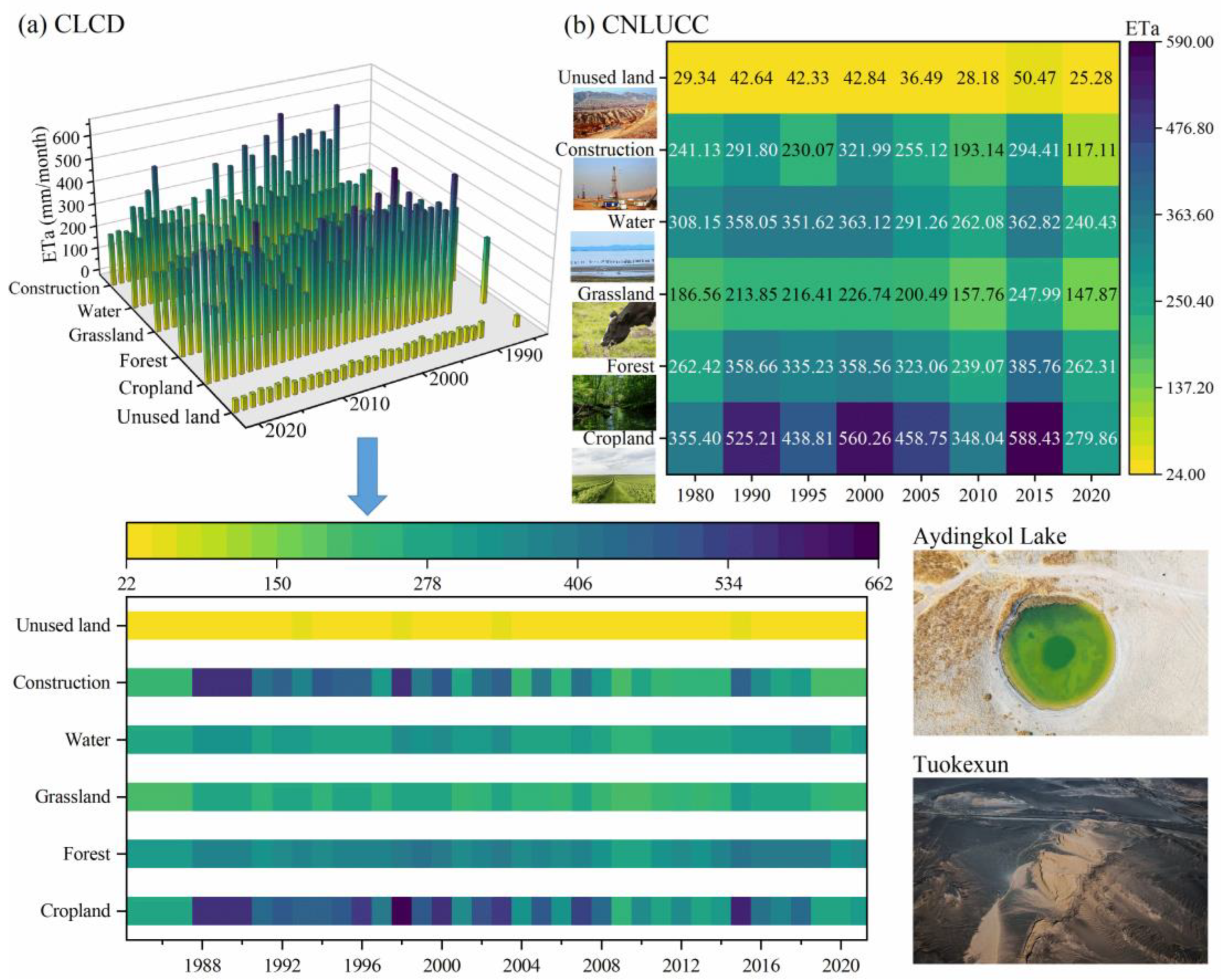
  • The differences in the physicochemical properties of different land classes determine the disparities in their ETa capacities. As shown in Figure 19, the annual average ETa of cropland in Tuha was the highest, reaching 424.12 mm/a, indicating that cropland has higher water-use efficiency and ET potential. The annual average ETa of unused land was the lowest, at only 32.27 mm/a, reflecting the low vegetation coverage and weak evaporation capacity of unused land. The annual average ETa values of the forest, construction land, water, and grassland were between these two values.
  • The urban heat-island effect has a certain impact on the ETa of construction and unused land. The land-surface temperatures of these two types of land were higher than those of other land types, especially in the summer. Since TEM is one of the important factors affecting the ET process, the ETa values of these two land types likewise fluctuated with TEM; nevertheless, their ETa values remained lower because bare soil acts as a suppressor of water evaporation [66].
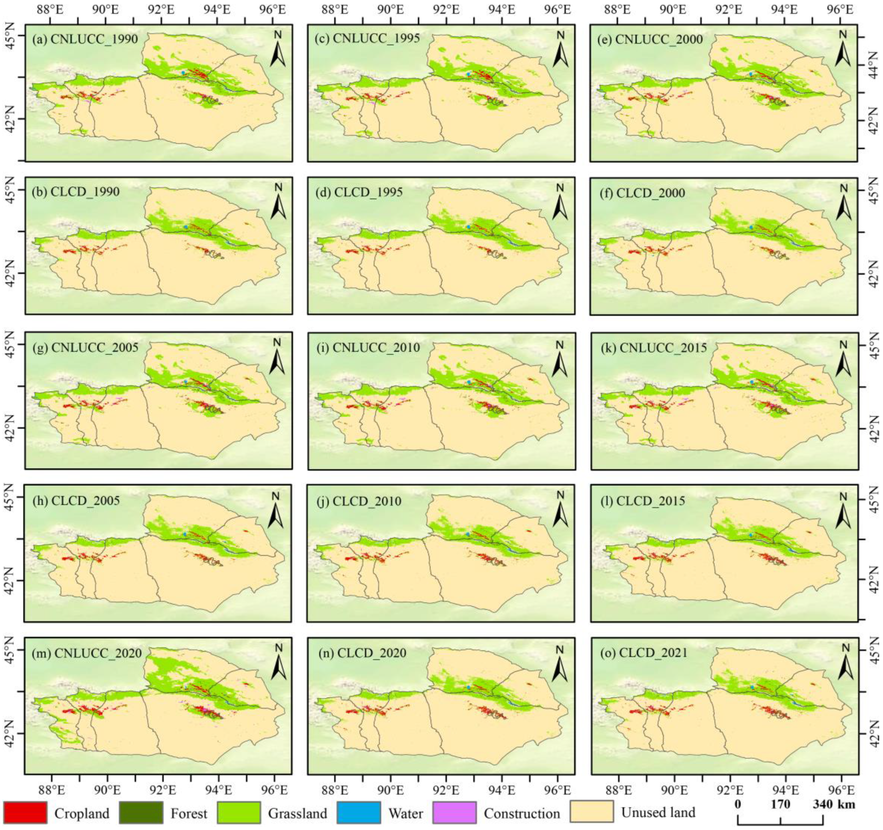
  • LUCC has a significant effect on Tuha’s ETa. During 1980–2021, significant land-use changes occurred in Tuha, and this led to corresponding changes in the ETa values for different land types. Except for the forest, the annual average ETa values of the other five types of land showed downward trends, indicating an overall decrease in the ETa capacity of Tuha.

4. Discussion

The Turpan–Hami region, as an important part of the northwest arid area, is sensitive to climate change. Therefore, this study compares the actual evapotranspiration characteristics of the Turpan–Hami region with those of the northwest arid region. Deng et al. found that the spatial distribution of ETa in the northwest arid region is influenced by both PRCP and LUCC [67]. Due to its inland location and low PRCP, the area of low ETa is large. The leeward slopes of high mountains such as the Qilian mountains and Tianshan mountains have abundant PRCP, while the surrounding basin and corridor have low PRCP. Therefore, the amount of ETa gradually decreases from the mountainous areas to the plains on both sides, which is consistent with the distribution shown in Figure 7a. Ji et al. used 12 grassland flux stations and satellite remote sensing products to produce a 5 km ETa product and found that from 2000 to 2018, the non-bare ground underlying surface in the northwest showed an overall increasing trend of ETa (19 mm/a) [68], which is consistent with the results shown in Figure 13c of this study, indicating an increase in ETa in the mountain forests and grasslands where PRCP is abundant. Wei et al. predicted the ETa data of China’s PML-V2 from 2003 to 2020 and found that most of the Hurst indices in the Turpan–Hami region were less than 0.5, indicating that the future trend is opposite to the past [19]. This is consistent with the results shown in Figure 15a of this article. At the same time, due to differences in dynamic and thermodynamic properties, the difference in ETa between different land cover types is significant. Kong et al. found that from 2000 to 2018, the average ETa of different land uses in the Manas River Basin ranked from large to small: forest (418.65 mm) > water (302.36 mm) > cropland (257.32 mm) > unused land (222.00 mm) > construction land (218.10 mm) > grassland (207.04 mm) [69]. Deng et al. found that the forest had the largest amount of ETa [67], while the results in this study were arranged in the order of cropland > forest > grassland > unused land, mainly due to the smaller areas of forests and water bodies in the study area. Fu et al. analyzed the spatiotemporal variation characteristics of ETa on land in China from 2000 to 2019 using a model–process–mechanism framework and concluded that PRCP is the main factor determining the size of ETa in the northwest arid zone [64]. The findings of Fu et al.’s study are similar to those of the present study. Therefore, our findings add new evidence to the understanding of ETa patterns in different spatial dimensions in the Turpan–Hami region.
Under the combined influence of human activities and climate change, ETa saw a weakly decreasing trend in most regions of Tuha from 1980 to 2021, with a change rate of −0.2 mm/a, and the trend was dominated by large fluctuations. The typical oasis agriculture that has developed in Tuha, the implementation of the project for returning farmland to forest and grassland, the expansion of oasis areas, the adjustment of planting structures, and changes in the species that are planted will cause fluctuations in ETa. In addition to human activities, climate change is also having a profound impact on the variation of ETa, especially in the alpine mountains with their fragile ecological environment. The response of ETa to climate change and the time-series variation of ETa in China have been extensively discussed [70,71,72]. The natural elements of the Tuha “mountain–oasis–desert” system have distinctive characteristics and are highly representative of arid zones. This study’s findings provide a scientific reference for understanding the spatial and temporal ET patterns in arid regions driven by global warming and human activities.
It is predicted that the future of ETa in Tuha will have a significant anti-continuous trend, i.e., ETa in most of Tuha will be anti-continuously increasing in the future. The high Hurst values were found to be mainly concentrated in the junction zone of Balikunhasake and southern Yiwu, and low Hurst values were more widely distributed, mainly across Turpan City, northwestern Balikunhasake, and southeastern Yizhou. This trend of an anti-continuous increase in variability will affect the special ecological and environmental elements of the arid zone, such as oases, dust storms, and lakes. The questions of whether the trend of increasing ETa will continue to develop with changes in the regional climate system and anthropogenic interventions, and how the hydrological cycle, ecosystems, and surface processes in the arid zone will respond [73]—especially regarding the impact of conservation and restoration of the desert ecosystem—will require comprehensive and longitudinal data and an in-depth study to answer.

5. Conclusions

In this work, we quantitatively estimated the monthly ETa of Tuha at a 1 km resolution from 1980 to 2021 using the ETMonitor model based on multi-source RS and reanalysis data. We then analyzed the spatiotemporal characteristics of the pixel-scale ETa of Tuha over the past 42 years using Sen, MK, CV, and Hurst. Finally, we explored the correlations between ETa, TEM, and PRCP in Tuha and the spatial ETa distribution characteristics and trends of different land types. The main conclusions of this work are as follows.
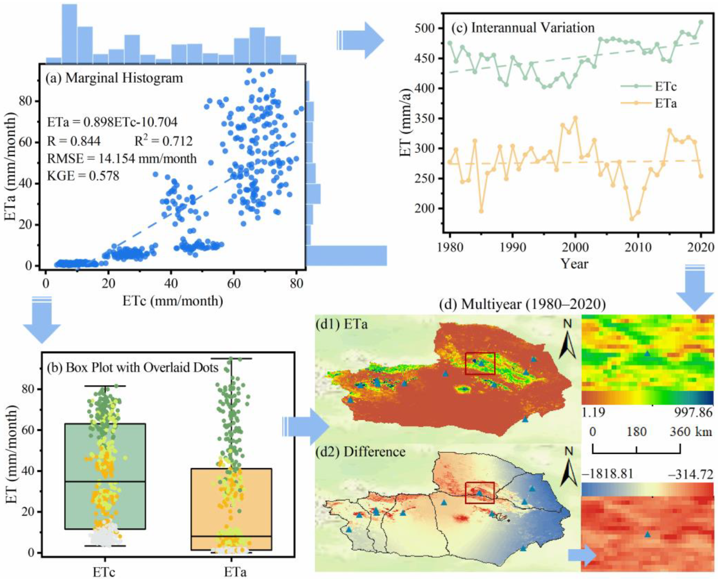
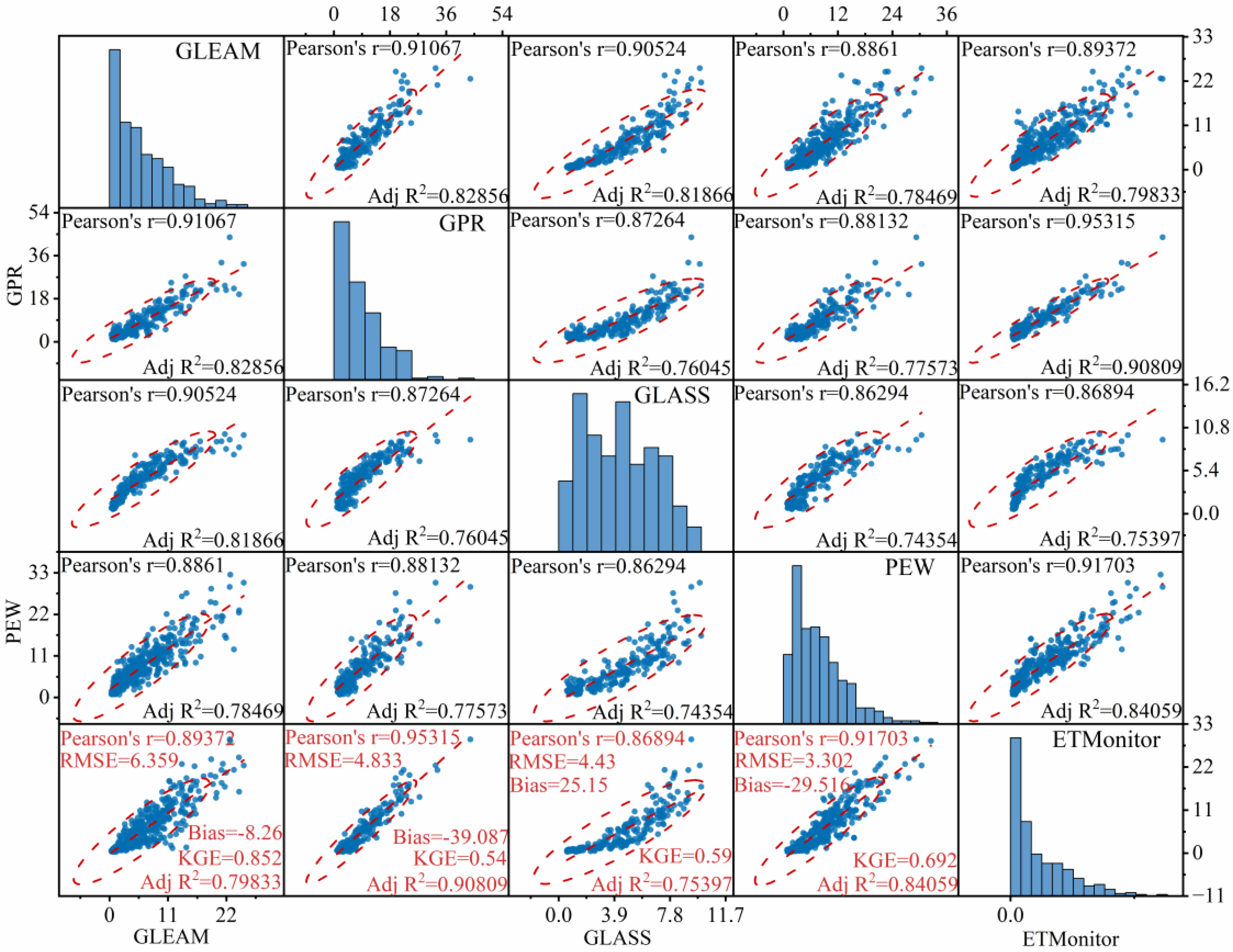
  • The R between the estimated results of this study and the PM calculation results and existing ETa products such as PEW are all greater than 0.8, the corresponding R2 values are between 0.7 and 0.9, and the RMSE values are all less than 15 mm/month. This verifies that the results of the ETMonitor model in Tuha inversion have high reliability and can be used to analyze the spatial and temporal variation characteristics of Tuha’s ETa.
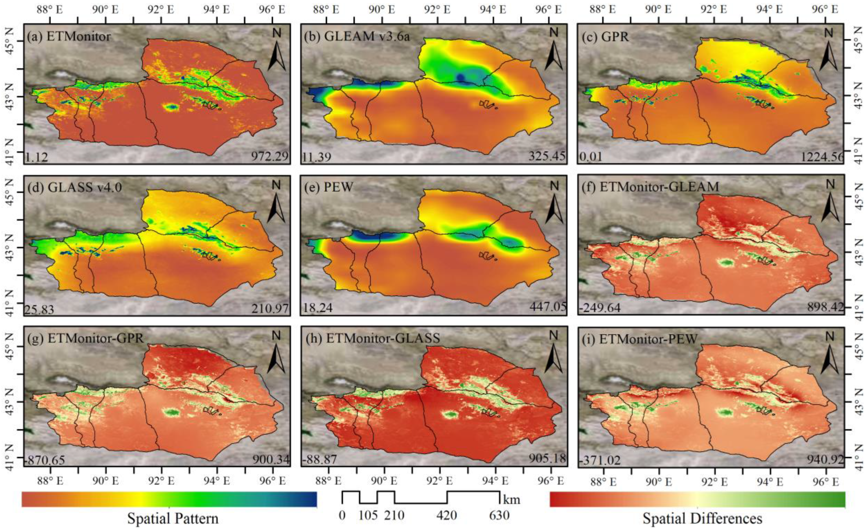
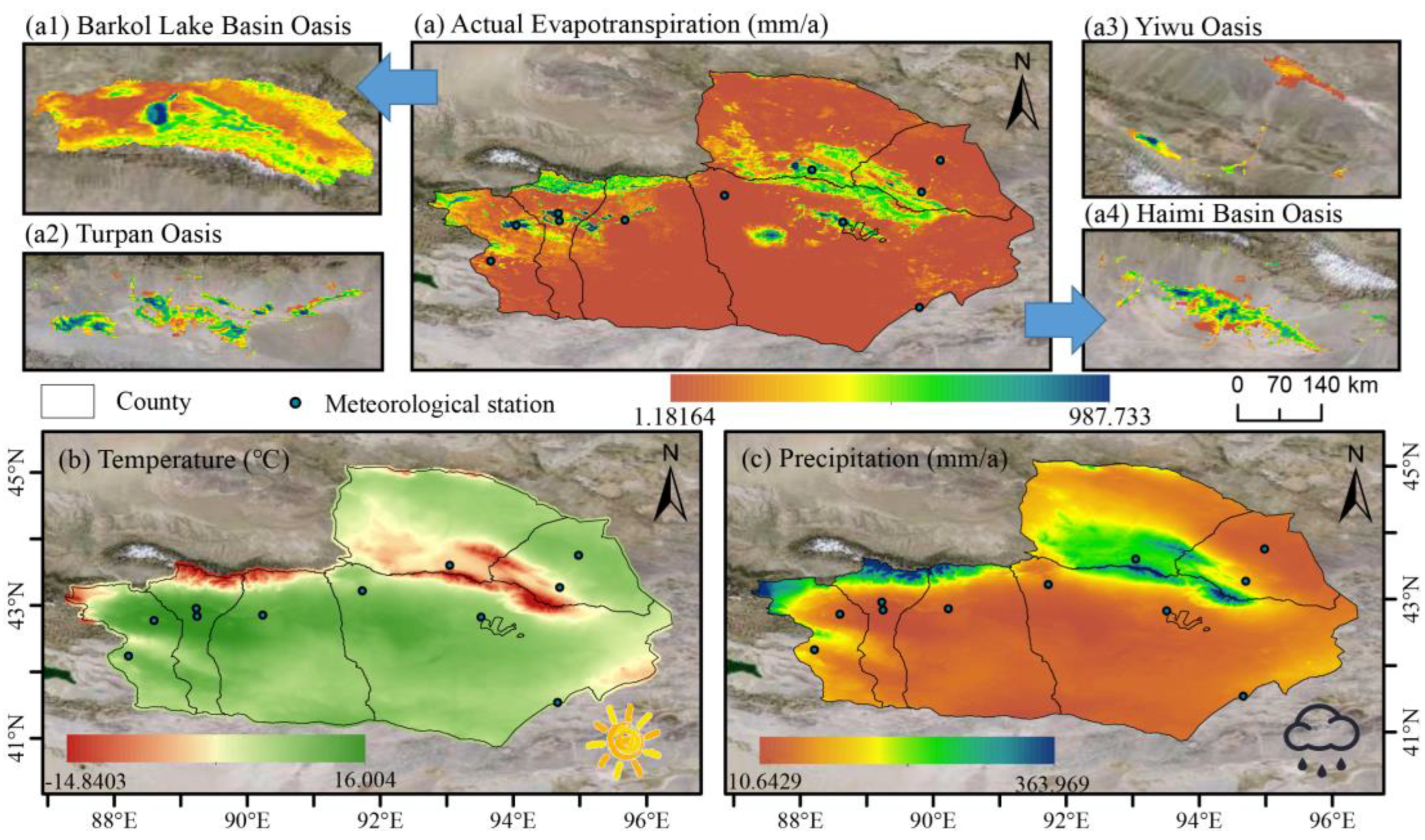
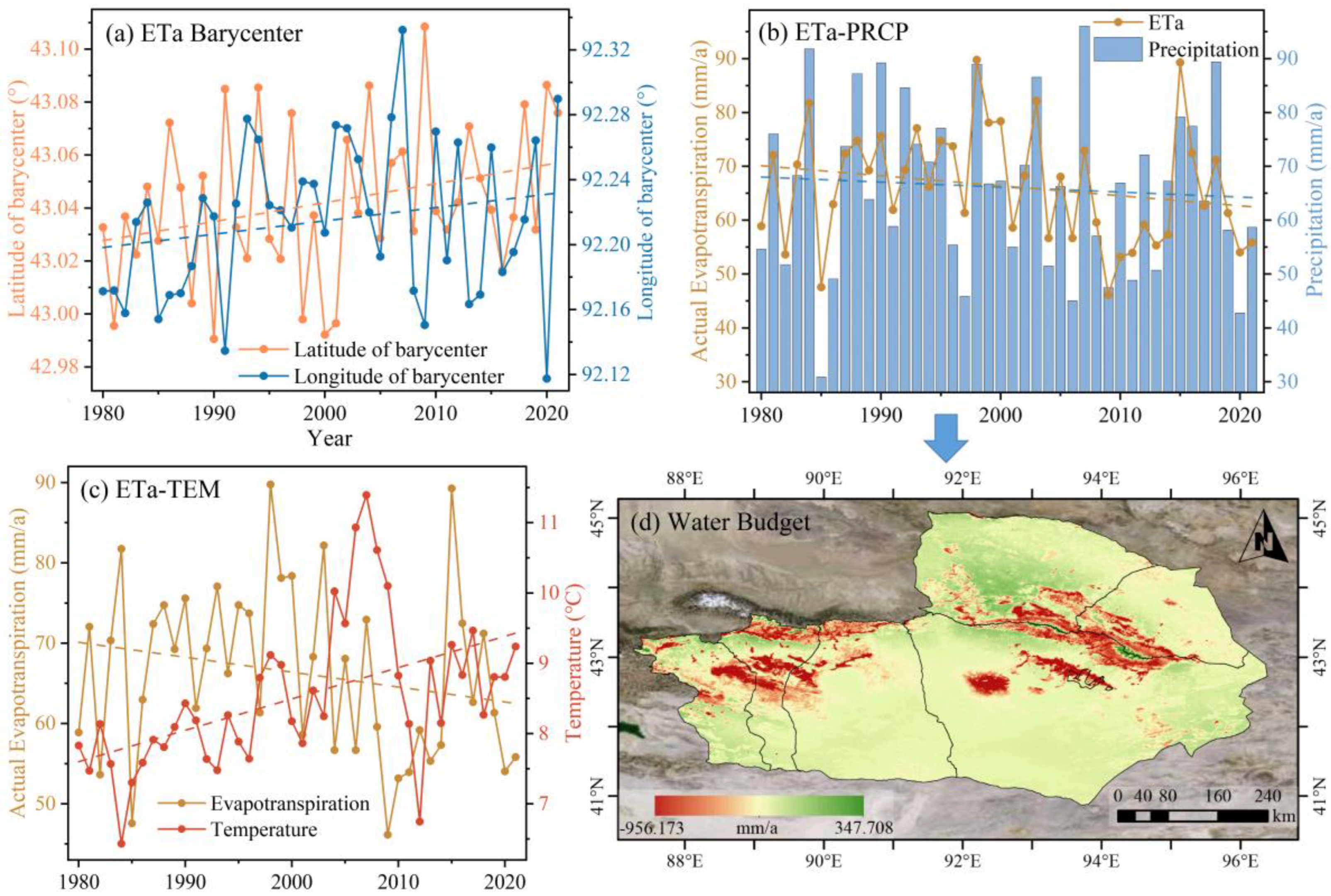
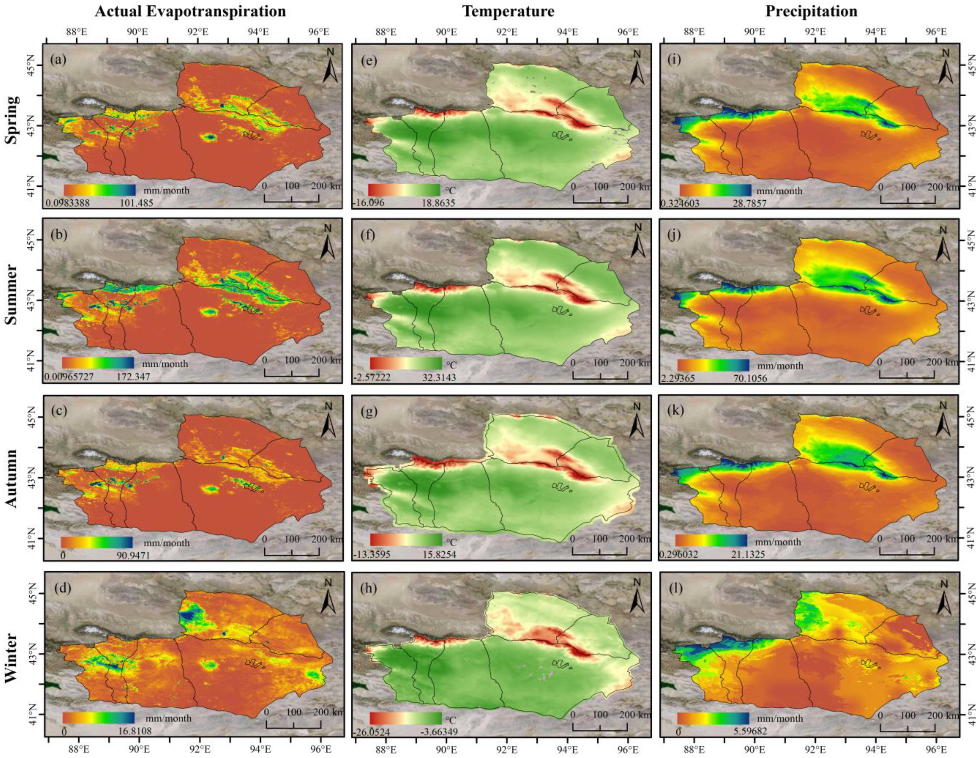
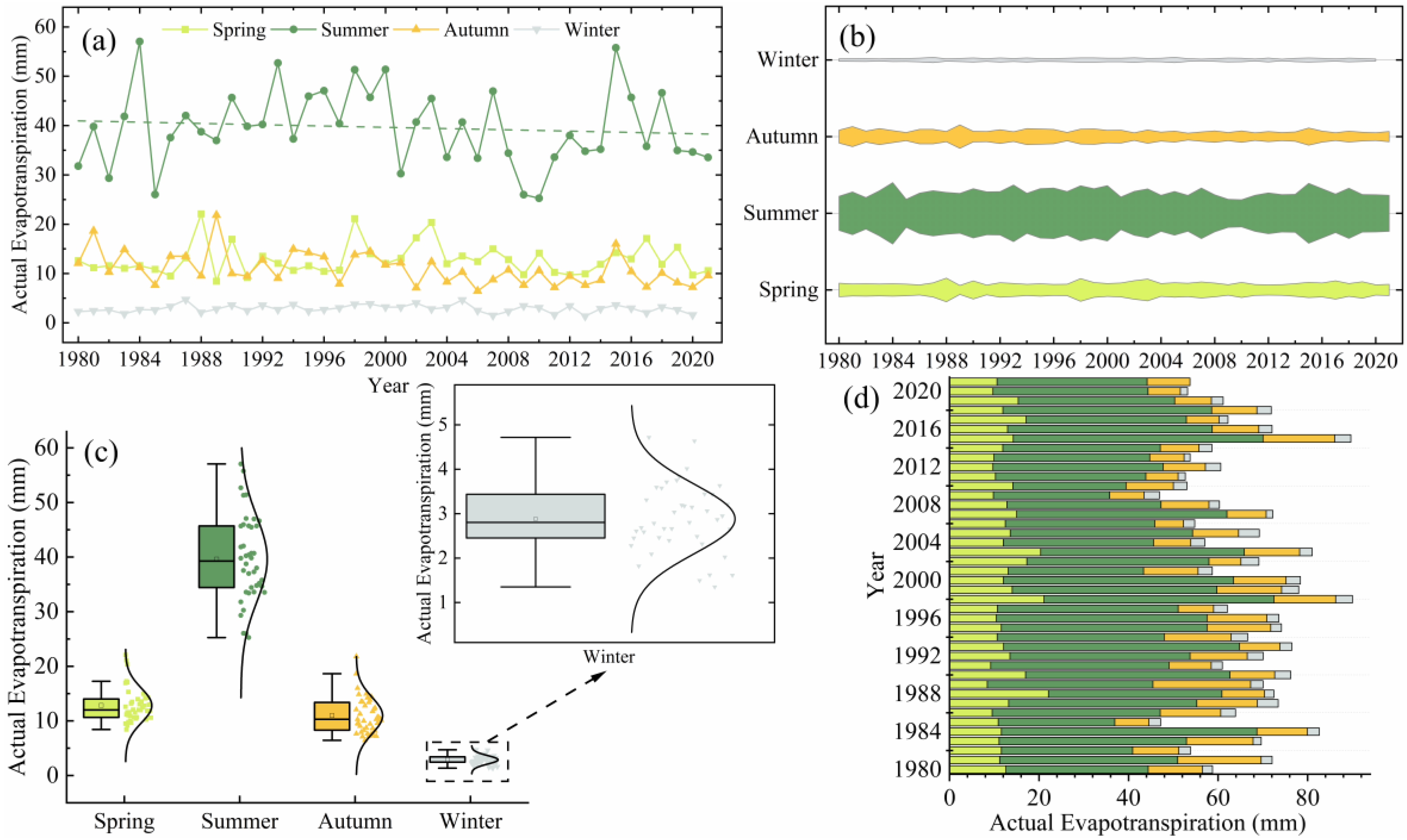
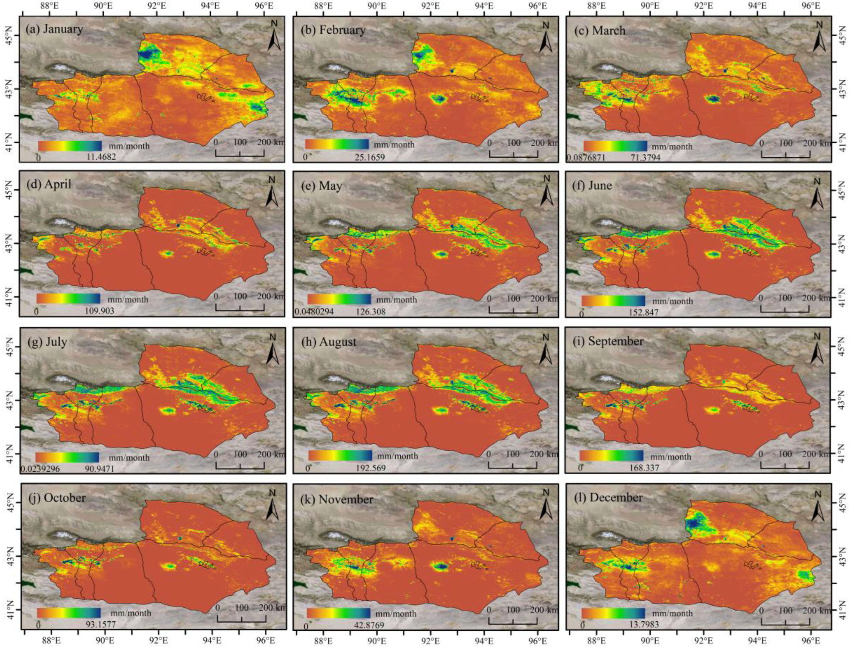
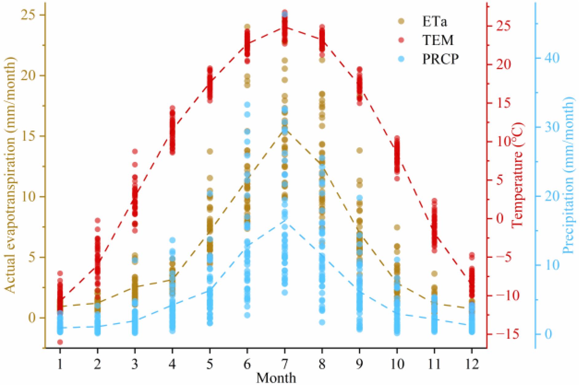
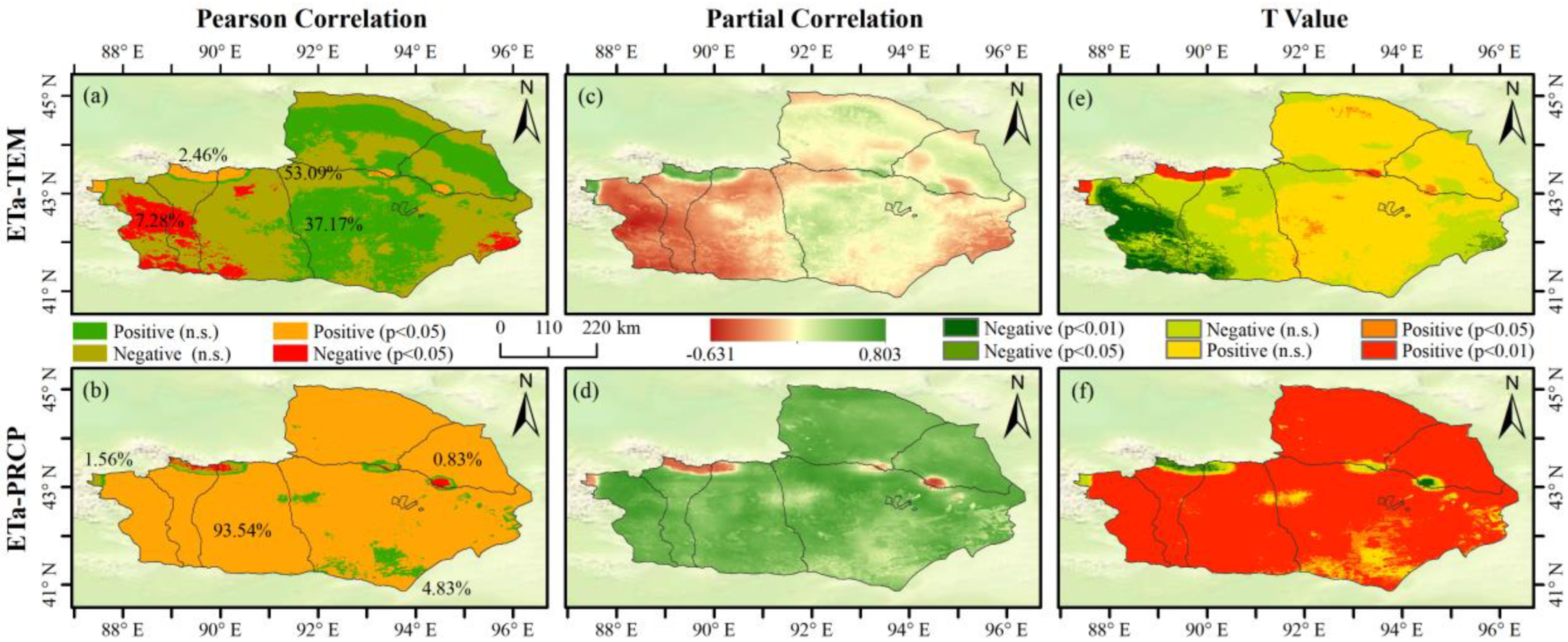
  • There are significant regional differences and seasonal variations in the spatial distribution of Tuha’s ETa. The high values are mainly located in mountainous valley areas with high PRCP and in plain areas adjacent to rivers and water supply zones; this is similar to the spatial patterns of LUCC and PRCP. The trend of annual ETa in each pixel was mainly dominated by the trend of ETa in summer; the influences of spring, autumn, and winter on the trend of annual ETa were weak. The overall interannual changes in ETa in Tuha from 1980 to 2021 showed a fluctuating decreasing trend; the monthly ETa showed a single-peaked curve, which was basically consistent with the characteristics of the monthly TEM and PRCP changes. This indicates that the changes in Tuha’s ETa were closely related to the changes in hydrothermal conditions, especially maintaining a correlation with water changes. A similar pattern was shown on the pixel scale: ETa and PRCP were mainly significantly and positively correlated, while there was a non-significant positive correlation with TEM.
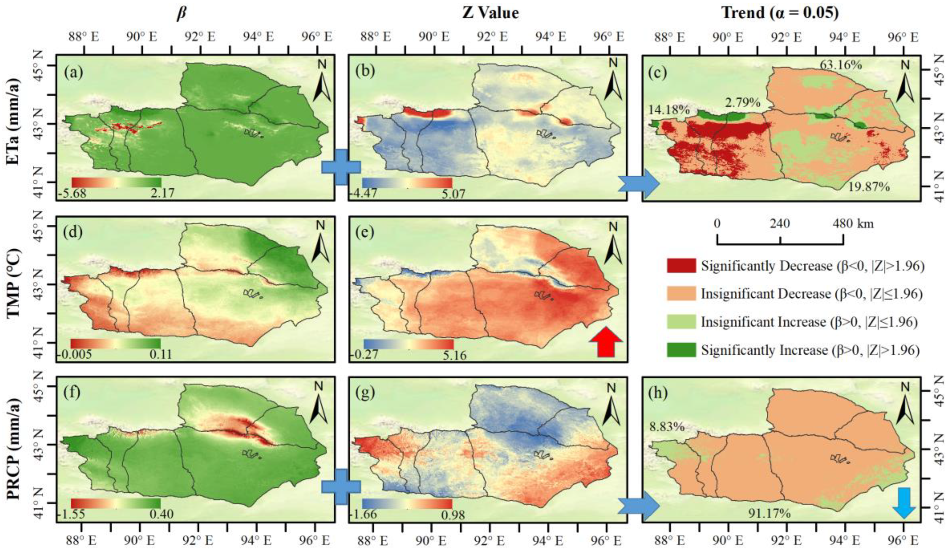
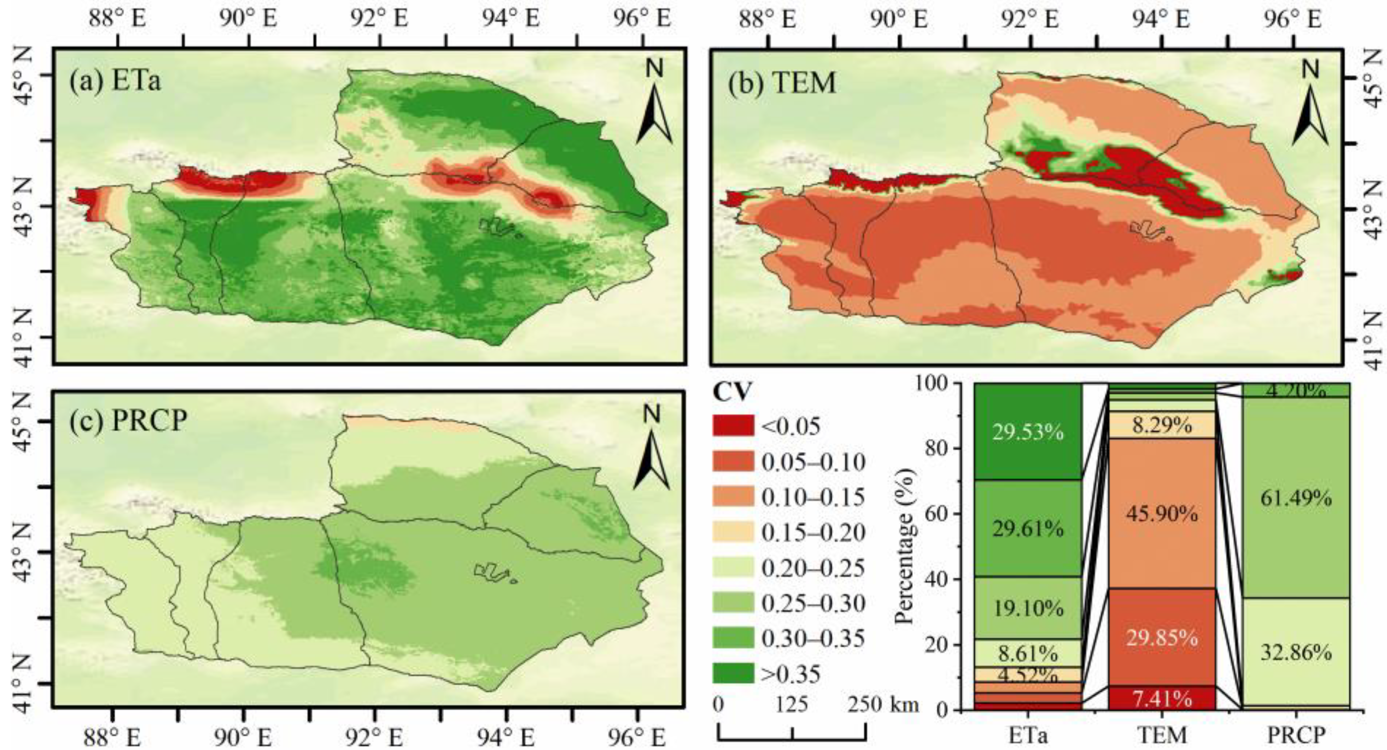
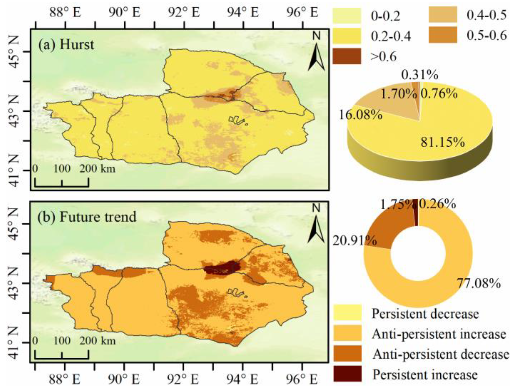
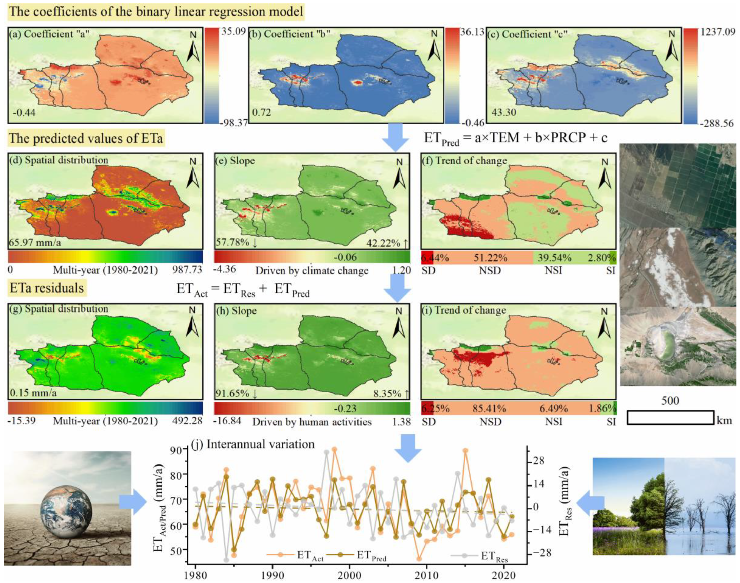
  • The trend rate of change of ETa in Tuha from 1980 to 2021 ranged from −16.78 to 2.17 mm/a, with an average trend rate of change of −0.2 mm/a, showing an overall decreasing trend. Spatially, there was an increase around the mountain range, the southwestern part of Yizhou, the northern part of Balikunhasake and Yiwu, and there was a decrease in the southern part of Turpan City. The areas of high ETa fluctuation were mainly concentrated in the south of Tuha and the northeast of Balikunhasake and Yiwu, and the land types in these areas were mainly bare land; the huge ETa fluctuations here could be due to the implementation of the ecological restoration project (returning cropland to forest and grass) in Tuha and the increase in urbanization. The ETa evolution trends were all significantly resistant to persistence, and 78.23% of the areas were predicted to have increases in ETa.
  • The anthropogenic impact in the Turpan–Hami region exhibited a slight decreasing trend (85.41%), with 91.65% of the area experiencing an increase while only 8.35% showing a decrease in human impact. The ETa intensities of different land-use types in Tuha differed significantly: cropland (424.12 mm/a) > forest (354.65 mm/a) > construction (324.9 mm/a) > water (301.45 mm/a) > grassland (241.39 mm/a) > unused land (32.27 mm/a). During the study period, the average annual ETa values of cropland, grassland, water, construction, and unused land showed decreasing trends; the forest showed a roughly stable and constant trend, and the changes in land-use type also affected the changes in ETa.

Author Contributions

L.W.: conceptualization, methodology, software, visualization, and writing—original draft; J.W.: methodology, software, supervision, project administration, and writing—review and editing; J.D.: resources, supervision, and funding acquisition; X.L.: conceptualization, methodology, validation, and software. All authors have read and agreed to the published version of the manuscript.

Funding

This study was supported by the Basic Resources Investigation Project of the Ministry of Science and Technology: Water Resources Investigation and carrying capacity assessment of Turpan–Hami Basin (2021xjkk1000).

Data Availability Statement

All data used in this study can be accessed from the websites as follows: GLASS v4.0 (http://www.glass.umd.edu, URL (accessed on 25 March 2023) and http://www.geodata.cn/thematicView/GLASS.html, URL (accessed on 25 March 2023)); MODIS (https://search.earthdata.nasa.gov, URL (accessed on 25 March 2023)); ESA CCI v07.1 (https://esa–soilmoisture–cci.org, URL (accessed on 25 March 2023)); ERA5 (https://www.ecmwf.int/en/forecasts/datasets/reanalysis–datasets/era5, URL (accessed on 25 March 2023)); LUCC (https://zenodo.org/record/5816591 and http://www.resdc.cn, URL (accessed on 25 March 2023)); Soil Hydraulic Properties (https://dataverse.harvard.edu/dataset.xhtml?persistentId=doi:10.7910/DVN/UI5LCE, URL (accessed on 25 March 2023)); GLEAM v3.6a (https://www.gleam.eu/, URL (accessed on 25 March 2023)); PEW, SM, TEM, and PRCP (https://data.tpdc.ac.cn/, URL (accessed on 25 March 2023)). The code for analyzing the spatiotemporal evolution and attribution of actual evapotranspiration in the Turpan–Hami region has been shared at https://mp.weixin.qq.com/s/0irvPqXYO036ZYxu77r9Yg, URL (accessed on 20 April 2023).

Acknowledgments

We are sincerely grateful to the reviewers and editors for their constructive comments on the improvement of the manuscript.

Conflicts of Interest

The authors declare no conflict of interest.

References

  1. Mai, M.; Wang, T.; Han, Q.; Jing, W.; Bai, Q. Comparison of environmental controls on daily actual evapotranspiration dynamics among different terrestrial ecosystems in China. Sci. Total Environ. 2023, 871, 162124. [Google Scholar] [CrossRef]
  2. Wu, B.; Quan, Q.; Yang, S.; Dong, Y. A social-ecological coupling model for evaluating the human-water relationship in basins within the Budyko framework. J. Hydrol. 2023, 619, 129361. [Google Scholar] [CrossRef]
  3. Zhao, M.; Geruo, A.G.; Liu, Y.; Konings, A.G. Evapotranspiration frequently increases during droughts. Nat. Clim. Chang. 2022, 12, 1024–1030. [Google Scholar] [CrossRef]
  4. Mustafa, A.; Alam, I.M.; Najah, A.A.; Feng, H.Y. A novel application of transformer neural network (TNN) for estimating pan evaporation rate. Appl. Water Sci. 2022, 13, 31. [Google Scholar] [CrossRef]
  5. Mokhtari, A.; Sadeghi, M.; Afrasiabian, Y.; Yu, K. OPTRAM-ET: A novel approach to remote sensing of actual evapotranspiration applied to Sentinel-2 and Landsat-8 observations. Remote Sens. Environ. 2023, 286, 113443. [Google Scholar] [CrossRef]
  6. Shang, K.; Yao, Y.; Di, Z.; Jia, K.; Zhang, X.; Fisher, J.B.; Chen, J.; Guo, X.; Yang, J.; Yu, R.; et al. Coupling physical constraints with machine learning for satellite-derived evapotranspiration of the Tibetan Plateau. Remote Sens. Environ. 2023, 289, 113519. [Google Scholar] [CrossRef]
  7. Song, L.; Ding, Z.; Kustas, W.P.; Xu, Y.; Zhao, G.; Liu, S.; Ma, M.; Xue, K.; Bai, Y.; Xu, Z. Applications of a thermal-based two-source energy balance model coupled to surface soil moisture. Remote Sens. Environ. 2022, 271, 112923. [Google Scholar] [CrossRef]
  8. Yang, J.; Yao, Y.; Shao, C.; Li, Y.; Fisher, J.B.; Cheng, J.; Chen, J.; Jia, K.; Zhang, X.; Shang, K.; et al. A novel TIR-derived three-source energy balance model for estimating daily latent heat flux in mainland China using an all-weather land surface Temperature product. Agric. For. Meteorol. 2022, 323, 109066. [Google Scholar] [CrossRef]
  9. Wei, J.; Cui, Y.; Luo, Y. Rice growth period detection and paddy field evapotranspiration estimation based on an improved SEBAL model: Considering the applicable conditions of the advection equation. Agric. Water Manag. 2023, 278, 108141. [Google Scholar] [CrossRef]
  10. Zhang, C.; Long, D.; Zhang, Y.; Anderson, M.C.; Kustas, W.P.; Yang, Y. A decadal (2008–2017) daily evapotranspiration data set of 1 km spatial resolution and spatial completeness across the North China Plain using TSEB and data fusion. Remote Sens. Environ. 2021, 262, 112519. [Google Scholar] [CrossRef]
  11. Jaafar, H.; Mourad, R.; Schull, M. A global 30-m ET model (HSEB) using harmonized Landsat and Sentinel-2, MODIS and VIIRS: Comparison to ECOSTRESS ET and LST. Remote Sens. Environ. 2022, 274, 112995. [Google Scholar] [CrossRef]
  12. Zou, M.; Yang, K.; Lu, H.; Ren, Y.; Sun, J.; Wang, H.; Tan, S.; Zhao, L. Integrating eco-evolutionary optimality principle and land processes for evapotranspiration estimation. J. Hydrol. 2023, 616, 128855. [Google Scholar] [CrossRef]
  13. Zheng, C.; Jia, L.; Hu, G. Global land surface evapotranspiration monitoring by ETMonitor model driven by multi-source satellite earth observations. J. Hydrol. 2022, 613, 128444. [Google Scholar] [CrossRef]
  14. Hu, G.; Jia, L. Monitoring of Evapotranspiration in a Semi-Arid Inland River Basin by Combining Microwave and Optical Remote Sensing Observations. Remote Sens. 2015, 7, 3056–3087. [Google Scholar] [CrossRef]
  15. Paciolla, N.; Corbari, C.; Hu, G.; Zheng, C.; Menenti, M.; Jia, L.; Mancini, M. Evapotranspiration estimates from an energy-water-balance model calibrated on satellite land surface Temperature over the Heihe basin. J. Arid. Environ. 2021, 188, 104466. [Google Scholar] [CrossRef]
  16. Abbasi, N.; Nouri, H.; Didan, K.; Barreto-Muñoz, A.; Chavoshi Borujeni, S.; Opp, C.; Nagler, P.; Thenkabail, P.S.; Siebert, S. Mapping Vegetation Index-Derived Actual Evapotranspiration across Croplands Using the Google Earth Engine Platform. Remote Sens. 2023, 15, 1017. [Google Scholar] [CrossRef]
  17. Senay, G.B.; Friedrichs, M.; Morton, C.; Parrish, G.E.L.; Schauer, M.; Khand, K.; Kagone, S.; Boiko, O.; Huntington, J. Mapping actual evapotranspiration using Landsat for the conterminous United States: Google Earth Engine implementation and assessment of the SSEBop model. Remote Sens. Environ. 2022, 275, 113011. [Google Scholar] [CrossRef]
  18. Degano, M.F.; Rivas, R.E.; Carmona, F.; Niclòs, R.; Sánchez, J.M. Evaluation of the MOD16A2 evapotranspiration product in an agricultural area of Argentina, the Pampas region. Egypt. J. Remote Sens. Space Sci. 2021, 24, 319–328. [Google Scholar] [CrossRef]
  19. Wei, T.; Wang, Y.Q. Temporal and spatial dynamic analysis of terrestrial evapotranspiration in China based on PML-V2 product. Arid. Land Geogr. 2023, 1–15. [Google Scholar]
  20. Deng, H.; Tang, Q.; Yun, X.; Tang, Y.; Liu, X.; Xu, X.; Sun, S.; Zhao, G.; Zhang, Y.; Zhang, Y. Wetting trend in Northwest China reversed by warmer Temperature and drier air. J. Hydrol. 2022, 613, 128435. [Google Scholar] [CrossRef]
  21. Condon, L.E.; Atchley, A.L.; Maxwell, R.M. Evapotranspiration depletes groundwater under warming over the contiguous United States. Nat. Commun. 2020, 11, 873. [Google Scholar] [CrossRef] [PubMed]
  22. Wang, Y.; Feng, G.; Li, Z.; Luo, S.; Wang, H.; Xiong, Z.; Zhu, J.; Hu, J. A Strategy for Variable-Scale InSAR Deformation Monitoring in a Wide Area: A Case Study in the Turpan–Hami Basin, China. Remote Sens. 2022, 14, 3832. [Google Scholar] [CrossRef]
  23. Yan, N.; Wu, B.; Zhu, W. Assessment of Agricultural Water Productivity in Arid China. Water 2020, 12, 1161. [Google Scholar] [CrossRef]
  24. Zhang, M.; Philp, P. Geochemical characterization of aromatic hydrocarbons in crude oils from the Tarim, Qaidam and Turpan Basins, NW China. Pet. Sci. 2010, 7, 448–457. [Google Scholar] [CrossRef]
  25. Liu, N.F.; Liu, Q.; Wang, L.Z.; Liang, S.L.; Wen, J.G.; Qu, Y.; Liu, S.H. A statistics-based temporal filter algorithm to map spatiotemporally continuous shortwave albedo from MODIS data. Hydrol. Earth Syst. Sci. 2013, 17, 2121–2129. [Google Scholar] [CrossRef]
  26. Liu, Q.; Wang, L.; Qu, Y.; Liu, N.; Liu, S.; Tang, H.; Liang, S. Preliminary evaluation of the long-term GLASS albedo product. Int. J. Digit. Earth 2013, 6, 69–95. [Google Scholar] [CrossRef]
  27. Xiao, Z.; Liang, S.; Wang, J.; Chen, P.; Yin, X.; Zhang, L.; Song, J. Use of General Regression Neural Networks for Generating the GLASS Leaf Area Index Product From Time-Series MODIS Surface Reflectance. IEEE Trans. Geosci. Remote Sens. 2014, 52, 209–223. [Google Scholar] [CrossRef]
  28. Jia, K.; Liang, S.; Liu, S.; Li, Y.; Xiao, Z.; Yao, Y.; Jiang, B.; Zhao, X.; Wang, X.; Xu, S.; et al. Global Land Surface Fractional Vegetation Cover Estimation Using General Regression Neural Networks from MODIS Surface Reflectance. IEEE Trans. Geosci. Remote Sens. 2015, 53, 4787–4796. [Google Scholar] [CrossRef]
  29. Sulla-Menashe, D.; Gray, J.M.; Abercrombie, S.P.; Friedl, M.A. Hierarchical mapping of annual global land cover 2001 to present: The MODIS Collection 6 Land Cover product. Remote Sens. Environ. 2019, 222, 183–194. [Google Scholar] [CrossRef]
  30. Yang, J.; Huang, X. The 30 m annual land cover dataset and its dynamics in China from 1990 to 2019. Earth Syst. Sci. Data 2021, 13, 3907–3925. [Google Scholar] [CrossRef]
  31. Xu, X.L.; Liu, J.Y.; Zhang, S.W.; Li, R.D.; Yan, C.Z.; Wu, S.X. Multi-period land use remote sensing data set in China (CNLUCC). Resour. Environ. Sci. Data Regist. Publ. Syst. 2018, 7, 201. [Google Scholar]
  32. Gruber, A.; Scanlon, T.; van der Schalie, R.; Wagner, W.; Dorigo, W. Evolution of the ESA CCI Soil Moisture climate data records and their underlying merging methodology. Earth Syst. Sci. Data 2019, 11, 717–739. [Google Scholar] [CrossRef]
  33. Martens, B.; Miralles, D.G.; Lievens, H.; van der Schalie, R.; de Jeu, R.A.M.; Fernández-Prieto, D.; Beck, H.E.; Dorigo, W.A.; Verhoest, N.E.C. GLEAM v3: Satellite-based land evaporation and root-zone soil moisture. Geosci. Model Dev. 2017, 10, 1903–1925. [Google Scholar] [CrossRef]
  34. Jianyu, F.; Weiguang, W.; Quanxi, S.; Wanqiu, X.; Mingzhu, C.; Jia, W.; Zefeng, C.; Wanshu, N. Improved global evapotranspiration estimates using proportionality hypothesis-based water balance constraints. Remote Sens. Environ. 2022, 279, 113140. [Google Scholar] [CrossRef]
  35. Yao, Y.; Liang, S.; Li, X.; Hong, Y.; Fisher, J.B.; Zhang, N.; Chen, J.; Cheng, J.; Zhao, S.; Zhang, X.; et al. Bayesian multimodel estimation of global terrestrial latent heat flux from eddy covariance, meteorological, and satellite observations. J. Geophys. Res. Atmos. 2014, 119, 4521–4545. [Google Scholar] [CrossRef]
  36. Yao, Y.; Liang, S.; Cheng, J.; Liu, S.; Fisher, J.B.; Zhang, X.; Jia, K.; Zhao, X.; Qin, Q.; Zhao, B.; et al. MODIS-driven estimation of terrestrial latent heat flux in China based on a modified Priestley–Taylor algorithm. Agric. For. Meteorol. 2013, 171–172, 187–202. [Google Scholar] [CrossRef]
  37. Yin, L.; Tao, F.; Chen, Y.; Liu, F.; Hu, J. Improving terrestrial evapotranspiration estimation across China during 2000–2018 with machine learning methods. J. Hydrol. 2021, 600, 126538. [Google Scholar] [CrossRef]
  38. Li, Z.; Sang, X.; Zhang, S.; Zheng, Y.; Lei, Q. Conversion Coefficient Analysis and Evaporation Dataset Reconstruction for Two Typical Evaporation Pan Types—A Study in the Yangtze River Basin, China. Atmosphere 2022, 13, 1322. [Google Scholar] [CrossRef]
  39. Allen, R.G.; Pereira, L.S.; Raes, D.; Smith, M. Crop Evapotranspiration. Guidelines for Computing Crop Water Requirements; FAO Irrigation and Drainage Paper; Food and Agriculture Organization: Rome, Italy, 1998; p. 56. [Google Scholar]
  40. Binbin, G.; Jing, Z.; Xianyong, M.; Tingbao, X.; Yongyu, S. Long-term spatio-temporal precipitation variations in China with precipitation surface interpolated by ANUSPLIN. Sci. Rep. 2020, 10, 81. [Google Scholar] [CrossRef]
  41. Peng, S.; Ding, Y.; Liu, W.; Li, Z. 1 km monthly Temperature and precipitation dataset for China from 1901 to 2017. Earth Syst. Sci. Data 2019, 11, 1931–1946. [Google Scholar] [CrossRef]
  42. Peng, S.; Gang, C.; Cao, Y.; Chen, Y. Assessment of climate change trends over the Loess Plateau in China from 1901 to 2100. Int. J. Climatol. 2018, 38, 2250–2264. [Google Scholar] [CrossRef]
  43. Peng, S.; Ding, Y.; Wen, Z.; Chen, Y.; Cao, Y.; Ren, J. Spatiotemporal change and trend analysis of potential evapotranspiration over the Loess Plateau of China during 2011–2100. Agric. For. Meteorol. 2017, 233, 183–194. [Google Scholar] [CrossRef]
  44. Suling, H.; Jie, L.; Jinliang, W.; Fang, L. Evaluation and analysis of upscaling of different land use/land cover products (FORM-GLC30, GLC_FCS30, CCI_LC, MCD12Q1 and CNLUCC): A case study in China. Geocarto Int. 2022, 37, 17340–17360. [Google Scholar] [CrossRef]
  45. Zheng, C.; Jia, L.; Hu, G.; Lu, J. Earth Observations-Based Evapotranspiration in Northeastern Thailand. Remote Sens. 2019, 11, 138. [Google Scholar] [CrossRef]
  46. Zhang, Y.; Schaap, M.G.; Zha, Y. A High-Resolution Global Map of Soil Hydraulic Properties Produced by a Hierarchical Parameterization of a Physically Based Water Retention Model. Water Resour. Res. 2018, 54, 9774–9790. [Google Scholar] [CrossRef]
  47. Ning, W.; Li, J.; Chaolei, Z.; Massimo, M. Estimation of subpixel snow sublimation from multispectral satellite observations. J. Appl. Remote Sens. 2017, 11, 46017. [Google Scholar] [CrossRef]
  48. Allen, R.G.; Pruitt, W.O.; Wright, J.L.; Howell, T.A.; Ventura, F.; Snyder, R.; Itenfisu, D.; Steduto, P.; Berengena, J.; Yrisarry, J.B.; et al. A recommendation on standardized surface resistance for hourly calculation of reference ETo by the FAO56 Penman-Monteith method. Agric. Water Manag. 2006, 81, 1–22. [Google Scholar] [CrossRef]
  49. Noilhan, J.; Planton, S. A Simple Parameterization of Land Surface Processes for Meteorological Models. Am. Meteorol. Soc. 1989, 117, 536–549. [Google Scholar] [CrossRef]
  50. Shuttleworth, W.J.; Wallace, J.S. Evaporation from sparse crops-an energy combination theory. Q. J. R. Meteorol. Soc. 1985, 111, 839–855. [Google Scholar] [CrossRef]
  51. Song, P.; Zhang, Y.; Guo, J.; Shi, J.; Zhao, T.; Tong, B. A 1-km daily surface soil moisture dataset of enhanced coverage under all-weather conditions over China in 2003–2019. Earth Syst. Sci. Data 2022, 14, 2613–2637. [Google Scholar] [CrossRef]
  52. Xiang, K.; Li, Y.; Horton, R.; Feng, H. Similarity and difference of potential evapotranspiration and reference crop evapotranspiration–a review. Agric. Water Manag. 2020, 232, 106043. [Google Scholar] [CrossRef]
  53. Xie, Z.; Yao, Y.; Zhang, X.; Liang, S.; Fisher, J.B.; Chen, J.; Jia, K.; Shang, K.; Yang, J.; Yu, R.; et al. The Global LAnd Surface Satellite (GLASS) evapotranspiration product Version 5.0: Algorithm development and preliminary validation. J. Hydrol. 2022, 610, 127990. [Google Scholar] [CrossRef]
  54. Chang, J.; Liu, Q.; Wang, S.; Huang, C. Vegetation Dynamics and Their Influencing Factors in China from 1998 to 2019. Remote Sens. 2022, 14, 3390. [Google Scholar] [CrossRef]
  55. Cheng, Y.Q.; Wang, Y.Q.; Sun, J.P.; Zhang, C.F. Temporal and spatial variation of evapotranspiration and grassland vegetation cover in Duolun County, Inner Mongolia. Remote Sens. Land Resour. 2020, 32, 200–208. [Google Scholar]
  56. Gupta, H.V.; Kling, H.; Yilmaz, K.K.; Martinez, G.F. Decomposition of the mean squared error and NSE performance criteria: Implications for improving hydrological modelling. J. Hydrol. 2009, 377, 80–91. [Google Scholar] [CrossRef]
  57. Roderick, M.L.; Hobbins, M.T.; Farquhar, G.D. Pan Evaporation Trends and the Terrestrial Water Balance. I. Principles and Observations. Geogr. Compass 2009, 3, 746–760. [Google Scholar] [CrossRef]
  58. Wang, S.; Zhang, Q.; Yue, P.; Wang, J. Effects of evapotranspiration and precipitation on dryness/wetness changes in China. Theor. Appl. Climatol. 2020, 142, 1027–1038. [Google Scholar] [CrossRef]
  59. Wu, J.; Yao, H. Simulating dissolved organic carbon during dryness/wetness periods based on hydrological characteristics under multiple timescales. J. Hydrol. 2022, 614, 128534. [Google Scholar] [CrossRef]
  60. Wang, S.; Zhong, P.; Zhu, F.; Xu, C.; Wang, Y.; Liu, W. Analysis and Forecasting of Wetness-Dryness Encountering of a Multi-Water System Based on a Vine Copula Function-Bayesian Network. Water 2022, 14, 1701. [Google Scholar] [CrossRef]
  61. Duan, H.; Qi, Y.; Kang, W.; Zhang, J.; Wang, H.; Jiang, X. Seasonal Variation of Vegetation and Its Spatiotemporal Response to Climatic Factors in the Qilian Mountains, China. Sustainability 2022, 14, 4926. [Google Scholar] [CrossRef]
  62. Zhang, X.; Cao, Q.; Chen, H.; Quan, Q.; Li, C.; Dong, J.; Chang, M.; Yan, S.; Liu, J. Effect of Vegetation Carryover and Climate Variability on the Seasonal Growth of Vegetation in the Upper and Middle Reaches of the Yellow River Basin. Remote Sens. 2022, 14, 5011. [Google Scholar] [CrossRef]
  63. Zhang, D.; Wei, Z.; Feng, T.Q.; Cheng, Z.M.; Wang, F.J.; Huang, K. Analysis of evapotranspiration estimation and its spatial-Temporal characteristics: Taking Zhanghe irrigation district as an example. Bull. Surv. Mapp. 2022, 12, 57–63. [Google Scholar] [CrossRef]
  64. Fu, J.; Gong, Y.; Zheng, W.; Zou, J.; Zhang, M.; Zhang, Z.; Qin, J.; Liu, J.; Quan, B. Spatial-Temporal variations of terrestrial evapotranspiration across China from 2000 to 2019. Sci. Total Environ. 2022, 825, 153951. [Google Scholar] [CrossRef] [PubMed]
  65. Cheng, M.; Jiao, X.; Jin, X.; Li, B.; Liu, K.; Shi, L. Satellite time series data reveal interannual and seasonal spatioTemporal evapotranspiration patterns in China in response to effect factors. Agric. Water Manag. 2021, 255, 107046. [Google Scholar] [CrossRef]
  66. Zhang, Y.; Shen, Y.; Wang, J.; Qi, Y. Estimation of evaporation of different cover types using a stable isotope method: Pan, bare soil, and crop fields in the North China Plain. J. Hydrol. 2022, 613, 128414. [Google Scholar] [CrossRef]
  67. Deng, X.Y.; Liu, Y.; Liu, Z.H.; Yao, J.Q. Temporal-spatial dynamic change characteristics of evapotranspiration in arid region of Northwest China. Acta Ecol. Sin. 2017, 37, 2994–3008. [Google Scholar] [CrossRef]
  68. Ji, P.; Yuan, X. Modeling the evapotranspiration and its long-term trend over Northwest China using different machine learning models. Trans. Atmos. Sci. 2023, 46, 69–81. [Google Scholar] [CrossRef]
  69. Kong, J.J.; Zan, M.; Zhang, Z.D. Spatiotemporal Variation of Evapotranspiration in the Manas River Basin in Xinjiang. J. Irrig. Drain. 2021, 40, 117–124. [Google Scholar] [CrossRef]
  70. Liu, H.Y.; Ning, X.L.; Hai, Q.S.; Xie, Y.H.; Liu, M.P. Spatiotemporal variability of evapotranspiration and its responses to vegetation and climate in Otindag sandy land. J. Arid. Land Resour. Environ. 2022, 36, 110–118. [Google Scholar] [CrossRef]
  71. Wu, G.; Lu, X.; Zhao, W.; Cao, R.; Xie, W.; Wang, L.; Wang, Q.; Song, J.; Gao, S.; Li, S.; et al. The increasing contribution of greening to the terrestrial evapotranspiration in China. Ecol. Model. 2023, 477, 110273. [Google Scholar] [CrossRef]
  72. Sun, S.; Liu, Y.; Chen, H.; Ju, W.; Xu, C.; Liu, Y.; Zhou, B.; Zhou, Y.; Zhou, Y.; Yu, M. Causes for the increases in both evapotranspiration and water yield over vegetated mainland China during the last two decades. Agric. For. Meteorol. 2022, 324, 109118. [Google Scholar] [CrossRef]
  73. Li, Y.; Chen, Y.; Li, Z.; Fang, G. Recent recovery of surface wind speed in northwest China. Int. J. Climatol. 2018, 38, 4445–4458. [Google Scholar] [CrossRef]
Figure 1. Overview of the study area.
Remotesensing 15 02565 g001
Figure 2. Technical roadmap. SVM, support vector machine; VPD, vapor pressure deficit; CDO, climate data operators. The influencing factors in the statistical analysis are the effects of (b) LUCC, (c) TEM and (d) PRCP on ETa in the Turpan-Hami region.
Remotesensing 15 02565 g002
Figure 3. Comparison of PM-calculated reference crop evapotranspiration (ET0-PM) and E-601 evaporimeter data at four typical meteorological stations ((a) 52,101, Balikun; (b) 52,112, Naomaohu; (c) 52,203, Hami; (d) 52,313, Hongliuhe) in Turpan-Hami region from 1980 to 2018.
Remotesensing 15 02565 g003
Figure 4. Comparison of the spatiotemporal characteristics of actual crop evapotranspiration (ETc) with the estimated results ETa at the Balikun station in Turpan-Hami region from 1980 to 2020 at monthly and annual scales. The figure contains (a) a visualized relationship between ETc and ETa, along with univariate distribution of ETc and ETa; (b) boxplots with overlaid scatterplot of monthly ETa and ETc data; (c) interannual variation trend of ETc and ETa from 1980 to 2020; and (d) spatial distribution map of the ETa multi-year average in the Turpan-Hami region, and the difference between ETa and ETc, shown on the left, with a locally magnified map near the Balikun station on the right.
Remotesensing 15 02565 g004
Figure 5. Comparison of the ETa estimation in this study and other existing products. The matrix scatterplot displays the distribution of five ETa data in the Turpan–Hami region on the histogram at the diagonal position. The scatterplots above and below the diagonal present the relationships between the data pairs, with confidence ellipses and fitted lines shown as red dashed lines. The last row shows four existing ETa products on the horizontal axis and the estimated results on the vertical axis. The statistical parameters (R, R2, RMSE, bias, and KGE) are indicated in red font, with the units of bias and RMSE being mm/month.
Remotesensing 15 02565 g005
Figure 6. Spatial patterns and differences in average annual actual evapotranspiration for five ETa datasets including ETMonitor during 2000–2018. When the TEM is 20 °C, the latent heat of vaporization (LV) is approximately 2.45 MJ/kg, 28.35 W/m2 = 1 mm/day.
Remotesensing 15 02565 g006
Figure 7. Spatial distribution of multi-year (1980–2021) mean annual (a) ETa, (b) TEM, and (c) PRCP in the Turpan-Hami region, where (a1a4) are local enlargements of the mean multi-year ETa values of the oasis in the Turpan-Hami area. The underlying image is sourced from TianDiTu.
Remotesensing 15 02565 g007
Figure 8. Interannual variations of ETa, PRCP, and TEM in the Turpan-Hami region from 1980 to 2021. Caption: (a) changes in barycenter of ETa in Turpan-Hami area; variations in the annual mean (b) ETa, PRCP, and (c) TEM over time; (d) spatial distribution of multi-year mean annual water budget representing the disparity between the annual PRCP and ETa.
Remotesensing 15 02565 g008
Figure 9. Quarterly variation of average ETa, TEM, and PRCP for multi-year (1980–2021) in Turpan-Hami region. The figure is divided into four rows representing each season, from top to bottom: spring, summer, autumn, and winter. Each column presents the spatial distribution of the multi-year average of (ad) ETa, (eh) TEM, and (il) PRCP from left to right.
Remotesensing 15 02565 g009
Figure 10. Seasonal variability of ETa in Turpan–Hami region from 1980 to 2021: a comparative analysis. Caption: (a) Dot-line plot showing the changes in ETa values over four seasons, (b) Kite chart indicating the overall season-wise distribution of ETa, (c) boxplot with normal curve revealing the range and central tendency of ETa in each season, and (d) stacked bar chart providing a visual overview of the contribution of each season to the total ETa in the region.
Remotesensing 15 02565 g010
Figure 11. Spatial distribution of multi-year (1980–2021) monthly averages in the Turpan-Hami region.
Remotesensing 15 02565 g011
Figure 12. Monthly variations of Tuha’s ETa, TEM, and PRCP. After comparing the existing climate data in the Turpan–Hami region with meteorological station data, it was found that there are significant wet and cold biases.
Remotesensing 15 02565 g012
Figure 13. Spatial distribution of (ac) ETa, (d,e) TMP, and (fh) PRCP variation trend and significance test in the Turpan–Hami region from 1980 to 2021. The three columns from left to right represent the degree of trend in Sen’s slope estimate, the Z statistic for the MK test, and the results of the superposition analysis of the first two, respectively.
Remotesensing 15 02565 g013
Figure 14. Spatial distribution and statistical analysis of the coefficient of variation (CV) for (a) ETa, (b) TEM, and (c) PRCP values in the Turpan–Hami region.
Remotesensing 15 02565 g014
Figure 15. Spatial distribution and statistics of (a) Hurst index and (b) future trends of ETa in the Turpan-Hami region from 1980 to 2021. The Hurst exponent of Tuha’s ETa has no pixel equal to 0.5.
Remotesensing 15 02565 g015
Figure 16. The relationship between ETa and climatic factors in the Turpan–Hami region from 1980 to 2021: (a) correlation analysis (CA) of ETa and TEM; (b) CA of ETa and PRCP; (c) partial correlation analysis (PCA) of ETa and TEM; (d) PCA of ETa and PRCP; (e) the significance test (t-test) of the PCA between ETa and TEM; (f) the t-test of the PCA between ETa and PRCP.
Remotesensing 15 02565 g016
Figure 17. A residual analysis of bivariate linear regression for ETa in Turpan-Hami region from 1980 to 2021. Caption: (ac) show the bivariate regression coefficients of raster data. (di) show the spatial distribution and change trend of ETa driven by climate change and human activities. (j) presents the interannual variability of ETAct, ETPred, and ETRes from 1980 to 2021.
Remotesensing 15 02565 g017
Figure 18. Spatial distribution of LUCC in the Turpan–Hami region. The CLCD and MCD12Q1 misclassified some grassland and construction as unused land, but due to its temporal continuity, the CLCD can assist CNLUCC in determining the changes of ETa.
Remotesensing 15 02565 g018
Figure 19. Change of average annual ETa of LUCC in Tuha from 1980 to 2021.
Remotesensing 15 02565 g019
Table 1. The datasets utilized for estimating ETa.
TypeVariablesDatasetsResolutionsPeriods
InputAlbedoGLASS02 [25,26]1981–2020, 8-day, 1 km, 0.05°1980–2021
MOD09GA2000–2023, Daily, 500 m
CDR AVHRR 1 v5.31979–2022, Daily, 0.05°
Leaf Area Index (LAI)GLASS01 [27]1981–2021, 8-day, 250 m, 0.05°
Fraction Vegetation Coverage
(FVC)
GLASS10 [28]1981–2021, 8-day, 500 m, 0.05°
Landsat-3-NDVI1980, 16-day, 80 m
Land Use and Cover Change
(LUCC)
MCD12Q1 v061 [29]2001–2021, Yearly, 500 m
CLCD 2 [30]1985–2021, Yearly, 30 m
CNLUCC 2 [31]1980–2020, 5—year, 30 m, 1 km
MOD10A2_Snow2000–2023, 8-day, 500 m
Surface Soil Moisture
(SSM)
ESA CCI 3 v07.1 [32]1978–2021, Daily, 0.25°
ERA 3 5-Fill Null1950–2023, Hourly, 0.1°
2 m TEM (Ta)ERA5-Land
2 m Dewpoint TEM (Td)
Surface Pressure (Pa)
Surface Thermal Radiation Downwards (RL)
Surface Solar Radiation Downwards (RS)
Wind Speed (WIN, µ10 and v10)
Total PRCP
Cross-comparisonETa ProductsGLEAM 4 v3.6a_E [33]1980–2021, Daily, 0.25°2000–2018
PEW 4 [34]1982–2018, Month, 0.1°
GLASS_ET [35,36]1982–2018, 8-day, 1 km, 0.05°
GPR 4 [37]2000–2018, 10-day, 1 km
1 CDR AVHRR, Climate Data Record Advanced Very High Resolution Radiometer. 2 CLCD, China Land Cover Datasets; CNLUCC, China’s National LUCC. 3 ESA CCI, European Space Agency Climate Change Initiative; ERA, ECMWF Reanalysis. 4 GLEAM, Global Land Evaporation Amsterdam Model; PEW, Proportionality Hypothesis-Based Surface Energy–Water Balance Model; GPR, Gaussian Process Regression.
Table 2. Information of meteorological stations in Tuha.
StationNameLatitudeLongitudeAltitudeCLCD [30]_2021 1980–2021
LUCCTEM (°C)PRCP (mm/a)
51,495Thirteen rooms43.21666791.733333721.40Barren10.9035.41
51,526Kumish42.23333388.216667922.4011.2366.23
51,571Toksun42.76666788.6049.50Grassland15.3542.44
51,572Turpan Dongkan42.83333389.25−48.70Cropland15.3118.73
51,573Turpan42.9589.23333339.3015.6420.31
51,581Shanshan42.8590.233333398.60Barren13.0332.91
52,101Balikun43.6093.051679.40Grassland2.68181.76
52,112Naomaohu43.7594.983333479.00Barren10.5527.84
52,118Yiwu43.26666794.701728.604.6285.97
52,203Hami42.81666793.516667737.20Impervious10.8039.40
52,313Hongliuhe41.53333394.6666671573.80Barren7.8150.48
TEM and PRCP are obtained by annual summing and multi-year (1980–2021) mean calculation based on the datasets [41,42,43] published by Peng Shouzhang.
Table 3. Partial formulas are used to estimate ET.
PurposeEquationDescription
Net radiation (Rn) R n = ( 1 A l b e d o ) R S + R L σ ε T 4 ( 1 ε ) R L σ = 5.67 × 10⁻⁸ W/(m2·K4);
T: average temperature, °C;
ε = 0.96 ( 1 F V C ) + 0.98 F V C
Resistance (r) [14] r s s = 50 ( S M S M r e s S M s a t S M r e s ) 3 r s s : soil surface r;
SMsat, SMres: soil map, pedo-transfer.
r s c = 0.3 L A I + 1.2 L A I r s min [ 1 exp ( R S 500 ) ] ( 1 K V P D V P D ) f ( T a ) f ( θ r o o t ) r s c : canopy surface r;
r s min : minimum leaf stomatal r, s/m;
KVPD: fitting parameters;
θ r o o t : relative water content;
Ksf: tenacity factor.
V P D = 0.611 × e 17.27 T a T a + 237.3 × 1 R H 100
f ( T a ) = T a T min T o p t T min T max T a T max T o p t ( T max T o p t ) ( T o p t T min )
f ( θ r o o t ) = K s f θ r o o t sin ( 2 π θ r o o t ) 2 π
θ r o o t = 0.1 L A I + ( 1 0.1 L A I ) 1 exp S M S M r e s S M s a t S M r e s ( 0.5 L A I 1 )
r a a = μ z r e f μ c μ z r e f r a ; r a c = μ c σ a μ z r e f r a ; r a s = μ c ( 1 σ a ) μ z r e f r a zref: reference height, m;
μ : wind speed, m/s;
Ψ : stability correction functions.
r a = 1 0.1681 μ z r e f I n ( z r e f d z 0 m ) Ψ m I n ( z r e f d 0.1 z 0 m ) Ψ h
σ a = 1 0.5 0.5 + L A I exp ( L A I 2 8 )
μ c = 0.83 σ a μ z r e f + ( σ a ) μ z r e f
ET [52] E W = Δ ( R n G ) + γ 6.43 ( 0.5 + 0.54 μ 2 ) ( e s e 2 ) Δ + γ Δ : Slope of es;
γ : psychrometer constant, 0.067 kPa/°C;
E T 0 = 0.408 Δ ( R n G ) + γ 900 T + 273 μ 2 ( e s e a ) Δ + γ ( 1 + 0.34 μ 2 )
Δ = 4098 [ 0.6108 exp ( 17.27 T T + 273 ) ] ( T + 273 ) 2
μ 2 = μ 10 4.87 I n ( 678 5.42 ) 0.7480 μ 10
E 601 = K × E 20
E T 0 = K p a n × E p a n
K: conversion coefficient, 0.55;
Kpan: pan evaporation coefficient;
Epan: pan evaporation.
E T C = K C E T 0 KC: crop coefficient;
ETC: ETa of crops, mm.
The IGBP land cover codes for the Turpan-Hami region are 1, 8, 9, 10, 11, 12, 13, 15, 16, and 17, corresponding to Z0 values of 1, 0.7, 0.1, 0.03, 0.03, 0.06, 0.5, 0.0002, and 0.05, respectively. The associated values of vegetation storage (SL) and Ksf for each category have been identified. Specifically, for categories 1, 8, 9, and 10-12, SL values of 0.25, 0.21, 0.16, and 0.06, respectively, have been determined along with a Ksf value of 3 for category 1 and a Ksf value of 2 for category 9. In addition to SL and Ksf values, the values of KVPD, Tmin, Topt, and Tmax have been established for categories 1 and 8−12. Specifically, for category 1, KVPD, Tmin, Topt, and Tmax values of 0.025 h/Pa, 0 °C, 20 °C, and 40 °C, respectively, have been determined. Similarly, for categories 8−12, the corresponding values of KVPD, Tmin, Topt, and Tmax have been identified as 0.023 h/Pa, 0 °C, 25 °C, and 50 °C, respectively.
Table 4. Accuracy evaluation metrics.
IndexFormulaDescription
R r = i = 1 n ( E T o b s E T o b s ¯ ) ( E T e s t E T e s t ¯ ) i = 1 n ( E T o b s E T o b s ¯ ) 2 i = 1 n ( E T e s t E T e s t ¯ ) 2 The number of samples is denoted as n;
ETobs and ETest represent the observed and simulated ET, respectively;
The upper line denotes the temporal average;
σ denotes the standard deviation;
The range of KGE is from −∞ to 1.
R2 R 2 = 1 i = 1 n ( E T o b s E T e s t ) 2 i = 1 n E T o b s 2
RMSE R M S E = 1 n i = 1 n ( E T o b s E T e s t ) 2
Bias B i a s = i = 1 n | E T o b s E T e s t | n
KGE K G E = 1 ( r 1 ) 2 + ( E T e s t ¯ E T o b s ¯ 1 ) 2 + ( σ e s t σ o b s 1 ) 2
Table 5. The computational formulas and explanations for the analytical method [10,19].
MethodFormulaDescriptionNote
Sen β E T = M e d i a ( E T j E T i j i ) The ET at times j and i are represented by ETj and ETi, respectively.1980 ≤ i< j ≤ 2021.
Mann–Kendall (MK) S = i 1 41 j = i + 1 42 S gn ( E T j E T i ) n = 42 > 10;
α = 0.05, Z0.95 = 1.96.
S gn ( E T j E T i ) = 1 E T j E T i > 0 0 E T j E T i = 0 1 E T j E T i < 0
Z = S 1 n ( n 1 ) ( 2 n + 5 ) 18 S > 0 0 S = 0 S + 1 n ( n 1 ) ( 2 n + 5 ) 18 S < 0
Coefficient of Variation (CV) C V = σ E T ¯ σ denotes the standard deviation.The interval is 0.05.
Hurst
Rescaled Range Analysis
E T ( t ) ¯ = 1 T i = 1 n E T ( t ) , T = 1 , 2 , , n Define the mean series.0 < H < 0.5;
H = 0.5;
0.5 < H < 1.
X ( t , T ) = t = 1 t ( E T ( t ) E T ( T ) ¯ ) , 1 t T Cumulative deviations.
R ( T ) = max 1 t T X ( t , T ) min 1 t T X ( t , T ) Extreme differences.
S ( T ) = 1 T t = 1 T E T ( t ) E T ( T ) 2 1 2 Standard deviation.
R ( T ) S ( T ) = C T H Hurst index.
Pearson Correlation R = i = 1 42 ( x i x ¯ ) i = 1 42 ( x i x ¯ ) 2 i = 1 42 ( y i y ¯ ) 2 x represents ETa;
y represents TEM;
z represents PRCP.
p < 0.05;
df = 39;
t0.05 = 2.023;
t0.01 = 2.708.
Partial Correlation Analysis R xy , z = R x y R x z R y z ( 1 R x z 2 ) ( 1 R y z 2 )
Residual Analysis (RA) E T P red = a × T E M + b × P R C P + c E T R es = E T A c t E T Pr e d If the ETRes is >0, it indicates that human activities exert a promoting effect on ETa, whereas ETRes < 0 indicates an inhibitory effect.
Table 6. Partial correlation analysis between ETa and climatic factors in the Turpan–Hami region from 1980 to 2021.
RT Value 1,2TypePercentage
ETa-TEMETa-PRCP
<0<−2.708Negative (p < 0.01)5.69%0.37%
−2.708 ≤ T < −2.023Negative (p < 0.05)5.78%0.66%
−2.023 ≤ T < −0Negative (n.s.)29.43%1.07%
>00 ≤ T < −2.023Positive (n.s.)55.81%3.74%
2.023 ≤ T ≤ −2.708Positive (p < 0.05)1.43%6.30%
>2.708Positive (p < 0.01)1.86%87.87%
1 Sample size (n) = end year-begin year = 2021–1980 + 1 = 42; order of partial correlation (q) = 1, degrees of freedom (df) = n-q-2 = 39; 2 The two-sided T-test p-values correspond to extremely significant and significant at the levels of 0.01 and 0.05, respectively. As seen from the t-test table, t0.05 = 2.023, t0.01 = 2.708.
Disclaimer/Publisher’s Note: The statements, opinions and data contained in all publications are solely those of the individual author(s) and contributor(s) and not of MDPI and/or the editor(s). MDPI and/or the editor(s) disclaim responsibility for any injury to people or property resulting from any ideas, methods, instructions or products referred to in the content.

