Bandpass Alignment from Sentinel-2 to Gaofen-1 ARD Products with UNet-Induced Tile-Adaptive Lookup Tables

Abstract

The successful launching of more satellites in recent years has made data fusion an important and promising task because it can significantly increase the temporal frequency of the resulting time series data. To improve the usability of Gaofen-1 analysis ready data (GF1-ARD), Sentinel-2 (S2) is selected to enhance the temporal resolution of GF1-ARD due to their similar characteristics and short revisit period. Before constructing a denser time series from different platforms, bandpass alignment is required. Most researchers implement bandpass alignment using the linear model. However, the transformed bands of S2 by the linear model cannot match GF1-ARD well due to the limited globally shared parameters. In contrast, local-derived lookup tables (LUTs) can better address this problem. Inspired by the powerful capability of deep learning, we develop a model based on the U-shaped network (UNet) to learn tile-adaptive LUTs. Specifically, the LUTs are adaptively learned from the histogram of the S2 tile. Given that the bandpass alignment can be viewed as a histogram matching process, the expected LUTs are believed to be highly correlated with the input histogram. In addition, a simple convolutional module is further introduced to address the pixel-level misregistration. We have created a large-scale dataset and conducted extensive experiments on it to evaluate the competitive performance of the proposed model. Meanwhile, extensive visualizations are generated to illustrate the mechanism of our model. Furthermore, the temporal frequency of S2 and GF1-ARD is thoroughly assessed to demonstrate that bandpass alignment can significantly improve the temporal resolution of GF1-ARD.

1. Introduction

Since numerous Earth observation satellites have been launched in recent years, the enormous potential of combining data from different platforms has been discovered [1,2,3]. The temporal coverage is expected to significantly increase when observations from multiple sensors are combined [4]. Higher-temporal-resolution data provides a solid data foundation for time series analysis in many Earth-monitoring applications, such as land cover change detection [5], terrestrial ecosystem monitoring [6], urban expansion [7], and flood response [8,9].

A large amount of medium-resolution satellite imagery has been archived since the open data policy was adopted for Gaofen (GF) satellites in 2019. However, the publicly available GF1 data is in the 1A/B processing stage, necessitates additional efforts to construct spatially and temporally consistent time series before most analyses, particularly for large-scale and long-term analyses [10]. Therefore, analysis ready data (ARD) is desperately needed to relieve users of costly pre-processing steps. As defined by the Committee on Earth Observation Satellites (CEOS), ARD is satellite data that has been processed to a minimum set of requirements and organized into a form that allows immediate analysis with minimal additional user effort and interoperability both through time and with other datasets (http://ceos.org/ard/ (accessed on 22 February 2023)). Specifically, GF1-ARD provides surface reflectance (SR) after atmospheric and geometric correction. Furthermore, GF1-ARD contains a quality assessment band, projected and tiled onto the same UTM-based military grid reference system (MGRS) as Sentinel-2.

Sentinel-2 (S2) is a suitable candidate to create a virtual constellation (VC) with GF1-ARD to produce temporally denser products. GF1-WFV has a four-day revisit cycle. However, GF1-WFV weekly observations cannot fulfil the requirements of these applications due to the need for continuous and fine-grained monitoring and environmental factors. These environmental factors, include challenging solar geometries, frequent snow and ice cover, persistent cloud cover, and other poor atmospheric effects [11,12], all of which can negatively affect the images. Therefore, it is an appealing idea to combine data from GF1-WFV and S2 into a single dataset, and this combination of multiple sensor data is termed “VC”. The European Space Agency launched two satellites for the S2 mission, S-2A and S-2B, in 2015 and 2017, respectively. Both S-2A and S-2B have a repeat cycle of ten days, while they have a joint revisit period of five days. The multi-spectral instrument (MSI) onboard both S2 satellites provides thirteen spectral bands with a spatial resolution of 10 to 60 m, depending on the wavelength. Meanwhile, four wide field viewing (WFV) sensors onboard the GF1 satellites contain four spectral bands with a spatial resolution of 16 m. S2 and GF1 share similarities in band specification, as shown in

Table 1. Sensor specifications of GF-WFV and Sentinel-2 MSIs.

		GF1-WFV	S-2A MSI	S-2B MSI
Launch date		26 April 2013	23 June 2015	7 March 2017
Nominal equatorial crossing time		10:30 am	10:30 am	10:30 am
Spatial resolution		16 m	10 m
Swath width		800 km	290 km
Orbital altitude		645 km	786 km
Revisit period		~4 days	10 days (5 days together)
Spectral bands	Blue	450–520 nm	458–523 nm
	Green	520–590 nm	543–578 nm
	Red	630–690 nm	650–680 nm
	NIR	770–890 nm	785–900 nm

. Furthermore, they both have sun-synchronous polar orbits. Because of these similarities, they are favourable for developing more frequent multi-sensor ARD products.

Over the past few decades, many investigations have been conducted to produce harmonized data from multiple sensors. These works can be generally divided into two categories: bandpass alignment [13,14,15,16,17] and spatio-temporal fusion [18,19,20]. Since there usually exists disparity in spatial resolution between different sensors, these two categories of methods generate synergies in different application scenarios. The former is only required to temporally align the radiometric characteristics of multi-source imagery, where sensor-to-sensor variations are required to be minimized. Furthermore, the latter is also expected to achieve image super-resolution, which improves the spatial resolution of the coarser input to a finer spatial resolution. For example, the NASA Harmonized Landsat and Sentinel-2 (HLS) project combines the visible bands of the Landsat-8 OLI (30 m) and Sentinel-2 MSI (10 m) to produce more frequent reflectance products at 30 m [1]. Based on this, researchers have attempted to bridge the spatial resolution gap between Landsat-8 and Sentinel-2 to yield a 10 m harmonized dataset [19]. In this study, we focus on producing denser GF1-ARD products with the aid of Sentinel-2 to promote the temporal resolution of GF1-ARD. Hence, the required spatial resolution of the output products is 16 m and the first category of methods is taken into account.

The goal of multi-sensor bandpass alignment is to promote the consistency of sequential observations across various sensors. Furthermore, temporally consistency can be defined as data collected in a short period of time with similar values [21]. Reflectance inconsistencies in multi-temporal and multi-sensor data may be introduced by factors such as, misregistration, different viewing geometry [22,23,24], atmospheric and cloud contamination, sensor degradation and calibration variations [25], distinct spectral bandpass and spatial resolution [1,26], and other processing problems [13]. As a result, bandpass alignment is inevitably implemented in order to produce harmonized data from multiple sensors.

Bandpass alignment can be decomposed into two processes, including making the time sequence of a single sensor consistent and coordinating the radiometric characteristics consistent across different sensors. In this study, we assume the first consistency has been guaranteed, concentrating on the second process. As a result, the bandpass alignment is converted into the transformation from S2 imagery to GF1-ARD-like data. The majority of current studies focus on the alignment between Landsat and S2, but few have investigated the combination of GF1-ARD and data from other sensors. At the same time, most of the work involving GF1 data is limited to a small region, and the temporal consistency is not systematically studied [27,28]. Therefore, it is worthwhile to conduct a global investigation into the bandpass alignment of GF1-ARD products and data from other platforms.

Most of the current models are built on the linear model, which is ineffective for aligning S2 to GF1-ARD. Although S2 and GF1 have similar sensor characteristics, their relationships become complicated when each sensor goes through its own series of processing steps from digital numbers to SR. Meanwhile, the linear model is unsatisfactory when generalizing to a global scale. As a result, researchers have developed local-derived bandpass alignment, such as in permafrost regions [3], Australia [14], and arctic–boreal regions [15]. These experiments demonstrate that locally derived bandpass alignment is superior to globally harmonized products. Since the modelling capability of the linear model is constrained due to the limited globally shared parameters, more powerful regional-adaptive models are therefore desired to achieve the alignment from S2 to GF1-ARD.

Taking advantages of the fast development of deep learning techniques [29], it is becoming increasingly popular to train deep neural networks for image enhancement [30,31,32,33,34]. The bandpass alignment can be viewed as a special case of image enhancement tasks in computer vision, with the goal of adjusting the input closer to the GF1-ARD products rather than better visualization results. However, the backbone of these models is the deep convolutional neural network (CNN), composed of the local operations of convolution and pooling [35,36]. These stacked local operations will result in large receptive fields and therefore inevitably produce an unacceptably blurry output. Without the guidance of global knowledge, these models will make erroneous local decisions that lead to artefacts in uniform areas [31]. In addition, the transformation parameters should be shared in relatively large areas since the differences between GF1-ARD and Sentinel-2 L2A products are sensor-related. In summary, the favoured model should achieve a nearly pixel-wise transformation in a relatively larger area.

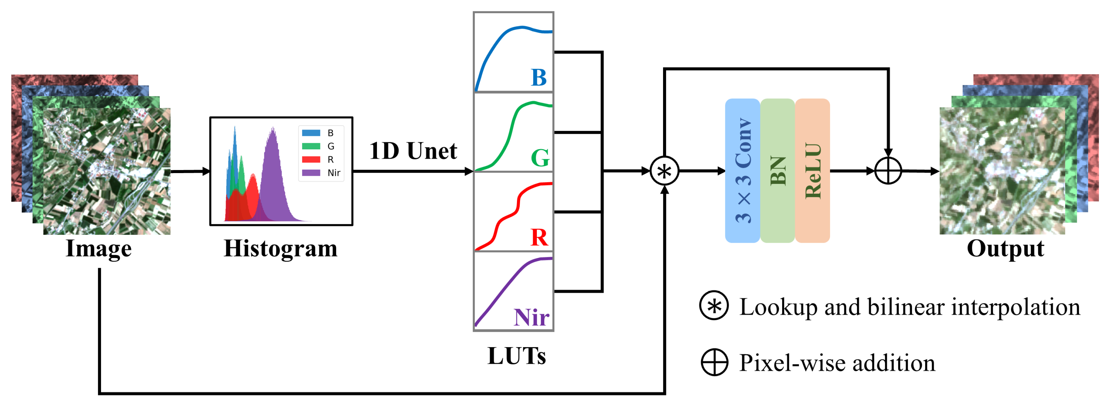
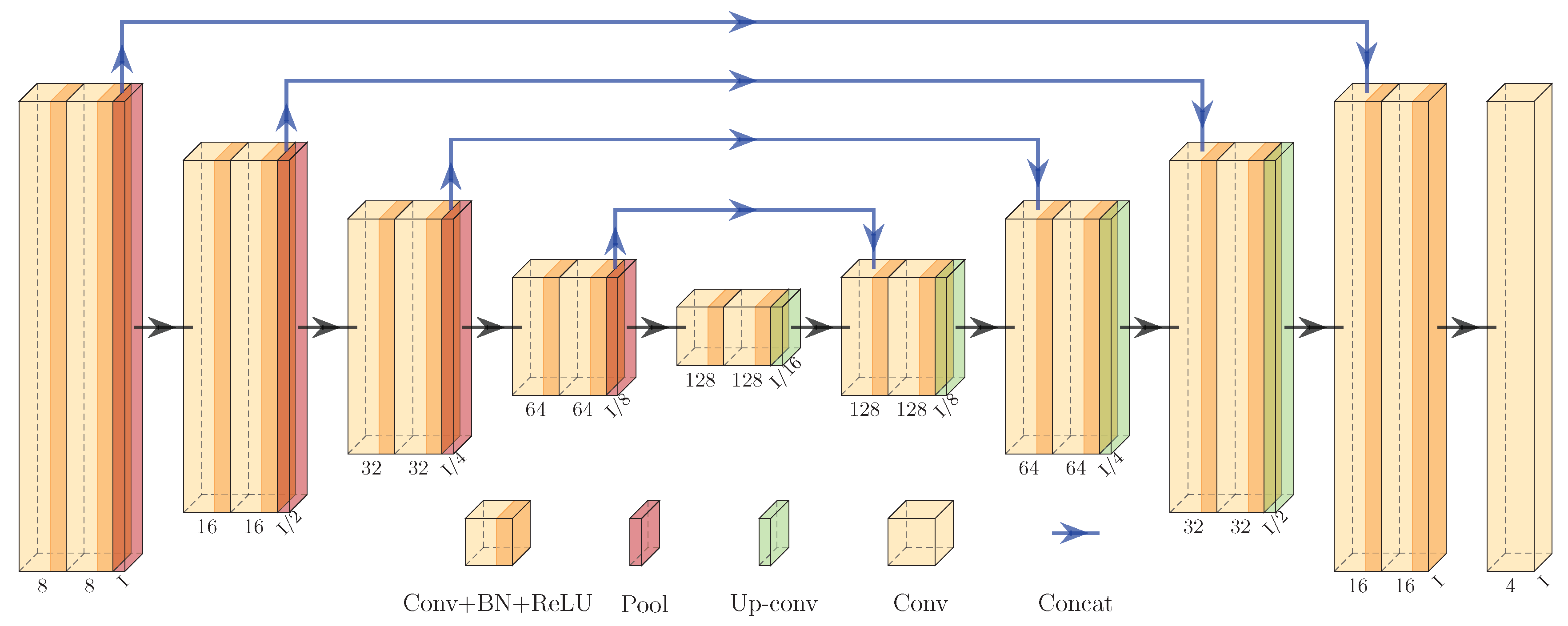
Guided by the above principles, we propose to learn tile-adaptive lookup tables (LUTs) with a U-shaped network (UNet) to produce fast and robust bandpass alignment. Inspired by the research of [30,33], the LUTs are used to enhance the linear model. The primary difference between our model and the preceding models is how the LUTs are learned. Our model generates the LUTs from the histogram of a tile, while these models are developed by images. As previously mentioned, the bandpass alignment can be regarded as an image enhancement task, and histogram matching is one of the most widely used methods. Histogram matching can be viewed as a process of finding LUTs based on the histograms of the input image pair. However, this is not applicable in our task since only the source S2 imagery is provided for the inference while the target GF1-ARD imagery is not. Motivated by the basic principles of histogram matching, we believe the expected LUTs are highly correlated with the input radiance distribution. Yet, it is challenging to learn a good mapping function from a histogram to LUTs. This issue can be effectively resolved by a deep learning model, which has strong non-linear and generalization abilities due to its deep structure. Therefore, we innovatively propose to learn tile-wise LUTs from the histograms of bands based on UNet. Furthermore, we add a single CNN layer with a $3\times 3$ kernel to lessen the burden of the registration error between S2 and GF1-ARD. Furthermore, such a small kernel hardly blurs the final output because the spatial resolution of the S2 input is inherently higher.

To validate the effectiveness of the proposed model, experiments have been conducted across two years at three diverse study sites. The radiance distribution and true colour images after the transformation are comprehensively visualized. Moreover, the normalized difference vegetation index (NDVI) is employed to demonstrate the excellent consistency of the temporally aligned data. The temporal frequency of data is further assessed to illustrate the giant promotion of the time series’ frequency after combining S2.

2. Materials and Methods

In this section, the basic configuration parameters of the GF1 data and processing of the L2A GF1-ARD products is introduced. Based on this, the procedure for dataset preparation for bandpass alignment is described. Finally, the architecture of the proposed model and training details are presented.

2.1. GF1-ARD Production

The GF1 satellite contains six CCD sensors, which take ground observations with three resolutions: 2 m (panchromatic band, PAN), 8 m (multispectral band, MS), and 16 m (WFV MS). The MS and WFV MS have the same spectral distribution, including visible and near-infrared bands as seen in Table 1. Specifically, two of the six sensors constitute an observation network producing PAN and MS imagery, while the other four CCDs produce WFV MS observations. In this paper, the archived level 1A GF1-WFV data with four multispectral bands (red, green, blue, and near-infrared) at 16 m spatial resolution and an 800 km swath width is selected to generate GF1-ARD. The level 1A GF1-WFV data only provide top-of-atmosphere (TOA) reflectance after systematic geometric processing. Howeverm problems prohibit the application of the GF1 data, including geometric offset, radiometric inconsistency, and atmospheric effects [37].

Figure 1 describes the procedure for processing the GF1-WFV L1A data into L2A products, designed to address the previously mentioned issues. Meanwhile, their distribution is shown in Figure 2. Firstly, radiometric calibration is carried out with the corresponding radiometric coefficients and then the atmospheric correction is implemented to remove atmospheric effects. The global mosaic Landsat-TM data (14.25 m) is then selected as the reference image to achieve the relative geometric precision correction due to the Landsat data’s sub-pixel geometric accuracy. Next, the quality assessment is conducted to label the land, water, cloud, cloud shadow, and snow pixels. In the end, the processed data is projected and tiled to the MGRS, consistent with S2.

2.2. Dataset

We developed a bandpass alignment dataset with three research regions located throughout the world, as depicted in Figure 2. These three regions are located in completely distinct environments, and the significant disparities in their spatial positions lead to variations in their landscape patterns and the corresponding reflectance characteristics. Consequently, we believe that the universality of our dataset and the generalization of the evaluated model can be guaranteed.

In order to minimize the impact of various factors brought by different observation conditions, the S2 L2A products are selected and the level 1A GF1-WFV data are processed to level 2A GF1-ARD since both have been corrected to SR. Furthermore, as shown in Figure 1, we have performed multiple rounds of filtering to assure the diversity and quality of our dataset. First, all the GF1–S2 pairs are observed on the same day. The same day acquisitions can assure that there is no change on the ground surface between the S2- and GF1-identified observations. Meanwhile, little variation is assumed in the Sun zenith, atmospheric conditions, or solar azimuth angles. As a result, any variations between the S2 and GF1 same-day collections are therefore exclusively regarded as differences in sensor responses [15]. These same-day pairs are then screened by cloud cover and overlapped area, and those with excessive cloud cover or insufficient overlapped area are excluded. Finally, a pair of GF1–S2 pairs is identified on a tile, with the guidance of distributing the data as evenly as possible across twelve months. Notably, for intersecting grids, we select data from as many different months as possible to increase data diversity and avoid subsequent data leakage issues. For example, on the 49TGE and 50TKK tiles, we select data from September to December, respectively.

After the same-day pairs are determined, the tile images are further processed to samples to be fed into the proposed network. The four multispectral bands with a spatial resolution of 10 m are firstly extracted. These bands are then resampled to 16 m with cubic convolution interpolation due to the mismatch between the spatial resolution of the S2 and GF1-ARD products. Following this, a mask is created to eliminate clouds, cloud shadows, and edge pixels with no data. The mask is created using the quality assessment bands and are eventually manually corrected. A tile imagery is then cropped into patches of $512\times 512$ pixels guided by the previously created mask, with patches with an effective pixel ratio of less than 0.8 being abandoned. Finally, these legal patches are randomly divided into training, validation, and test dataset with a ratio of nearly 1:1:2. The detailed sample distribution is detailed in

Table 2. Basic information of the dataset, including the location, date, and involved tile number of three study sites. Patch numbers are also provided for the training, validation, and test datasets.

Region	Location	Year	Tile	Training	Validation	Test
A	China	2020	69	1511	1360	2875
B	Brazil	2019	32	450	439	841
C	France	2020	92	2381	2273	4785
Sum	-	-	193	4341	4072	8501

. Meanwhile, the time distribution of training, validation, and test datasets are described in Figure 3.

2.3. Model Architecture

Figure 4 shows an overview of the proposed bandpass alignment framework. The entire network can be decomposed into two steps. First, we develop a UNet to generate band-wise LUTs to implement intensity transforms. Then, a small CNN is employed to supplement spatial details, performing local geometric correction. Subsequently, each component is described as follows.

2.3.1. LUTs

As previously mentioned, a rough pixel-wise transformation is anticipated because spatial details will be barely lost. Since the capability of the linear model is not satisfactory, a more powerful pixel-wise method is desired. A three-dimensional (3D) LUT is a traditional, efficient and popular technique for image enhancement [30]. It is exploited to adjust the hue, saturation, exposure, colour and tone of photos [38]. However, using a 3D LUT to remote sense multispectral imagery is impractical. For instance, the S2 MSI contains twelve bands and correspondingly requires a 12D LUT. The 3D grid defined by a 3D LUT consist of $M^3$ parameters, where M indicates the number of bins in each channel. Thus, it is a impossible to determine $M^{12}$ parameters of a 12D LUT. Meanwhile, it is unnecessary to consider the cross-channel interactions in SR imagery because there are no intersections between the band distributions. Therefore, multiple 1D LUTs are adopted, which solely consist of $12M$ elements. It is worth mentioning that 1D LUTs will degrade to a linear model when the values of LUTs are linearly corresponded with the input.

The bandpass alignment in LUTs is performed by two basic operations: lookup and bilinear interpolation. An input vector $I\left(p\right)=[I_n\left(p\right),n=1,\dots ,N]$ denotes the reflectance values of N bands located in a pixel p. Furthermore, Let $W\in {\mathbb{R}}^{N\times M}$ represent LUTs, whose element $w_{n,m}$ maps the reflectance m in the n-th band to reflectance $w_{n,m}$. A lookup manipulation is to find its location $(x_1,\dots ,x_N)$ in multiple LUTs:

$$x_n=\frac{I_n\left(p\right)}{s},n\in [1,N]$$

(1)

where $s=C_{max}^n/M$ with $C_{max}^n$ denoting the maximum reflectance value in the n-th band. After this, the interpolated values are calculated by bilinear interpolation. The transformed output intensity vector $I^{\prime }\left(p\right)$ is determined as follows:

$$I^{\prime }\left(p\right)=[(1-d{x}_n)\times w_{n,x}+d{x}_n\times w_{n,x+1},n=1,\dots ,N]$$

(2)

where $x=\lfloor x_n\rfloor ,d{x}_n=x_n-x$, and $\lfloor ·\rfloor$ is the floor operation. This bilinear interpolation is differentiable, and thus the pixel-wise operation can be optimized in parallel by GPU.

2.3.2. Learning LUTs

Ideally, globally shared LUTs are the best solution. However, due to various factors brought by diverse observation conditions, global LUTs are not applicable to numerous scenes. Since we have observed a high correlation between the input intensity distribution and the expected LUTs, we propose to generate LUTs from the histogram of a tile ($6863\times 6863$ pixels). In contrast, current models are developed by an image patch (such as $512\times 512$ pixels). On the one hand, the tile-wise LUTs are on a relatively larger scale compared to the image-adaptive LUTs. On the other hand, it is impractical to feed an entire imagery tile into a deep CNN because this will exceed the maximum memory of the machine, and it is completely unnecessary.

In particular, we model LUTs from histograms using a 1D UNet, an adaptation of the popular UNet [39]. The architecture of the 1D UNet is modified to the 1D signal processing scenario. As presented in Figure 5, it has a fully convolutional encoder–decoder type architecture. The encoder is composed of a repeated configuration of double $3\times 3$ convolutions with a stride of 1, each followed by a batch normalization (BN) [40] layer and a rectified linear unit (ReLU) [41], and a $2\times 2$ max pooling layer. At each contracting step in the encoder, the channels of the feature map are doubled while its size is halved. The upsampling step in the decoder step begins with a $2\times 2$ up-convolution, which halves the feature map channel. Furthermore, a concatenation operation with the corresponding feature map from the contracting path, and two $3\times 3$ convolutions with a stride of 1, each followed by a BN layer and an ReLU, are stacked. Finally, a $3\times 3$ convolutions with a stride of 1 is employed to output the transformed results.

Specifically, these LUTs are trained by the UNet together, and the input channels are therefore set to the band number N. It is worth noting that the tile number is limited. For example, there are only approx. one hundred tiles involved in France, far from enough for deep learning. In practice, we adopt different strategies in training and inference processes. The image-wise histograms are exploited in training, while tile-wise histograms are exploited in the inference process.

2.3.3. Supplementing Spatial Details

As mentioned previously, there exists a geometric registration error between the S2 L2A and GF1-ARD products even though S2 imagery is downsampled from 10 m to 16 m. Meanwhile, the reflectance transformation with the LUTs is pixel-by-pixel after the LUTs are acquired by the UNet. This pixel-level registration error is unacceptable for pixel-wise transformation. The issue can be alleviated by a convolutional operation with a receptive field greater than 1. However, the output of this convolution layer will be inevitably more fuzzy because the output value can be regarded as a kind of average value of pixels in the receptive field. For a good trade-off between spatial details and alignment, we thus add a $3\times 3$ convolutional layer with four kernels, followed by a BN layer and an ReLU. Specifically, the output of the LUT transformation is feed into the single layer CNN, and the results are the pixel-wise addition of them.

2.4. Criterion

Similar to [30], the proposed model is trained with mean-squared-error (MSE) loss and two regularization terms. Since the LUTs only learned with MSE loss are unsmooth, the abrupt value changes in neighbouring elements in the LUTs may lead to inconsistencies. The smooth regularization term $R_s$ and monotonicity regularization term $R_m$ are introduced to make the learned LUTs more stable and robust:

1.

MSE loss. Suppose there are K training samples ${\{x_i,y_i\}}_{k=1,2,\dots K}$, where $x_k$ denotes the k-th S2 patch and $y_k$ indicates the k-th GF1-ARD patch. The MSE loss is expressed as follows:

$$L_{MSE}=\frac{1}{K}\sum _{k=1}^K\left|\right|{\widehat{y}}_k-y_k{\left|\right|}^2$$

(3)

where the ${\widehat{y}}_k$ is the prediction of our model with $x_k$ as the input.

2.

Smooth regularization term. In order to stably transform the S2 bands into the GF1-like bands, the values in the LUTs should be locally smooth. In other words, it is expected that the learnt LUTs will vary slightly over a small range of input radiance. The smooth LUTs are define as follows:

$$R_s=\sum _{n=1}^N\sum _{x=1}^{M-1}\left|\right|(w_{n,x+1}-w_{n,x}){\left|\right|}^2$$

(4)

where n is the band index, N denotes the band number, x is calculated by Equation (1) and the floor operation, M is the number of bins in each band, and $w_{n,x}$ indicates the corresponding values in the LUTs. Meanwhile, the $L_2$ distance is employed for smoother regularization rather than the $L_1$ distance.

3.

Monotonicity regularization term. In addition to being smooth, LUTs should also be monotonic for two purposes. First, the relative reflectance value can be maintained, which is beneficial for ensuring the consistency before and after the transformation. Moreover, there might be insufficient training examples available in practice to cover the entire space of the LUTs, especially the two sides of the LUTs. Specifically, only a tiny portion of pixels in cloudless and snowless regions have reflectance values close to 1. Therefore, the generalization capability of the LUTs can be promoted when the monotonicity is ensured. The monotonicity regularization on the LUTs is formulated as follows:

$$R_m=\sum _{n=1}^N\sum _{x=1}^{M-1}max(0,w_{n,x+1}-w_{n,x})$$

(5)

Finally, the joint criterion L can be expressed as:

$$L=L_{MSE}+{\lambda }_s{R}_s+{\lambda }_m{R}_m$$

(6)

where ${\lambda }_s$ and ${\lambda }_m$ are the weight coefficients used to balance the effects of the smooth and monotonicity regularization terms, respectively.

We use the Adam optimizer [42] with a constant learning rate of $0.001$ to train the proposed model for 200 epochs, with four examples per mini-batch. The M, ${\lambda }_s$, and ${\lambda }_m$ are set to 256, $0.01$, and $0.01$, respectively. All hyperparameters are determined by the performance in the validation dataset with the early stopping strategy [43], and the same hyperparameter configuration is used for both the quantitative and qualitative results. Our code (code is available at https://github.com/Liuzhizhiooo/Bandpass-Alignment-UNet-LUT) is implemented with Python 3.8 and PyTorch 1.10.0 and will be accessible on 1 October 2023.

3. Results

In the following experiments, the proposed model is evaluated on our dataset. The linear model learned by ordinary least squares (OLS) is compared to illustrate the competitive performance of our model. The ablation study and visualization results are shown to demonstrate the effectiveness of this model. Moreover, the temporal frequency of the data is assessed after the bandpass alignment. Finally, the temporal consistency of the combined time sequence is measured.

3.1. Performance Comparison

The coefficient of determination ($R^2$) is adopted to quantify the goodness of fit of the model. In this regression task, the $R^2$ is a statistical measure of how well the transformed S2 bands approximate the GF1-ARD bands. An $R^2$ of 1 indicates that the regression predictions perfectly fit the data. In addition, we calculate the root-mean-squared error (RMSE) to measure the absolute difference between the prediction results and the ground truth. The smaller the difference between these the values pairs, the closer the relationship. Moreover, the OLS regression is derived between equivalent bands from the S2 and GF1-ARD, and the fitting model is formulated as follows:

$$y=slope\times x+intercept$$

(7)

where y is the GF1-ARD product and x is the prediction result, which can be the output of the linear model or our model.

Table 3. Quantitative comparison between the linear and proposed models in the blue, red, green, and NIR bands.

Model	Band	Slope	Intercept	${\mathit{R}}^2$	RMSE
Linear model	blue	0.487	0.097	0.473	0.022
	green	0.546	0.071	0.586	0.019
	red	0.640	0.048	0.795	0.022
	NIR	0.718	0.056	0.623	0.032
Ours	blue	1.117	−0.013	0.784	0.012
	green	1.026	−0.002	0.828	0.012
	red	1.061	−0.005	0.904	0.014
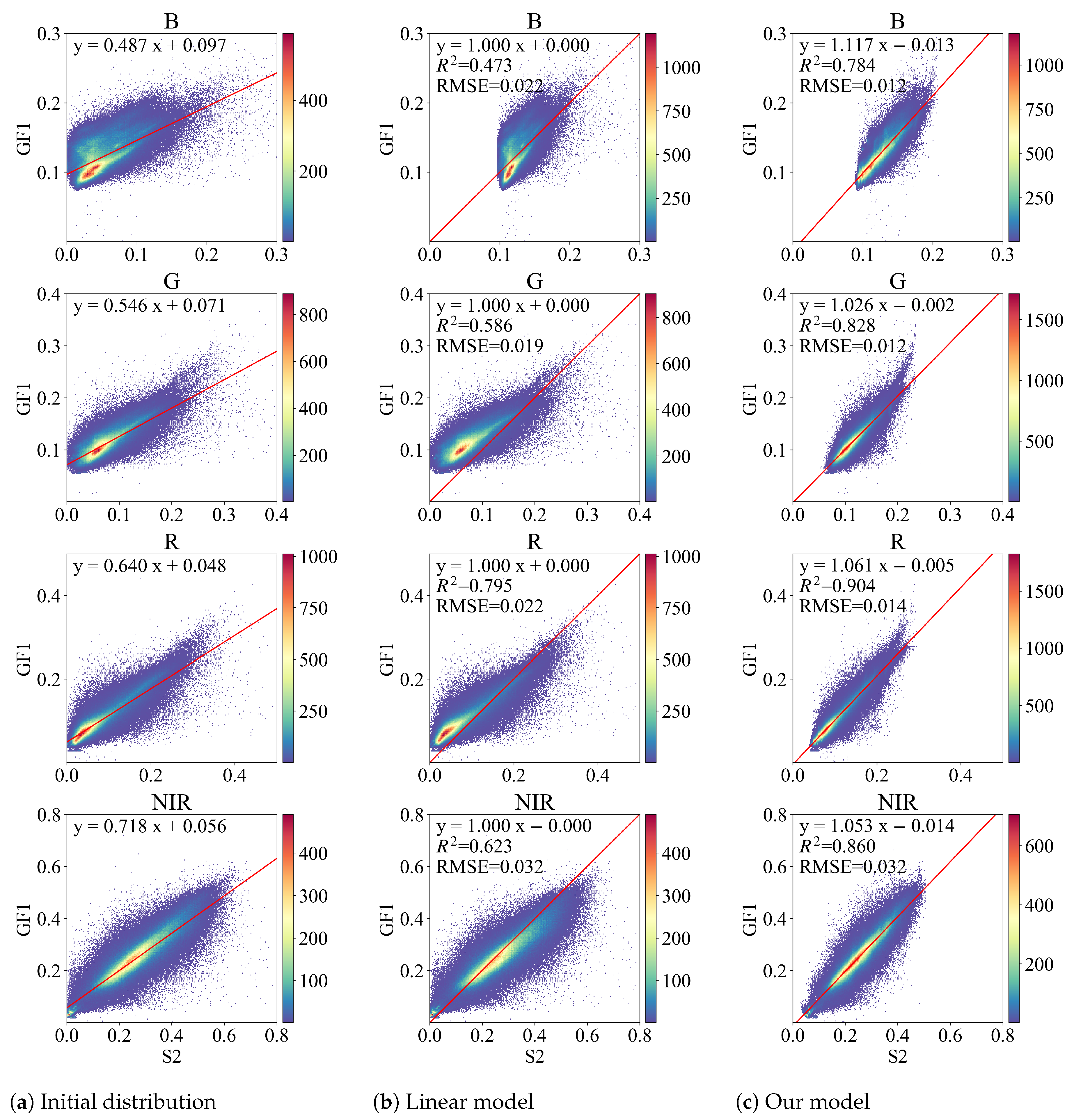
	NIR	1.053	−0.014	0.860	0.032

presents a quantitative comparison between the linear and proposed models in the test dataset. We observed that the linear correlation between S2 and GF1-ARD, especially in the blue band, is not significant enough. The $R^2$ values in blue, red, and NIR bands are less than 0.8, and those in the blue band are even less than 0.5. In contrast, the linear correlation between the GF1-ARD and the prediction of our model is greatly improved. The $R^2$ values of all bands are close to or greater than 0.8. In addition, the RMSE values are considerably lower than those of the linear model, especially the RMSE in the blue band, which is almost reduced by a factor of 2.

Figure 6 further displays the scatter plots between the GF1-ARD and different variables, including the initial S2 data and the prediction of the linear model and the output of our model. The parameters of the linear and proposed models are determined by samples in the training dataset. It is worth noting that the red solid line in Figure 6a is learned using OLS regression with the S2 and GF1-ARD representing the x and y in Equation (7), consistent with Table 3. Since the OLS is a linear transformation, the line fitted by the S2 after OLS transformation and GF1-ARD is $y=x$. Meanwhile, the red line in Figure 6c is learned with the prediction of our model and the GF1-ARD. As seen in Figure 6a, the scatters are not well located around the red solid line calculated by OLS regression, indicating a low linear correlation between S2 and GF1-ARD. In contrast, the scatters of our model are distributed more tightly, consistent with the previous quantitative results.

However, there still exists scatters that fall far apart and cannot be transformed well by our model. The remaining differences are caused by several factors, including misregistration, different viewing geometry, and mixed pixels. Despite the fact that our model employs a CNN module, the registration error cannot be fully addressed because a $3\times 3$ local operation cannot perfectly align the S2–GF1 pair spatially. Meanwhile, the viewing geometry differs even though the S2–GF1 pairs are observed on the same day. Correspondingly, the reflectance may vary greatly due to the terrain, particularly in mountain shadow regions. Moreover, the effects of mixed pixels vary because of the difference in spatial resolution. We downsampled S2 from 16 m to 30 m in the data processing, whereas the mixed pixels in the downsampled S2 are still less than those in the 30 m GF1-ARD. As a result, even if our model is powerful, the bandpass alignment will never be perfect because the observation conditions cannot be strictly identical.

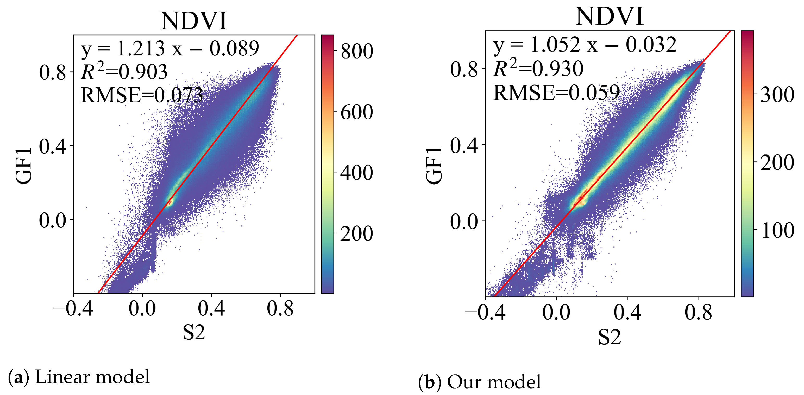
Furthermore, since the NDVI is one of the most simple yet effective vegetation indices, we extends the quantitative comparison to the NDVI. The NDVI is calculated using two bands by the following formula:

$$NDVI=\frac{{\rho }_{NIR}-{\rho }_R}{{\rho }_{NIR}+{\rho }_R}$$

(8)

where ${\rho }_{NIR}$ and ${\rho }_R$ stand for the reflectance in the near-infrared (NIR) and red bands, respectively. An NDVI value near one indicates a high level of green plant cover, while a value near zero denotes a lack of vegetation, possibly in urban areas. Water, clouds, or snow are the primary causes of negative NDVI values. The quantitative and qualitative results are shown in

Table 4. Quantitative comparison between the linear and proposed models in the NDVI.

Model	Band	Slope	Intercept	${\mathit{R}}^2$	RMSE
Linear model	NDVI	1.213	−0.089	0.903	0.073
Ours	NDVI	1.052	−0.032	0.930	0.059

and Figure 7, respectively. Even when $R^2$ for the red and NIR bands is less than 0.8, the linear model’s NDVI $R^2$ can reach 0.9, which can be attributed to two factors. First, the red and NIR bands have a relatively stronger linear correlation. Second, normalization enables the NDVI to be a successful descriptor of vegetation variations in the presence of atmospheric effects, sensor calibration degradation, and radiometric degradation in the red and NIR bands (reviewed by [44]). Our model increases the NDVI $R^2$ even higher to 0.93 while decreasing the RMSE from 0.073 to 0.059. Accordingly, the scattering points in Figure 7b are more centred around the red fitting line. Additionally, we find that the fitting is worse in areas with reflectance values lower than 0, which should be the area devoid of vegetation. As a result, the NDVI $R^2$ can be further promoted in practical applications, and we believe that the data that our model transforms is acceptable for qualitative and quantitative vegetation cover analysis.

3.2. Ablation Study

The improvement in the performance of our model can be attributed to two designs: the histogram-based LUTs and the CNN module. The following experiments are extended to illustrate the validity of these factors. It is worth noting that hyperparameters in the ablation experiments remain unchanged unless otherwise specified, and the early stopping strategy is adopted to select the best model. To better explore these two factors, we design several comparable models based on the proposed model. The “GlobalLUTs” refers to a global shared LUT model that has no relation to the tile histograms, whereas “TileLUTs” indicates a model that is based on the tile histograms. Moreover, a CNN module is added when the model name is suffixed with “-Conv”. All these comparisons are shown in

Table 5. Quantitative comparison of the ablation models.

Model	Histogram	CNN	Band	${\mathit{R}}^2$	RMSE
GlobalLUTs	✗	✗	blue	0.467	0.018
			green	0.701	0.015
			red	0.836	0.019
			NIR	0.788	0.040
GlobalLUTs-Conv	✗	✓	blue	0.563	0.017
			green	0.769	0.013
			red	0.893	0.015
			NIR	0.853	0.033
TileLUTs	✓	✗	blue	0.772	0.012
			green	0.785	0.013
			red	0.865	0.017
			NIR	0.811	0.038
TileLUTs-Conv (ours)	✓	✓	blue	0.784	0.012
			green	0.828	0.012
			red	0.904	0.014
			NIR	0.860	0.032

.

Table 5 presents the quantitative results of the comparable models, and we find that both factors are important. Since $R^2$ can better describe the differences in model performance, we focus more on it in the following analyses. Histogram-based LUTs are far more powerful than global LUTs, which boost the $R^2$ of GlobalLUTs and GlobalLUTs-Conv by nearly 0.3 and 0.2, respectively, in the blue band. The tile-adaptive transformation can adjust the LUTs in different scenes, allowing it to succeed in the blue band with low linear correlation. At the same time, we discover that the improvement in the other three bands is less obvious, because their linear correlations prior to transformation are higher than that of the blue band. In addition, the CNN module also plays an important role in our model. The CNN model benefits both the GlobalLUTs and TileLUTs, increasing the $R^2$ in the NIR band by nearly 0.07 and 0.05, respectively. Since the kernel size of the CNN module is only three, this finding demonstrates that even the pixel-level registration error matters in the bandpass alignment task. The positive effects of the CNN module are illustrated in Section 3.3.4.

3.3. Visualization Results

3.3.1. True Colour Combination

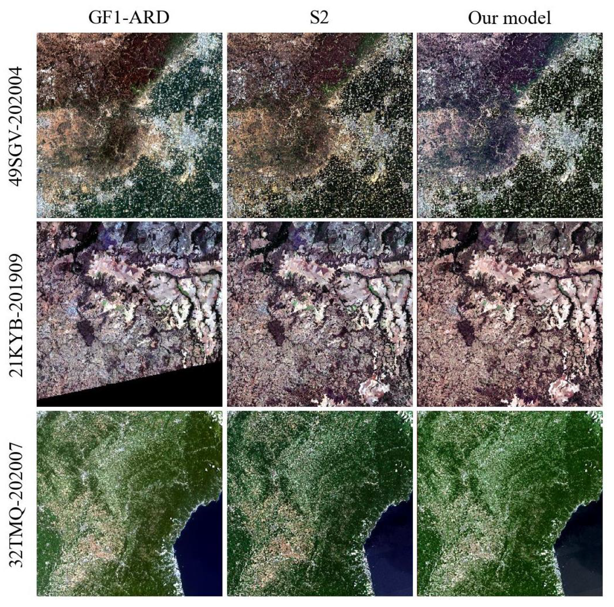
To better visualize the transformed imagery, we exhibit the true colour combination of tiles. Notably, the reflectance products are multiplied by 10,000 before being saved as UInt16 data. Hence, a mapping function is required to display the images. However, the dynamic stretching methods based on histogram statistics are not desirable in this case. Under different stretching parameters, the relative values of pixels cannot be maintained. As a result, this makes it impractical to evaluate the similarity between the transformed image and the target image. Therefore, the fixed-parameter stretching shown in

Table 6. The detail configuration of the fixed-parameter stretching.

Data Type	Band	Background	Linear Stretch	Saturate
UInt16	red	0–400	401–2000	>2000
	green	0–600	601–2000	>2000
	blue	0–800	801–2000	>2000
Byte		0	1–254	255

is adopted to present the imagery. The table records a three-stage stretching in which the values in the last three columns of UInt16 are mapped to the corresponding values of Byte.

Figure 8 displays the stretched results of three tiles, which are spread across three study sites over different months. As can be seen, there exists significant variations between S2 and GF1-ARD after the fixed stretching. This implies that their reflectances vary greatly, consistent with the scatter distribution in Figure 6a. The transformed S2 images are much closer to the GF1-ARD after bandpass alignment, demonstrating the necessity of it before combining multiple sensors. In addition, the overall colour of our model’s prediction is more realistic and closer to the target, whereas the linear model’s tends to whiter.

3.3.2. Batch Visualization

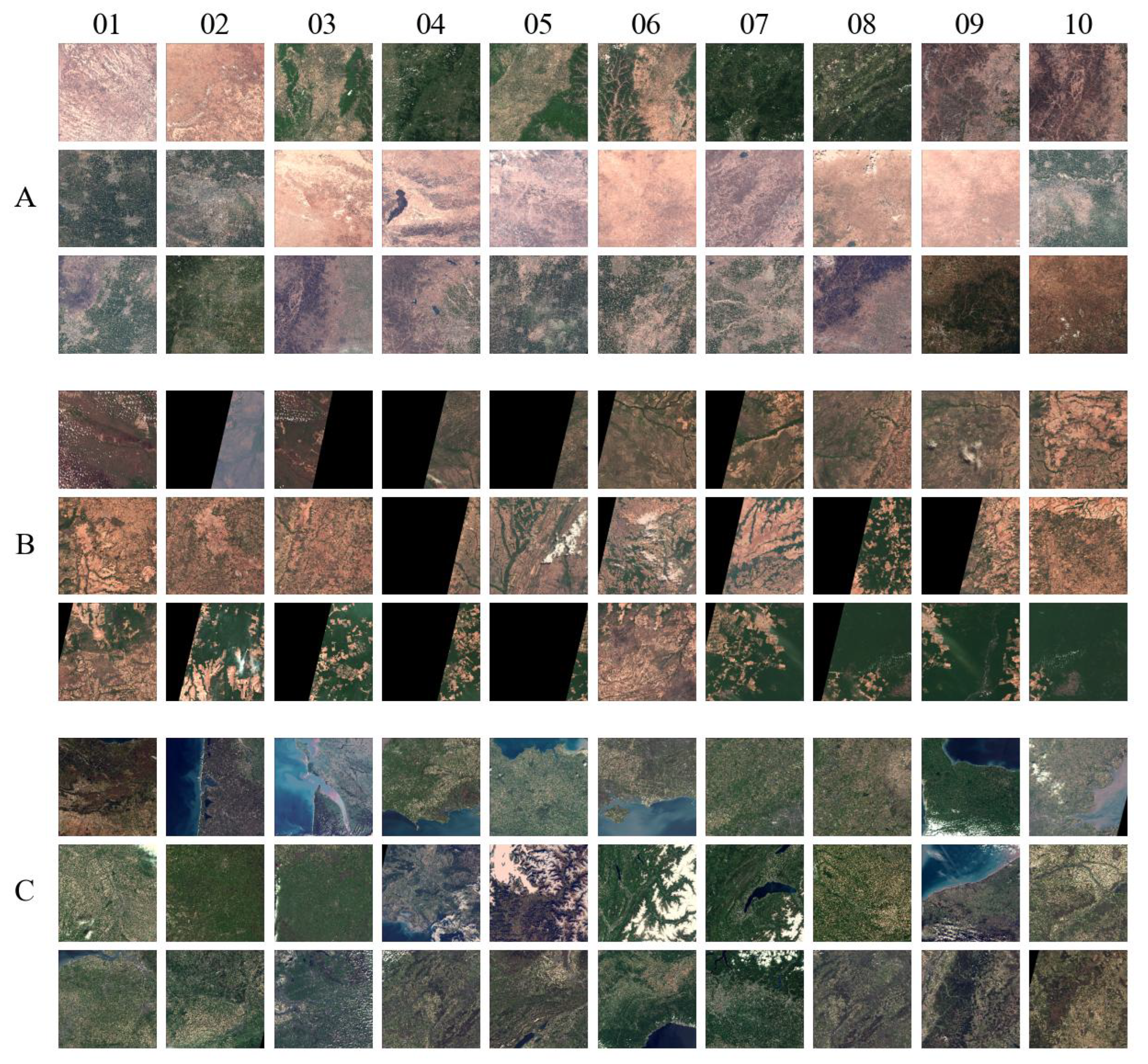
The ultimate goal of our model is to automatically batch transform the S2 imagery into GF1-ARD products. The key processes of the proposed model are a lookup operation and a single $3\times 3$ convolution, both of which require little time and computation. Meanwhile, the tile-adaptive LUTs are created using a UNet with only 0.17 M parameters. As a result, our model supports batch conversion of large amounts of data. To exemplify this, we use the trained model to transform all involved tiles in our dataset and then count the time it takes. In the inferring phase, the conversion and thumbnail creation of these 119 tiles take a total of 785 s, with one tile taking an average of 4.1 s. Our experiments are carried out on a NVIDIA RTX A6000. In addition, thirty tiles are selected from each of the three study sites, and their true colour images are depicted in Figure 9.

3.3.3. Visualization of LUTs

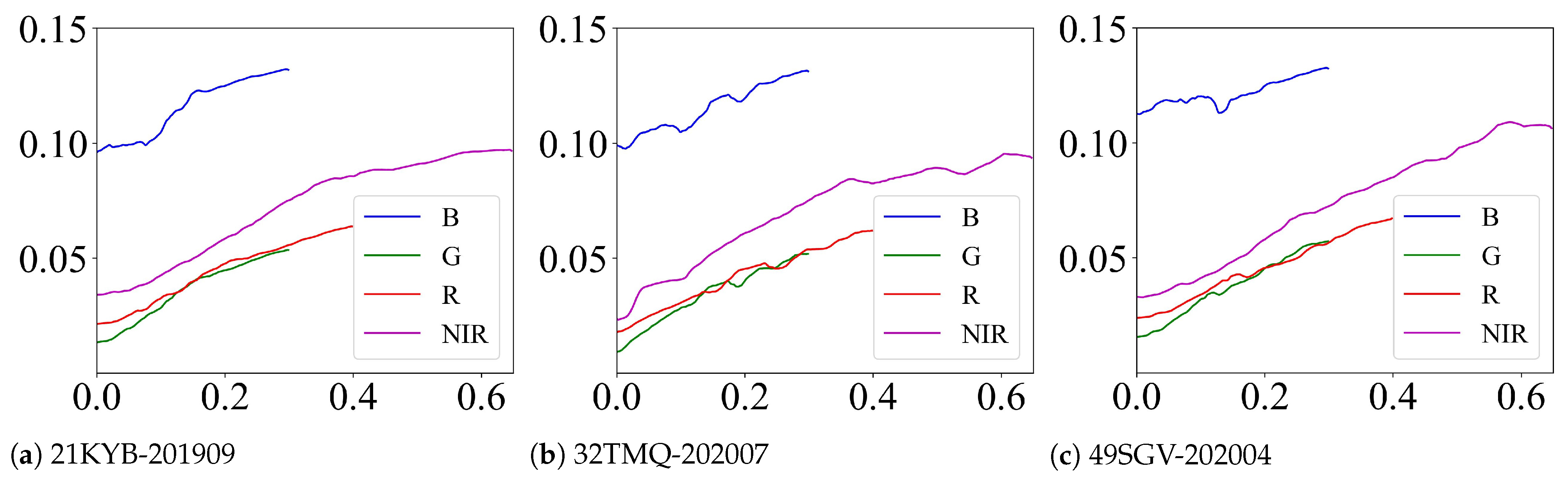
The LUTs of the previous three tiles are further displayed in Figure 10. The learned LUTs can describe a more complicated transformation function that the linear model cannot. For example, as the input increases, the LUTs of “21KYB-201909” tend to rise monotonically. The rising rate, however, varies in stages, with the rising rate at the beginning and end being gentler than in the middle. Meanwhile, we find that the LUTs of “49SGV-202004” approach linear transformation, consistent with the similar visualization results of the last row in Figure 8. Due to powerful capabilities of LUTs, the quantitative and qualitative results outperform the linear model. In addition, since most of the scatters are distributed in the former part of the space, we truncate the blue, green, red, and NIR bands with 0.3, 0.3, 0.4, and 0.6, respectively. Therefore, the length of the curve varies across the bands. As a result, the fixed-length LUT can be effectively exploited, and the degrees of fineness can be adaptively adjusted according to the distribution range of each band. Moreover, all the blue curves have a higher intercept value, which matches the scatter distribution of the blue band in Figure 6a.

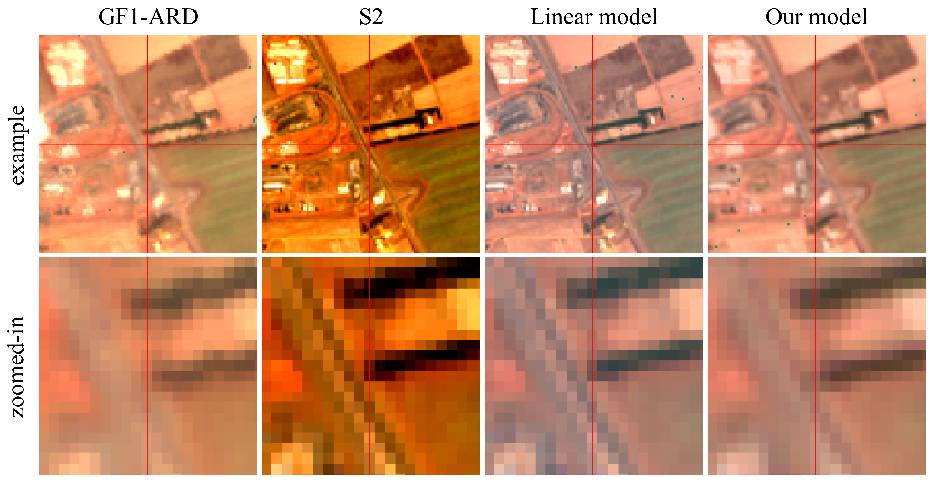
3.3.4. Spatial Misregistration

We select a local region in “21KYB-201909” as an example to present the spatial details of images in Figure 11. The first row shows the true colour combination of the selected local region. As previously mentioned, even though S2 is downsampled to 30 m, it still has more spatial details and sharper edges than GF1-ARD. The output of the linear model is as detailed as S2 because it is a pixel-wise transformation. In contrast, our model’s prediction is slightly blurrier than S2 since one $3\times 3$ convolutional operation is employed. However, the minor loss of spatial details makes it closer to the target GF1-ARD. In addition, we display zoomed-in views of the red cross point in the second row to illustrate the spatial misregistration between S2 and GF1-ARD. We find that there is one pixel offset in the row direction. Thus, the offset is preserved in the prediction of the linear model. In comparison, our model modifies the spatial location and approaches the target GF1-ARD, demonstrating the effectiveness of the simple CNN module. Meanwhile, we observe that there is still complex spatial distortion except for the pixel-level offset. This distortion is hard to eliminate and prevents further improvement of the bandpass alignment.

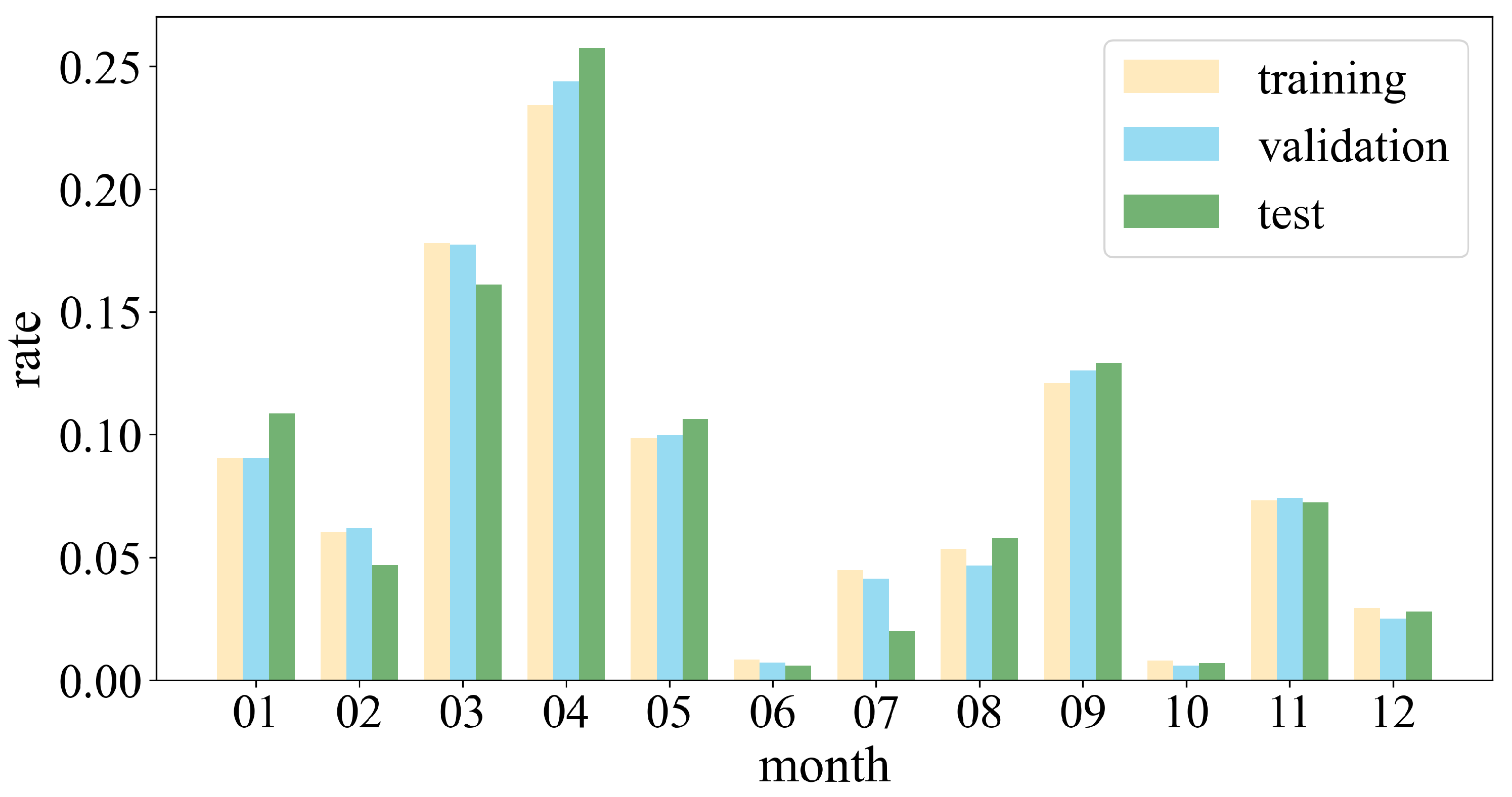
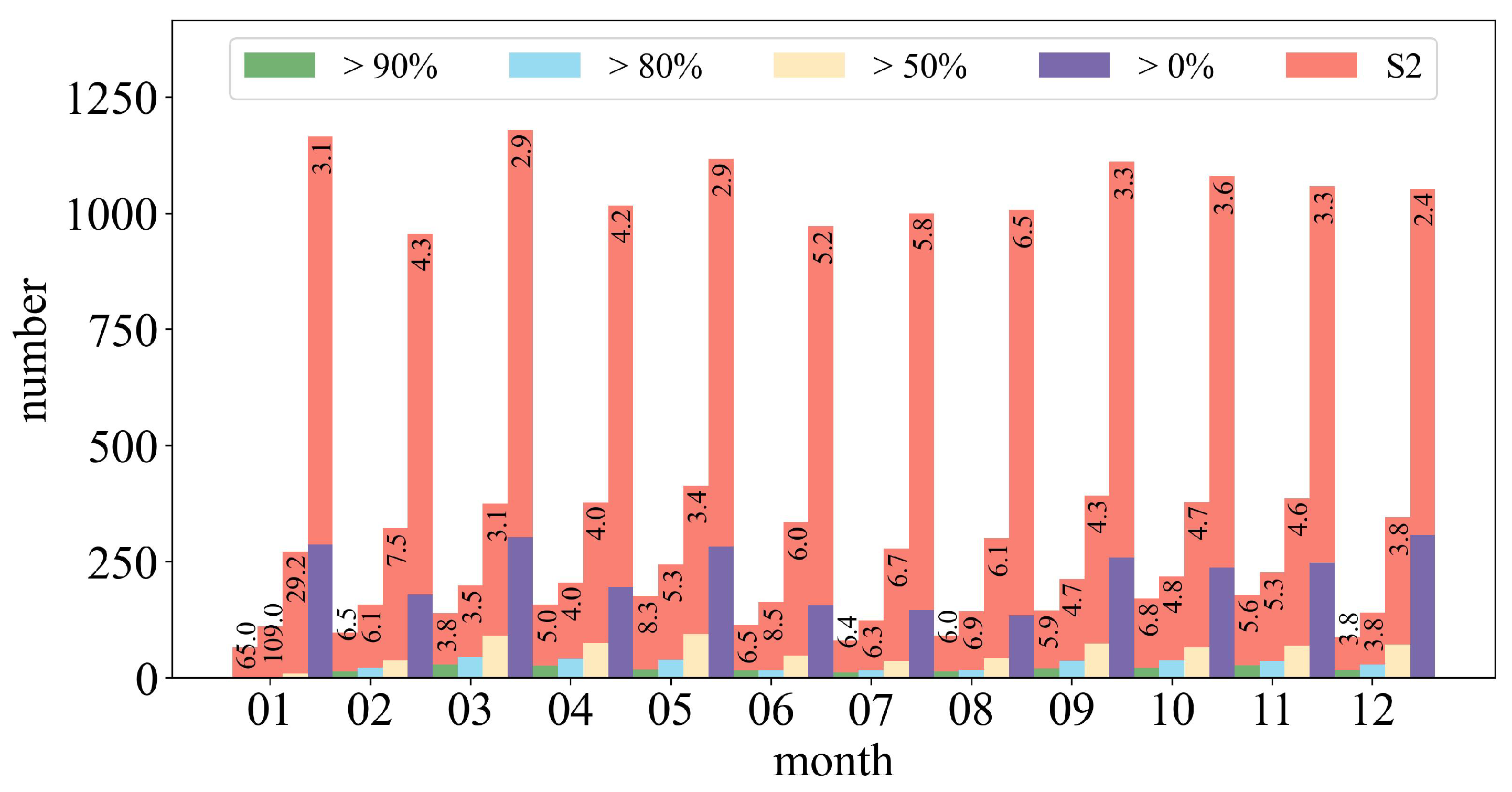
3.4. Temporal Frequency Assessment

We assess the volume of the S2 L2A and GF1-ARD images available at study site A (69 tiles in total) in 2020. Specifically, we investigate the amount at different valid data levels in Figure 12, where valid data refers to the pixels after removing no data and cloud regions.

We find that the total number of GF1-ARD data is large, while the expected data with a valid data rate greater than 80% are much lower. Meanwhile, the amount of valid data varies by month, and the volume decreases in summer and winter due to increased cloud cover, rain, and snow. For instance, in June, only seventeen images have a valid coverage ratio greater than 80%. Fortunately, the S2 to GF1-ARD ratio in these seasons is significantly higher than in others. After merging the S2 data, the temporal frequency of th eGF1-ARD data is significantly increased, which is critical in months when little data is available. Meanwhile, we find that the number of available data is drastically increased, even at the first levels, which greatly benefits the time series analysis.

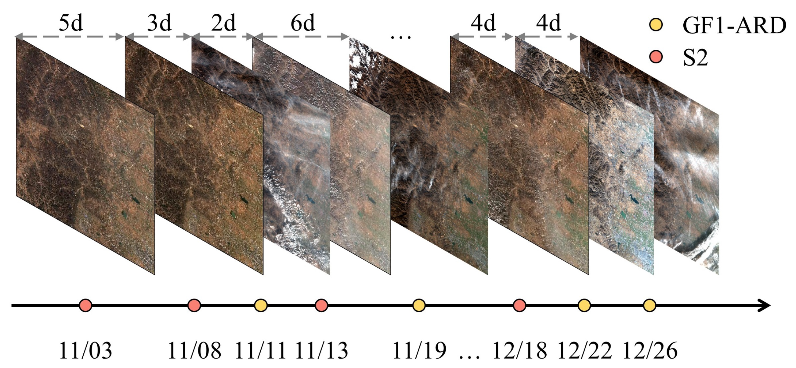
Furthermore, to better illustrate the combined effectiveness of merging the S2 data, we give an example of tile “49SGA” from November 2020 to December 2020 in Figure 13. To imitate the circumstances of practical application, the GF1-ARD with a valid data rate greater than 80% is filtered out, and there are only three images in two months. After combining the S2 data, the frequency of the collection is twice as dense as before. The distributions of the S2 and GF1-ARD are complementary, where the S2 has more data in November and the GF1 has more data in December. As a result, combining the data provides a much denser sequence with less cloud contamination.

4. Discussion

4.1. Variations between Adjacent Tiles

Since the key design of our model is the adaptive generation of LUTs, it is natural to explore the smoothness of the transition between adjacent tiles. The tile-adaptive LUTs are calculated using the input tile’s histogram. As a result, the learned LUTs vary across different tiles because their histograms are not identical, even when the tiles are adjacent and taken for the same day. As previously stated, the “GlobalLUTs” model avoids this problem by sharing the same LUTs on a global scale, but it is not flexible enough to fit various scenes or yield satisfactory results. Our model is therefore proposed to adaptively generalize distinct regions. Consequently, the differences between overlapping areas should be evaluated before transforming the S2 imagery in batches over large areas and producing seamless imagery. For each of the three study sites, we find four neighbouring tiles on the same day to visualize the variations in Figure 14. In addition, we carefully select four local regions located in the overlapping area and present their zoomed-in views.

Overall, the colour transition in the overlapped area is soft and smooth, and the mosaic results show almost no visible mosaic gap. The homogeneous mosaic results demonstrate our model’s reliable performance without any additional post-processing, such as feathering. Furthermore, at the bottom of Figure 14, we show zoomed-in views of various scenarios, including fields, rivers, the sea, buildings, and mountains. These views illustrate the high consistency of our results. The high similarity of histograms from adjacent tiles on the same day contributes to this result. Meanwhile, the slight difference in their histograms can be appropriately modelled by the powerful UNet. However, the high similarity between them cannot always be guaranteed, resulting in a relatively larger variation between the “50SKH” and “49SGB” tiles in the “A-20200412” mosaic. In the corresponding third zoomed-in view, the top half of the view tends to whiter. In addition, the one-pixel-width black edges caused by padding in the $3\times 3$ convolution operation can be resolved by replacing them with corresponding pixels in the neighbouring tiles.

4.2. Spatial Coverage of Histogram

Since the input histograms are patch-wise in the training phase, investigating the impact of the input histogram’s spatial coverage is required. We practically use patch- ($512\times 512$ pixels) and tile-wise ($6863\times 6863$ pixels) histograms in the training and inference phases due to limited tiles. Meanwhile, the patch size is also restricted to the maximum memory of the machine, which is a trade-off between performance and memory. Experiments are designed to investigate the influence of the exploited histograms in

Table 7. Quantitative comparison among histograms with different spatial coverages.

Patch Size	128		256		512 (Ours)
Band	${\mathit{R}}^2$	RMSE	${\mathit{R}}^2$	RMSE	${\mathit{R}}^2$	RMSE
Blue	0.763	0.012	0.766	0.012	0.784	0.012
Green	0.815	0.012	0.824	0.012	0.828	0.012
Red	0.893	0.015	0.898	0.015	0.904	0.014
NIR	0.847	0.034	0.857	0.033	0.860	0.032

. We have assessed the performance of the models trained with patches of different sizes. Except for the patch size, the model configuration, training strategy, and dataset division are all preserved in these experiments. As previously stated, the $R^2$ will be primarily compared.

We find that the performance increases as the patch size grows because larger patches can better simulate the histograms when inferring. However, we discover that the improvement over patch size is marginal, where the $R^2$ of the four bands increase by 0.018, 0.004, 0.006, and 0.003, respectively, when the patch size grow from 256 to 512. On the one hand, the input histograms have been normalized, which minimizes the adverse impact of dimensional disagreement. On the other hand, various histogram patterns are basically covered due to a larger amount of samples. As a result, the mismatch between the patch- and tile-wise histograms is reduced to a relatively minor level. Consequently, 512 is selected considering the machine memory and sample size.

Figure 14. Visualization of the variations between adjacent tiles. For each study site, four neighbouring tiles observed on the same day are selected to finish the image mosaic without any additional post-processing. Additionally, a mosaic is identified at the top and labelled using the “site-date” nomenclature. Meanwhile, the bottom of each mosaic presents four carefully chosen zoomed-in views in the overlapped regions, with the red boxes and corresponding number indicating where they are in the corresponding tile. All these images are shown with fixed-parameter stretching in Table 6.

Figure 14. Visualization of the variations between adjacent tiles. For each study site, four neighbouring tiles observed on the same day are selected to finish the image mosaic without any additional post-processing. Additionally, a mosaic is identified at the top and labelled using the “site-date” nomenclature. Meanwhile, the bottom of each mosaic presents four carefully chosen zoomed-in views in the overlapped regions, with the red boxes and corresponding number indicating where they are in the corresponding tile. All these images are shown with fixed-parameter stretching in Table 6.

4.3. Numerical Closeness versus Distributional Closeness

Although the learned model can maintain numerical similarity between predictions and targets, the distribution similarity is not explicitly guaranteed because the training criterion is MSE loss. The goal of our model is to make the transformed S2 imagery as close as possible to the target GF1-ARD, where the distance is defined as the Euclidean distance between pixels in all bands. Therefore, driven by the MSE loss, the optimizer tends to learn a transformation function that can ensure the numerical approximation. However, the histogram distributions of the predicted and target imagery are not guaranteed to be approximate. In order to demonstrate the histogram distribution variation, we select a widely used histogram-based stretching method: 2% clip stretching. The visualization results are shown in Figure 15. In addition, the linear model’s outputs are similar to the S2 because the global linear transform does not change the distribution, and thus are not shown.

The colour distortion between the predicted S2 and target GF1-ARD is more notable than between the input S2 and target GF1-ARD, especially in the “49SGV-202004”. Because the numerical differences between the images can be reduced after adaptive adjustments, S2 imagery approaches GF1-ARD more closely even with larger numerical differences. This discovery confirms the previous analysis that the MSE loss does not ensure distribution approximation. However, optimizing the model to achieve both numerical and distributional approximation is a difficult task. This issue will be further researched in the future.

5. Conclusions

In this paper, we proposed a UNet-based model to perform bandpass alignment, transforming S2 to GF1-ARD with tile-adaptive LUTs to generate higher-temporal-frequency continuous collections. In contrast to the linear model employed in prior work, LUTs are introduced to better describe the alignment function between sensors. With the assistance of tile histograms and a CNN module, the proposed model achieves approximately 0.31, 0.24, 0.11, and 0.23 improvements over the linear model in four spectral bands, respectively. In addition, we comprehensively conduct ablation experiments and numerous visualizations to evaluate the effectiveness of our model. We further discuss the key settings and analyse the underlying causes of the corresponding phenomena. In future work, we will consider employing other medium-resolution sensor data to further improve the temporal resolution of GF1-ARD, such as Landsat-8 OLI.

References

1. Claverie, M.; Ju, J.; Masek, J.G.; Dungan, J.L.; Vermote, E.F.; Roger, J.C.; Skakun, S.V.; Justice, C. The Harmonized Landsat and Sentinel-2 surface reflectance data set. Remote Sens. Environ. 2018, 219, 145–161. [Google Scholar] [CrossRef]
2. Sigurdsson, J.; Armannsson, S.E.; Ulfarsson, M.O.; Sveinsson, J.R. Fusing Sentinel-2 and Landsat 8 Satellite Images Using a Model-Based Method. Remote Sens. 2022, 14, 3224. [Google Scholar] [CrossRef]
3. Runge, A.; Grosse, G. Mosaicking Landsat and Sentinel-2 Data to Enhance LandTrendr Time Series Analysis in Northern High Latitude Permafrost Regions. Remote Sens. 2020, 12, 2471. [Google Scholar] [CrossRef]
4. Li, J.; Roy, D.P. A Global Analysis of Sentinel-2A, Sentinel-2B and Landsat-8 Data Revisit Intervals and Implications for Terrestrial Monitoring. Remote Sens. 2017, 9, 902. [Google Scholar] [CrossRef]
5. Zhu, Z.; Woodcock, C.E. Continuous change detection and classification of land cover using all available Landsat data. Remote Sens. Environ. 2014, 144, 152–171. [Google Scholar] [CrossRef]
6. Zeng, Y.; Hao, D.; Huete, A.; Dechant, B.; Berry, J.; Chen, J.M.; Joiner, J.; Frankenberg, C.; Bond-Lamberty, B.; Ryu, Y.; et al. Optical vegetation indices for monitoring terrestrial ecosystems globally. Nat. Rev. Earth Environ. 2022, 3, 477–493. [Google Scholar] [CrossRef]
7. Li, X.; Zhou, Y.; Zhu, Z.; Liang, L.; Yu, B.; Cao, W. Mapping annual urban dynamics (1985–2015) using time series of Landsat data. Remote Sens. Environ. 2018, 216, 674–683. [Google Scholar] [CrossRef]
8. Kuenzer, C.; Guo, H.; Huth, J.; Leinenkugel, P.; Li, X.; Dech, S. Flood Mapping and Flood Dynamics of the Mekong Delta: ENVISAT-ASAR-WSM Based Time Series Analyses. Remote Sens. 2013, 5, 687–715. [Google Scholar] [CrossRef]
9. Skakun, S.; Kussul, N.; Shelestov, A.; Kussul, O. Flood Hazard and Flood Risk Assessment Using a Time Series of Satellite Images: A Case Study in Namibia. Risk Anal. 2014, 34, 1521–1537. [Google Scholar] [CrossRef]
10. Dwyer, J.L.; Roy, D.P.; Sauer, B.; Jenkerson, C.B.; Zhang, H.K.; Lymburner, L. Analysis Ready Data: Enabling Analysis of the Landsat Archive. Remote Sens. 2018, 10, 1363. [Google Scholar] [CrossRef]
11. Ju, J.; Roy, D.P. The availability of cloud-free Landsat ETM+ data over the conterminous United States and globally. Remote Sens. Environ. 2008, 112, 1196–1211. [Google Scholar] [CrossRef]
12. Fu, P.; Weng, Q. Consistent land surface temperature data generation from irregularly spaced Landsat imagery. Remote Sens. Environ. 2016, 184, 175–187. [Google Scholar] [CrossRef]
13. Roy, D.; Kovalskyy, V.; Zhang, H.; Vermote, E.; Yan, L.; Kumar, S.; Egorov, A. Characterization of Landsat-7 to Landsat-8 reflective wavelength and normalized difference vegetation index continuity. Remote Sens. Environ. 2016, 185, 57–70, Landsat 8 Science Results. [Google Scholar] [CrossRef] [PubMed]
14. Flood, N. Comparing Sentinel-2A and Landsat 7 and 8 Using Surface Reflectance over Australia. Remote Sens. 2017, 9, 659. [Google Scholar] [CrossRef]
15. Runge, A.; Grosse, G. Comparing Spectral Characteristics of Landsat-8 and Sentinel-2 Same-Day Data for Arctic-Boreal Regions. Remote Sens. 2019, 11, 1730. [Google Scholar] [CrossRef]
16. Aydal, D.; Arda1, E.; Dumanlilar, Ö. Application of the Crosta technique for alteration mapping of granitoidic rocks using ETM+ data: Case study from eastern Tauride belt (SE Turkey). Int. J. Remote Sens. 2007, 28, 3895–3913. [Google Scholar] [CrossRef]
17. Vural, A.; Akpinar, İ.; Sipahi, F. Mineralogical and Chemical Characteristics of Clay Areas, Gümüşhane Region (NE Turkey), and Their Detection Using the Crósta Technique with Landsat 7 and 8 Images. Nat. Resour. Res. 2021, 30, 3955–3985. [Google Scholar] [CrossRef]
18. Wang, Q.; Blackburn, G.A.; Onojeghuo, A.O.; Dash, J.; Zhou, L.; Zhang, Y.; Atkinson, P.M. Fusion of Landsat 8 OLI and Sentinel-2 MSI Data. IEEE Trans. Geosci. Remote Sens. 2017, 55, 3885–3899. [Google Scholar] [CrossRef]
19. Shao, Z.; Cai, J.; Fu, P.; Hu, L.; Liu, T. Deep learning-based fusion of Landsat-8 and Sentinel-2 images for a harmonized surface reflectance product. Remote Sens. Environ. 2019, 235, 111425. [Google Scholar] [CrossRef]
20. Shi, W.; Guo, D.; Zhang, H. A reliable and adaptive spatiotemporal data fusion method for blending multi-spatiotemporal-resolution satellite images. Remote Sens. Environ. 2022, 268, 112770. [Google Scholar] [CrossRef]
21. Qiu, S.; Lin, Y.; Shang, R.; Zhang, J.; Ma, L.; Zhu, Z. Making Landsat Time Series Consistent: Evaluating and Improving Landsat Analysis Ready Data. Remote Sens. 2019, 11, 51. [Google Scholar] [CrossRef]
22. Roy, D.P.; Ju, J.; Lewis, P.; Schaaf, C.; Gao, F.; Hansen, M.; Lindquist, E. Multi-temporal MODIS–Landsat data fusion for relative radiometric normalization, gap filling, and prediction of Landsat data. Remote Sens. Environ. 2008, 112, 3112–3130. [Google Scholar] [CrossRef]
23. Nagol, J.R.; Sexton, J.O.; Kim, D.H.; Anand, A.; Morton, D.; Vermote, E.; Townshend, J.R. Bidirectional effects in Landsat reflectance estimates: Is there a problem to solve? ISPRS J. Photogramm. Remote Sens. 2015, 103, 129–135, Global Land Cover Mapping and Monitoring. [Google Scholar] [CrossRef]
24. Ju, J.; Roy, D.P.; Shuai, Y.; Schaaf, C. Development of an approach for generation of temporally complete daily nadir MODIS reflectance time series. Remote Sens. Environ. 2010, 114, 1–20. [Google Scholar] [CrossRef]
25. Markham, B.L.; Helder, D.L. Forty-year calibrated record of earth-reflected radiance from Landsat: A review. Remote Sens. Environ. 2012, 122, 30–40, Landsat Legacy Special Issue. [Google Scholar] [CrossRef]
26. Steven, M.D.; Malthus, T.J.; Baret, F.; Xu, H.; Chopping, M.J. Intercalibration of vegetation indices from different sensor systems. Remote Sens. Environ. 2003, 88, 412–422. [Google Scholar] [CrossRef]
27. Liu, K.; Su, H.; Li, X.; Wang, W.; Yang, L.; Liang, H. Quantifying Spatial–Temporal Pattern of Urban Heat Island in Beijing: An Improved Assessment Using Land Surface Temperature (LST) Time Series Observations from LANDSAT, MODIS, and Chinese New Satellite GaoFen-1. IEEE J. Sel. Top. Appl. Earth Obs. Remote Sens. 2016, 9, 2028–2042. [Google Scholar] [CrossRef]
28. Ghimire, P.; Lei, D.; Juan, N. Effect of Image Fusion on Vegetation Index Quality—A Comparative Study from Gaofen-1, Gaofen-2, Gaofen-4, Landsat-8 OLI and MODIS Imagery. Remote Sens. 2020, 12, 1550. [Google Scholar] [CrossRef]
29. LeCun, Y.; Bengio, Y.; Hinton, G. Deep learning. Nature 2015, 521, 436–444. [Google Scholar] [CrossRef]
30. Zeng, H.; Cai, J.; Li, L.; Cao, Z.; Zhang, L. Learning Image-Adaptive 3D Lookup Tables for High Performance Photo Enhancement in Real-Time. IEEE Trans. Pattern Anal. Mach. Intell. 2022, 44, 2058–2073. [Google Scholar] [CrossRef]
31. Gharbi, M.; Chen, J.; Barron, J.T.; Hasinoff, S.W.; Durand, F. Deep Bilateral Learning for Real-Time Image Enhancement. ACM Trans. Graph. 2017, 36, 118. [Google Scholar] [CrossRef]
32. Yan, Z.; Zhang, H.; Wang, B.; Paris, S.; Yu, Y. Automatic Photo Adjustment Using Deep Neural Networks. ACM Trans. Graph. 2016, 35, 11. [Google Scholar] [CrossRef]
33. Kim, H.U.; Koh, Y.J.; Kim, C.S. Global and Local Enhancement Networks for Paired and Unpaired Image Enhancement. In Proceedings of the Computer Vision—ECCV 2020, Glasgow, UK, 23–28 August 2020; Vedaldi, A., Bischof, H., Brox, T., Frahm, J.M., Eds.; Springer: Cham, Switzerland, 2020; pp. 339–354. [Google Scholar]
34. Ignatov, A.; Kobyshev, N.; Timofte, R.; Vanhoey, K. DSLR-Quality Photos on Mobile Devices with Deep Convolutional Networks. In Proceedings of the 2017 IEEE International Conference on Computer Vision (ICCV), Venice, Italy, 22–29 October 2017; pp. 3297–3305. [Google Scholar] [CrossRef]
35. Li, Y.; Gupta, A. Beyond Grids: Learning Graph Representations for Visual Recognition. In Proceedings of the NIPS’18, 32nd International Conference on Neural Information Processing Systems, Montreal, QC, Canada, 2–8 December 2018; pp. 9245–9255. [Google Scholar]
36. Liu, Z.Q.; Tang, P.; Zhang, W.; Zhang, Z. CNN-Enhanced Heterogeneous Graph Convolutional Network: Inferring Land Use from Land Cover with a Case Study of Park Segmentation. Remote Sens. 2022, 14, 5027. [Google Scholar] [CrossRef]
37. Zhong, B.; Yang, A.; Liu, Q.; Wu, S.; Shan, X.; Mu, X.; Hu, L.; Wu, J. Analysis Ready Data of the Chinese GaoFen Satellite Data. Remote Sens. 2021, 13, 1709. [Google Scholar] [CrossRef]
38. Karaimer, H.C.; Brown, M.S. A Software Platform for Manipulating the Camera Imaging Pipeline. In Proceedings of the Computer Vision—ECCV 2016, Amsterdam, The Netherlands, 11–14 October 2016; Leibe, B., Matas, J., Sebe, N., Welling, M., Eds.; Springer: Cham, Switzerland, 2016; pp. 429–444. [Google Scholar]
39. Ronneberger, O.; Fischer, P.; Brox, T. U-Net: Convolutional Networks for Biomedical Image Segmentation. In Proceedings of the Medical Image Computing and Computer-Assisted Intervention—MICCAI 2015, Munich, Germany, 5–9 October 2015; Navab, N., Hornegger, J., Wells, W.M., Frangi, A.F., Eds.; Springer: Cham, Switzerland, 2015; pp. 234–241. [Google Scholar]
40. Ioffe, S.; Szegedy, C. Batch Normalization: Accelerating Deep Network Training by Reducing Internal Covariate Shift. arXiv 2015, arXiv:1502. 03167. [Google Scholar] [CrossRef]
41. Nair, V.; Hinton, G.E. Rectified Linear Units Improve Restricted Boltzmann Machines. In Proceedings of the ICML’10, 27th International Conference on International Conference on Machine Learning, Haifa, Israel, 21–24 June 2010; pp. 807–814. [Google Scholar]
42. Kingma, D.P.; Ba, J. Adam: A Method for Stochastic Optimization. arXiv 2014, arXiv:1412.6980. [Google Scholar]
43. Prechelt, L. Early Stopping—However, When? In Neural Networks: Tricks of the Trade: Second Edition; Springer: Berlin/Heidelberg, Germany, 2012; pp. 53–67. [Google Scholar] [CrossRef]
44. Bannari, A.; Morin, D.; Bonn, F.; Huete, A.R. A review of vegetation indices. Remote Sens. Rev. 1995, 13, 95–120. [Google Scholar] [CrossRef]
Figure 1. The whole processing procedure of our dataset, including three components: GF1-ARD producing, data filtering, and data processing.
Remotesensing 15 02563 g001
Figure 2. The spatial distribution and division of our dataset over the MODIS-derived global green vegetation map. There are three study sites A, B, and C in our dataset, located in China, Brazil, and France, respectively. All these tiles are randomly divided into training–validation and test sets. The detailed division result is shown in the corresponding zoomed-in views. The yellow dot grid represents a tile containing both training and validation samples, while the green dot grid indicates a tile consisting of pure test samples. The samples in the yellow dot are then split into training and validation samples at a nearly 1:1 ratio.
Remotesensing 15 02563 g002
Figure 3. Distribution of the training, validation, and test datasets over twelve months.
Remotesensing 15 02563 g003
Figure 4. The architecture of the proposed model. It is composed of two components: 1D LUTs generation based on the U-shaped network (UNet) and a simple CNN module.
Remotesensing 15 02563 g004
Figure 5. The architecture of the 1D UNet. It is an encoder–decoder network with four layers in both the encoder and decoder. The initial input feature number is four, and the feature channel is doubled while the feature size is halved after passing one layer of the encoder. In contrast, after passing one layer of the decoder, the feature channel is halved while the feature size is doubled. Meanwhile, a concatenation operation is employed to merge features from different scales. Finally, a convolutional layer is applied to produce the outputs with the same channel number as the inputs.
Remotesensing 15 02563 g005
Figure 6. (a) Comparison of the surface reflectance (SR) from Sentinel-2 and GF1-ARD. (b) Comparison of the predicted SR by OLS and the GF1-ARD. (c) Comparison of the predicted SR by our model and the GF1-ARD. All of the above sub-graphs are drawn using data from the test set. The colour bar on the right is used to render the scatters, and the more red the points, the denser they are. The red solid line represents the line fitted by ordinary least squares (OLS). The accuracy indices root-mean-squared error (RMSE) and the coefficient of determination ( R 2 ) of the linear model are shown in the upper left corner.
Remotesensing 15 02563 g006
Figure 7. (a) Comparison of the normalized difference vegetation index (NDVI) from the adjusted Sentinel-2 by the linear model and GF1-ARD. (b) Comparison of the NDVI from the transformed Sentinel-2 by our model and GF1-ARD.
Remotesensing 15 02563 g007
Figure 8. Visualization results of the different methods. Three tiles of test dataset distributed at different study sites over several months are provided for comparison, identified at the left and labelled using the “tile-date” nomenclature. The first column is the GF1-ARD images, the second indicates the Sentinel-2 imagery, the third lists the prediction of the linear model, and the last column exhibits the transformed images of our model. All these images are shown with the fixed-parameter stretching in Table 6.
Remotesensing 15 02563 g008
Figure 9. Tile thumbnails of our model’s prediction. Thirty tiles are selected from three study sites, including China (A), Brazil (B), and France (C), and the outputs of our model are shown as thumbnails in three rows. All these images are shown with the fixed-parameter stretching in Table 6.
Remotesensing 15 02563 g009
Figure 10. The calculated LUTs of the three tiles. The first three bands are represented by corresponding colours, and the near-infrared band is rendered by a purple line. In addition, these bands are truncated by different values given the scatters.
Remotesensing 15 02563 g010
Figure 11. The comparison of spatial details. The first row shows the true colour combination of the selected local region in “21KYB-201909”. The second row displays the zoomed-in views of the red cross point in the first row, where all crosses share the same geometric position.
Remotesensing 15 02563 g011
Figure 12. The amount of S2 L2A and GF1-ARD imagery available at study site A in 2020. The detailed number of images under various valid data levels and months are displayed. The green, blue, and yellow bars represent the data with a valid data rate greater than 90, 80 50, and 0%, respectively. Meanwhile, the extended red bar refers to the corresponding S2 data, and the number at the top represents the ratio of S2 to GF1-ARD.
Remotesensing 15 02563 g012
Figure 13. An illustration of combining S2 and GF1-ARD. The yellow dot represents the GF1-ARD, and the orange dot refers to the S2 data. Meanwhile, the images are organized according to the time line below, with the days between images labelled above.
Remotesensing 15 02563 g013
Figure 15. Visualization results of the tiles in Figure 8 with 2% clip stretching.
Remotesensing 15 02563 g015