Article

Evaluating the Consistency of Vegetation Phenological Parameters in the Northern Hemisphere from 1982 to 2015

1
State Key Laboratory of Desert and Oasis Ecology, Xinjiang Institute of Ecology and Geography, Chinese Academy of Sciences, Urumqi 830011, China
2
University of Chinese Academy of Sciences, Beijing 100049, China
*
Author to whom correspondence should be addressed.
Remote Sens. 2023, 15(10), 2559; https://doi.org/10.3390/rs15102559
Submission received: 15 March 2023 / Revised: 3 May 2023 / Accepted: 9 May 2023 / Published: 13 May 2023

Abstract

:
Vegetation phenology reflects the response mechanisms in ecology and climate change, so it is important that the parameters used to study vegetation phenology are accurate. Previous studies mainly focused on phenological changes. However, because the extraction methods used in those investigations led to inconsistencies in setting vegetation phenological parameters, a more accurate approach needs to be developed. To resolve this issue, we select five methods to extract the start of the growing season (SOS) and the end of the growing season (EOS) from the normalised difference vegetation index (NDVI3g) data. The five chosen methods are the second-order derivative method (Method 1), the first-order derivative method (Method 2), the 0.2 dynamic threshold method (Method 3), the 0.5 dynamic threshold method (Method 4), and the fixed threshold method (Method 5). Our study area is the Northern Hemisphere (above 30°N), and our study period is 1982 to 2015. After applying the five methods, we evaluate the consistency of the vegetation phenological parameters. The results show that (1) regardless of the method used, the average changes in phenological parameters are consistent; however, the SOS and EOS under Methods 1, 3 and 5 are up to 30 days earlier than those under Methods 2 and 4. (2) Under all five methods, the SOS trend mainly shows an advance, but the trend is substantially higher under Methods 1, 3 and 4 than under Methods 2 and 5 from 45°N to 60°N. The distribution of the EOS trend under different methods is consistent. (3) Under the tested extraction methods, the SOS trends of evergreen needleleaf forests (ENF) and mixed forests (MF) have significant differences (p < 0.05), whereas, the EOS trend for different vegetation types is consistent. (4) By analysing the consistency of the phenological parameters between remote sensing data and ground data under different methods, we now know that Methods 3 and 4 are the most accurate for extracting the SOS and EOS, respectively. The above results can provide a reference for the accurate extraction of phenological parameters above 30°N.

Graphical Abstract

1. Introduction

Terrestrial vegetation reflects the characteristics of climate change. Vegetation phenological parameters, such as the start of the growing season (SOS) and the end of the growing season (EOS) [1,2,3], can lead to significant changes in ecosystem function by affecting important processes, such as evapotranspiration and the surface energy cycle [4,5]. Therefore, research on vegetation phenological parameters can help us better understand the corresponding shifts and alterations in land–air exchange and the energy cycle caused by climate change. Previous investigations into vegetation phenological parameters mainly involved monitoring remote sensing datasets [3,6], so the accuracy of those parameters directly affected vegetation phenological research results. The extraction of parameters in vegetation phenology is thus a crucial link in the study of vegetation phenology.
Since the 1980s, long time series remote sensing data have provided the possibility for large-scale monitoring of vegetation phenology [7]. These data are widely applied in the study of vegetation phenology. Datasets, such as SPOT [8,9], MODIS and GIMMS [6,10,11], are used locally, regionally and globally to analyse vegetation phenology, while Landsat, Sentinel-2, and spatial and temporal fusion dataset are also used locally and regionally [12,13,14]. Analysing the normalised difference vegetation index (NDVI) from remote sensing data helps obtain the SOS and EOS, and the length of the growing season (LOS). However, most researchers extract large-scale vegetation phenological parameters using the GIMMS and MODIS datasets [15,16,17,18,19], and the phenological parameters are largely determined using the fitting models and extraction methods. The main fitting models used are the Asymmetric Gaussian (AG) filter, the harmonic analysis of time series (HANTS) method, the double logistic (DL) function, and the Savitzky–Golay (SG) filter [20,21,22,23], while the main extraction techniques are the threshold, median, and derivative methods [9,24,25,26,27].
For the study of vegetation phenology in the Northern Hemisphere, many researchers have employed the DL function to fit the NDVI from the GIMMS3g dataset (third-generation Global Inventory Modeling and Mapping Studies). The GIMMS3g dataset has the favourable characteristics of long time series, wide coverage, comparable time and space, and a strong ability to represent the dynamic changes of vegetation. However, the extraction methods differ [15,28,29,30]. There are mainly the following five methods (Table 1). Wang et al., used several different methods to extract the parameters of vegetation phenology and analysed the trend changes in spring and autumn phenology [29]. Zeng et al., used four different methods to extract the parameters of vegetation phenology and analysed the effect of preseason drought on vegetation phenology [28]. Zhang et al., used only one method to extract the parameters of vegetation phenology from the two datasets and compared the differences between them [15]. Other studies focused on the change in vegetation phenological parameters but ignored the inconsistency of vegetation phenological parameters under different extraction methods on vegetation phenological results. Accurate extraction of phenological parameters is critical for the study of vegetation phenology [31]. However, to our knowledge, the current understanding of how the various extraction methods lead to inconsistencies in vegetation phenological parameters is still limited.
To evaluate the consistency of vegetation phenological parameters under different extraction methods above 30°N, we first used the DL function to fit the GIMMS3g NDVI time series from 1982 to 2015, and then applied five methods to extract the SOS and EOS (Figure 1). After that, we analysed the consistency of vegetation phenological parameters under different methods focusing on interannual variation, trend change, latitude change, different vegetation types and so on. Finally, we evaluated the applicability of vegetation phenological parameters under five selected methods using the Fluxnet2015 dataset above 30°N. The above results can provide reference for selecting the best method for vegetation phenology extraction in the Northern Hemisphere (above 30°N), and offer valuable guidance for more accurately evaluating the dynamic changes of vegetation phenology in this region.

2. Materials and Methods

2.1. Data Acquisition

2.1.1. GIMMS3g NDVI Dataset

The GIMMS3g v1 dataset (https://ecocast.arc.nasa.gov/data/pub/gimms/3g.v1/, accessed on 5 October 2022) has a resolution of 8 km and is carried on the Advanced Very High Resolution Radiometer (AVHRR) satellite sensor. To avoid adverse effects, the dataset was preprocessed with radiometric correction and coordinate transformation. This dataset is synthesised using the maximum value synthesis method for 15 days, which can effectively reduce non-vegetation interference. The GIMMS3g NDVI dataset optimises the calibration detection method for melting snow and solves the problem of GIMMS NDVI discontinuity north of 72°N. As the time period of this dataset is from 1982 to 2015, our research only focuses on this time range.

2.1.2. Land Cover Dataset

To study the phenological changes above 30°N from 1982 to 2015, we used the MCD12C1 dataset; however this dataset is available only from the year 2000, so we analysed the dataset from 2000 to 2015. Its classification standard is established by the International Geosphere-Biosphere Program (IGBP) and is divided into 17 land types with a spatial resolution of 5600 m (https://lpdaac.usgs.gov/products/mcd12c1v006/, accessed on 7 October 2022). Initially in our study, we merged the 17 land types into 11 land types (Evergreen needleleaf forests, Evergreen broadleaf forests, Deciduous broadleaf forests, Mixed forests, Open shrublands, Woody savannas, Savannas, Grasslands, Permanent wetlands, Croplands, and Changed areas and others) and only selected pixels that had the same class between 2000 and 2015 (Figure 2). Later in our research, we selected the following eight main vegetation types for analysis: Evergreen needleleaf forests (ENF), Deciduous broadleaf forests (DBF), Mixed forests (MF), Open shrublands (OS), Woody savannas (WS), Savannas (S), Grasslands (G), and Croplands (C).

2.1.3. Fluxnet2015 Dataset

This dataset covers fluxnet data for many regions around the world. We chose the latest version of the data (updated on 6 February 2020) for the time period 2000 to 2014 (https://fluxnet.fluxdata.org/data/fluxnet2015-dataset/, accessed on 7 October 2022). According to the flux station characteristics, researchers typically extract vegetation phenology from GPP observation data by using threshold, logistic function, and derivative methods [7,29,32]. We selected 25 sites above 30°N with a time series of more than 5 years and obtained the weekly GPP mean data from these sites (Figure 2). We then extracted vegetation phenological parameters by employing the same extraction methods as for the remote data.

2.2. Data Preprocessing

We use ArcGIS 10.7, MATLAB R2020a and Origin 2021 this paper to process and analyse the data. We then resample the MODIS dataset to 8 km to unify the spatial resolution between the MODIS land cover and GIMMS3g NDVI datasets. For the GIMMS3g, when NDVI > 0, only 0.01% pixels in land are “missing data”. To ensure the continuity of vegetation phenological parameters, we use the annual minimum to fill the areas that always have no value. Finally, to avoid the soil background’s influence, areas with an annual average value of NDVI less than 0.1 are removed [24,29].

2.3. Phenology Parameter Extraction

There are several ways to extract vegetation phenology from the NDVI time series, but the two main approaches are the inflection point method and the threshold method. The inflection point strategy uses the inflection point to find the corresponding inflection point on the smooth curve of the NDVI time series for each year, and then calculates the derivative of the NDVI smooth curve. When the derivative is the local maximum (or minimum), the corresponding date is defined as the SOS or EOS [29]. The threshold strategy compares the smooth NDVI curve with the fixed NDVI curve or compares the corresponding percentage of the annual maximum NDVI, because the NDVI threshold differs from year to year. In the present work, we selected five common methods to extract vegetation phenology and then analysed the phenological changes under different extraction methods above 30°N. The five methods are explained below.
Method 1: First, we fit the NDVI time series using the double logistic function [28,29], shown in Equation (1), and then calculate the second-order derivative for the fitting function. In the results, the two local maxima in the first half of the year represent the SOS and the start of vegetation maturity, respectively. For the second half of the year, the two local maxima represent the start of vegetation senescence and the EOS, respectively [33,34].
y ( t ) = a + b ( 1 1 + e c ( t d ) + 1 1 + e e ( t f ) )
In this fitting function, a represents the original NDVI value, a + b represents the maximum NDVI value, t represents the day, y(t) shows the NDVI value at time t, and c , d , e ,   b and f are the parameters of this function.
Method 2: We fit the NDVI time series using the double logistic function, shown in Equation (1). The fastest date for the increases or decreases in NDVI value is defined as the SOS or EOS, respectively. In other words, the SOS and EOS dates correspond to the maximum and minimum, respectively, in the first derivative of the fitting curve [35].
Methods 3 and 4: Vegetation phenological extraction uses the dynamic NDVI threshold. In this approach, the double logistic function, shown in Equation (1), is used to fit the NDVI time series, after which the function, shown in Equation (2), is used to normalise:
Ratio day = NDVI day NDVI min NDVI max NDVI min
In Equation (2), NDVIday is fitted to the NDVI of a given date, NDVImax and NDVImin represent the NDVI maximum and minimum of each year, respectively, and the SOS and EOS are determined using Ratioday. In this paper, the thresholds in Methods 3 and 4 are 0.2 [36] and 0.5 [25], respectively.
Method 5: Using the fixed NDVI threshold to determine the phenology, the double logistic function, shown in Equation (1), is also used to fit the NDVI time series. In this method, the seasonal dynamics of NDVI are obtained from the NDVI for several years, and the average of those years is used to estimate the NDVI change rate by employing Equation (3):
  NDVI RC = NDVI ( t + 1 ) NDVI ( t ) NDVI ( t )    
In Equation (3), NDVI(t + 1) and NDVI(t) are the NDVI values at times t + 1 and t, respectively; the thresholds of the SOS and EOS are determined as the maximum and minimum change rates of the NDVI values, respectively; and the threshold of the fitted daily NDVI is analysed to determine the SOS and EOS [24,37].
The above phenological models make a solid contribution to understanding the SOS and EOS of vegetation phenology [29]. However, it is still difficult to use phenological models to accurately show phenological changes. Even though the phenological extraction model is sensitive to snow, we believe that snow-affected NDVI is also one of the factors leading to seasonal changes in phenological parameters, so the snow pixels in NDVI data are not removed [18]. Some scholars suggest that testing the phenological trend over many springs should not ignore the snow change in non-growing seasons [38].

2.4. Trend Analysis Model

In this paper, the Theil–Sen method is used to detect changes in the phenological trend [39]. We use the Mann–Kendall method to evaluate the trend [40], which is a nonparametric test for monotone trends and does not show specific distribution of the data. Furthermore, it has little response to abnormal values. Due to these favourable factors, the Mann–Kendall approach is widely applied in trend analysis.

3. Results and Analysis

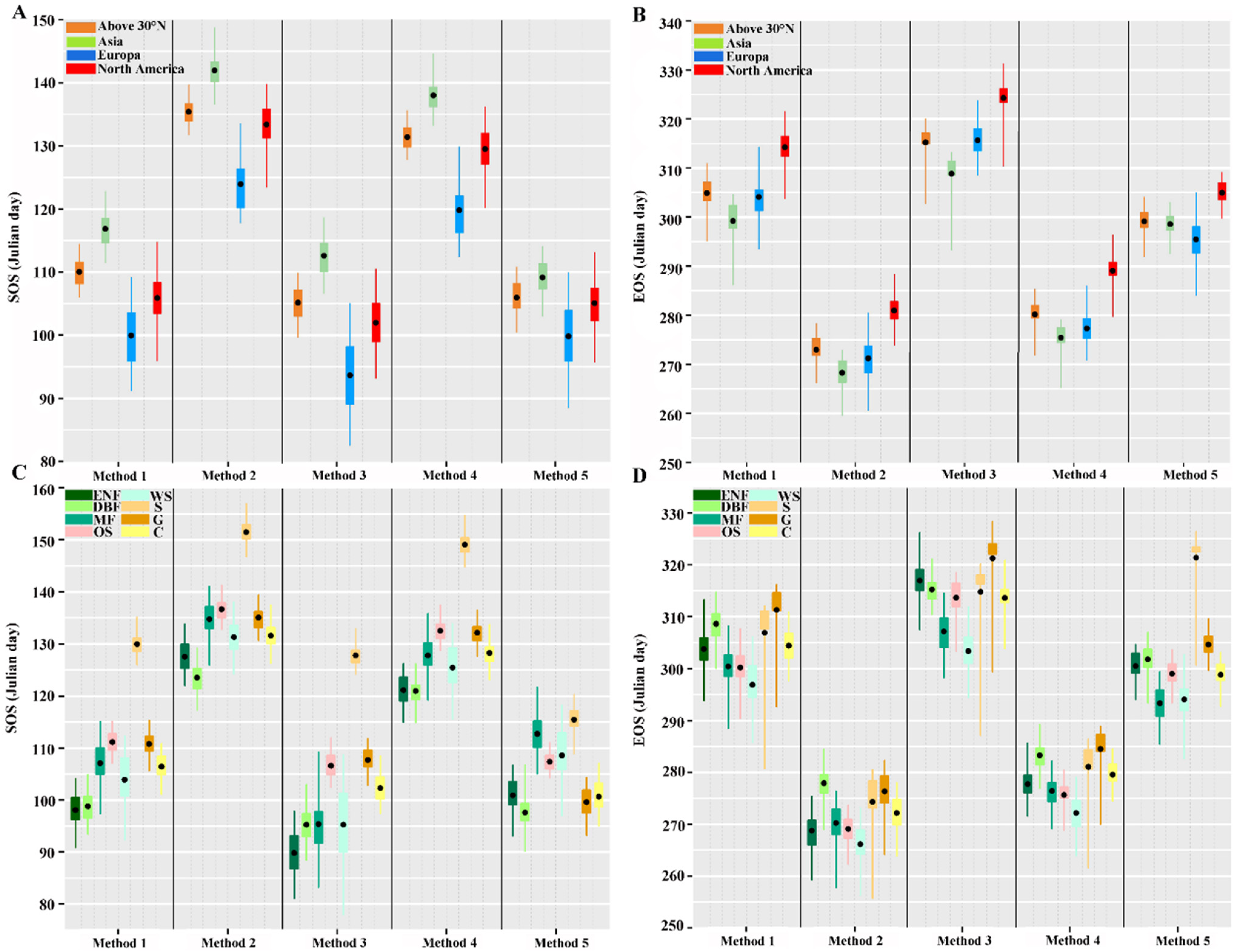
3.1. Consistency of Vegetation Phenology Parameters

The interannual changes of the SOS and EOS under the five methods have great differences above 30°N (Figure 3). For the SOS (Figure 3A), the variation ranges under Methods 1, 3 and 5 in each region were similar, and the value was mainly concentrated between 83 and 123 days. The variation ranges of the SOS under Methods 2 and 4 were similar, and the value was mainly concentrated between 113 and 148 days. By analysing the SOS under different vegetation types, we also found that it is the same as that in different regions, which shows that the SOS extracted using Methods 2 and 4 is obviously delayed by approximately 30 days compared with Methods 1, 3 and 5. This may be because the threshold limit of method 2 and method 4 on NDVI is obviously higher than that of the other methods, and the regions with low NDVI values are not extracted well, which leads to the lagging of the SOS. However, the changes of the SOS were consistent in different regions, showing that Europe < North America < above 30°N < Asia. For instance, for MF and WS (Figure 3C), the interannual variation of the SOS extracted using method 3 is obviously higher than that extracted using other methods. In addition, the interannual variation of the SOS under the five extraction methods is small.
For EOS (Figure 3B), the variation range in each region is larger under each method. The variation ranges of the EOS under Methods 2, 4 and 5 are roughly the same and are mostly concentrated from 260 to 309 days. However, the EOS under Methods 1 and 3 is in most cases delayed from 287 to 332 days. This may also be because the threshold limit of Methods 2 and 4 on the NDVI is obviously higher than that of other methods, and the regions with low NDVI values are not extracted well, which leads to the advancement of the EOS. Except for Method 5, the EOS average change across different regions is the same, showing that North America > above 30°N > Europe > Asia. However, judging from the EOS under different methods (Figure 3D), the interannual variation range of different vegetation types is large, among which S and G are the most obvious. However, the interannual variation range of the EOS under different vegetation types extracted using Methods 4 and 5 is obviously smaller than that extracted using other methods.

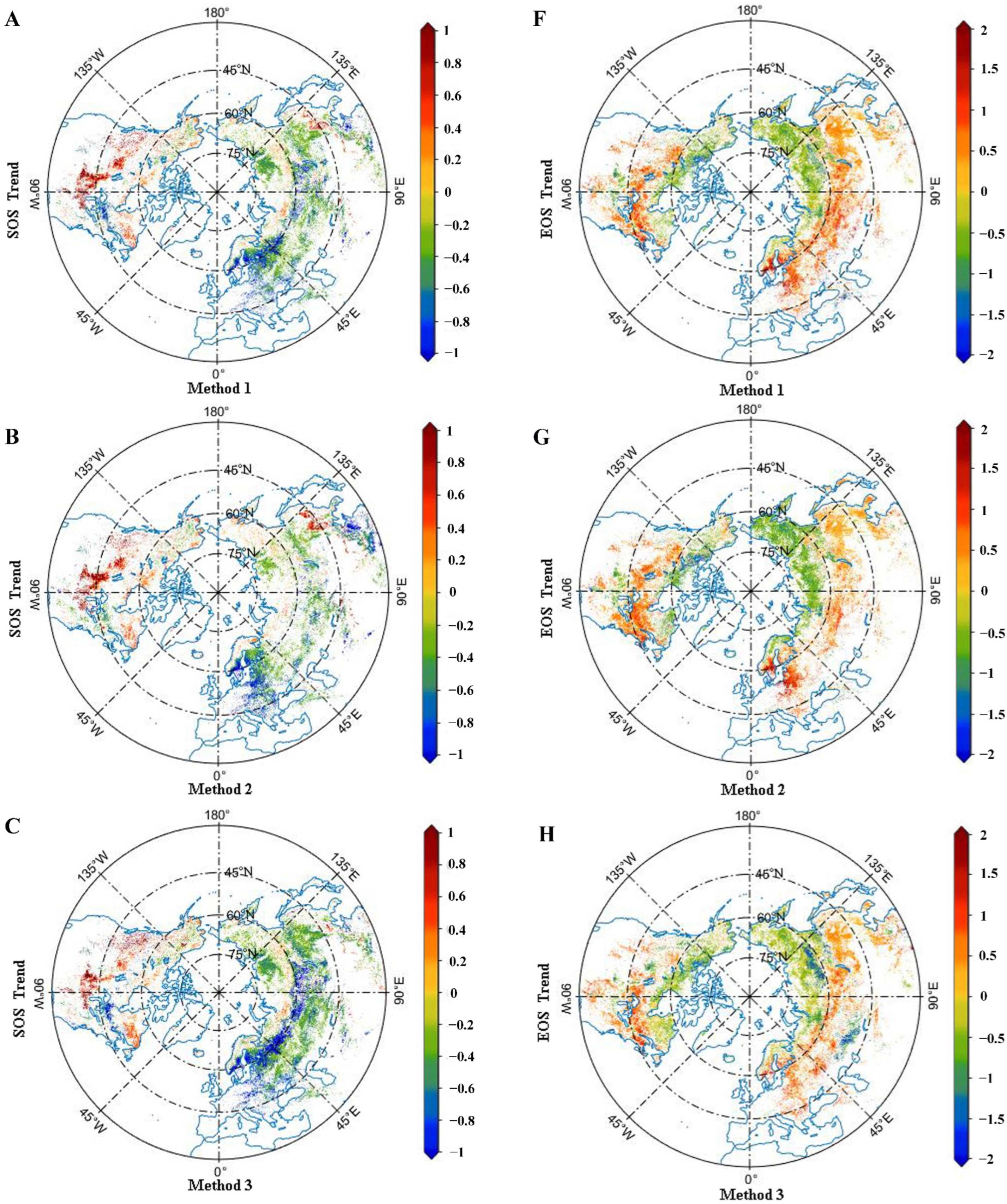
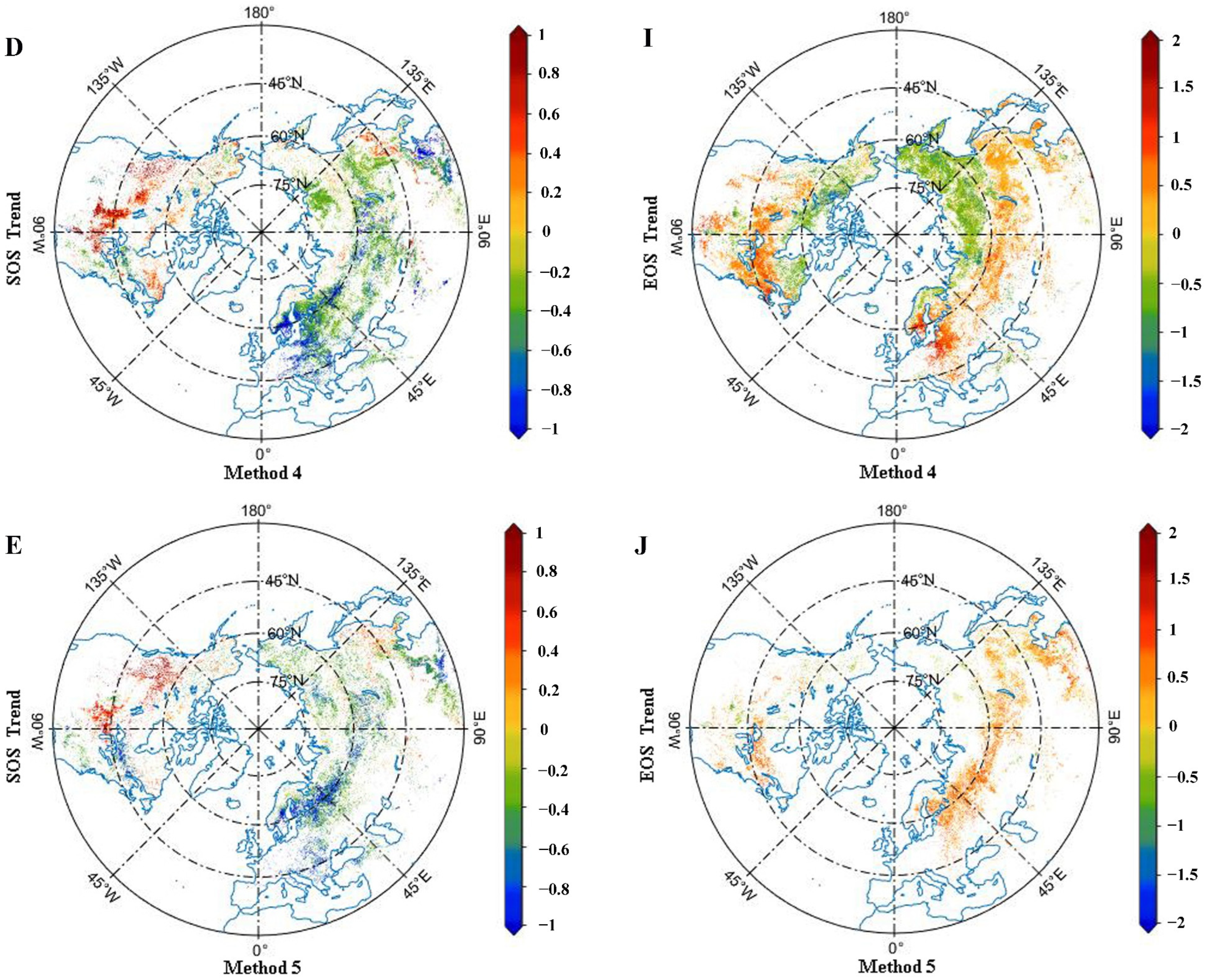
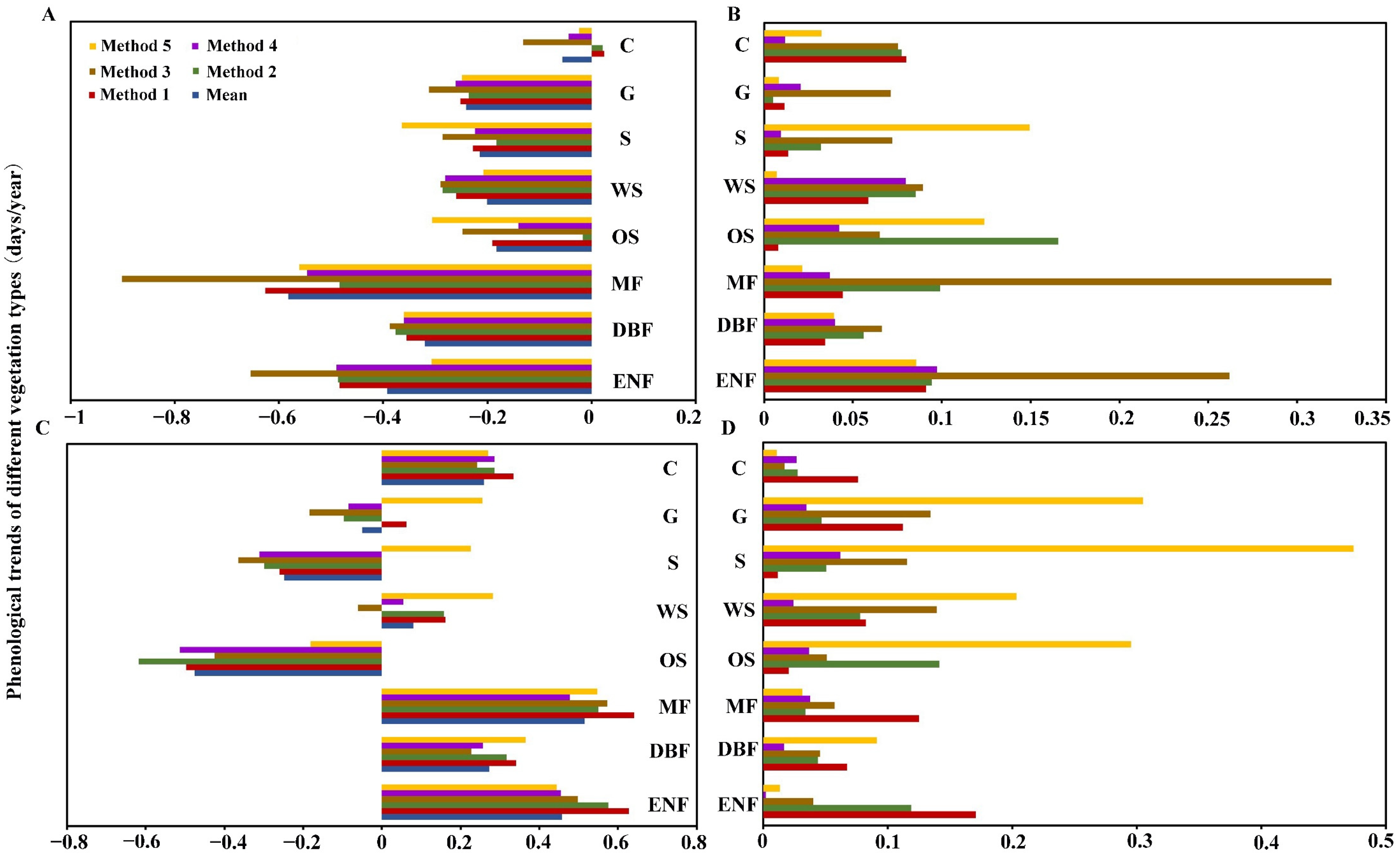
3.2. Consistency of Vegetation Phenology Trends

By analysing the SOS and EOS trends under the different methods above 30°N from 1982 to 2015, we found that the SOS trend was almost consistent under the five selected methods. There was a significant advancing trend (p < 0.05) for Methods 1–5 (Figure 4A–E). The number of pixels shows a significant advancing trend accounting for 73.12%, 68.35%, 75.10%, 72.62% and 73.88% of the total number of pixels, respectively. However, in some regions, the advancing trend under the five methods is also greatly different. For instance, in the Asian region between 30°N and 45°N, the SOS advancing trend for Methods 2 and 4 is significantly higher than that of the other three methods (Figure 4A–E and Table 1). For Asian and European regions between 45°N and 75°N, the SOS advancing trend for Methods 1,3 and 5 is significantly higher than that of Methods 2 and 4 (Figure 4A–E and Table 1). This may be because the SOS under the five selected methods is greatly influenced by vegetation type.
The variation law of the EOS under the five selected methods is basically consistent above 30°N. The EOS under the five methods mainly lags between 30°N and 60°N and advances between 60°N and 75°N (Figure 4F–J). However, there are also great differences in some regions. For Asia between 45°N and 60°N, the lagging trend and the number of significant pixels of the EOS in Method 1 are significantly higher than those of the other methods (Figure 4F–J and Table 2), and in Europe between 45°N and 60°N, the lagging trends in Methods 1 and 2 are significantly higher than in Methods 3, 4, and 5. However, in Asia and North America, there is a significant advancing trend from 60°N to 75°N. The advancing trend under Method 2 in Asia is especially obvious at 0.58 days/year (Table 2). Compared with other extraction methods, the advancing trend of the EOS under Method 5 is significantly lower than that under other methods, especially in North America.

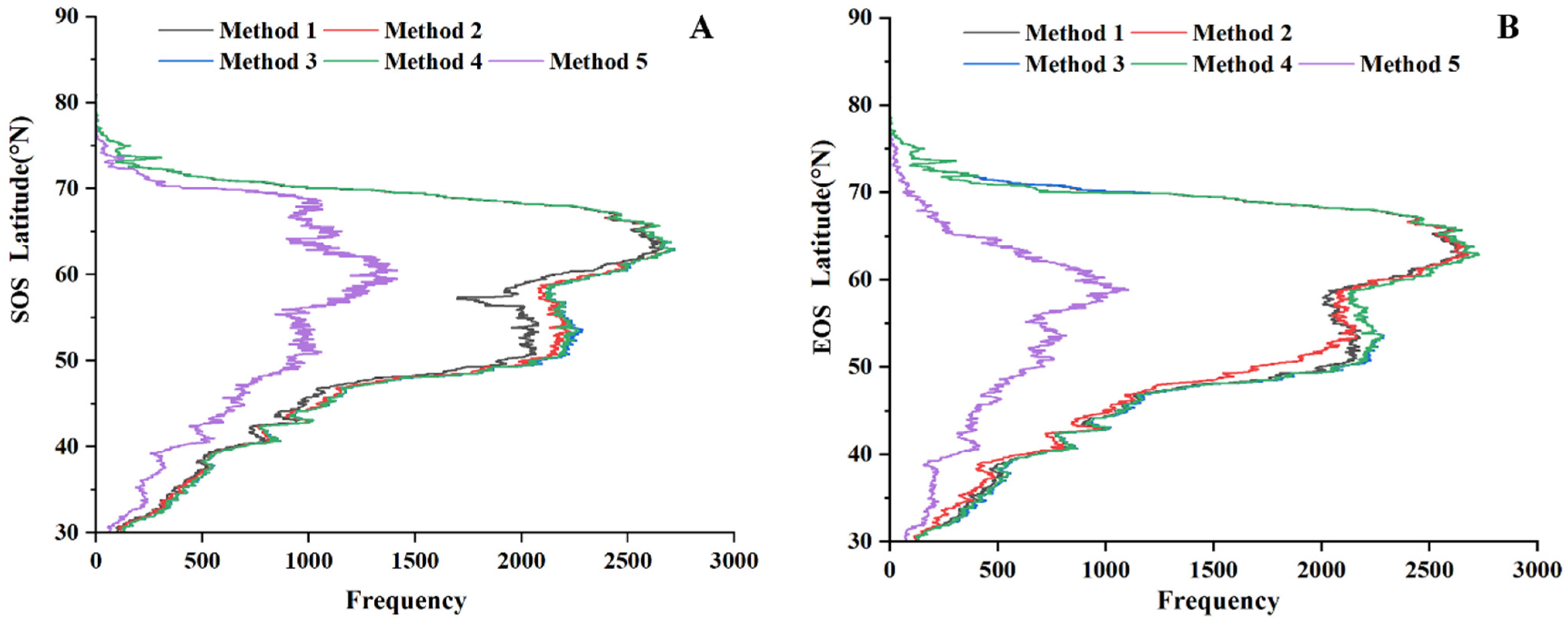
3.3. Consistency of Latitude Changes in Vegetation Phenology

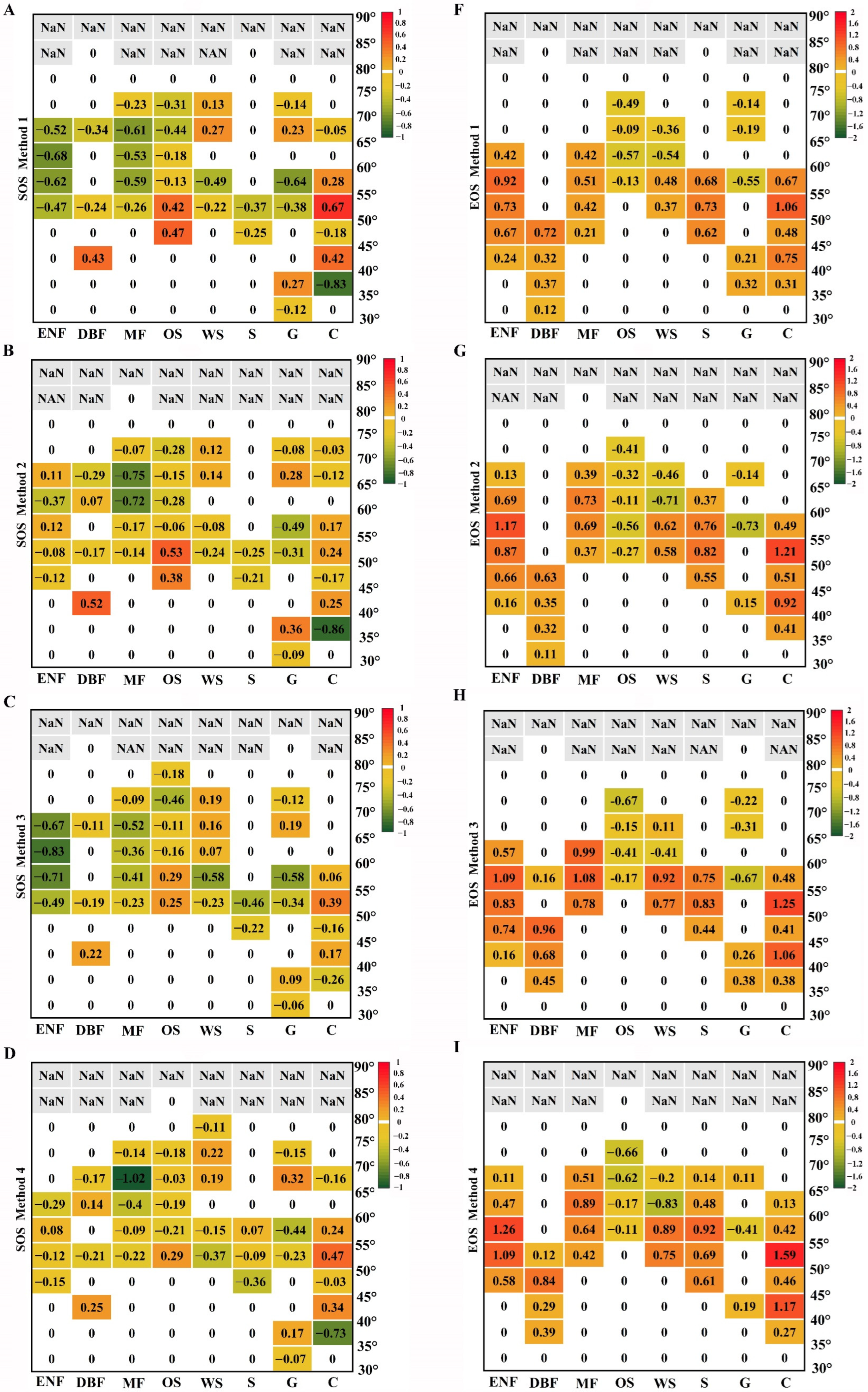
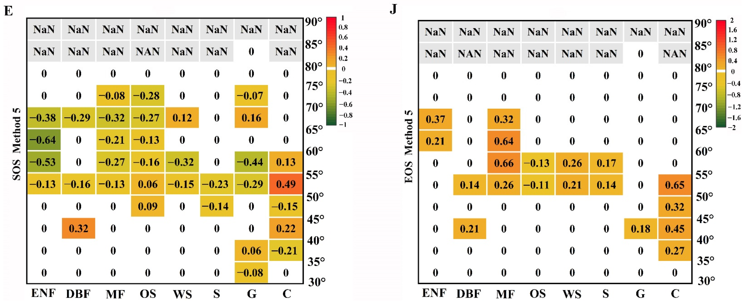
3.3.1. Significant Trends in Vegetation Phenology by Latitude

Studying significant trends in vegetation phenology reveals dynamic changes in vegetation. In this research, to analyse change trends according to latitude, we divided the region above 30°N into 0.083° latitude zones and calculated the number of significant phenology trends in each zone using the five above-stated methods (Figure 5). By analysing the SOS latitude changes under these methods (Figure 5A), we found that the curve variation law for the number of pixels with a significant trend was consistent under Methods 1 to 4, showing a strong increasing trend from low to high latitudes and a maximum value at approximately 65°N. However, far fewer pixels show a significant trend under Method 5, and the maximum number of pixels in latitudes appears earlier, at approximately 60°N.
Furthermore, under the same five methods, the significant number of SOS trends is mainly distributed between 50°N and 70°N, while the EOS curve change denoting the significant number of pixels in latitudes is very similar to the SOS (Figure 5B), except for Method 5. Under that method, the maximum number of pixels for EOS is earlier than for SOS and appears at approximately 58°N. Meanwhile, for all the five methods, the pixel distribution range of a significant EOS trend has increased and is mainly distributed between 45°N and 70°N.

3.3.2. Consistency of Phenological Trends of Different Vegetation Types by Latitude

Determining changes in vegetation phenology according to latitude is important for analysing trend differences using different methods. To analyse the various vegetation phenology trends above 30°N, the region between 30°N and 90°N is divided into latitude zones of 5° units. The phenological trends in different vegetation types in the pixels where the land cover types have not changed are then calculated (Figure 6). By analysing the SOS trend changes, we found that the advancing trend mostly dominated in different vegetation types according to latitude zone, with an advanced trend range of 0 to 0.86 days/year.
However, there are still some differences in the SOS under the various methods. For ENF, Methods 1 (Figure 6A), 3 (Figure 6C) and 5 (Figure 6E) show a significant advancing trend between 55°N and 70°N, while Methods 2 (Figure 6B) and 4 (Figure 6D) show no obvious trend. For DBF, the SOS shows a different delay trend under different methods at 40°~45°N. For MF, the variation law of different methods is the same in the latitude zone, showing an advancing trend at 50°~75°N that is most significant at 65°~70°N. The maximum advancing trend can reach 1.02 days/year. For other vegetation types, the SOS trend varies by latitude.
For the EOS under the five tested methods, the ENF change is consistent, showing a delaying trend between 45°N and 65°N. Specifically, Methods 1 (Figure 6F), 2 (Figure 6G), 3 (Figure 6H) and 4 (Figure 6I) all show maximum delaying trends of 0.92, 1.17, 1.09, and 1.26 days/year, respectively, between 55°N and 60°N. For DBF and MF, the delaying trend under Methods 1 and 2 is smaller than Methods 3 and 4 in the corresponding latitude zones. For OS, the EOS trends are advanced in the corresponding latitudes for Methods 1 to 4, between 70°N and 75°N. For C, the EOS trends for all five methods are lagged at 35°~55°N, and the maximum delay appears at 50°~55°N. For Methods 1–5, the delay trends are 1.06, 1.21, 1.25, 1.59, and 0.65 days/year, respectively.
According to the analysis of phenological trends of different vegetation types under the five chosen extraction methods (Figure 7A), the SOS trends of other vegetation are all consistent (except for C) and show an advancing trend, among which MF and ENF are more advanced than other vegetations. However, there are significant differences (p < 0.05) between MF and ENF under the different extraction methods (Table 3). By comparing the SOS trend average of the five extraction methods (Figure 7B), we found that Method 4 was the most suitable for SOS extraction of C and S, and Method 5 was the most suitable for SOS extraction of WS and MF. Additionally, Method 1 is the most suitable for SOS extraction of OS and DBF. Except for Method 5, all methods are suitable for SOS extraction of ENF.
For the EOS trends of different vegetation types (Figure 7C), the trends of G, S and OS are mainly advancing under the different extraction methods, while those of other vegetation are mainly delaying. By comparing the EOS trend average of the five extraction methods (Figure 7D), we found that, for C and MF, Method 5 was the best method for EOS extraction, but it was the worst for G, S, WS, and OS. Moreover, for G and DBF, Method 4 is the best approach for EOS extraction, and Method 1 is the best for EOS extraction of S and OS.

3.4. Phenological Consistency between Remote Sensing and Ground Data

To study the similarities and differences between remote sensing data and ground data in vegetation phenology above 30°N, we employed the same five methods used above, extracted the phenological data from weekly mean GPP data from 25 qualified flux towers and applied the average value as ground phenological parameters.
Based on the SOS analysis from the image data and ground data (Table 4), we found that the SOS from the image data and ground data under different methods above 30°N were significantly correlated (p < 0.05); however, according to the correlation coefficients (R) and the root mean square error (RMSE), we found that Method 3 had a higher R (0.94, p < 0.05) and the lowest RMSE (4.35) than the other methods, and was most suitable for the extraction of the SOS in this area. However, for different latitude regions, the phenological consistency between remote sensing data and ground data is greatly different under different extraction methods. From the R and RMSE, we found that Methods 2 and 4 are more suitable for the extraction of the SOS from 30°N to 45°N, and Methods 3 and 5 are more suitable for the extraction of the SOS from 45°N to 75°N.
By analysing the consistency of the EOS between image data and ground data above 30°N (Table 5), we found that Method 4 has the highest significant correlation coefficient (0.83, p < 0.05) and the lowest RMSE (7.49) compared to the other methods, and is most suitable for the extraction of the EOS in this area. For 30°N to 45°N and 60°N to 75°N, compared with other methods, Methods 3 and 4 have higher significant correlation coefficient and lower RMSE, making them more suitable for the extraction of the EOS in these regions. Method 4 has the highest correlation coefficient (0.73) and the lowest RMSE (5.36) compared to the other methods from 45°N to 60°N, thus it is most suitable for the extraction of EOS in this region.

4. Discussion

Using an appropriate algorithm for phenological parameters extraction from remote sensing images of a time series is a key step in applying remote sensing phenology to modelling [41,42,43]. To study the dynamic change of vegetation growth more accurately, additional variables are constantly added to the SOS and EOS extraction methods, which makes the extraction of vegetation phenological parameters more complex [44].

4.1. Consistency of Characteristics and Trends in Vegetation Phenology

By analysing the characteristics of phenological parameters under different extraction methods, we found that there were great differences in the SOS and EOS. Specifically, the average of the SOS extracted under Methods 1, 3, and 5 was obviously earlier than Methods 2 and 4, and the average of the EOS under Methods 1 and 3 was significantly later than Methods 2 and 4 in different regions and vegetation types (Figure 3). This is mainly because the mechanism of different extraction methods is different. Compared with the other methods, Methods 2 and 4 have higher requirements for the NDVI threshold and do not identify some vegetation with an earlier growing season and smaller NDVI, so the SOS is obviously later than that of other methods, and the EOS is obviously earlier than that of the other methods.
The trend of vegetation phenological parameters is a crucial indicator affecting vegetation phenology. In our study, we found that the spatial distribution of the SOS and the five methods were consistent, showing an advancing trend, which is the same as the results obtained by Zhang et al. for vegetation phenology in the Northern Hemisphere [15]. However, the SOS trends under the five selected methods differed in some regions, especially in Asia and Europe between 45°N and 60°N. This may be due to the different responses of different vegetation types to hydrothermal conditions. Because in Asia between 45°N and 55°N, the main vegetation is G, mainly distributed in the arid areas [45], the water stress will significantly affect the dynamic changes in NDVI in this region [46], and lead to significant differences in trend of the SOS under different extraction methods. Temperature has been widely recognised as the dominant climatic variable driving changes in vegetation phenology for temperate and boreal ecosystems across the Northern Hemisphere [31,47,48]. Furthermore, for the Asian and European regions between 55°N and 60°N, the main vegetation is MF, which is a mixture of various tree species. Due to the different responses of various trees to temperature [49], increases in temperature will lead to large fluctuations in the composition of vegetation in this region and aggravate the inconsistency of vegetation phenology under different extraction methods [8,31,50].
For the trend of the EOS, most areas from 30°N to 60°N show a lagging trend under the five selected methods, which is the same as the results obtained by Zhang et al. [15]. However, the EOS trend under Method 5 above 60°N is significantly different from that under the other extraction methods. This may be because Method 5 has poor NDVI recognition for the OS in this region, which affects the trend. Therefore, when studying the change in the EOS in this region, the deficiency of this method should be considered.

4.2. Consistency of Latitude Variation in Vegetation Phenology

When phenology extraction is based on remote sensing image data, the differences in the extraction methods used are one of the main reasons for the change in accuracy [19], as individual regions have different spatial heterogeneity changes in phenology. Therefore, studying similarities and differences in vegetation phenology under a variety of extraction methods and latitudes plays an important role in accurately extracting regional phenology parameters [15,48,49].
We found that the number of pixels under the five extraction methods was relatively small above 80°N, making it difficult to evaluate the phenological trend in these regions. The SOS of different vegetation types under the five methods used in this study shows an advancing trend at different latitudes. Among them, the advancing trend of the SOS is more significant between 50°N and 70°N (p < 0.05), likely due to spring advancements being more significant in the mid-high latitudes [1,24,51,52]. However, the SOS differs according to latitude. This may be because different vegetation types affect the SOS of the five extraction methods (Figure 6). Moreover, for most land cover types, the EOS shows mainly a delayed trend from 30°N to 60°N, which is the same as Zhang et al.’s results [15]. However, other than for Method 5, the vegetation phenological trend above 60°N is primarily an advancing trend, which is consistent with Zeng et al.’s finding [2]. The dissimilarities in these results may be due to the use of different image datasets and time periods [41,53]. Therefore, when extracting vegetation phenological parameters in the future, the effects of different vegetation types on the extraction methods should be fully considered (Figure 7), and the appropriate extraction methods should be selected according to the characteristics of the study area.

4.3. Phenological Consistency between Remote Sensing and Ground

Numerous scholars working in the phenology field have used double logistic function to fit the curve of GPP [32,54], so we also used this method to fit the weekly mean GPP. We consider the phenology extracted of GPP under the five selected methods as real values to test the phenological results using image data extraction. To improve the consistency of phenological parameters between remote sensing and ground data, we should adopt suitable extraction methods at different latitudes. We found that Method 3 was most suitable for the extraction of the SOS above 30°N, Methods 2 and 4 were more suitable for the extraction of the SOS from 30°N to 45°N, and Methods 3 and 5 were more suitable for the extraction of the SOS from 45°N to 75°N. For EOS, Method 4 is most suitable for the extraction of the EOS above 30°N, and for 30°N to 45°N and 60°N to 75°N, Methods 3 and 4 are more suitable, respectively. The differences in the above results may be caused by changes in vegetation types and climate factors. However, we select fewer ground stations, which may also affect the accuracy of the verification results.

5. Shortcomings and Future Works

In this paper, we evaluated the consistency of vegetation phenological parameters under different extraction methods of the same fitting function applied to Northern Hemisphere in 1982–2015 based on the GIMMS3g dataset, but there are still some areas that need to be further explored in-depth. When using different methods to extract vegetation phenological parameters, the effects of water stress on vegetation photosynthesis are not considered, especially in arid ecosystem, which may also lead to the uncertainty of phenological parameters. The spatial resolution of the GIMMS3g NDVI dataset is lower than that of the land cover dataset, which will lead to inaccurate phenological results for different vegetation types after resampling. Furthermore, the period of the GIMMS3g NDVI dataset is only from 1982 to 2015, and we will integrate a series of products over a longer time and at a higher resolution to further discuss the consistency of vegetation phenological parameters under different extraction methods in future studies.

6. Conclusions

We used double logistic functions to fit the curve for GIMMS3g NDVI and selected five commonly employed methods to extract the phenological parameters above 30°N during 1982–2015. We found that the spatial distribution and trends of the SOS and EOS under the chosen extraction methods had both similarities and differences. Furthermore, we found that through the verification of flux data, the SOS extracted using Method 3 from the GIMMS3g dataset was the closest to the ground data, while the EOS extracted using Method 4 was the closest to the ground data.
Overall, regardless of the method employed, the average changes in phenological parameters were consistent during the study period, with the SOS showing Asia > whole > North America > Europe, while the EOS showed North America > whole > Europe > Asia. However, the SOS under Methods 1, 3 and 5 was significantly earlier than that under Methods 2 and 4, while the EOS under methods 1 and 3 was notably later than that under Methods 2 and 4.
Regarding phenological parameters, the SOS trends under the five methods mostly showed an advance, except for the SOS trends from 45°N to 60°N in Asia and Europe. The EOS trends, on the other hand, showed a clear lag under Methods 1 to 4 from 30°N to 60°N and an advance above 60°N. In addition to the above dissimilarities, vegetation type was also shown to be a notable factor influencing the extraction of phenological parameters above 30°N.

Author Contributions

Conceptualization, X.L. and Y.C.; methodology, Y.C.; validation, X.L., Y.L. and Z.L.; writing—original draft preparation, X.L.; writing—review and editing, X.L., Y.L. and Y.C.; funding acquisition, Z.L. All authors have read and agreed to the published version of the manuscript.

Funding

This research was funded by the National Key Research and Development Program, 2019YFA0606902.

Data Availability Statement

The data presented in this study are available on request from the corresponding author.

Conflicts of Interest

The authors declare no conflict of interest.

References

  1. Jeganathan, C.; Dash, J.; Atkinson, P. Remotely sensed trends in the phenology of northern high latitude terrestrial vegetation, controlling for land cover change and vegetation type. Remote Sens. Environ. 2014, 143, 154–170. [Google Scholar] [CrossRef]
  2. Zeng, H.; Jia, G.; Epstein, H. Recent changes in phenology over the northern high latitudes detected from multi-satellite data. Environ. Res. Lett. 2011, 6, 045508. [Google Scholar] [CrossRef]
  3. Jeong, S.J.; Ho, C.H.; Gim, H.J.; Brown, M.E. Phenology shifts at start vs. end of growing season in temperate vegetation over the Northern Hemisphere for the period 1982–2008. Glob. Chang. Biol. 2011, 17, 2385–2399. [Google Scholar] [CrossRef]
  4. Jeong, S.J.; Ho, C.H.; Kim, K.Y.; Jeong, J.H. Reduction of spring warming over East Asia associated with vegetation feedback. Geophys. Res. Lett. 2009, 36, 9114. [Google Scholar] [CrossRef]
  5. Barr, A.; Black, T.A.; McCaughey, H. Climatic and phenological controls of the carbon and energy balances of three contrasting boreal forest ecosystems in western Canada. In Phenology of Ecosystem Processes; Springer: Cham, Switzerland, 2009; pp. 3–34. [Google Scholar] [CrossRef]
  6. Heumann, B.W.; Seaquist, J.; Eklundh, L.; Jönsson, P. AVHRR derived phenological change in the Sahel and Soudan, Africa, 1982–2005. Remote Sens. Environ. 2007, 108, 385–392. [Google Scholar] [CrossRef]
  7. Wang, J.; Zhang, X. Investigation of wildfire impacts on land surface phenology from MODIS time series in the western US forests. ISPRS J. Photogramm. Remote Sens. 2020, 159, 281–295. [Google Scholar] [CrossRef]
  8. Shen, M.; Zhang, G.; Cong, N.; Wang, S.; Kong, W.; Piao, S. Increasing altitudinal gradient of spring vegetation phenology during the last decade on the Qinghai–Tibetan Plateau. Agric. For. Meteorol. 2014, 189, 71–80. [Google Scholar] [CrossRef]
  9. Delbart, N.; Kergoat, L.; Le Toan, T.; Lhermitte, J.; Picard, G. Determination of phenological dates in boreal regions using normalized difference water index. Remote Sens. Environ. 2005, 97, 26–38. [Google Scholar] [CrossRef]
  10. Verbesselt, J.; Hyndman, R.; Zeileis, A.; Culvenor, D. Phenological change detection while accounting for abrupt and gradual trends in satellite image time series. Remote Sens. Environ. 2010, 114, 2970–2980. [Google Scholar] [CrossRef]
  11. Ganguly, S.; Friedl, M.A.; Tan, B.; Zhang, X.; Verma, M. Land surface phenology from MODIS: Characterization of the Collection 5 global land cover dynamics product. Remote Sens. Environ. 2010, 114, 1805–1816. [Google Scholar] [CrossRef]
  12. Vrieling, A.; Meroni, M.; Darvishzadeh, R.; Skidmore, A.K.; Wang, T.; Zurita-Milla, R.; Oosterbeek, K.; O’Connor, B.; Paganini, M. Vegetation phenology from Sentinel-2 and field cameras for a Dutch barrier island. Remote Sens. Environ. 2018, 215, 517–529. [Google Scholar] [CrossRef]
  13. Zipper, S.C.; Schatz, J.; Singh, A.; Kucharik, C.J.; Townsend, P.A.; Loheide, S.P. Urban heat island impacts on plant phenology: Intra-urban variability and response to land cover. Environ. Res. Lett. 2016, 11, 054023. [Google Scholar] [CrossRef]
  14. Walker, J.; De Beurs, K.; Wynne, R. Dryland vegetation phenology across an elevation gradient in Arizona, USA, investigated with fused MODIS and Landsat data. Remote Sens. Environ. 2014, 144, 85–97. [Google Scholar] [CrossRef]
  15. Zhang, J.; Zhao, J.; Wang, Y.; Zhang, H.; Zhang, Z.; Guo, X. Comparison of land surface phenology in the Northern Hemisphere based on AVHRR GIMMS3g and MODIS datasets. ISPRS J. Photogramm. Remote Sens. 2020, 169, 1–16. [Google Scholar] [CrossRef]
  16. Yuan, H.; Wu, C.; Lu, L.; Wang, X. A new algorithm predicting the end of growth at five evergreen conifer forests based on nighttime temperature and the enhanced vegetation index. ISPRS J. Photogramm. Remote Sens. 2018, 144, 390–399. [Google Scholar] [CrossRef]
  17. Liu, Y.; Hill, M.J.; Zhang, X.; Wang, Z.; Richardson, A.D.; Hufkens, K.; Filippa, G.; Baldocchi, D.D.; Ma, S.; Verfaillie, J. Using data from Landsat, MODIS, VIIRS and PhenoCams to monitor the phenology of California oak/grass savanna and open grassland across spatial scales. Agric. For. Meteorol. 2017, 237, 311–325. [Google Scholar] [CrossRef]
  18. Garonna, I.; de Jong, R.; Schaepman, M.E. Variability and evolution of global land surface phenology over the past three decades (1982–2012). Glob. Chang. Biol. 2016, 22, 1456–1468. [Google Scholar] [CrossRef] [PubMed]
  19. Zhang, X. Reconstruction of a complete global time series of daily vegetation index trajectory from long-term AVHRR data. Remote Sens. Environ. 2015, 156, 457–472. [Google Scholar] [CrossRef]
  20. Beck, P.S.; Atzberger, C.; Høgda, K.A.; Johansen, B.; Skidmore, A.K. Improved monitoring of vegetation dynamics at very high latitudes: A new method using MODIS NDVI. Remote Sens. Environ. 2006, 100, 321–334. [Google Scholar] [CrossRef]
  21. Jonsson, P.; Eklundh, L. Seasonality extraction by function fitting to time-series of satellite sensor data. IEEE Trans. Geosci. Remote Sens. 2002, 40, 1824–1832. [Google Scholar] [CrossRef]
  22. Beaubien, E.; Freeland, H. Spring phenology trends in Alberta, Canada: Links to ocean temperature. Int. J. Biometeorol. 2000, 44, 53–59. [Google Scholar] [CrossRef] [PubMed]
  23. Savitzky, A.; Golay, M.J. Smoothing and differentiation of data by simplified least squares procedures. Anal. Chem. 1964, 36, 1627–1639. [Google Scholar] [CrossRef]
  24. Piao, S.; Fang, J.; Zhou, L.; Ciais, P.; Zhu, B. Variations in satellite-derived phenology in China’s temperate vegetation. Glob. Chang. Biol. 2006, 12, 672–685. [Google Scholar] [CrossRef]
  25. White, M.A.; Thornton, P.E.; Running, S.W. A continental phenology model for monitoring vegetation responses to interannual climatic variability. Glob. Biogeochem. Cycles. 1997, 11, 217–234. [Google Scholar] [CrossRef]
  26. Kaduk, J.; Heimann, M. A prognostic phenology scheme for global terrestrial carbon cycle models. Clim. Res. 1996, 6, 1–19. [Google Scholar] [CrossRef]
  27. Fischer, A. A model for the seasonal variations of vegetation indices in coarse resolution data and its inversion to extract crop parameters. Remote Sens. Environ. 1994, 48, 220–230. [Google Scholar] [CrossRef]
  28. Zeng, Z.; Wu, W.; Ge, Q.; Li, Z.; Wang, X.; Zhou, Y.; Zhang, Z.; Li, Y.; Huang, H.; Liu, G. Legacy effects of spring phenology on vegetation growth under preseason meteorological drought in the Northern Hemisphere. Agric. For. Meteorol. 2021, 310, 108630. [Google Scholar] [CrossRef]
  29. Wang, X.; Xiao, J.; Li, X.; Cheng, G.; Ma, M.; Zhu, G.; Altaf Arain, M.; Andrew Black, T.; Jassal, R.S. No trends in spring and autumn phenology during the global warming hiatus. Nat. Commun. 2019, 10, 2389. [Google Scholar] [CrossRef]
  30. Peng, J.; Wu, C.; Zhang, X.; Wang, X.; Gonsamo, A. Satellite detection of cumulative and lagged effects of drought on autumn leaf senescence over the Northern Hemisphere. Glob. Chang. Biol. 2019, 25, 2174–2188. [Google Scholar] [CrossRef] [PubMed]
  31. Piao, S.; Liu, Q.; Chen, A.; Janssens, I.A.; Fu, Y.; Dai, J.; Liu, L.; Lian, X.; Shen, M.; Zhu, X. Plant phenology and global climate change: Current progresses and challenges. Glob. Chang. Biol. 2019, 25, 1922–1940. [Google Scholar] [CrossRef]
  32. Chang, Q.; Xiao, X.; Jiao, W.; Wu, X.; Doughty, R.; Wang, J.; Du, L.; Zou, Z.; Qin, Y. Assessing consistency of spring phenology of snow-covered forests as estimated by vegetation indices, gross primary production, and solar-induced chlorophyll fluorescence. Agric. For. Meteorol. 2019, 275, 305–316. [Google Scholar] [CrossRef]
  33. Julien, Y.; Sobrino, J. Global land surface phenology trends from GIMMS database. Int. J. Remote Sens. 2009, 30, 3495–3513. [Google Scholar] [CrossRef]
  34. Zhang, X.; Friedl, M.A.; Schaaf, C.B.; Strahler, A.H.; Hodges, J.C.; Gao, F.; Reed, B.C.; Huete, A. Monitoring vegetation phenology using MODIS. Remote Sens. Environ. 2003, 84, 471–475. [Google Scholar] [CrossRef]
  35. Studer, S.; Stöckli, R.; Appenzeller, C.; Vidale, P.L. A comparative study of satellite and ground-based phenology. Int. J. Biometeorol. 2007, 51, 405–414. [Google Scholar] [CrossRef] [PubMed]
  36. Yu, H.; Luedeling, E.; Xu, J. Winter and spring warming result in delayed spring phenology on the Tibetan Plateau. Proc. Natl. Acad. Sci. USA 2010, 107, 22151–22156. [Google Scholar] [CrossRef]
  37. Reed, B.C.; Brown, J.F.; VanderZee, D.; Loveland, T.R.; Merchant, J.W.; Ohlen, D.O. Measuring phenological variability from satellite imagery. J. Veg. Sci. 1994, 5, 703–714. [Google Scholar] [CrossRef]
  38. Wang, T.; Peng, S.; Lin, X.; Chang, J. Declining snow cover may affect spring phenological trend on the Tibetan Plateau. Proc. Natl. Acad. Sci. USA 2013, 110, E2854–E2855. [Google Scholar] [CrossRef]
  39. Theil, H. A rank-invariant method of linear and polynomial regression analysis. In Henri Theil’s Contributions to Economics and Econometrics: Econometric Theory and Methodology; Springer: Cham, Switzerland, 1992; pp. 345–381. [Google Scholar]
  40. Mann, H.B. Nonparametric tests against trend. Econometrica 1945, 13, 245–259. [Google Scholar] [CrossRef]
  41. Kandasamy, S.; Fernandes, R. An approach for evaluating the impact of gaps and measurement errors on satellite land surface phenology algorithms: Application to 20 year NOAA AVHRR data over Canada. Remote Sens. Environ. 2015, 164, 114–129. [Google Scholar] [CrossRef]
  42. Cao, R.; Chen, J.; Shen, M.; Tang, Y. An improved logistic method for detecting spring vegetation phenology in grasslands from MODIS EVI time-series data. Agric. For. Meteorol. 2015, 200, 9–20. [Google Scholar] [CrossRef]
  43. Garrity, S.R.; Bohrer, G.; Maurer, K.D.; Mueller, K.L.; Vogel, C.S.; Curtis, P.S. A comparison of multiple phenology data sources for estimating seasonal transitions in deciduous forest carbon exchange. Agric. For. Meteorol. 2011, 151, 1741–1752. [Google Scholar] [CrossRef]
  44. Wu, C.; Peng, D.; Soudani, K.; Siebicke, L.; Gough, C.M.; Arain, M.A.; Bohrer, G.; Lafleur, P.M.; Peichl, M.; Gonsamo, A. Land surface phenology derived from normalized difference vegetation index (NDVI) at global FLUXNET sites. Agric. For. Meteorol. 2017, 233, 171–182. [Google Scholar] [CrossRef]
  45. Prăvălie, R.; Bandoc, G.; Patriche, C.; Sternberg, T. Recent changes in global drylands: Evidences from two major aridity databases. CATENA 2019, 178, 209–231. [Google Scholar] [CrossRef]
  46. Xu, X. Global patterns and ecological implications of diurnal hysteretic response of ecosystem water consumption to vapor pressure deficit. Agric. For. Meteorol. 2022, 314, 108785. [Google Scholar] [CrossRef]
  47. Gao, M.; Wang, X.; Meng, F.; Liu, Q.; Li, X.; Zhang, Y.; Piao, S. Three-dimensional change in temperature sensitivity of northern vegetation phenology. Glob. Chang. Biol. 2020, 26, 5189–5201. [Google Scholar] [CrossRef]
  48. Peng, D.; Zhang, X.; Zhang, B.; Liu, L.; Liu, X.; Huete, A.R.; Huang, W.; Wang, S.; Luo, S.; Zhang, X. Scaling effects on spring phenology detections from MODIS data at multiple spatial resolutions over the contiguous United States. ISPRS J. Photogramm. Remote Sens. 2017, 132, 185–198. [Google Scholar] [CrossRef]
  49. O’Connor, B.; Dwyer, E.; Cawkwell, F.; Eklundh, L. Spatio-temporal patterns in vegetation start of season across the island of Ireland using the MERIS Global Vegetation Index. ISPRS J. Photogramm. Remote Sens. 2012, 68, 79–94. [Google Scholar] [CrossRef]
  50. Ogutu, J.O.; Owen-Smith, N.; Piepho, H.-P.; Kuloba, B.; Edebe, J. Dynamics of ungulates in relation to climatic and land use changes in an insularized African savanna ecosystem. Biodivers. Conserv. 2012, 21, 1033–1053. [Google Scholar] [CrossRef]
  51. Wang, X.; Piao, S.; Xu, X.; Ciais, P.; MacBean, N.; Myneni, R.B.; Li, L. Has the advancing onset of spring vegetation green-up slowed down or changed abruptly over the last three decades? Glob. Ecol. Biogeogr. 2015, 24, 621–631. [Google Scholar] [CrossRef]
  52. Zhang, G.; Zhang, Y.; Dong, J.; Xiao, X. Green-up dates in the Tibetan Plateau have continuously advanced from 1982 to 2011. Proc. Natl. Acad. Sci. USA 2013, 110, 4309–4314. [Google Scholar] [CrossRef]
  53. Zhao, J.; Zhang, H.; Zhang, Z.; Guo, X.; Li, X.; Chen, C. Spatial and temporal changes in vegetation phenology at middle and high latitudes of the Northern Hemisphere over the past three decades. Remote Sens. 2015, 7, 10973–10995. [Google Scholar] [CrossRef]
  54. Gonsamo, A.; Chen, J.M.; D’Odorico, P. Deriving land surface phenology indicators from CO2 eddy covariance measurements. Ecol. Indic. 2013, 29, 203–207. [Google Scholar] [CrossRef]
Figure 1. Comparison of phenological parameters under five extraction methods. The figure is the result of using five extraction methods to extract the SOS and EOS of a grid point (57.5°~57.583°E, 60.833°~60.917°N) in 2000. (AE) represent the five extraction methods. The black dots in the figure represent the NDVI values of 12 months in 2000, and the black lines represent the fitting results of double logistic functions, and the dotted lines represent the results of extracting the SOS and EOS by applying five extraction methods, respectively, and the details of the five extraction methods have been introduced in Section 2.3.
Remotesensing 15 02559 g001
Figure 2. Distribution of land types above 30°N from 2000 to 2015. The black dots represent the distribution of Flux2015 stations.
Remotesensing 15 02559 g002
Figure 3. Vegetation phenological changes above 30°N from 1982 to 2015. (A,B) represent the interannual changes of the SOS and EOS in different regions, respectively. (C,D) represent the interannual changes of the SOS and EOS in different vegetation types, respectively. The length of the box represents the interannual variation range of the SOS and EOS, and the shorter the box, the smaller the fluctuation of the data, and the longer the box, the greater the fluctuation of the data. Among them, the black dot in the middle of the box represents the average value of the data, the top of the whisker in the box represents the maximum value of the data, and the bottom of the whisker in the box represents the minimum value of the data.
Remotesensing 15 02559 g003
Figure 4. Phenological trend changes under different methods at mid and high latitudes. The trend changes under different extraction methods in the figure are all using the Theil-Sen method, and the Mann–Kendall method is used to test the trend. (AE) represent the SOS trend under Method 1, Method 2, Method 3, Method 4 and Method 5 at mid and high latitudes in the Northern Hemisphere, respectively. (FJ) represent the EOS trend under Methods 1–5 at mid and high latitudes in the Northern Hemisphere, respectively. The histogram in the lower left represents the percentage of positive trend and negative trend pixels in the total pixels under MK test, and different colours represent different trend range, all corresponding to the colour bands on the right.
Remotesensing 15 02559 g004aRemotesensing 15 02559 g004b
Figure 5. Pixel changes of significant phenological trends under different methods. (A,B), respectively represent the number of pixels of the SOS and EOS under different methods in latitudes, and different colours represent corresponding methods.
Remotesensing 15 02559 g005
Figure 6. Phenological trends in different vegetation types above 30°N. The values are the trend averages of the total pixels for different vegetation types in the corresponding latitudes. (AE) represent the SOS trend and (FJ) represent the EOS trend. The NaN indicates that there are missing values in this area. “0” represents the trend has not changed. ENF, DBF, MF, OS, WS, S, G and C on the abscissa represent different vegetation types, and are Evergreen Needleleaf Forests (ENF), Deciduous Broadleaf Forests (DBF), Mixed Forests (MF), Open Shrublands (OS), Woody Savannas (WS), Savannas (S), Grasslands (G), Croplands (C), respectively, different colours represent the trend change. All the trend values indicate an increase or decrease at a significant level of 95% (p < 0.05).
Remotesensing 15 02559 g006aRemotesensing 15 02559 g006b
Figure 7. Phenological trends of different vegetation types. (A,C) respectively represent the trend of SOS and EOS of different extraction methods under different vegetation types above 30°N. Among them, different colours represent different extraction methods, and blue represents the average of five extraction methods. (B,D), respectively represent the trend of different extraction methods and the average difference of five extraction methods, and C, G, S, WS, OS, MF, DBF, and ENF on the abscissa, respectively represent different vegetation types.
Remotesensing 15 02559 g007
Table 1. Trends of the SOS under different extraction methods at different latitudes.
ContinentLatitudeMethod 1Method 2Method 3Method 4Method 5
Asia30°~45°N−0.32−0.45−0.28−0.40−0.30
45°~60°N−0.40−0.27−0.53−0.36−0.37
60°~75°N−0.27−0.16−0.32−0.25−0.37
75°~90°N−0.23−0.21−0.24−0.21−0.20
Europe30°~45°N−0.54−0.54−0.52−0.51−0.64
45°~60°N−0.55−0.58−0.65−0.57−0.60
60°~75°N−0.54−0.40−0.68−0.51−0.61
75°~90°N0.05−0.27−0.10−0.170.19
North America30°~45°N0.620.380.550.330.20
45°~60°N0.270.340.200.300.29
60°~75°N0.060.110.060.100.01
75°~90°N−0.14−0.28−0.17−0.180.13
The values in the table represent the SOS average trend of all pixels in different regions under different extraction methods from 1982 to 2015.
Table 2. Trends of the EOS under different extraction methods at different latitudes.
ContinentLatitudeMethod 1Method 2Method 3Method 4Method 5
Asia30°~45°N0.340.320.300.290.36
45°~60°N0.380.210.070.160.37
60°~75°N−0.46−0.58−0.47−0.50−0.01
75°~90°N0.210.050.240.120.26
Europe30°~45°N−0.090.220.620.080.41
45°~60°N0.690.750.430.540.54
60°~75°N0.280.000.160.050.53
75°~90°N−0.31−0.32−0.28−0.28−0.28
North America30°~45°N0.230.170.400.310.15
45°~60°N0.300.290.060.140.35
60°~75°N−0.57−0.56−0.54−0.56−0.29
75°~90°N0.08−0.070.220.000.24
The values in the table represent the EOS average trend of all pixels in different regions under different extraction methods from 1982 to 2015.
Table 3. Differences of phenological parameters under different extraction methods.
Phenological ParametersENFDBFMFOSWSSGC
SOS0.03 *0.090.00 *0.280.430.250.370.15
EOS0.270.410.160.530.820.740.680.36
The values represent the trend difference of phenological parameters under the five extraction methods. * represents that the significant level of the difference is 0.05 (p < 0.05). ENF, DBF, MF, OS, WS, S, G, and C are different vegetation types.
Table 4. The consistency of the SOS between image data and ground data above 30°N.
Different RegionsDifferent MethodsRpRMSE
Above 30°NMethod 10.820.037 *7.61
Method 20.630.046 *10.97
Method 30.940.025 *4.35
Method 40.830.038 *6.56
Method 50.960.019 *7.11
30°~45°NMethod 10.580.0539.28
Method 20.870.009 **3.75
Method 30.490.039 *8.52
Method 40.830.037 *4.43
Method 50.670.06510.37
45°~60°NMethod 10.720.035 *9.16
Method 20.360.048 *10.72
Method 30.810.023 *4.27
Method 40.460.07211.39
Method 50.770.016 *6.14
60°~75°NMethod 10.510.031 *9.77
Method 20.640.044 *10.33
Method 30.910.027 *6.54
Method 40.720.0628.66
Method 50.860.036 *7.37
R represents the correlation coefficient of the SOS between remote sensing data and ground data. p represents the significant correlation of the two, and * indicates the significant level is 0.05 (p < 0.05), ** indicates the significant level is 0.01 (p < 0.01). RMSE represents the root mean square error, the higher the value, the worse the fitting degree between remote sensing data and ground data; on the contrary, the lower the value, the better the fitting degree between them.
Table 5. The consistency of the EOS between image data and ground data above 30°N.
Different RegionsDifferent MethodsRpRMSE
Above 30°NMethod 10.560.049 *11.30
Method 20.660.034 *10.95
Method 30.800.045 *7.67
Method 40.830.023 *7.49
Method 50.740.032 *10.11
30°~45°NMethod 10.440.043 *9.66
Method 20.390.0519.35
Method 30.690.041 *8.33
Method 40.730.033 *8.02
Method 50.570.07210.11
45°~60°NMethod 10.270.07311.65
Method 20.540.0689.54
Method 30.410.046 *10.37
Method 40.730.023 *5.36
Method 50.560.0669.29
60°~75°NMethod 10.470.042 *8.32
Method 20.440.037 *9.04
Method 30.690.046 *7.22
Method 40.760.018 *6.37
Method 50.360.07710.55
R represents the correlation coefficient of the EOS between remote sensing data and ground data. p represents the significant correlation of the two, and * indicates the significant level is 0.05 (p < 0.05). RMSE represents the root mean square error, the higher the value, the worse the fitting degree between remote sensing data and ground data; on the contrary, the lower the value, the better the fitting degree between them.
Disclaimer/Publisher’s Note: The statements, opinions and data contained in all publications are solely those of the individual author(s) and contributor(s) and not of MDPI and/or the editor(s). MDPI and/or the editor(s) disclaim responsibility for any injury to people or property resulting from any ideas, methods, instructions or products referred to in the content.

