1. Introduction
Synthetic Aperture Radar (SAR) plays a potential role in ocean dynamics and ship detection investigations [
1]. It is a powerful tool that can provide high-resolution images of the ocean surface, allowing researchers to study ocean currents [
2], waves [
3], and even detect oil spills [
4]. Additionally, SAR can be employed for ship detection and tracking, making it an important tool for maritime surveillance and security [
5]. In this view, Synthetic Aperture Radar’s site contains Inverse Synthetic Aperture Radar (ISAR). ISAR is used to create two-dimensional images of a moving target, such as a ship or aircraft, by processing the radar reflections received from it. It is commonly used in maritime and aviation applications for target identification and classification. Inverse Synthetic Aperture Radar (ISAR) produces images to detect ship targets at sea in all weather, day or night. It is possible to extract the features of these ISAR images and then recognize ships owing to the range and cross-range dimensional high resolution. During ISAR detection, however, the attitude change of the ship target directly affects the feature extraction. The target scattering point not only appears in rotation and occlusion, but its electromagnetic properties also change, i.e., angle glint [
6]. These further lead to a decreased correlation among ISAR images, which reduces the accuracy of recognition. Therefore, a robust recognition method insensitive to attitude changes is critical for ISAR images.
The recognition methods for ISAR images can be categorized into three groups: the neural network-based [
7,
8,
9,
10,
11,
12], transform domain-based [
13,
14,
15,
16,
17,
18,
19,
20,
21,
22,
23], and geometrical features-based [
24,
25,
26,
27,
28] methods.
These recognition methods are all studied for the attitude change. Before the neural network for recognition, Bai et al. [
7] used the spatial transformer network model to tackle the unknown deformation of ISAR images caused by the attitude change of targets. The recognition accuracy is 89.03% with combined deformation ISAR images. However, the difference is only five degrees in elevation angle between training and testing. This approach requires a large number of images (at least 2880) to train the network, which can be challenging to implement because ISAR images are difficult to obtain. Zhao et al. [
8] proposed a pre-trained network for small datasets. There are seven classes of targets based on the aspect angle of 150 or 210 degrees and the robustness needs to be evaluated with a broader range of aspect angles.
Among the transform domain methods, Karine et al. [
13] utilized the relative phases of complex wavelet coefficients and then fed the feature into the sparse representation-based classification. This method uses 780 samples for training data and the recognition accuracy is 87.99%. However, this method is sensitive to the quotient of training samples. Kim et al. [
14] mapped the ISAR image to polar coordinates to eliminate the rotation of the ISAR image. However, the robustness of recognition will greatly reduce if the ideal centroid of the target mismatches the actual one. To address this issue, Park et al. [
15] processed the ISAR image with two-dimensional fast Fourier transform and mapped it to polar coordinates to achieve the rotation center invariance. These methods [
14,
15] both deal with aspect angles ranging from 0 to 180 degrees. However, the elevation angles are the same. These methods only focus on the rotation and translation, but not on the stretching and other deformations. The training data consist of 108 and 222 samples, respectively. Nevertheless, the effectiveness of this method may reduce as the shape of targets’ images varies with their attitude. Lee et al. [
16] obtained more robust features by mapping the image along the estimated principal axis. This method deals with data with the azimuth angle ranging from −10 to 10 degrees and the elevation angle ranging from −2 to 6 degrees. Saidi et al. [
17] combined several transform features and the best accuracy of the ISAR image is 87.4%. However, these transform domain methods suffer from the loss of target structure and shape features.
The recognition methods based on geometric feature typically recognize targets by extracting features such as the target’s centerline [
24], length [
25], area [
26], edges [
27], and the centroided points of interest [
24]. However, the extraction accuracy of these features dramatically decreases when the ISAR target is distorted or stretched caused by the attitude change, resulting in poor recognition. Manno-Kovacs et al. [
27] first extracted texture features from ISAR images, then identified targets based on the extracted features and the result gained 70% accuracy. However, the unstable cross-range resolution may impair the texture features, subsequently reducing the accuracy of recognition. Kurowska et al. [
25] classified ships by extracting the ship target’s length and width and the result gained a 95.7% accuracy. However, the classification accuracy is seriously reduced due to the targets’ distortion. Kawaharay et al. [
28] introduced co-occurrence histograms of oriented gradients to extract feature vectors to alleviate the effects of target image distortion and occlusion. The accuracy of a 60-degree aspect drops, and certain categories drop to 7.2%. The effectiveness of this method is limited by its small observation angles. In general, these methods retain the target’s structure in order to adopt various classifiers for further processing. However, there is a clear trend for all the above methods: as the angle range increases and the number of training samples decreases, the accuracy decreases as well. This indicates that the low correlation between the training data and test data may lead to a decrease in the accuracy of recognition and the effectiveness of the classifier severely depends on the target rotation, occlusion, and angle glint.
Recently, Xie et al. [
29] utilized template matching to calculate the accuracy between the ISAR image and the CAD model. However, this method requires the CAD model and accurate matching points. A natural approach is to match the test data and template ISAR images, which requires robust feature points. As we know, a ship target includes the bow, stern, and island. If the boundaries of the ISAR image can be extracted, the feature points can be founded by calculating the intersection points of the boundaries. These feature points represent the structures of the ship, which are robust and easy to match. However, the boundaries are always blurry in ISAR images. Chan et al. [
30] proposed a CV variational level-set segmentation model, which has the advantage of good noise-robustness and can segment targets with blurry boundaries. Building on this, Feng et al. [
31] proposed a CV variational level set target segmentation method that preserves a rectangle shape. This segmentation method can incorporate prior rectangle information and extract targets with blurred boundaries that are prone to interference. And we find that the boundaries of ISAR images present this blurry feature. Therefore, inspired by the CV variational level set method based on rectangle preservation, this paper introduced a Triangle Preserving level-set (TP) combined with the inherent structure of the ship target. The ship target comprises the bow, stern, and island, which forms a triangular structure in ISAR imaging. The TP method can accurately extract these structural position of ship targets. In addition, we introduce an Affine Transform method to the extracted triangle structure, which maps the ISAR image of the ship target to a given standard attitude. Considering the extracted structure, a Triangle-Points Affine Transform Reconstruction (TP-TATR) was proposed to map and reconstruct the ISAR image to remove attitude sensitivity.
Combining the advantages of the above two methods, we proposed a Triangle Preserving level-set and Triangle-Points Affine Transform Reconstruction (TP-TATR) for ship target recognition. First, we preprocessed the ISAR images by compressing dynamic range and thresholding, subsequently extracting three initial points to construct a triangle. Following that, the triangle was tightly fitted with the ship’s structures utilizing the TP method. With this stable triangle, we mapped the training and test data to the same attitude utilizing the TATR so as to alleviate the attitude sensitivity. Then, we matched the test data with templates generated by averaging the adjusted training data to evaluate the matching degree. The correlation was by Normalized Product (NProd) [
32] to achieve the final recognition. The contributions of this paper are described as follows:
We introduced the TP method to accurately fit ship structure, with the robustness of speckle noise. Additionally, the TP method can deal with blurred targets, making it more suitable for ISAR images.
We proposed the TP-TATR to alleviate the target rotation, occlusion, and angle glint induced by the attitude sensitivity. Since a ship generally consists of the bow, stern, and island, the triangle-points clearly match the ship structure more than the quadrangle.
We proposed an effective and robust framework for ISAR ship target recognition. As our TP-TATR method adjusts all data to the same attitude, the attitude sensitivity is greatly moderated, allowing the insertion of other powerful classification methods.
2. ISAR Signal Model
In this section, we will introduce the ISAR signal model briefly.
ISAR imaging utilizes a synthetic aperture to achieve high cross-range resolution. If there is relative motion between the radar and the target, a long-time coherent accumulation can be used to obtain the synthetic aperture. The relative motion between the target and radar can be decomposed into translational motion and rotation. The translational motion is always useless to ISAR imaging, and the motion compensation is carried out to reduce the influence.
Ideally, there is only rotation after the motion compensation between the radar and target, as shown in
Figure 1. The target rotates with the center point
O and the distance to radar is
. Let the x-axis be the Line of Sight (LOS), and a scatterer
P coordinate be (
). The distance to
O is
, and the distance to the radar is
r. The angle between the OP and the positive direction of the x-axis is
. As
, we have
Then, the
changes with time
t as
where the
is the angular velocity.
The Doppler frequency of
P can be derived as
where the
, and the
.
From Equation (
3), the Doppler frequency is proportional to the azimuth position of the scattering point, then the azimuth resolution can be realized by resolving the Doppler frequency.
As the cross-range is calculated by the Doppler of the target, the target’s ISAR image is dependent on its movement. The Image Projection Plane (IPP) is defined by the LOS and the target’s movement.
For the rotating ship, the coordinate system
was established, where the origin of coordinates is the center of rotation
O and the x-axis is the LOS. The angular rotation vector
is perpendicular to the rotation plane. The projection of the rotation vector to the plane of
is the effective rotation vector
, as shown in
Figure 2, where the plane
is perpendicular to the LOS. The effective rotation vector
is the normal vector of the IPP. The ISAR image is the target’s projection onto the IPP [
33].
Then the target local coordinate system was built, where the origin of coordinates is the center of rotation O and the x-axis is the direction of the ship’s bow. The elevation angle is the angle between the LOS and the plane. The azimuth angle is the angle between the projection of LOS to the plane and the x-axis.
The image of ISAR is influenced by IPP, which is determined by the LOS and the movement of the target. With different IPP, the ISAR image might experience translation, scaling, and rotation [
7], and decrease the accuracy of recognition. Therefore, in the next section, the algorithm is proposed to mitigate the impact of the change with IPP.
3. Proposed Methods
3.1. Framwork
In this section, we introduce the framework of the TP-TATR and the template matching for the recognition of ISAR ship target. The flowchart is shown as
Figure 3.
The first step involves preprocessing the images to remove speckle noise and stripes. In the second step, three potential feature points and a centroid point are extracted. These candidate points are then evolved using the TP method to obtain stable points, which serve as the vertices of a triangle. The third step involves reconstructing the ISAR image through affine transform using TATR with stable points. The combination of the second and third steps is referred to as the TP-TATR method, which reduces the impact of the target’s attitude sensitivity as much as possible. Finally, to demonstrate the effectiveness and robustness of TP-TATR, the template matching algorithm is utilized to recognize the ISAR images. The training data can generate the template, and the correlation coefficient between the test data and the templates is calculated by pixel-to-pixel matching. Then the recognition results are given. We describe each step in more detail as follows.
3.2. Preprocessing
The first step is preprocessing the ISAR images. The ISAR target is composed of a few extremely strong scatterers and many weak scatterers. In order to reduce its dynamic range, it is necessary to use decibel mapping, which involves taking the logarithm of the amplitude of the ISAR image to change its amplitude to dB. Next, threshold processing is needed. Although the scatterers are different in amplitude, they typically have more noticeable grayscale distribution differences compared to the background. Therefore, global thresholding can be considered for preprocessing. However, the fixed thresholding is not satisfied with the ISAR image, so automatic threshold estimation is performed for each image, and a common iterative algorithm is used [
34].
Removing strong scatterers and stripes through global thresholding can be challenging. To address this, we proposed a method that correlates the threshold with the distance to the target centroid. This approach effectively removes noise while retaining the ship’s structure, such as its masts. Here are the specific steps involved in our approach:
Step 1: Calculate the cross-range coordinate of the centroid of the target.
Step 2: Accumulate the target ISAR image along the range to get the projection .
Step 3: Binarize the projection and calculate the width of the connected domain where the target centroid is located.
Step 4: Multiply the global threshold
by a coefficient
, which varies with the cross-range coordinate
x and satisfies this formula,
This preprocessing can avoid the problem of filtering out structures such as masts while partially removing stripes of the ISAR ship target.
3.3. Triangle Preserving Level-Set Model
To effectively eliminate the influence of attitude sensitivity, which can cause scatterers’ rotation, occlusion, and angle glint, TATR requires at least three stable feature points after preprocessing. However, extracting these feature points from ISAR images can be challenging due to the presence of speckle noise around the ship, sidelobes of strong scatterers, and angle glints, which can interfere with the process. Moreover, extracting these feature points from ISAR images can be challenging due to the presence of speckle noise around the ship, sidelobes of strong scatterers, and stripes, which can interfere with the process. The structural scatters are obscured and disappear, and the stripes also change. In
Figure 4, as the elevation angle changes from 7.96 degrees to 7.01 degrees, the scatterers corresponding to the bow of the ship disappear.
Common point matching methods may produce a large number of mismatches, especially when dealing with ships with different attitudes and in the presence of noise and angle glint [
35]. Therefore, we need to extract the stable feature points. Since we were processing the side view of the ship, we chose the ship’s bow, stern, and island as the three structures for feature point extraction. This was because most ships have these structures, and scatterers belonging to these structures are often strong and located on the edge of the ISAR image. Therefore, this section extracts these three parts as three key feature points.
A natural idea is using the Hough transform to extract the boundaries. However, there are three lines, which consist of the bow and island, the stern and island, and the bow and stern, respectively. As the resolution of the ISAR image changes, the line might be close together and be hardly distinguished using Hough transform. We were inspired by the segmentation model based on the shape preserving and CV variational level-set [
30,
31] method, which is known for its excellent anti-noise performance and ability to accurately segment targets with blurry boundaries. This method incorporates a prior shape to address the problem of targets under partial occlusion. Here, we provide a detailed description of this method, including how it works and its advantages over other segmentation techniques. We then describe how this method was introduced into our three-point feature extraction.
3.3.1. CV Model
For the traditional CV model, the energy function model is:
where
C is the curve,
represents the average gray value of the inner area of the curve and
represents the average gray value of the outer area of the curve.
means the image,
is positive fixed parameters. The first two terms are fitting terms of the evolution of curve
C, which are used to make curve
C as close as possible to the contour of image
u. The last two terms are regularizing terms of the curve
C, representing the length and area of the curve
C, respectively. By minimizing the energy function, the final contour line
C, as well as the
and
, can be obtained.
Let a Lipschitz function
represent the curve
C implicitly:
. The evolution of the curve can be given by taking the zero-level curve of the function
at a given time
t. The relationship between
C and
is shown in the
Figure 5.
Then, rewrite the Equation (
5) as:
where
is the image area,
and
represent the Heaviside function and its derivative, the Dirac function, respectively. They are always defined by:
where
is the parameter of the regularized Heaviside function and its derivative.
Equation (
6) is the energy function of the CV level-set model.
3.3.2. Line Preserving and Level-Set Model
In order to solve the problem that the CV model cannot handle active contours with prior information, this energy model is established as [
36]:
where
is fixed parameters, and
where
is a level-set function representing shape prior.
Comparing the Formulas (
5) and (
8), it can be found that, due to the constraint of the shape prior, the regularizing terms are omitted. Due to
constraining the shape of boundaries, the evolution process can be simplified without the constraint of
, using line shape preserving instead of an affine transformation. Since the regularization term in
also constrains the boundary shape, we can also omit this term by constraining the level set function
directly, and the formula is:
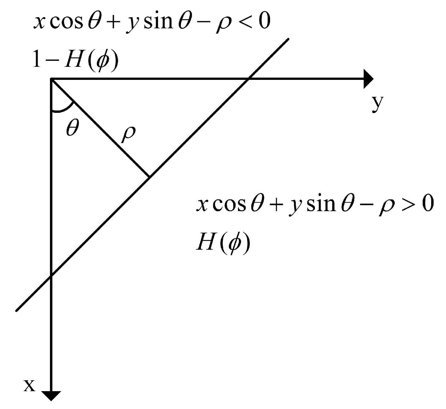
Since the function of a single line in the plane is
where
is the angle between the normal of the line and the positive direction of the x-axis, and
is the distance from the line to the origin.
Hence, as
Figure 6 shown, let the level-set function as:
Then, Equation (
10) can be solved by applying the gradient descent method. As the parameters
and
change with time
t during the evolution of the line, the evolution equation is obtained as [
31]:
By the gradient descent method, use
to iterative solution, where
a is a small constant, representing the learning rate;
represents the gradient of
. The
is the variable during the iteration and the
k is the iteration number.
After the iteration stops, segment the straight edge of image u.
3.3.3. Triangle Preserving Level-Set Model
Considering the triangular region as the intersection of three lines and detecting them one by one, the triangular target could be segmented.
Similar to the line model, the energy function of the Triangle Preserving level-set (TP) method is:
where the
represents a triangle area, which is shown in
Figure 7.
is written as:
When a line evolves, other lines are considered fixed, which means
and
are constants when solving for
. Therefore, set
and
, then reduce the problem from Equation (
15) to Equation (
10), and solve as Equation (
13). The other two lines are the same; then, the evolution formulae of Equation (
15) are:
where the
are the distances from the three lines forming the triangle to the origin,
are the angles of these three lines,
are the Heaviside function, and
are the Dirac function.
Similar to the line preserving level-set model, the gradient descent method is used to iteratively obtain the contour of the target. The algorithm flow is depicted in Algorithm 1.
| Algorithm 1: Triangle Preserving level-set. |
Input: image u, initial parameters of triangle 1: Initialization: learning rate a, positive fixed parameters , 2: while not converged do 3: calculate the by Equations ( 12) and ( 16) 4: calculate the average gray and of area and 1- area, respectively 5: calculate the gradient by Equation ( 17) with the fixed 6: calculate the gradient by Equation ( 17) with the fixed 7: calculate the gradient by Equation ( 17) with the fixed 8: calculate the by Equations ( 12) and ( 16) 9: update by gradient descent method 10: end while |
Note that there is another possible form of the
. The details can be found in
Appendix A.
The intersection points of the three lines are the three robust feature points. Assume that the lines
and
intersect at point
, then we have
and the solution is
The two other intersections are similar to this.
3.3.4. Process of Ship Target with TP
Before using the TP method for image segmentation, providing suitable initial values of can accelerate the iteration. Different from the previous section, three initial lines are estimated by three initial feature points in this section, further obtaining the initial values . Although these scatterers may be affected by speckle noise, stripes, and angle glint, they will be stably detected by the TP method.
In summary, the process of extracting feature points from a ship with the TP method can be achieved through the following steps:
Step 1: Calculate the centroid of the preprocessed image u.
Step 2: Extract two scatterers farthest from the centroid in opposite directions one by one, then connect them as a line to obtain the scattered point farthest from the line. Record the three points as the initial points.
Step 3: Use these three points as the intersection points of three lines to calculate the initial values for .
Step 4: Apply Algorithm 1 to obtain the stable triangle.
Step 5: Obtain three intersection points of the corresponding three lines belonging to the triangle, and output them together with the centroid for the next algorithm.
After performing the TP method on the ship images, four points are outputs, including three feature points and one centroid point.
3.4. Triangle-Points Affine Transform Reconstruction
In the previous section, we extracted three stable points corresponding to the ship’s bow, stern, and island. Besides the three points, the centroid point is also considered as a robust point with less impact from speckle noise, stripes, and ship attitude. Therefore, adding the fourth point, the centroid point, can further reduce the impact of noise and improve the robustness of the TATR algorithm. Based on the three geometric feature points and one centroid point—a total of four points—the affine transform could be used to reconstruct the ISAR image to a standard attitude, reducing the sensitivity of attitude. The process is referred to as the Triangle-Points Affine Transform Reconstruction (TP-TATR).
The coordinates of the four points are written as
where the
,
are the coordinates of the four points. The coordinates of the four points after reconstruction are defined as
,
i = 1, 2, ..., 4. The affine transform can be written as:
where
and
are coefficients of the affine transformation.
Since there are six coefficients of the affine transformation existing in the matrix
A, only six equations are needed to obtain the solution. However, there are eight equations due to four points, bringing the equation group into the overdetermination. Therefore, we utilized the generalized inverse of the matrix to obtain the squares solution, which is:
where the
is the estimated affine transformation matrix.
In summary, the steps of TATR include:
Step 1: Based on the ISAR image, rewrite the four pairs of matching points’ coordinates as a matrix, including the bow, stern, island and the centroid.
Step 2: Estimate the transform matrix
using Equation (
22).
Step 3: Warp the ISAR image using the transform matrix , and output the result for recognition.
By applying an affine transformation using the to the ISAR image, the reconstructed image is the output of the TATR algorithm.
3.5. Template Matching
For the training data, the templates belonging to different categories can be obtained by averaging the standard ISAR images obtained by the TP-TATR method. Since the ISAR images after TP-TATR are robust with attitude sensitivity, only a few samples (five samples in this paper) are needed to complete the training. For the test data, after the TP-TATR, the images are matched with templates using the Normalized Product correlation (NProd) method [
32]. The formula is:
where
and
are the
ith pixel of test data images and templates, respectively.
The P ranges from 0 to 1, where 1 indicates a perfect correlation and 0 means no correlation. The samples are classified into the category of the template with the highest P.
4. Results and Discussion
4.1. Simulated Data
The 3D ship models were utilized to acquire the ISAR images from computational electromagnetics software for recognition processing. The simulation parameters were: center frequency = 8.5 GHz, bandwidth B = 150 MHz, and pulse interval stepping angle 0.01 degrees. The elevation angle ranges from 0 to 35 degrees. There were 128 cross-range points and 1024 range points in each ISAR image.
We selected three types of ships for modeling, and their 3D models and ISAR images are shown in
Figure 8. Target 1 has 77 ISAR images, target 2 has 127 ISAR images, and target 3 also has 127 ISAR images, adding up to 331 ISAR images.
In
Figure 8a, the ship’s island is biased to one side and there is a cylindrical structure above the island, with most of the scatterers mainly concentrated on the left side and a stronger scatterer at the top in
Figure 8b. In
Figure 8c, the ship contains multiple vertical structures and the island is mainly concentrated in the center of the ship, which is reflected in
Figure 8d as more scattering points in the center position. In
Figure 8e, the ship has an island and two vertical structures but, in
Figure 8f, the ISAR image only shows the island in the center of the ship, and the scatterers’ intensity of the two vertical structures is weak. It is obvious that the part of the relatively unique geometric structures of the ships can be reflected in the ISAR images.
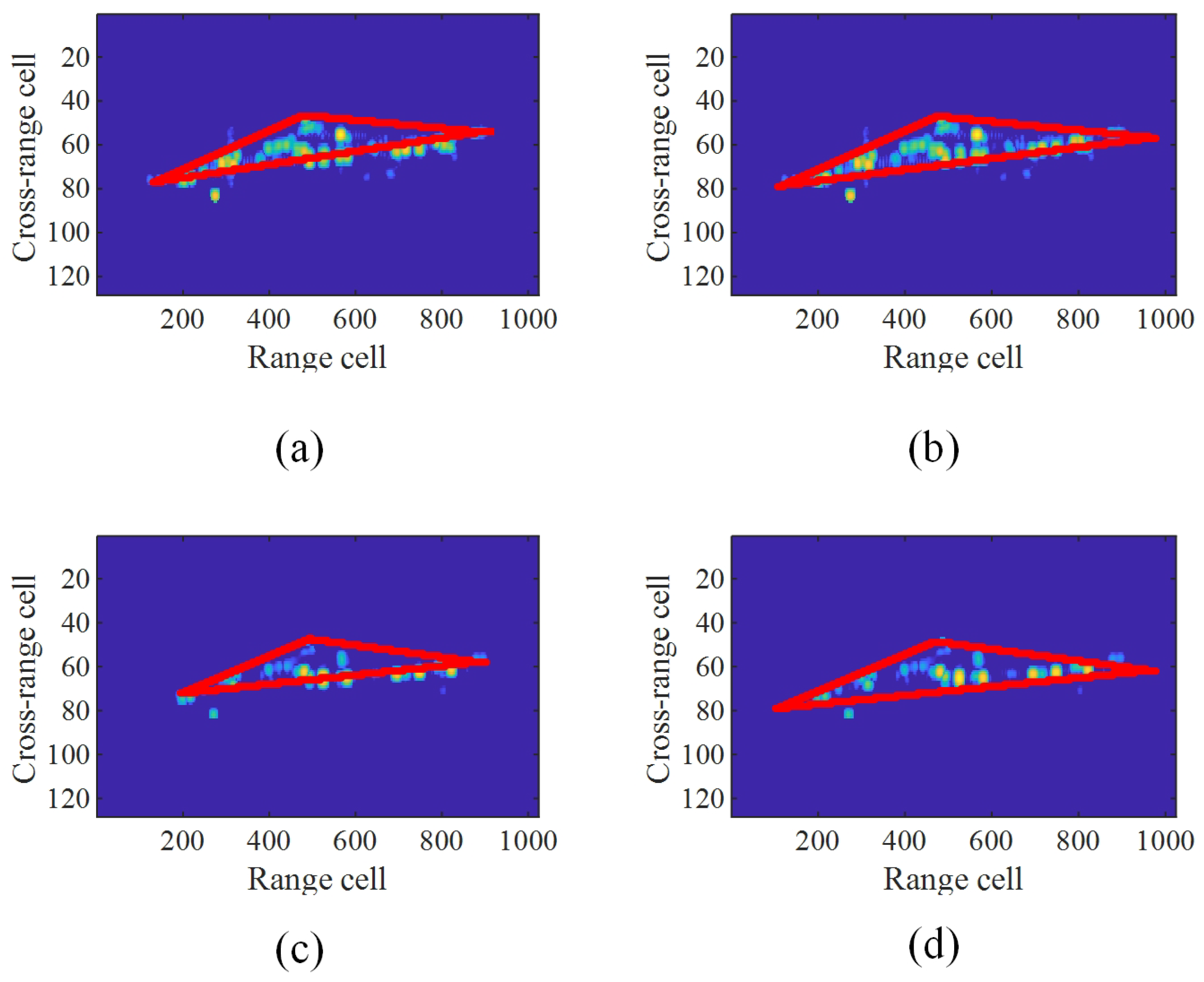
All the simulation ISAR images were preprocessed. Then the centroid was calculated, and three geometric structure feature points were extracted and are marked in
Figure 9. Compared
Figure 9a with
Figure 9c, some scatterers of structures disappear due to angle glint. Compared
Figure 9b with
Figure 9d, the location of the left feature point changes due to the scatterers weakened. The weakened scatterers interfere with the extraction of feature points. Therefore, we needed to extract robust feature points based on the TP method.
After the TP method, the results are shown in
Figure 10. Despite the differences between the input, the TP method can still stably segment the fitting triangle. We adopted the vertices of the triangle and the centroid point and applied the TATR algorithm.
The results of TATR are shown in
Figure 11. The targets are mostly corrected to horizontal postures, basically eliminating the elevation before TATR. From the result, we constructed a template for this type of target.
We used three ISAR images for each target type to construct templates, as shown in
Figure 12. The templates indicate that different images can be roughly overlapped after TATR reconstruction, and the ship’s position is relatively horizontal, demonstrating the stability of our algorithm.
To demonstrate the effectiveness of our algorithm, we designed comparative experiments with different algorithms. For fairness, each algorithm uses the same preprocessing and ISAR images to generate templates. The compared algorithms included the “only centroid” algorithm, which only aligns the centroid point to generate templates and matching, and the QATR [
34] algorithm, which uses the four vertices of the boundary rectangle and the centroid to reconstruct the ISAR images.
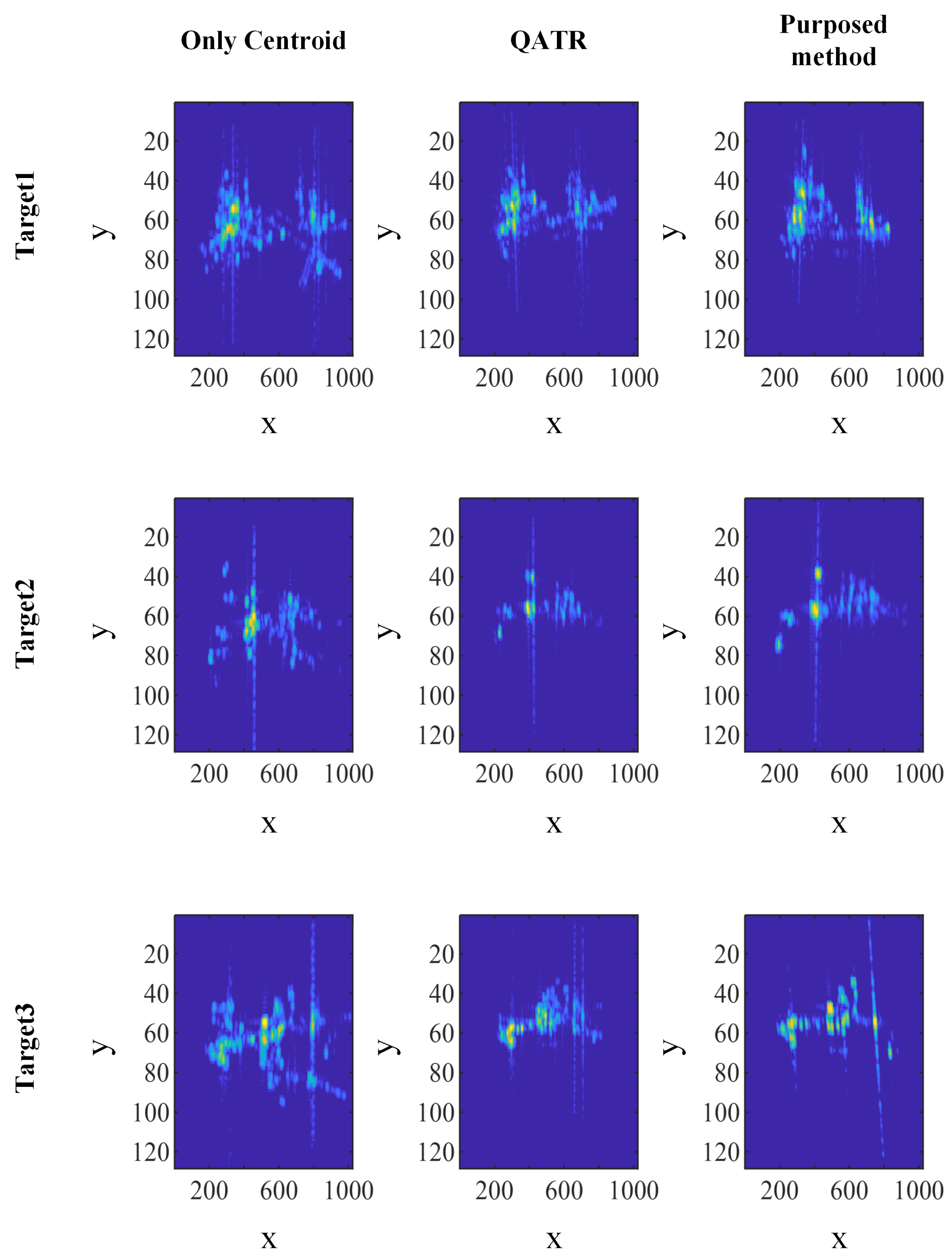
The templates generated by the above two algorithms and the proposed algorithm are shown in
Figure 13. The templates generated by the “only centroid” algorithm are difficult to use to recognize and identify useful information. Although the QATR algorithm performs better than the “only centroid” algorithm, the points may still be affected by the stripes caused by strong scattering points. As a result, sometimes the feature points deviate from the correct position, as shown in the template for target 1. Moreover, the angle glint may cause the template to appear “unfocused,” as shown in the template for target 3. Note that the template for target 3 appears to have two stripes, as the stripes caused by the same scatterers are not reconstructed to the same position.
In contrast, our proposed algorithm reconstructs ISAR images stably, and the obtained templates are advantageous for matching and recognition.
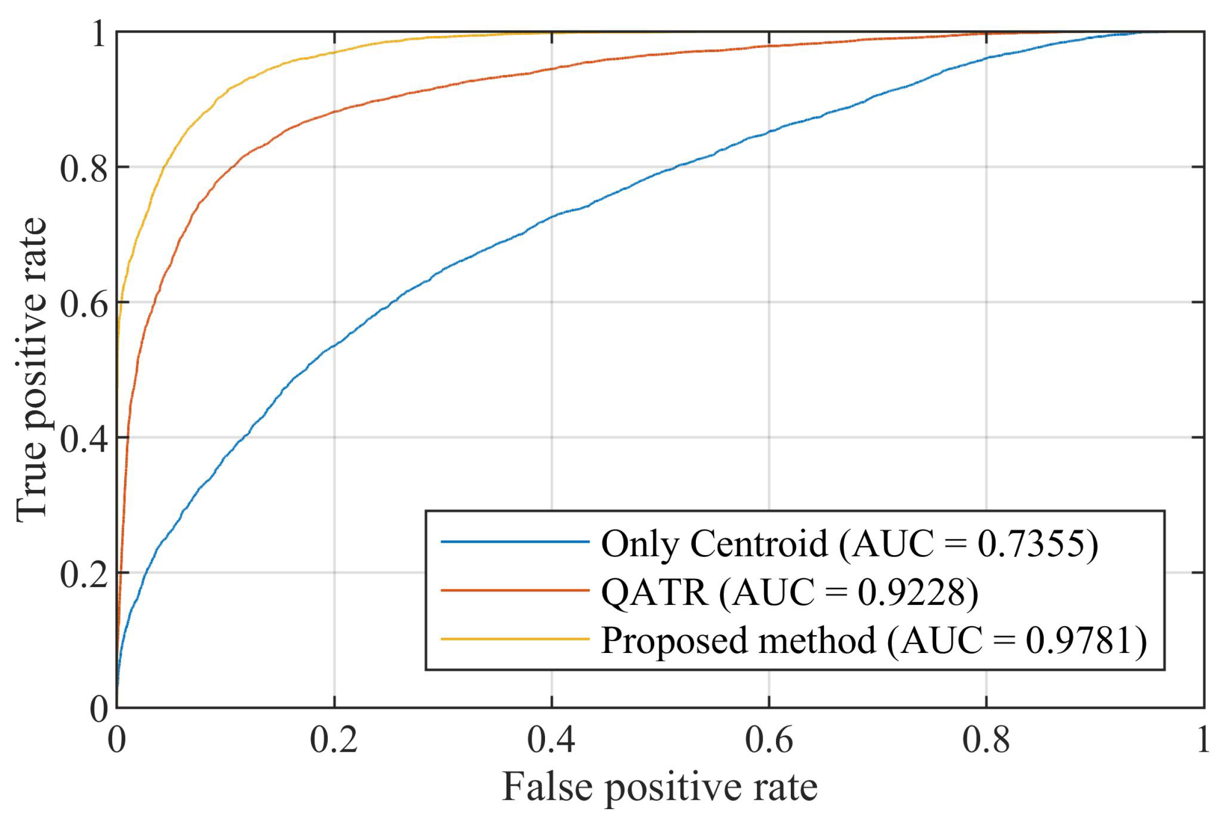
We used template matching on test data based on these templates. The Receiver Operating Characteristic (ROC) was drawn using the correlation of NProd, and the Area Under the Curve (AUC) was calculated [
37]. The result is shown in
Figure 14.
According to the figure, the “only centroid” method’s curve is the closest to the diagonal line, which means the worst recognition capability, and the AUC is lowest at 0.7355, accordingly. The curve of QATR is in the middle, meaning the recognition capability is better than “only centroid” but worse than our proposed method, and the AUC is in the middle—0.9228. The ROC curve demonstrates that our proposed method has the best recognition capability, as its curve is closest to the top-left, with the highest AUC at 0.9781. Each image was classified into the category of the template with the highest matching score. The accuracy of each algorithm is shown in
Table 1. This paper used Welch’s
t-test [
38] with statistical comparison. The
p-values of “only centroid” and QATR with the proposed method were calculated, and were
p < 0.001 and
p = 0.039 < 0.05, respectively. The results indicate that the accuracies of both methods are significantly different from that of the proposed method. It is clearly seen that the proposed method outperforms the others, further demonstrating the stability of our method.
4.2. Measured Data
The measured data were used to further verify the proposed method’s effectiveness.
The measured data were acquired using an X-band ISAR radar system with a bandwidth of 400 MHz. Each ISAR image was 128 points in the cross-range and 1024 points in the range direction. There were 66 ISAR images of a three-masted sailing ship, 42 ISAR images of a cargo ship, and 152 ISAR images of a transport ship, totaling 260 ISAR images.
Figure 15 shows the optical images of different targets and the corresponding ISAR image for each target. The ship in
Figure 15a has three masts, while in
Figure 15b it has three bright lines. The ship in
Figure 15c has four vertical structures and a ship island at the stern, which is also reflected in
Figure 15d. The ship in
Figure 15e has one vertical structure and a ship island, which is also obviously depicted in
Figure 15f.
Similar to the simulated data, the proposed method was validated on the measured data. Templates were obtained for the three types of targets using three, two, and five ISAR images, respectively, due to the disparity in the number of ISAR images for each target. The templates generated by our proposed method are shown in
Figure 16. The templates of measured data show that all the masts are almost overlapped at the same position, which are always vertical with the ship body in the image. The body of the ship is relatively horizontal. The stripes in the ISAR images of target 3 hardly disturb our algorithm. As a result, the stripes slope after TP-TATR. The templates demonstrate that different images can be roughly overlapped after TP-TATR reconstruction, indicating the stability of our algorithm with measured data. The templates obtained by the three algorithms are shown in
Figure 17, which shows the effectiveness of the proposed method.
For target 1, our method accurately aligns the slightly thinner structures, such as masts. For target 2, our algorithm can avoid the interference of stripes and accurately aligns the hull to the horizontal position. For target 3, the stripes converge near the scattering point near the bow of the ship, which indicates that the proposed algorithm can successfully align the scattering points near the bow under the interference of stripes, verifying the effectiveness and robustness of the proposed algorithm.
Similarly, by matching all ISAR images with the templates, the ROC was drawn using the correlation of NProd, and the AUC was calculated. The results are presented in
Figure 18.
Consistent with the results of simulated data, the “only centroid” method has the worst recognition capability, with its curve closest to the diagonal line and the lowest AUC at 0.7025. The QATR is in the middle, with both its curve and AUC at 0.9353. The best is our proposed method, with the curve closest to the top-left corner and the highest AUC at 0.9726.
The recognition results are shown in
Table 2. Welch’s
t-test was also used for hypothesis statistical testing. The results show that both the "only centroid” and the QATR algorithms have statistically significant differences with the algorithm proposed (with
p < 0.001 and
p = 0.005 < 0.05, respectively).
As this paper calculated the correlation between the test data and the templates to recognize ISAR images, the accuracy reflects the similarity of images after reconstruction. If the test data are similar to the templates, this means that the reconstruction process effectively reduces the influence of attitude sensitivity. Therefore, the recognition accuracy reflects the robustness of the reconstruction algorithm. The “only centroid” method only translates the ISAR images to the center, and the different images are uncorrelated, as influenced by the rotation. Therefore, the accuracy is the lowest. As with the proposed method, QATR also affines the image. However, the matching pairs of feature points are not accurate, which is influenced by the noise, strips, and angle glint, leading to rotated reconstructions that differ from the templates. The correlation between rotated images is lower, resulting in lower accuracy. The proposed method has the best robustness among these methods, and can adjust the images with different attitudes, resulting in the highest accuracy. which further proves the effectiveness of the proposed algorithm. In the future, we will focus on the effect of TP-TATR on more types of ships and different noise levels.


