An Improved Forest Height Model Using L-Band Single-Baseline Polarimetric InSAR Data for Various Forest Densities

Abstract

Forest density affects the inversion of forest height by influencing the penetration and attenuation of synthetic aperture radar (SAR) signals. Traditional forest height inversion methods often fail in low-density forest areas. Based on L-band single-baseline polarimetric SAR interferometry (PolInSAR) simulation data and the BioSAR 2008 data, we proposed a forest height optimization model at the stand scale suitable for various forest densities. This optimization model took into account shortcomings of the three-stage inversion method by employing height errors to represent the mean penetration depth and SINC inversion method. The relationships between forest density and extinction coefficient, penetration depth, phase, and magnitude were also discussed. In the simulated data, the inversion height established by the optimization method was 17.35 m, while the RMSE value was 3.01 m when the forest density was 100 stems/ha. This addressed the drawbacks of the conventional techniques including failing at low forest density. In the real data, the maximum RMSE of the optimization method was 2.17 m as the stand density increased from 628.66 stems/ha to 1330.54 stems/ha, showing the effectiveness and robustness of the optimization model in overcoming the influence of stand density on the inversion process in realistic scenarios. This study overcame the stand density restriction on L-band single baseline PolInSAR data for forest height estimation and offered a reference for algorithm selection and optimization. The technique is expected to be extended from the stand scale to a larger area for forest ecosystem monitoring and management.

1. Introduction

Forests are significant contributors to the global carbon cycle. Forest height is a crucial input variable for building biomass models and assessing the condition of forest resources. Traditional forest surveys obtain forest height through field measurements. This approach can only obtain small-scale data on a point-by-point basis, while at the same time consuming both human and material resources. It is challenging to obtain forest data on a large scale, but remote sensing is best suited to address this challenge. The commonly used remote sensing techniques include optical remote sensing, Lidar, synthetic aperture radar (SAR) methods, and so on. Optical remote sensing can obtain information on forest biomass, species, and biochemical properties. However, optical remote sensing is not penetrating and is susceptible to cloud cover and weather, thus limiting its use [1]. LiDAR can provide high-precision information about the vertical structure of the forest, but it is also affected by weather, such as clouds, fog, and rain [2]. Additionally, the observation area is small, and the acquisition cost is high [3]. SAR signals have strong penetration and are not affected by the weather. In recent years, SAR has developed the capability to monitor the vertical and horizontal structure of features continuously and has excellent potential to estimate forest height and above-ground biomass (AGB) on a global scale [4,5].

Polarimetric SAR interferometry (PolInSAR) is one of the SAR techniques that has received much attention in recent years. PolInSAR uses the interferometric phase to observe the vertical structure of the forests. The technique uses the sensitivity of polarization to the shape, dielectric properties, texture, and orientation of the scatterers to identify different scattering mechanisms of the target [6]. Based on PolInSAR inversion models, several researchers have effectively achieved the inversion of forest height and AGB [7,8]. The DEM difference method [9], RVoG ground phase method [10], SINC inversion method [11], phase and coherence inversion method [12], and three-stage inversion method [13] are the popular PolInSAR inversion models. Among these, the three-stage inversion method based on the random volume over ground (RVoG) model minimizes the complexity of the inversion model, expanding the application of the RVoG method.

The RVoG model uses a mathematical model to connect the forest parameters to the SAR system parameters. Most current RVoG models and their improvement methods are mainly concerned with the optimization of model parameters. The key points and difficulties of the vegetation scattering model are how to estimate the ground phase accurately and effectively separate the ground scattering contribution from the canopy scattering contribution. Many researchers enhance the separation of two-phase centers using the singular value decomposition (SVD) [14] and phase diversity (PD) coherence optimization method [15] to precisely determine the ground phase.

On the other hand, some studies have focused on the effect of scenes on the vegetation scattering model. Since the RVoG model initially focused on airborne data, it did not consider the impact of terrain and temporal decorrelation [10,16]. Temporal decorrelation and terrain distortion in real scenarios lead to the limitations of traditional models in practical applications [17,18,19]. Lu et al. suggested the sloped random volume over ground (S-RVoG) model, which accounts for the influence of terrain slope on PolInSAR data inversion. S-RVoG rectifies the forest parameters by including the range slope in the RVoG model and demonstrating the validity using L-band simulation data [20]. XIE et al. showed that the S-RVoG model corrected terrain slope and improved forest height inversion accuracy using P-band dual-baseline PolInSAR data [21]. Cloude et al. proposed the random volume over ground with volume temporal decorrelation (RVoG+VTD) model. The RVoG+VTD model only considers the effect of temporal decorrelation on the coherence amplitude [22]. Later, various researchers presented the temporal decorrelation random volume over ground with volume (TD-RVoG) model, the random motion over ground (RMOG) model, and the semi-empirical forest height inversion approach to transform temporal decorrelation into a complex form [23,24,25,26].

However, the forest density also degrades the inversion results, making the ability of the vegetation scattering model less effective. Forest density affects forest characteristics (extinction coefficient, ground phase, forest height) and SAR system parameters (amplitude, phase) by influencing the penetration and attenuation of the SAR signal. Thick forests diminish the degree of complex coherence separation, resulting in erroneous estimation of the ground phase [13]. Xie et al. discovered that high forest density had a substantial canopy scattering contribution, resulting in an underestimating of the inversion findings after adjusting terrain slope [27]. Meanwhile, Garestier et al. employed X-band data to invert sparse coniferous forests. Low forest density causes extensive canopy gaps, allowing short wavelength PolInSAR data to penetrate the canopy and result in forest height inversion [28]. Wang et al. used simulated and P-band BioSAR 2008 data to show that the traditional three-stage inversion method failed to invert in sparsely vegetated areas. Noteworthy, forest density is positively correlated with ground phase estimation accuracy and negatively correlated with ground-to-volume scattering ratio [29]. Most current vegetation scattering model studies focuses on the qualitative relationship between forest density and model parameters. In this paper, we present an improved method applicable to various forest densities based on a study of the influence of forest density on SAR system parameters and forest characteristics.

In this study, we first analyze the forest height inversion results of five commonly utilized PolInSAR inversion models using simulated data of different forest densities. By comprehensively analyzing the relationships and regulations of forest density and forest parameters, we propose the coherence magnitude and three-stage hybrid theoretical method applicable to various forest densities. The model uses the forest height error to represent the average penetration depth of various forest densities. The adjustment coefficients are selected iteratively according to different forest stands’ characteristics and penetration depth. Finally, the SINC inversion method, three-stage inversion method, and adjustment coefficients constitute the model. Comparing the inversion results of the improved model with those of the traditional model shows that the hybrid iterative theoretical process achieves single-baseline PolInSAR forest height inversion for different forest densities. In particular, it overcomes the shortcomings of conventional approaches to inversion failure at low forest density. The improved model was validated using actual SAR data. Furthermore, a slope correction algorithm and PD coherence optimization algorithm were introduced to the hybrid iterative theoretical method to form the coherence magnitude and three-stage hybrid iterative application model (hybrid iterative application model). The optimization model achieves high accuracy inversion in real scenarios with different forest densities and enables a reference for future research.

2. Datasets and Pre-Processing

2.1. PolSARproSim Simulated Datasets

This study aims to investigate the effects of different forest densities on the widely employed PolInSAR inversion methods and the effectiveness of the improved model under various forest densities, which requires controlling the same forest height and reducing the impact of temporal decoherence. The experimental conditions are more stringent, and obtaining ideal airborne SAR data is more complicated. The ESA’s PolSARpro software allows the user to flexibly set the platform configuration, forest/ground surface configuration, and other parameters for data simulation to build the ideal experimental conditions [30,31].

To study the effect of forest density on the tree height inversion technique, PolSARproSim built a simulated airborne L-band (central frequency 1.3 GHz) PolInSAR dataset, which contains nine groups of forest densities ranging from 100 stems/ha to 900 stems/ha. The other parameters in the simulated dataset are similar and kept fixed, as shown in

Table 1. ESA’s PolSARproSim module simulated nine groups of stand-specific parameters. Coniferous forest densities ranged from 100 stems/ha to 900 stems/ha. The reference heights are all 18 m, the azimuth and range slope are all 0, and the ground roughness and soil wetness are 0. Terrain, shrub layer, and temporal decoherence do not influence the echo signal or inversion technique.

Platform Configuration	Parameter	Forest/Ground Surface Configuration	Parameter
Platform Altitude	3000 m	Tree Species	Pine
Horizontal/Vertical Baseline	10 m,1 m	Surface Properties/Ground Moisture Content	0,0
Incidence Angle	45°	Azimuth/Range Ground Slope	0
Centre Frequency	1.3 GHZ	Tree Height	18 m

. The forest density indicator in the data set is the tree number per hectare (stems/ha), and the forest density of 100 stems/ha, 200 stems/ha, 300 stems/ha, 400 stems/ha, 500 stems/ha, 600 stems/ha, 700 stems/ha, 800 stems/ha, and 900 stems/ha coniferous forest, the slope in both azimuth and range directions is 0. The ground roughness and soil moisture are also 0. Terrain, shrub layer, and temporal decoherence do not influence the echo signal or inversion technique. Figure 1 illustrates scenario images for nine groups of simulated datasets, and Figure 2 displays Pauli-basis images for nine groups of simulated datasets.

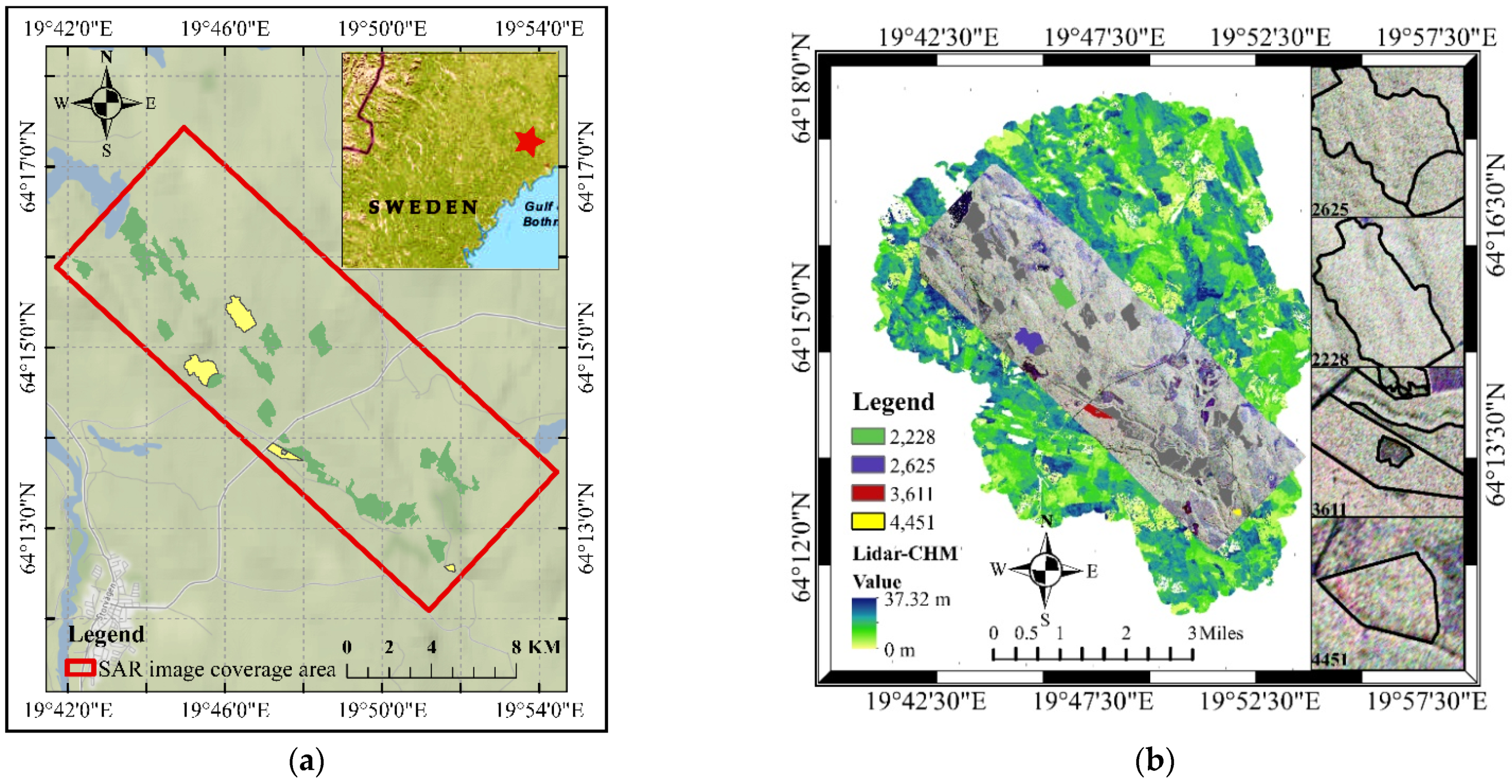
2.2. The BioSAR 2008 Datasets

Airborne L-band PolInSAR data from the Krycklan catchment in northern Sweden, taken during ESA’s BioSAR 2008 experiment, were used for model validation in this study. The BioSAR 2008 campaign acquired high-latitude boreal forest data with terrain impacts to investigate the BIOMASS mission’s potential for estimating biomass in boreal forests. The test site (64°14′N, 19°46′E) is in Vindeln municipality, situated in Sweden (Figure 3a), with elevation changes from 100 m to 300 m and mixed coniferous forest as the dominating forest type. The dataset is available on the ESA by application and includes airborne SAR data, field inventory data such as Lidar data, DEM data, and 31 forest stands.

In 2008, 31 forest stands were field-surveyed, and ArcGIS software was used to generate vector contour polygons (yellow polygons in Figure 3a). The stand-level tree height, volume, and biomass were estimated and corrected using measured data and static functions. The guidebook explains the specific prediction technique and field survey process [32]. Because this research investigates the influence of forest density on the inversion of PolInSAR data, we consider tree species composition, stand mean height, and forest density as indicators to select among 31 forest stands. This was also to ensure that the experimental conditions of the realistic and simulated datasets were comparable. In this study, the four pure coniferous stands (stand numbers 4451, 2625, 3611, and 2228) with forest density of 628.660 stems/ha, 840.340 stems/ha, 1149.100 stems/ha, and 1330.540 stems/ha, respectively, and the average tree height measured in the field (nearly 18 m) were nearly similar to a real-world scenario for algorithm validation. The gap in forest density between neighboring forest stands is 200 stems/ha. The range of forest density was vast, with a difference of 700 stems/ha between the lowest and the highest forest density, which was consistent with the experimental goal of this work.

The two images of L-band PolInSAR data collected on 15 October 2008, were taken as real-world data for testing the inversion model in this work. The SceneIDs were 08BioSAR0201 × 1 and 08BioSAR0205 × 1, respectively, as shown in

Table 2. BioSAR 2008 L-band PolInSAR data specific parameter information. The sceneIDs of master and slave images are 08BioSAR0201 × 1 and 08BioSAR0205 × 1, respectively.

Scene ID	Baseline (m)	Kz	Band	Polarization
08BioSAR0201	Master 0 m	Master	L	Quad
08BioSAR0205	Slave 12 m	0.046–0.370	L	Quad

. The pre-processing of the master and slave images mainly includes coregistration, removing the flat-earth phase, multilooking, 7’7 LEE refined speckle filtering [33], and using 50 m × 50 m DEM for geocoding [34]. Figure 3b shows the SAR image and LiDAR image of WGS84 UTM Zone 34N on the left side and the shapes of the four forest stands on the right side.

3. Methodology

This study uses five common inversion methods in the simulated dataset to investigate the effect of forest density on the PolInSAR inversion process. According to the features of the three-phase inversion technique and SINC inversion method, a coherence magnitude and three-stage hybrid iterative inversion method are suited for various forest densities. The terrain-corrected incidence angle and vertical wavenumber were introduced into the coherence amplitude and three-phase hybrid iterative inversion model to reduce terrain’s impact on the inversion model. The model without terrain correction is called the coherence magnitude and three-stage hybrid iterative inversion theory method. The coherence magnitude and three-stage hybrid iterative inversion application model is the model with terrain correction. Figure 4 depicts the flowchart of the study.

3.1. Typical Models for the PolInSAR Technique of Forest Height Inversion

The DEM Difference Model determines the forest height $h_v$ by comparing the phase differences and vertical wavenumbers $k_z$ of the two polarization modes representing the canopy and ground scattering centers. The key to this technique is determining the two polarization states representing forest canopy scattering and ground scattering, as shown in Equation (1) [6].

$$h_v=\frac{\mathit{arg}({\gamma }_{w_v})-\mathit{arg}({\gamma }_{w_g})}{k_z}$$

(1)

$$k_z=\frac{\mathit{4}\pi \Delta \theta }{\lambda \mathit{sin}\theta }\approx \frac{\mathit{4}\pi B_{\perp }}{\lambda R\mathit{sin}\theta }$$

(2)

where $w_g$ and ${\gamma }_{w_g}$ mean the ground scattering mechanism and the ground scattering complex coherence, respectively. ${\gamma }_{w_v}$ is the volume scattering complex coherence and $w_v$ is the forest canopy scattering mechanism, respectively. $\theta$ is the radar angle of incidence; $\lambda$ represents the radar wavelength; $R$ represents the radar slant range, and $B_{\perp }$ represents the perpendicular baseline. Although this approach is theoretically simple, the results often underestimate 1/3 of the actual tree height [35].

The Three-Stage Inversion Method represents complex coherence coefficients of different polarizations that are linearly distributed in the complex unit circle. The RVoG model is decomposed into a linear structure. The quantitative inversion process of vegetation parameters is divided into three stages (Equation (3)) [10,28].

Using the least squares algorithm to fit a straight line in the complex plane;

Estimating the actual ground phase point based on the intersection of the fitted line with the complex unit circle;

Inverting the tree height and extinction coefficient using a height-extinction coefficient two-dimensional look-up table (LUT).

$$\begin{array}{ll}\gamma \left(w\right)& =e^{j{\varphi }_{\mathit{0}}}\frac{{\gamma }_v+m\left(w\right)}{\mathit{1}+m\left(w\right)}\\ & =e^{j{\varphi }_{\mathit{0}}}\left[{\gamma }_v+\frac{m\left(w\right)}{\mathit{1}+m\left(w\right)}\left(\mathit{1}-{\gamma }_v\right)\right],L_w=\frac{m\left(w\right)}{\mathit{1}+m\left(w\right)}\\ & =e^{j{\varphi }_{\mathit{0}}}\left[{\gamma }_v+L_w\left(\mathit{1}-{\gamma }_v\right)\right]\end{array}$$

(3)

$$\begin{array}{ll}{\gamma }_v& =\frac{{\displaystyle {\int }_{\mathit{0}}^{h_v}f\left(z\right)e^{j{k}_{z}z}dz}}{{\displaystyle {\int }_{\mathit{0}}^{h_v}f\left(z\right)dz}}=\frac{\mathit{2}\sigma }{\mathit{cos}\left(e^{\mathit{2}\sigma h_v/\mathit{cos}\theta }-\mathit{1}\right)}{\displaystyle {\int }_{\mathit{0}}^{h_v}{e}^{j{k}_{z}z}{e}^{\frac{\mathit{2}\sigma z}{\mathit{cos}\theta }}dz}\\ & =\frac{\mathit{2}\sigma }{\mathit{2}\sigma +j{k}_z\mathit{cos}\theta }\cdot \frac{\mathit{exp}\left(\mathit{2}\sigma h_v/\mathit{cos}\theta +j{k}_z{h}_v\right)-\mathit{1}}{\mathit{exp}\left(\mathit{2}\sigma h_v/\mathit{cos}\theta \right)-\mathit{1}}\end{array}$$

(4)

where ${\gamma }_v$ is the pure complex coherence of the forest canopy, and $L_w$ is the ground scattering ratio for a given polarization state $w$. $m\left(w\right)$ is the ground-to-volume scattering ratio. $\sigma$ is the extinction coefficient, representing the energy loss of electromagnetic waves through the medium. $f\left(z\right)$ is the vegetation vertical structure function, which is usually simplified to an exponential function in the RVoG model.

The RVoG Ground Phase Method (Equation (5)) is an improved model of the DEM difference method. The RVoG model is used to compute $L_{w_g}$, which is then introduced in the DEM difference method to estimate forest height (Equations (6) and (7)). The approach inverses forest height is better than the DEM difference method, but it still underestimates forest height [7].

$$h_v=\frac{\mathit{arg}({\gamma }_{w_v})-{\varphi }_{\mathit{0}}}{k_z}$$

(5)

$$\begin{array}{ll}{\varphi }_{\mathit{0}}& =\mathit{arg}\left[{\gamma }_{w_g}-{\gamma }_{w_v}\left(\mathit{1}-L_{w_g}\right)\right]\\ & \Rightarrow \{\begin{array}{c}{\gamma }_{w_v}=e^{j{\varphi }_{\mathit{0}}}{\gamma }_v\\ {\gamma }_{w_g}=e^{j{\varphi }_{\mathit{0}}}\left[{\gamma }_v+\frac{m\left(w_g\right)}{\mathit{1}+m\left(w_g\right)}\left(\mathit{1}-{\gamma }_v\right)\right]\end{array},L_{w_g}=\frac{m\left(w_g\right)}{\mathit{1}+m\left(w_g\right)},\mathit{0}\le L_{w_g}\le \mathit{1}\\ & \Rightarrow {\gamma }_{w_g}={\gamma }_{w_v}+L_{w_g}\cdot e^{j{\varphi }_{\mathit{0}}}-L_{w_g}\cdot {\gamma }_{w_v}\\ & \Rightarrow e^{j{\varphi }_{\mathit{0}}}=\frac{{\gamma }_{w_g}-{\gamma }_{w_v}\left(\mathit{1}-L_{w_g}\right)}{L_{w_g}}\end{array}$$

(6)

$$\begin{array}{l}A{L}^{\mathit{2}}{}_{w_g}+B{L}_{w_g}+C=\mathit{0}\Rightarrow L_{w_g}=\frac{-B-\sqrt{B^{\mathit{2}}-\mathit{4}AC}}{\mathit{2}A}\\ A={\left|{\gamma }_{w_v}\right|}^{\mathit{2}}-\mathit{1},B=\mathit{2}Re\left(\left({\gamma }_{w_g}-{\gamma }_{w_v}\right){\gamma }^{*}{}_{w_v}\right),C={\left|{\gamma }_{w_g}-{\gamma }_{w_v}\right|}^{\mathit{2}}\end{array}$$

(7)

The SINC Inversion Method assumes a zero extinction coefficient, ignores ground scattering, and inverts forest height directly using coherence magnitude representing canopy scattering coherence. So, the SINC inversion method is also known as the coherence magnitude inversion method [7,8]. The RVoG model (3) is simplified to a random volume (RV) scattering model (Equation (4)). The forest height $h_v$ and volume scattering complex coherence ${\gamma }_{w_v}$ show a SINC function connection under this assumption, as seen in Equation (8). This approach generally overestimates tree height.

$$\begin{array}{ll}{\gamma }_{w_v}& =\underset{\sigma \to \mathit{0}}{\mathit{lim}}\left[\frac{{\displaystyle {\int }_{\mathit{0}}^{h_v}f\left(z\right)e^{j{k}_{z}z}dz}}{{\displaystyle {\int }_{\mathit{0}}^{h_v}f\left(z\right)dz}}\right]=e^{\frac{\mathit{1}}{\mathit{2}}j{k}_z{h}_v}\frac{\mathit{sin}\left(\frac{\mathit{1}}{\mathit{2}}{k}_z{h}_v\right)}{\frac{\mathit{1}}{\mathit{2}}{k}_z{h}_v}\\ & \Rightarrow h_v=\frac{\mathit{2}\cdot \mathit{sin}{c}^{-\mathit{1}}\left(\left|{\gamma }_{w_v}\right|\right)}{k_z}\end{array}$$

(8)

The Phase and Coherence Inversion Method combines the RVoG ground phase method (first term of Equation (5)), which underestimates tree height, and the SINC inversion method (second term of Equation (8)), which overestimates tree height. The model has a more robust structure and low computational complexity. Some researchers compared the phase and coherence inversion method to other methods and discovered that the phase and coherence inversion method has the best inversion property and is easier to use. Additionally, it is vulnerable to the accuracy of the RVoG ground phase method [9]. The correction factor $\epsilon$ in this investigation sets to 0.4 due to the absence of a priori knowledge.

$$h_v=\frac{\mathit{arg}({\gamma }_{w_v})-{\varphi }_{\mathit{0}}}{k_z}+\epsilon \cdot \frac{2\mathit{sin}{c}^{-1}\left(\left|{\gamma }_{w_v}\right|\right)}{k_z}$$

(9)

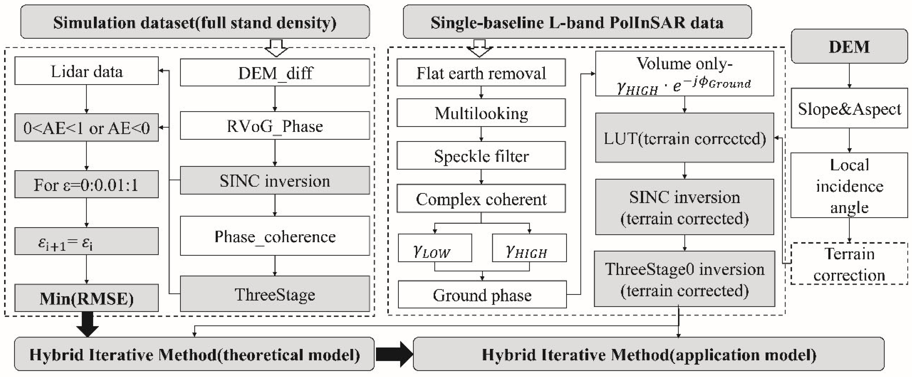
3.2. Coherence Amplitude and Three-Stage Hybrid Iterative Model

3.2.1. Coherence Amplitude and Three-Stage Hybrid Iterative Theoretical Model

The classic SINC Inversion Method often overestimates the height of the forest because it assumes that the ground scattering contribution is zero and that the volume scattering contribution dominates the interferometric coherence. The three-stage inversion method has greater accuracy than the SINC inversion method, DEM difference method, and RVoG ground phase method. It simplifies the complexity of the height inversion model. However, several studies have shown that the results of the three-stage inversion method remain to underestimate the height of the forest. The three-stage inversion method’s results typically underestimate [36,37] because the algorithm assumes that the ground-to-volume scattering ratio of HV polarization is zero. Additionally, all polarizations in real scenarios contain some ground scattering contribution.

Additionally, this inversion approach takes more time. The LUT steps can be used to produce more precise results for forest height and extinction coefficients, but this will result in a massive rise in the model’s inversion time because the LUT must invert each pixel. Another disadvantage is that the images’ uniformity impacts the traditional three-stage inversion method. Forest density influences the attenuation of SAR signals in the canopy layer, which causes errors in the inversion. The RVoG two-layer scattering model assumes that the volume layer is a random medium with uniform density (see, for example, Figure 5). Still, low forest density is no longer considered a homogeneous medium, and applying the RVoG model under such inhomogeneous vegetation conditions affects the accuracy of the inversion results [26].

This study improves the forest height inversion model by combining the three-stage inversion method and the SINC inversion method based on the model structure of the phase and coherence inversion approach. The traditional three-stage inversion method is not suitable for the inversion of sparse vegetation conditions and underestimates forest height. According to previous research, both the RVoG ground phase method and the three-stage inversion method underestimate forest height. The three-stage inversion method is used in place of the RVoG ground phase method in the traditional phase and coherence inversion method, where $ThreeStage$ represents the three-stage inversion method. The three-stage inversion method’s relative error $AE$ and the magnitude term ($\frac{2\mathit{sin}{c}^{-1}\left(\left|{\gamma }_{w_v}\right|\right)}{k_z}$) compensate for $ThreeStage$ to solve the problem of forest height underestimation under sparse vegetation conditions, which is associated with the three-stage inversion method (Equation (10)). When the pixel’s result is overestimated, $AE<0$; and when the pixel’s effect is underestimated, $AE>0$. The average tree height ($realvalue$) represents the average level in a forest stand and it is used in inversion to decrease the complexity of collecting real-world data. In this paper, we used average tree height to obtain penetration depth. Section 5.3 discusses the relationship between penetration depth and forest density.

$$\begin{gathered} AE<0 \\ {h}_v=ThreeStage+AE\cdot {\epsilon }_i\cdot \frac{2\mathit{sin}{c}^{-1}\left(\left|{\gamma }_{w_v}\right|\right)}{k_z} \end{gathered}$$

(10)

$$AE=(realvalue-ThreeStage)/realvalue$$

(11)

The traditional phase and coherence inversion approach needs the model adjustment coefficients to be generated based on a priori information. The same weighting factor $\epsilon$ is employed for each pixel in the inversion process to correct the magnitude term for the phase term. Although using a single $\epsilon$ for the entire image simplifies the inversion process, it has obvious disadvantages when the SAR image contains forest conditions with varying forest density or forest types. This study uses the adjustment coefficients ${\epsilon }_i$ to control the minimization of inversion error RMSE by instructing each pixel to select the adjustment coefficient with the minimum forest height error $\epsilon =\mathit{arg}\left(RMS{E}_{\min }\right)$ in i iterations. The new weighting term $AE\cdot {\epsilon }_i$ strengthens the entire model’s structure. It overcomes the drawbacks of the three-stage inversion method, which is better suited for inversion under whole-forest density situations, but fails under sparse forest conditions. The following summarizes the inversion procedure of the coherence amplitude and three-stage hybrid iterative approaches.

Linear least-squares fitting of all complex coherence coefficients in the complex unit circle. This stage follows the traditional three-stage inversion method.

Obtaining of the actual ground phase. The fitted line and the complex unit circle intersect at (${\varphi }_1,{\varphi }_2$). The HV channel usually represents the volume scattering complex coherence and HH-VV channel represents the ground scattering complex. The intersection farthest from HV represents the actual ground phase ${\varphi }_{ground}$;

$${\varphi }_{ground}=\{\begin{array}{cc}{\varphi }_1\Leftarrow & \left|e^{i{\varphi }_1}-{\gamma }_{HV}\right|>\left|e^{i{\varphi }_1}-{\gamma }_{HH-VV}\right|\\ {\varphi }_2\Leftarrow & else\end{array}$$

(12)

Calculation of forest height. The iteration range of forest height and extinction coefficient are first set, then the pure volume scattering complex coherence $LUT\left(h_v,\sigma \right)$ is constructed using Equation (13). The distance between the volume scattering complex coherence and the LUT whose ground phase has been removed is calculated. The smallest distance calculated on the LUT is the most appropriate forest height and extinction coefficient;

$$h_{ThreeStage}=\underset{\left(height,\sigma \right)}{\mathit{arg}\min }\left\{\left|{\gamma }_{HV}{e}^{-i{\varphi }_{ground}}-LUT\left(h_v,\sigma \right)\right|\right\}$$

(13)

Equation (8) generates the SINC inversion method’s findings with an extinction coefficient of 0;

Determining the relative error of the height $AE$ of each image pixel from the tree height and the three-stage Inversion method’s forest height, and applying a weighting coefficient ${\epsilon }_i\left(0\le {\epsilon }_i\le 1\right)$ to each image pixel. Equation (10) includes the weighting factor $AE\cdot {\epsilon }_i$. The image pixel is iterated by image element based on the minimized RMSE, and the appropriate $\epsilon =\mathit{arg}\left(RMS{E}_{\min }\right)$ is determined.

3.2.2. Coherence Magnitude and Three-Stage Hybrid Iterative Application Model

The coherence magnitude and three-stage hybrid iterative theoretical model (Equation (10)) apply to ideal conditions, i.e., flat areas with no terrain effects or temporal decoherence, which is compatible with the traditional RVoG model. A large number of studies, however, have demonstrated that the conventional RVoG model is sensitive to terrain effects: the higher the slope of the terrain, the higher the inversion error; the higher the forest height, the higher the inversion error [17,18,24]. As a result, this work employs a widely used slope correction approach to improve the theoretical model [15]. In non-flat locations, vegetation is distributed along the surface’s slope, and the traditional RVoG model assumes that the vegetation is in a flat area. Because of the presence of the terrain slope $\alpha$, the local coordinate system of the ground surface patch (P) is corrected from $yoz$ to $y^{\prime }{o}^{\prime }{z}^{\prime }$, as illustrated in Figure 6. When the terrain slope facing the radar sensor is positive (Figure 6a), the corrected local incidence angle ${\theta }_0$ is smaller than the original radar incidence angle $\theta$, and the vertical wavenumber increases. When the terrain slope facing the radar sensor is negative (Figure 6b), the local incidence angle ${\theta }_0$ is larger than the original radar incidence angle $\theta$, and the vertical wavenumber decreases. The terrain slope affects the volume complex coherence by influencing the pixel’s radiometric brightness and vertical wavenumber [15]. The radar incidence angle may be corrected using the terrain slope to produce the local incidence angle ${\theta }_0$, while the original $k_z$ uses the local incidence angle ${\theta }_0$ to correct it.

$${\theta }_0=\theta -\alpha$$

(14)

$$k_{z\mathit{0}}=\frac{\mathit{4}\pi B_{\perp }}{\lambda R\mathit{sin}{\theta }_{\mathit{0}}}$$

(15)

The RVoG model’s volume coherence is then corrected using $k_{z\mathit{0}}$:

$${\gamma }_v=\frac{\mathit{2}\sigma }{\mathit{2}\sigma +j{k}_{z\mathit{0}}\mathit{cos}{\theta }_{\mathit{0}}}\cdot \frac{\mathit{exp}\left(\left(\mathit{2}\sigma h_v/\mathit{cos}{\theta }_{\mathit{0}}+j{k}_{z\mathit{0}}{h}_v\right)\cdot \mathit{cos}\alpha \right)-\mathit{1}}{\mathit{exp}\left(\mathit{2}\sigma h_v/\mathit{cos}{\theta }_{\mathit{0}}\cdot \mathit{cos}\alpha \right)-\mathit{1}}$$

(16)

The forest heights acquired by inversion were all along the $y^{\prime }{o}^{\prime }{z}^{\prime }$ coordinate system, and the terrain-corrected forest heights were $h_{v0}$ as illustrated in in Figure 6. Thus, it is essential to project $h_{v0}$ to the $yoz$ coordinate system to obtain the forest heights $h_{ThreeStage}$ according to Equation (17) [17,38]. Meanwhile, some studies have shown that the range component of terrain slope is the dominant effect, and the azimuth slope is a minor one. Therefore, this study only considers the range slope correction. Figure 7 shows the slope and DEM of the four forest stands.

$$h_{ThreeStage0}=\frac{h_{v0}}{\mathit{cos}\left|\alpha \right|}$$

(17)

The hybrid iterative algorithm is modified at this point to use the terrain-corrected three-stage inversion method $ThreeStage0$ to replace the first term of the theoretical model. The vertical wavenumber $k_{z0}$ was corrected to reduce the impact of terrain on the SINC inversion method (Equation (18)).

$$h_v=ThreeStage0+AE\cdot {\epsilon }_i\cdot \frac{2\cdot \mathit{sin}{c}^{-1}\left(\left|{\gamma }_{w_v}\right|\right)}{k_{z0}}$$

(18)

The traditional SINC inversion method uses the coherence amplitude of a particular polarization channel, such as HV or $P{D}_{HIGH}$. It assumes that its ground scattering contribution is zero to invert the forest height. In reality, all polarization channels have ground-scattering components. The extra ground scattering coherence amplitude causes overestimation of the SINC Inversion Method. The second stage of the three-stage inversion method obtained the actual ground phase, which was removed from the assumed pure volume complex coherence. At this stage, the pure-volume complex coherence is the most suitable input variable for the SINC inversion method. As a result, we employ the pure volume complex coherence to replace the second term of Equation (18), obtaining the application model of the coherence magnitude and the three-phase hybrid iterative approach (Equation (19)).

$$h_v=ThreeStage0+AE\cdot {\epsilon }_i\cdot \frac{2\cdot \mathit{sin}{c}^{-1}\left(\left|{\gamma }_{w-assu}\cdot e^{-j{\varphi }_{ground}}\right|\right)}{k_{z0}}$$

(19)

4. Results

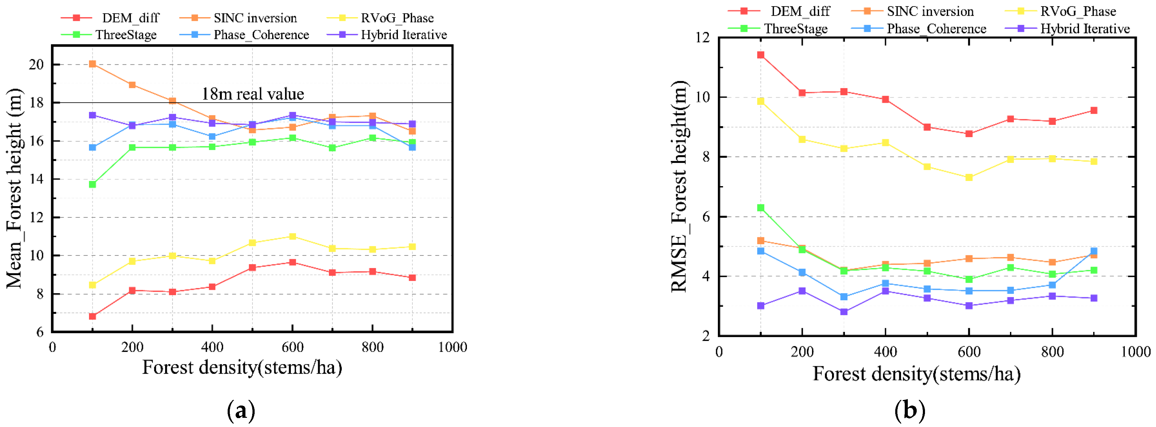
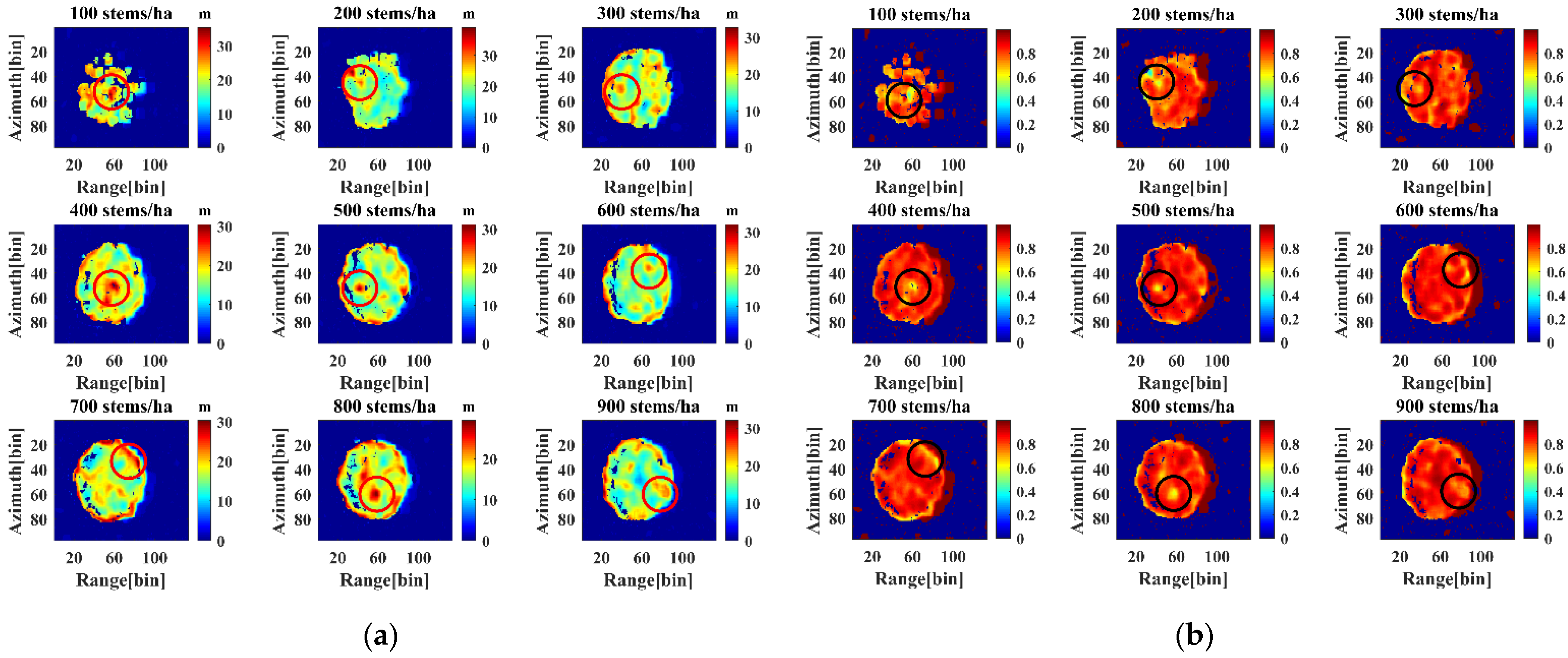
4.1. Results of the Forest Height Inversion for the Simulated Dataset

Simulation of the forest height inversion was performed under ideal conditions where nine groups of stands with various forest densities and a mean tree height of 18 m were utilized. HV polarization represents the volume scattering complex coherence $w_v$, and HH-VV polarization represents the ground scattering complex $w_g$. Comparison experiments used six forest inversion methods.

Table 3. Using simulated datasets of 100–900 stems/ha, six forest height inversion techniques produced forest height and error results.

Forest Density (stems/ha)	100	200	300	400	500	600	700	800	900
DEM Difference Method
MEAN	6.82	8.18	8.10	8.36	9.38	9.64	9.10	9.167	8.84
RMSE	11.41	10.15	10.19	9.93	8.99	8.78	9.27	9.19	9.56
SINC Inversion Method
MEAN	20.04	18.94	18.09	17.16	16.56	16.72	17.25	17.31	16.52
RMSE	5.19	4.94	4.20	4.40	4.43	4.59	4.63	4.46	4.72
RVoG Ground Phase Method
MEAN	8.46	9.70	9.97	9.73	10.66	11.01	10.37	10.32	10.47
RMSE	9.87	8.59	8.28	8.48	7.67	7.31	7.92	7.94	7.84
Three-Stage Inversion Method
MEAN	13.73	15.65	15.66	15.69	15.93	16.16	15.63	16.15	15.92
RMSE	6.30	4.90	4.19	4.28	4.17	3.900	4.30	4.07	4.21
Phase and Coherence Inversion Method
MEAN	15.66	16.86	16.87	16.24	16.87	17.22	16.79	16.80	15.66
RMSE	4.85	4.13	3.32	3.76	3.57	3.51	3.53	3.71	4.85
Coherence amplitude and three-stage hybrid iteration method
MEAN	17.35	16.79	17.23	16.92	16.85	17.36	16.99	16.96	16.88
RMSE	3.01	3.52	2.81	3.50	3.27	3.01	3.19	3.34	3.27

and Figure 8 show each algorithm’s performance and the specific statistical results.

Out of the six inversion algorithms used in the inversion of forest height, the DEM difference method (red line) and RVoG ground phase method (yellow line) performed the worst. Both phase difference algorithms significantly underestimated forest height in sparsely vegetated areas with forest density below 400 stems/ha. The inversion error decreased once the forest density exceeded 400 stems/ha, but the RMSE was consistently greater than 1/3 of the actual tree height. Figure 9 displayed the relative height of the DEM difference method and RVoG ground phase method, respectively. The canopy phase center gradually moved toward the top of the canopy, and the ground phase center also slowly increased. The HV phase center improvement rate was higher than HH-VV polarization in 100–300 stems/ha, and the inversion accuracy was gradually improved. However, when the stand density exceeds 600 stems/ha, the forest gap area decreases, and the canopy phase center no longer increases at this point. The HV and HH-VV polarization phase center heights are also slowly saturated at this point. As a result, the DEM differential method and RVoG ground phase method are subsequently saturated. It also suggested that in sparsely vegetated regions, the canopy phase and ground phase separations represented by HV polarization and HH-VV polarization practically fail, significantly impacting the algorithm’s performance.

The orange line represented the SINC inversion method. The overestimation of this algorithm was apparent when the forest density was below 400 stems/ha. However, the RMSE gradually decreased as the forest density increased and always maintained the RMSE at less than 30% of the actual height. The SINC inversion method ignored the effect of ground phase information on the tree height inversion. As a result, the magnitude impacted the effectiveness of the SINC inversion method. One of the significant characteristics of the SINC inversion method is that the average magnitude is inversely related to the tree height. Figure 10 displayed two-dimensional images of tree height and amplitude representing the canopy polarization channel. When the stand density is low, the amplitude of the HV polarization is small, and the forest height inversion is high. The amplitude of HV polarization increases as the forest density approaches 400 stems/ha, and the forest height inversion error gradually decreases. However, as the forest density increases further, the amplitude of HV polarization reaches the saturation state, which limits the SINC inversion method’s ability to invert and causes the forest height inversion error to fluctuate steadily.

At stand densities lower than 400 stems/ha, the traditional three-stage inversion method (green line) demonstrated a significantly high forest height RMSE. In particular, the forest height was greatly overestimated in the sparse forest stand scenarios below 200 stems/ha, and the error was greater than 30% of the actual forest height. With an increase in forest density, the three-stage inversion method’s advantage was gradually more apparent, and the RMSE was below 25% of the actual measurement. The sparse vegetation broke the assumption of a random homogeneous medium, preventing the RVoG model from exploiting it. On the other hand, the pure canopy phase incorporates a portion of the ground component, causing mistakes in the calculated ground phase.

The inversion error of the phase and coherence inversion method (blue line) was smaller than in the four approaches for low stand density situations. However, the RMSE of this approach was much greater than that of the other four methods at sufficiently high stand density. The main reason was that the results of the SINC inversion method and the RVoG ground phase method were stable enough but increased data redundancy.

The coherence magnitude and three-stage hybrid iterative method (purple line) had significantly better inversion effects under various forest densities when compared to the other five commonly used algorithms. The model’s inversion effect was stable without apparent overestimation or underestimation. The inversion error was about 15% of the actual forest height under both sparse and dense vegetation. In a forest stand with 100 stems/ha, the inversion height was 17.3507 m, and the RMSE was 3.014 m, overcoming the drawbacks of the SINC inversion method and the three-stage inversion method, which fail at low stand densities. The forest height RMSE was 0.5–1 m lower than the phase and coherence inversion method and 1–3 m lower than the three-stage inversion method.

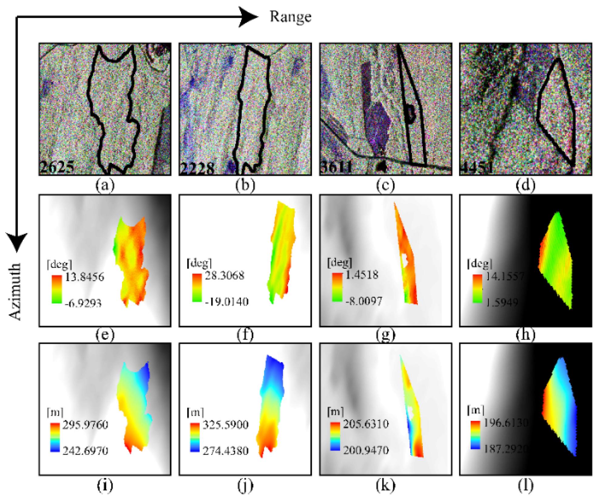
4.2. Results of Forest Height Inversion for a Real Dataset

Considering that the forest conditions in the simulated dataset were ideal, the algorithm was applied to four forest stands in the BioSAR 2008 L-band dataset in this study to test the applicability of the improved method in actual data. The real dataset had four forest stands with a forest density of 628.66 stems/ha, 840.34 stems/ha, 1149.10 stems/ha, and 1330.54 stems/ha. Since the actual forest height was often lower than the field measurement of stand tree height, the Laser-100th was used as the actual forest height for model inversion in this work.

Table 4. The forest density and height of four realistic scenario forest stands. The mean height was measured manually in the field, and the mean height from Lidar is Laser-100th.

Forest Stand Number	Forest Density (stems/ha)	Mean Height (m)	Mean Height from Lidar (m)
4451	628.66	18.72	20.99
2625	840.34	18.06	22.45
3611	1149.10	17.36	21.44
2228	1330.54	17.69	20.50

displays the forest density, average stand height measured in the field, and average laser radar stand height for the four stands.

The algorithm’s performance was affected by the terrain fluctuations in the area covered by the airborne data. So, the hybrid iterative theoretical model used the terrain correction to determine the coherence magnitude and three-stage hybrid iterative application model (Equation (22)), which was then applied to the BioSAR 2008 L-band data. This study introduced the PD coherence optimization approach to enhance the conventional fitting method. ${\gamma }_{P{D}_{HIGH}}$ and ${\gamma }_{P{D}_{LOW}}$ represented the two ends of the long axis of the coherence region, which were used in linear fitting to improve ground phase inversion accuracy. For the inversion of forest height, the pure volume complex coherence after elimination of the ground phase, the terrain-corrected vertical wavenumber, and the local incidence angle were concurrently input into the SINC Inversion Method and the terrain-corrected LUT.

Table 5. Coherence magnitudes and three-stage hybrid iterative application model inversion outcomes for four realistic forest stands. The hybrid iterative algorithm height results from the coherence magnitude and three-stage hybrid iterative application model.

Forest Stand Number	Forest Density (stems/ha)	Hybrid Iterative Algorithm Height (m)	RMSE (m)	MAPE (%)	STD (m)	VAR
4451	628.66	21.21	1.14	3.99	1.11	1.22
2625	840.34	22.19	1.60	6.20	1.05	1.11
3611	1149.10	21.54	1.83	5.86	1.83	3.34
2228	1330.54	20.89	2.17	7.70	1.51	2.27

displays the results of their forest inversion.

The method partially addressed the effects of terrain slope and forest density on the single-baseline PolInSAR inversion and produced good inversion results for all four stands. The standard deviations were all controlled at about 1.5 m, ensuring slight fluctuation when the method was applied to stands with different forest densities. Figure 11 displays the inversion results for the four forest stands. As the forest density increased, the present method was found to progressively raise the RMSE. However, the RMSE < 3 m was not noticeably overestimated or underestimated. In particular, the RMSE was 1.14 m, and the error was lower when the stand density was 628.66 stems/ha. The present technique will be extended from the stand scale to a broader region to estimate forest height inversion, biomass, and carbon stock information across a greater area.

5. Discussion

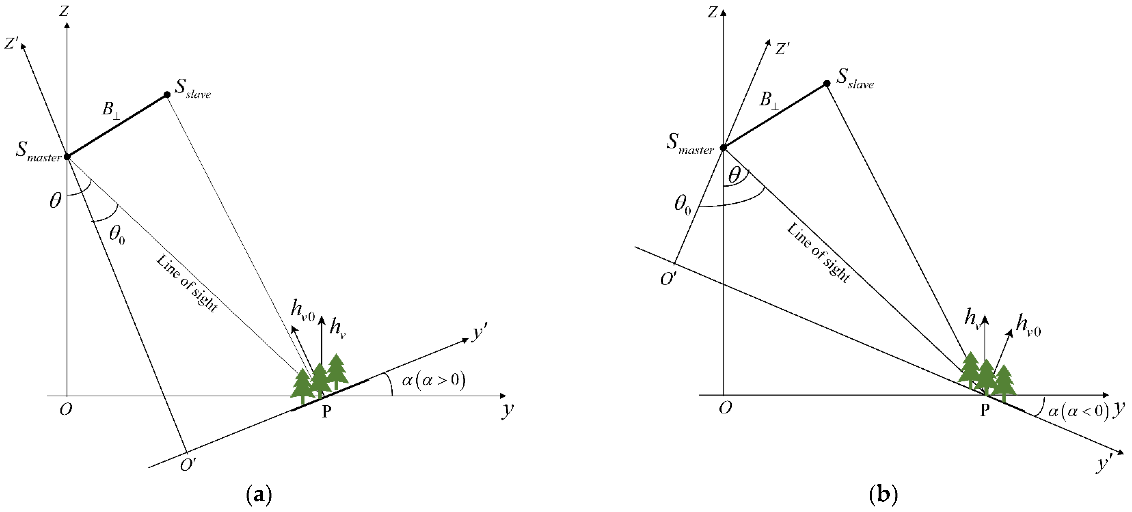
5.1. Effect of Forest Density on Phase

The relative height of the ground phase centers for the RVoG ground phase method was significantly lower than the DEM difference method as illustrated in Figure 9a,b. The phase separation was more significant in the RVoG ground phase method than in the DEM difference method. Figure 12 shows the ground phase error bar of the DEM difference method and RVoG ground phase method, respectively. However, when the stand density exceeds 600 stems/ha, the standard deviation of the ground phase center gradually rises. The HV and HH-VV polarization phase center heights also slowly saturated (Figure 9). As a result, the ground phase is no longer accurately represented by HH-VV.

In general, the height of the volume scattering phase center steadily rises with increasing forest density at the top of the canopy until the saturation of the polarization channel that represents volume scattering. The center height of the ground phase of the DEM difference method or the RVoG ground phase method gradually rises to saturation as the density of the forest stand increases. Improving the precision of forest height inversion is however difficult to achieve since accurate estimation of ground phase in high-density stands is often a challenge. This is because the increase in stand density causes an increase in ground phase inaccuracy. Although the ground phase error in low-density stands is low, the distance between the canopy phase center and the ground phase center is too close, making it impossible to efficiently discern between the two. As such, increasing the accuracy of forest height inversion is quite a challenge.

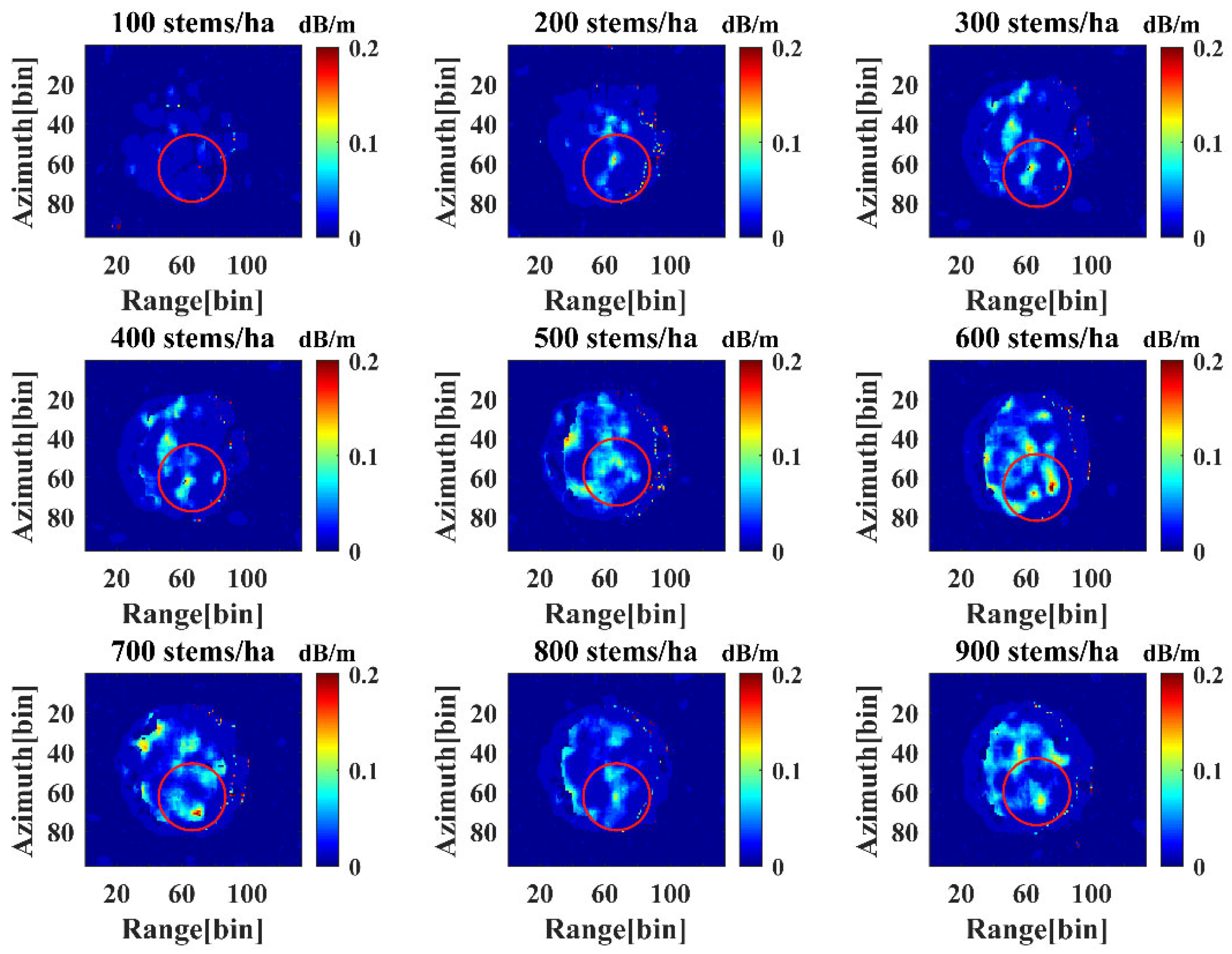
5.2. Effect of Forest Density on the Magnitude

The SINC inversion method is typically a case where the extinction coefficient is 0, as shown by the black line in Figure 13a. The average extinction coefficient depends on the wavelength and the characteristics of the medium (such as height and density). When the signal frequency is fixed, the average extinction coefficient rises, indicating the existence of an effective scattering layer at the top of the bulk layer that attenuates the signal and causes a decrease in penetration depth. As a result, the average extinction coefficient and penetration depth are inversely proportional [39]. The relationship between the volume coherence and the average extinction coefficient is shown in Figure 13b. The volume coherence increases gradually for a fixed tree height as the average extinction coefficient increases. The volume layer is confined into a small space at the top of the volume, indicating a relationship between the volume coherence and the penetration depth. Volume coherence increases with increasing extinction coefficient, while penetration depth in the volume layer decreases. Figure 13c illustrates the relationship between phase, tree height, and extinction coefficient. As the extinction coefficient increases, the relative height of the phase center gradually rises, and the center of the volume scattering phase slowly moves toward the top of the canopy [8]. Extinction coefficient, volume coherence, and volume scattering phase are therefore related. As the extinction coefficient increases, the volume coherence increases, the volume scattering phase increases, while the penetration depth decreases.

Forest density is one of the forest features. The penetration and attenuation of the signal impacted by the forest density can change the forest stand’s average extinction coefficient. Low forest density causes a wide gap in forest vegetation [40], which allows many electromagnetic wave signals to pass through and reach the ground. It reduces signal attenuation in the volume layer, increases penetration depth, and reduces the extinction coefficient. Figure 14 shows two-dimensional images of nine sets of forest stands’ extinction coefficients, with the red circles at the same location on each set of images. For forest stands with densities of 100 stems/ha and 200 stems/ha, the extinction coefficient of the volume layer is lower as shown in Figure 14. The attenuation of the signal into the stand rises as the stand density grows, the extinction coefficient increases, and the effective volume layer develops at the top of the canopy, impacting the computation of complex coherence. When the density grows from 100 stems/ha to 600 stems/ha, the average extinction coefficient in the red circle increases progressively (Figure 14). However, when the stand density reaches 700–900 stems/ha, the extinction coefficient begins to fluctuate, causing fluctuations in the mean phase and amplitude at higher stand densities.

In summary, for L-band, the forest density impacts the inversion of forest height by influencing the extinction coefficient. The effect of the extinction coefficient on the inversion process is reflected in both amplitude and phase. When the stand density is low, the extinction coefficient within the stand is also low. The volume scattering contains a significant ground scattering contribution, and the incomplete separation of the volume phase and ground phase invalidates the forest height method. The extinction coefficient inside the stand increases as stand density rises, the amplitude and phase saturation threshold increases, the distance between ground and canopy phases gradually widens, and the forest height inversion error gradually reduces. When the stand density is high enough, the amplitude and phase tend to saturate. The accuracy of the ground phase estimation influences the accuracy of forest height inversion, and the extinction coefficient stops increasing continuously. Single-baseline PolInSAR inversion approaches can employ coherence optimization algorithms (e.g., SVD, PD, MCD) to increase the distance between ground and canopy phases, or they can use an external DTM to choose the correct ground phase [34,41]. These techniques still result in inversion errors for some ground phases, which raise the inversion errors for forest height. The accuracy of the three-stage inversion method has been increased by restricting the extinction coefficient following the signal penetration depth [42]. Additionally, the multi-baseline PolInSAR approach has been used to overcome the RVoG model’s shortcomings by reducing the extinction coefficient’s impact [42] or applying a tomographic technique to reconstruct the forest height model [43]. These are strategies to overcome the constraints of single-baseline PolInSAR forest height inversion due to factors such as forest density.

5.3. Discussion of Coherence Magnitude and Three-Stage Hybrid Iterative Model

(1) The physical significance of the improved model.

The coherence amplitude and three-stage hybrid iterative model also accounts for the variations in forest density and changes in the extinction coefficient and forest structure. The model is based on the stand density variation, which accounts for the variation in forest structure in relation to stand density. This variation is represented mathematically as the relative error of forest height and physically as the relative height of signal penetration depth. The inversion results are overestimation if $AE$ is negative and underestimated if $AE$ is positive. Higher $\left|AE\right|$ indicates deeper penetration, a lower canopy phase position, and less forest density. The smaller the $\left|AE\right|$, the lower the penetration depth, the higher the canopy phase position, and the denser the forest stand.

$$\begin{array}{ll}AE& =(realvalue-ThreeStage)/realvalue\\ & =1-\frac{ThreeStage}{realvalue}\\ & =\frac{penetrationdepth}{realvalue}\end{array}$$

(20)

When the canopy phase position Y is lower at lower stand densities, the extinction coefficient is lower, and the penetration canopy depth d is larger (Figure 15a). The canopy phase position Y is close to the top of the canopy when the forest density increases. The extinction coefficient is higher, and the penetration canopy depth d is smaller (Figure 15b). Figure 15c depicts the relative errors (penetration depths) for the nine groups of forest stands. At lower forest density, substantial forest gaps emerge, and signal penetration depth under the canopy is high, with relative errors ranging from 0.4 to 0.8. As forest density increases, the forest gap reduces, forest structure becomes homogeneous, canopy phase reaches the top of the canopy, and the signal penetration depth within the forest gradually declines to a value falling between −0.2 and 0.2.

The coherence magnitude and three-stage hybrid iterative model provides the top of vegetation with the traditional three-stage algorithm replacing the phase term, and compensate for the top height of the canopy compressed by the phase information with the SINC inversion method and canopy penetration depth. Because penetration depth is involved, the coherence magnitude and three-stage hybrid iterative algorithm no longer selects the adjustment factor using fixed empirical parameters. Iterative correction coefficients ${\epsilon }_i$ are selected pixel-by-pixel based on the stand’s features to reduce the tree height inversion error. As a result, the coherence magnitude and three-stage hybrid iterative method is more reliable and compatible with the structural traits of the target forest stands, increasing the accuracy of forest height inversion. The two critical assumptions that the volume coherence is independent of polarization and that the ground-to-volume scattering ratio is zero for the volume scattering complex coherence still place restrictions on the model because it is based on the conventional three-stage inversion method. The model’s applicability to X-band and P-band data still requires particular studies because the signal frequency is also a crucial factor impacting the extinction coefficient.

(2) The structure of the improved model

According to the traditional three-stage inversion method, the ideal coherence region comprises all the complex coherence points (the gray elliptical area in Figure 16). The extinction coefficient is often empirically adjusted as a constant to increase the effectiveness of the whole image inversion, which reduces the number of spirals in the LUT to one (the red circle spiral in Figure 16). The hypothetical pure-volume scattering complex coherence point ${\gamma }_{V-pure}$, indicated by the red dot in Figure 16a, is located on the ellipse’s long axis furthest from the ground phase ${\varphi }_{ground}$. In an ideal situation, finding the closest point (green dot in Figure 16) to ${\gamma }_{V-pure}$ in the LUT should yield suitable tree height and extinction coefficient values. The distance between ${\gamma }_{V-pure}$ and ${\gamma }_{V-ideal}$ becomes too large when the coherence region is too distant from the LUT or if the coherence region’s long axis is not long enough. It means ${\gamma }_{V-wrong}$ (the blue dots in Figure 16b) is closer to ${\gamma }_{V-pure}$ than ${\gamma }_{V-ideal}$, which causes a significant under- or overestimation of forest height.

The above ambiguous solutions happen when the ground phase has made an incorrect selection, or the separation between the ground phase and canopy phase is insufficient. For example, in realistic situations with sparse vegetation, overly low extinction coefficients lead to poor coherence and affect the inversion of the LUT. The single-baseline PolInSAR technique, with its simple algorithm, is ineffective, but the multi-baseline PolInSAR approach is complex and requires numerous sets of data input. And the coherent magnitude and three-stage hybrid iterative model uses the penetration depth to alter the weighting factors of pixels to make the overall model more robust. A balance is struck between the simplicity and the validity of the model.

Although the coherence magnitude and three-stage hybrid iterative application model is adjusted for terrain effects, there is still a need to evaluate whether temporal decoherence can be used in the present study’s technique. Temporal decoherence affects forest stands in various ways. The level of landform disturbance varies in PolInSAR data with different temporal baselines [9,20,44]. For various frequencies or various temporal baselines, many temporal decoherence techniques have been developed [19,21,22,23]. The impact of temporal decoherence on various forest densities or stand structures varies [45]. There is currently no standardized algorithm to achieve tree height inversion for all forest densities and all temporal baselines. As a result, data characteristics and forest features need to be considered to execute temporal decoherence correction for the coherence magnitude and three-stage hybrid iterative model.

6. Conclusions

Forest density affects signal penetration and attenuation, leading to the change of extinction coefficient and penetration depth, which affects the inversion performance of the traditional forest height models. When the forest density is sparse, the forest is no longer a uniform medium, and the inversion error is more significant. With the increase in forest density, the inversion error decreases. When the forest density is enormous, the extinction coefficient no longer increases continuously. At this time, the amplitude and phase of the electromagnetic wave are saturated, and the inversion error will increase. Meanwhile, many forest gaps within the forest affect signal penetration, extinction coefficient, and penetration depth.

The coherence magnitude and three-stage hybrid iterative model solves the problem of forest height inversion failure in low forest density regions. It quantifies the penetration depth of different forest stands and compensates for the compression at the top of the canopy. The inversion results do not have significant overestimation or underestimation. The coherence magnitude and three-stage hybrid iterative model can achieve high precision inversion of various forest densities at the stand scale and overcome the underestimation effect of low forest density on the traditional model.

In future work, we intend to will extend the model from the stand scale to a larger scale and realize the high-precision inversion of various forest densities at large scales. The coherence magnitude and three-stage hybrid iterative model introduce the terrain correction algorithm. However, the correction of temporal decoherence must consider the radar frequency, temporal resolution, and other system parameters and stand characteristics. The fusion of the temporal decoherence correction algorithm and the improved algorithm in this paper will also be considered in future work. Nevertheless, the proposed method is simple, robust, and easy to extend, which addresses the failure problems associated with traditional inversion methods in sparse forest areas.

References

1. Ghasemi, N.; Sahebi, M.R.; Mohammadzadeh, A. A Review on Biomass Estimation Methods Using Synthetic Aperture Radar Data. Int. J. Geomat. Geosci. 2011, 1, 776–788. [Google Scholar]
2. Mora, B.; Wulder, M.A.; White, J.C.; Hobart, G. Modeling Stand Height, Volume, and Biomass from Very High Spatial Resolution Satellite Imagery and Samples of Airborne LIDAR. Remote Sens. 2013, 5, 2308–2326. [Google Scholar] [CrossRef] [Green Version]
3. Cao, C.; Bao, Y.; Xu, M.; Chen, W.; Zhang, H.; He, Q.; Li, Z.; Guo, H.; Li, J.; Li, X.; et al. Retrieval of Forest Canopy Attributes Based on a Geometric-Optical Model Using Airborne LiDAR and Optical Remote-Sensing Data. Int. J. Remote Sens. 2012, 33, 692–709. [Google Scholar] [CrossRef]
4. Wenxue, F.; Huadong, G.; Xinwu, L.; Bangsen, T.; Zhongchang, S. Extended Three-Stage Polarimetric SAR Interferometry Algorithm by Dual-Polarization Data. IEEE Trans. Geosci. Remote Sens. 2016, 54, 2792–2802. [Google Scholar] [CrossRef]
5. Askne, J.I.H.; Ulander, L.M.H.; Soja, M.J. Biomass Estimation in a Boreal Forest from TanDEM-X Data, Lidar DTM, and the Interferometric Water Cloud Model. Remote Sens. Environ. 2017, 196, 265–278. [Google Scholar] [CrossRef]
6. Treuhaft, R.N.; Madsen, S.N.; Moghaddam, M.; Zyl, J.J. Van Vegetation Characteristics and Underlying Topography from Interferolnetric Radar. Radio Sci. 1996, 31, 1449–1485. [Google Scholar] [CrossRef]
7. Denbina, M.; Simard, M.; Hawkins, B. Forest Height Estimation Using Multibaseline PolInSAR and Sparse Lidar Data Fusion. IEEE J. Sel. Top. Appl. Earth Obs. Remote Sens. 2018, 11, 3415–3433. [Google Scholar] [CrossRef]
8. Cloude, S.R. Polarimetric Sar Interferometry. IEEE Trans. Geosci. Remote Sens. 1998, 36, 1551–1565. [Google Scholar] [CrossRef]
9. Askne, J.I.H.; Dammert, P.B.G.; Ulander, L.M.H.; Smith, G. C-Band Repeat-Pass Interferometric SAR Observations of the Forest. IEEE Trans. Geosci. Remote Sens. 1997, 35, 25–35. [Google Scholar] [CrossRef]
10. Zhou, Z.B.; Ma, H.Z.; Zhu, X.B.; Sun, L. Comparative Analysis of Forest Height Retrieval Methods by Polarimetric SAR Interferometry. Adv. Mater. Res. 2013, 726–731, 4686–4689. [Google Scholar] [CrossRef]
11. Cloude, S. Polarisation: Applications in Remote Sensing; OUP: Oxford, UK, 2009. [Google Scholar]
12. Cloude, S.R. Polarization Coherence Tomography. Radio Sci. 2006, 41, 1–27. [Google Scholar] [CrossRef]
13. Cloude, S.R.; Papathanassiou, K.P. Three-Stage Inversion Process for Polarimetric SAR Interferometry. IEE Proc.-Radar Sonar Navig. 2003, 150, 125–134. [Google Scholar] [CrossRef] [Green Version]
14. Cloude, S.R.; Papathanassiou, K.P. Polarimetric Radar Interferometry. Opt. Sci. Eng. Instrum. 1997, 3120, 224–235. [Google Scholar]
15. Tabb, M.; Orrey, J.; Flynn, T.; Carande, R. Phase Diversity: A Decomposition for Vegetation Parameter Estimation Using Polarimetric SAR Interferometry. In Proceedings of the European Conference on Synthetic Aperture Radar Conference, Cologne, Germany, 4–6 June 2002; pp. 721–724. [Google Scholar]
16. Zhang, Q.; Mercer, J.B.; Cloude, S.R. Forest Height Estimation from Indrex-II L-Band Polarimetric InSAR Data. In Proceedings of the International Archives of the Photogrammetry, Remote Sensing and Spatial Information Sciences, Beijing, China, 3–11 July 2008. [Google Scholar]
17. Zebker, H.A.; Villasenor, J. Decorrelation in Interferometric Radar Echoes. IEEE Trans. Geosci. Remote Sens. 1992, 30, 950–959. [Google Scholar] [CrossRef] [Green Version]
18. Ulander, L.M.H. Radiometric Slope Correction of Synthetic-Aperture Radar Images. IEEE Trans. Geosci. Remote Sens. 1996, 34, 1115–1122. [Google Scholar] [CrossRef]
19. Sun, X.; Wang, B.; Xiang, M.; Fu, X.; Zhou, L.; Li, Y. S-RVoG Model Inversion Based on Time-Frequency Optimization for P-Band Polarimetric SAR Interferometry. Remote Sens. 2019, 11, 1033. [Google Scholar] [CrossRef] [Green Version]
20. Lu, H.; Suo, Z.; Guo, R.; Bao, Z. S-RVoG Model for Forest Parameters Inversion over Underlying Topography. Electron. Lett. 2013, 49, 618–620. [Google Scholar] [CrossRef]
21. Xie, Q.; Zhu, J.; Wang, C.; Fu, H.; Lopez-Sanchez, J.M.; Ballester-Berman, J.D. A Modified Dual-Baseline PolInSAR Method for Forest Height Estimation. Remote Sens. 2017, 9, 819. [Google Scholar] [CrossRef] [Green Version]
22. Papathanassiou, K.P.; Cloude, S.R. The Effect of Temporal Decorrelation on the Inversion of Forest Parameters from Polinsar Data. Int. Geosci. Remote Sens. Symp. 2003, 3, 1429–1431. [Google Scholar] [CrossRef]
23. Lee, S.K.; Kugler, F.; Papathanassiou, K.P.; Hajnsek, I. Quantifying Temporal Decorrelation over Boreal Forest at L- And P-Band. In Proceedings of the 7th European Conference on Synthetic Aperture Radar, Friedrichshafen, Germany, 2–5 June 2008. [Google Scholar]
24. Lavalle, M.; Simard, M.; Pottier, E.; Solimini, D. PolInSAR Forestry Applications Improved by Modeling Height-Dependent Temporal Decorrelation. In Proceedings of the 2010 IEEE International Geoscience and Remote Sensing Symposium, Honolulu, HI, USA, 25–30 July 2010; pp. 4772–4775. [Google Scholar]
25. Lei, Y.; Siqueira, P. Estimation of Forest Height Using Spaceborne Repeat-Pass L-Band InSAR Correlation Magnitude over the US State of Maine. Remote Sens. 2014, 6, 10252–10285. [Google Scholar] [CrossRef] [Green Version]
26. Lavalle, M.; Simard, M.; Solimini, D.; Pottier, E. Height-Dependent Temporal Decorrelation for POLINSAR and TOMOSAR Forestry Applications. In Proceedings of the 8th European Conference on Synthetic Aperture Radar, Aachen, Germany, 7–10 June 2010; pp. 1–4. [Google Scholar]
27. Qinghua, X.I.E.; Changcheng, W.; Jianjun, Z.H.U.; Haiqiang, F.U. Forest Height Inversion by Combining S-RVOG Model with Terrain Factor and PD Coherence Optimization. Acta Geod. Cartogr. Sin. 2015, 44, 686. [Google Scholar]
28. Garestier, F.; Dubois-Fernandez, P.C.; Papathanassiou, K.P. Pine Forest Height Inversion Using Single-Pass X-Band PolInSAR Data. IEEE Trans. Geosci. Remote Sens. 2008, 46, 59–68. [Google Scholar] [CrossRef]
29. Wang, C.; Wang, L.; Fu, H.; Xie, Q.; Zhu, J. The Impact of Forest Density on Forest Height Inversion Modeling from Polarimetric InSAR Data. Remote Sens. 2016, 8, 291. [Google Scholar] [CrossRef]
30. Pottier, E.; Ferro-Famil, L.; Allain, S.; Cloude, S.R.; Hajnsek, I.; Papathanassiou, K.; Moreira, A.; Williams, M.; Minchella, A.; Lavalle, M. Overview of the PolSARpro v4. 0 Software New Updates of the Educational Toolbox for Polarimetric and Interferometric Polarimetric SAR Data Processing. In Proceedings of the POLinSAR 2009, Frascati, Italy, 26 January 2009; p. CD-ROM. [Google Scholar]
31. Papathanassiou, K.P.; Cloude, S.R. Single-Baseline Polarimetric SAR Interferometry. IEEE Trans. Geosci. Remote Sens. 2001, 39, 2352–2363. [Google Scholar] [CrossRef] [Green Version]
32. Hajnsek, I.; Scheiber, R.; Keller, M.; Horn, R.; Lee, S.; Ulander, L.; Gustavsson, A.; Sandberg, G.; Le Toan, T.; Tebaldini, S. BIOSAR 2008: Final Report; ESA-ESTEC: Noordwijk, Netherlands, 2009; Volume 22052. [Google Scholar]
33. Neumann, M.; Neumann, M.; De, T.; Neumann, M. Remote Sensing of Vegetation Using Multi-Baseline Polarimetric SAR Interferometry: Theoretical Modeling and Physical Parameter Retrieval. Ph.D. Thesis, Université Rennes, Rennes, France, 2009. [Google Scholar]
34. Soja, M.J.; Sandberg, G.; Ulander, L.M.H. Regression-Based Retrieval of Boreal Forest Biomass in Sloping Terrain Using P-Band SAR Backscatter Intensity Data. IEEE Trans. Geosci. Remote Sens. 2012, 51, 2646–2665. [Google Scholar] [CrossRef] [Green Version]
35. Yamada, H.; Yamaguchi, Y.; Rodriguez, E.; Kim, Y.; Boerner, W.M. Polarimetric SAR Interferometry for Forest Canopy Analysis by Using the Super-Resolution Method. In Proceedings of the 2001 International Geoscience and Remote Sensing Symposium (Cat. No. 01CH37217), Sydney, NSW, Australia, 9–13 July 2001; Volume 3, pp. 1101–1103. [Google Scholar]
36. Mette, T.; Kugler, F.; Papathanassiou, K.; Hajnsek, I. Forest and the Random Volume over Ground-Nature and Effect of 3 Possible Error Types. In Proceedings of the European Conference on Synthetic Aperture Radar (EUSAR), Dresden, Germany, 16–18 May 2006; pp. 1–4. [Google Scholar]
37. Mao, Y.; Michel, O.O.; Yu, Y.; Fan, W.; Sui, A.; Liu, Z.; Wu, G. Retrieval of Boreal Forest Heights Using an Improved Random Volume over Ground (RVoG) Model Based on Repeat-Pass Spaceborne Polarimetric SAR Interferometry: The Case Study of Saihanba, China. Remote Sens. 2021, 13, 4306. [Google Scholar] [CrossRef]
38. Liao, Z.; He, B.; Quan, X.; van Dijk, A.I.J.M.; Qiu, S.; Yin, C. Biomass Estimation in Dense Tropical Forest Using Multiple Information from Single-Baseline P-Band PolInSAR Data. Remote Sens. Environ. 2019, 221, 489–507. [Google Scholar] [CrossRef]
39. Managhebi, T.; Maghsoudi, Y.; Zoej, M.J.V. An Improved Three-Stage Inversion Algorithm in Forest Height Estimation Using Single-Baseline Polarimetric Sar Interferometry Data. IEEE Geosci. Remote Sens. Lett. 2018, 15, 887–891. [Google Scholar] [CrossRef]
40. Liu, F.; Yang, Z.; Zhang, G. Canopy Gap Characteristics and Spatial Patterns in a Subtropical Forest of South China after Ice Storm Damage. J. Mt. Sci. 2020, 17, 1942–1958. [Google Scholar] [CrossRef]
41. Zhang, J.; Zhang, Y.; Fan, W.; He, L.; Yu, Y.; Mao, X. A Modified Two-Steps Three-Stage Inversion Algorithm for Forest Height Inversion Using Single-Baseline L-Band PolInSAR Data. Remote Sens. 2022, 14, 1986. [Google Scholar] [CrossRef]
42. Cloude, S.R.; Williams, M.L. A Coherent EM Scattering Model for Dual Baseline POLInSAR. In Proceedings of the IGARSS 2003. 2003 IEEE International Geoscience and Remote Sensing Symposium. Proceedings (IEEE Cat. No. 03CH37477), Toulouse, France, 21–25 July 2003; Volume 3, pp. 1423–1425. [Google Scholar]
43. Tebaldini, S.; Rocca, F. Multibaseline Polarimetric SAR Tomography of a Boreal Forest at P-and L-Bands. IEEE Trans. Geosci. Remote Sens. 2011, 50, 232–246. [Google Scholar] [CrossRef]
44. Rocca, F. Modeling Interferogram Stacks. IEEE Trans. Geosci. Remote Sens. 2007, 45, 3289–3299. [Google Scholar] [CrossRef]
45. Simard, M.; Hensley, S.; Lavalle, M.; Dubayah, R.; Pinto, N.; Hofton, M. An Empirical Assessment of Temporal Decorrelation Using the Uninhabited Aerial Vehicle Synthetic Aperture Radar over Forested Landscapes. Remote Sens. 2012, 4, 975–986. [Google Scholar] [CrossRef]
Figure 1. Scenarios of simulation for nine groups of simulated data. The reference height for all nine datasets is 18 m. Forest density ranges from 100 to 900 stems/ha.
Remotesensing 15 00081 g001
Figure 2. Pauli-basis (HV, HH + VV, and HH − VV) composite images of nine simulated data sets.
Remotesensing 15 00081 g002
Figure 3. The extent of the study area and the several products included in the BioSAR 2008 dataset. (a) The red pentagram in the upper right corner of the thumbnail depicts the location of the study area in Sweden. The red rectangle region shows the SAR image. The green and yellow polygons represent the 31 forest stands in the red rectangle region; the four yellow polygons represent the forest stands employed in this study. (b) The green background image is a Lidar image with a grid size resampling of 1 m × 1 m. Pauli-basis image is the extent of SAR images. The Pauli-basis image (on the left) shows the locations of the four forest stands. The shape of four forest stands on the Pauli-basis image is shown on the right. All products on the map are geocoded to WGS84 UTM Zone 34N.
Remotesensing 15 00081 g003
Figure 4. Flow chart. DEM_diff is the DEM difference method, SINC inversion is the SINC inversion method, RVoG_Phase represents the RVoG ground phase method, ThreeStage represents the traditional three-stage inversion method, Phase_Coherence is the phase and coherence inversion method, Hybrid Iterative Method (theoretical model) represents coherence amplitude and three-stage hybrid iterative theoretical model. The hybrid Iterative Method (application model) describes the coherence amplitude and three-stage hybrid iterative application model.
Remotesensing 15 00081 g004
Figure 5. Schematic representation of the RVoG two-layer scattering model. The two-layer model consists of a volume layer and a ground layer, where the volume layer is supposed to be a medium with uniform random density.
Remotesensing 15 00081 g005
Figure 6. The geometric model of forest scattering is affected by terrain slope. (a) The landscape distribution faces the radar sensor when the terrain slope is positive. (b) When the terrain slope is negative, the landscape distribution is at the back of the radar sensor. y o z and y o z are the coordinate system under flat terrain and the slope-corrected coordinate system, respectively. B means the vertical baseline. S m a s t e r and S s l a v e are the master image and the slave image, respectively. P is the ground object (e.g., forest), θ is the radar incidence angle, θ 0 is the local incidence angle, α is the range slope, h v 0 is the slope-corrected forest height under the y o z coordinate system, and h v is the forest height under the y o z coordinate system.
Remotesensing 15 00081 g006
Figure 7. Images of the four forest stands’ terrain slope and DEM. (ad) Pauli-basis of four stands in the SAR coordinate system. (eh) Terrain slope (il) DEM.
Remotesensing 15 00081 g007
Figure 8. Results graphs for the six forest height inversion techniques for simulated data sets with 100–900 stems/ha. (a) Line graph of forest height (b) Line graph of forest height error. The red line means the DEM difference method (DEM_diff), and the orange line represents the SINC inversion method (SINC inversion). The yellow line describes the RVoG ground phase method (RVoG_Phase), and the green line represents the traditional three-stage inversion method (ThreeStage). The blue line is the phase and coherence inversion method (Phase_Coherence), and the purple line represents the coherence magnitude and three-stage hybrid iterative method (Hybrid Iterative).
Remotesensing 15 00081 g008
Figure 9. Relative heights of canopy phase center and ground phase center. (a) DEM difference method (b) RVoG ground phase method.
Remotesensing 15 00081 g009
Figure 10. In the SINC inversion method, two-dimensional images of tree height and HV polarization intensity are generated for nine groups of forest stands. (a) A two-dimensional map of forest height for nine groups of forest stands. (b) A two-dimensional map of the HV magnitude for nine groups of forest stands. For each of the nine groups of forest stands, the black circles indicate the regions with low amplitude values. The red and black circles are positioned in the same location in both images.
Remotesensing 15 00081 g010
Figure 11. Forest height mapping in four forest stands was accomplished using coherence magnitude and three-stage hybrid iterative application algorithms. (a) Stand 2625, (b) stand 2228, (c) stand 3611, and (d) stand 4451.
Remotesensing 15 00081 g011
Figure 12. Error bar plot of ground phase center relative heights. (a) DEM difference method (b) RVoG ground phase method.
Remotesensing 15 00081 g012
Figure 13. A presentation of the relationship between extinction coefficient, coherence amplitude, and phase. (a) The relationship between complex coherence and extinction coefficient in the complex unit circle. (b) The relationship between tree height, amplitude, and extinction coefficient. (c) The relationship between extinction coefficient and phase center height, tree height ( σ = 0   d B / m is the black line, σ = 0.1   d B / m is the blue line, σ = 0.125   d B / m is the yellow line, and σ = 0.5   d B / m is the red line).
Remotesensing 15 00081 g013
Figure 14. The two-dimensional maps depict the extinction coefficients of nine groups of stands inverted using the traditional three-stage inversion method, with red circles representing the same locations of the nine groups of forest stands.
Remotesensing 15 00081 g014
Figure 15. Diagram showing the relative tree height error, penetration depth, and forest density. (a) Schematic representation of signal penetration at low forest density, where penetration depth d is higher, and canopy phase center Y is lower. (b) Schematic illustration of signal penetration at high forest density showing that the penetration depth d is less and the canopy phase center Y is more elevated and closer to the canopy’s top. (c) The relative error (penetration depth) of the nine groups of forest stand inversions using the traditional three-stage inversion method.
Remotesensing 15 00081 g015
Figure 16. An illustration of ideal geometric structure of the conventional three-stage inversion method and the situation of a failed geometric structure. (a) The ideal geometry of the traditional three-stage inversion method. (b) Either the coherence region’s long axis is too short or too far away from the LUT for the geometric structure to fail.
Remotesensing 15 00081 g016