
Toward Multi-Stage Phenotyping of Soybean with Multimodal UAV Sensor Data: A Comparison of Machine Learning Approaches for Leaf Area Index Estimation

Abstract
:1. Introduction
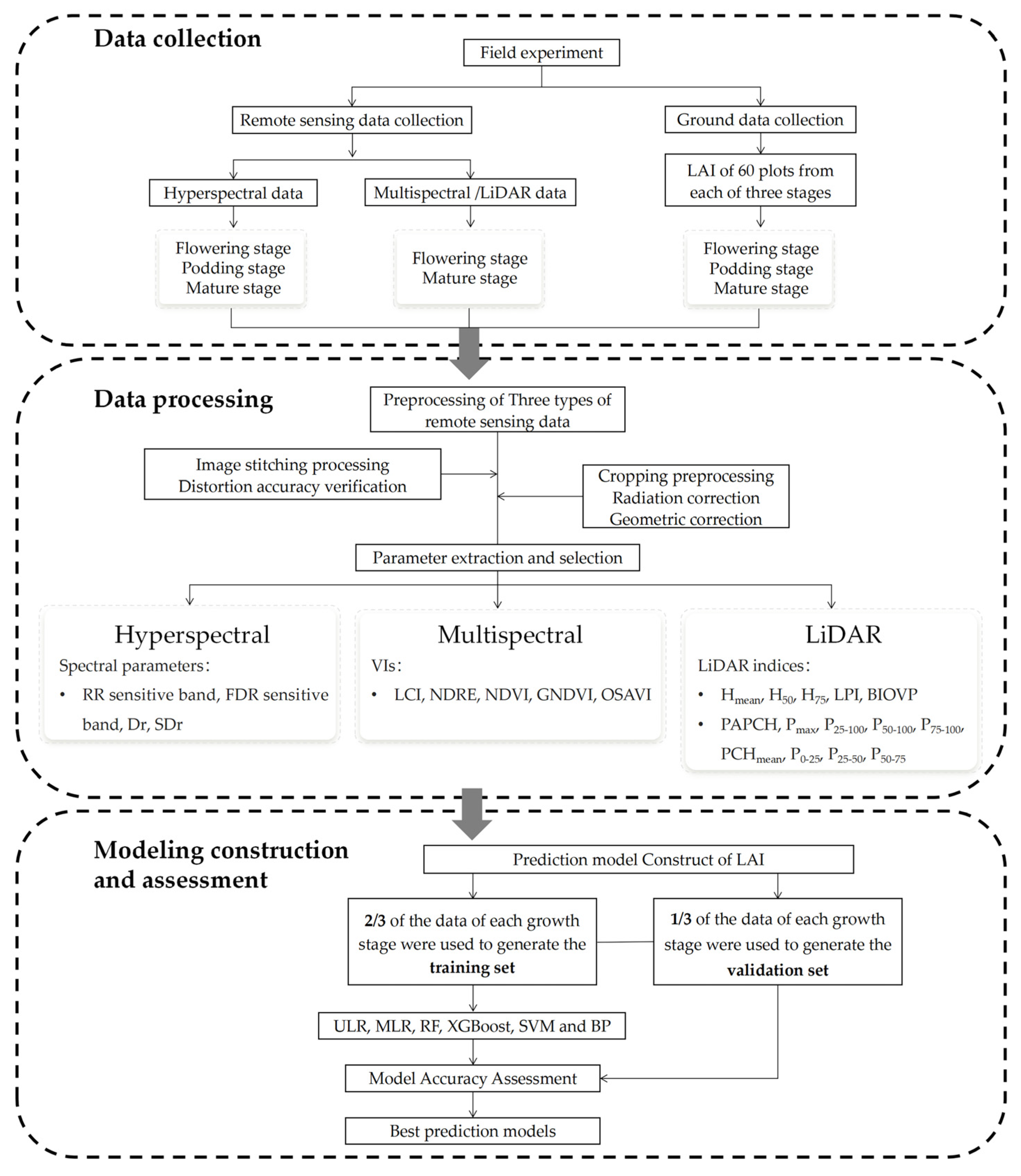
2. Materials and Methods
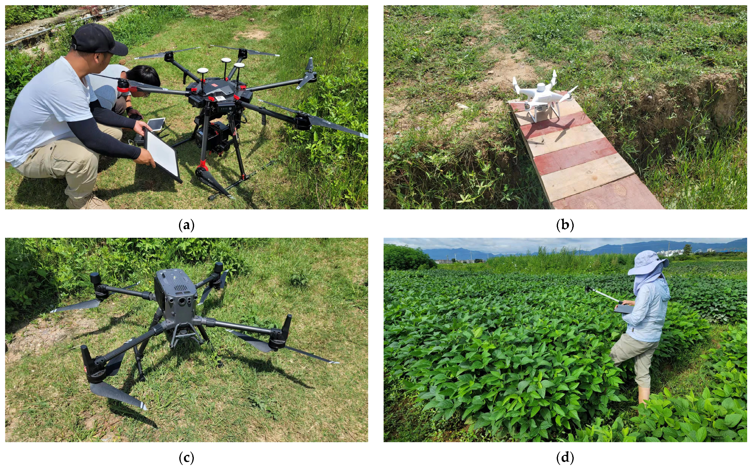
2.1. Field Experiment
2.2. Data Collection
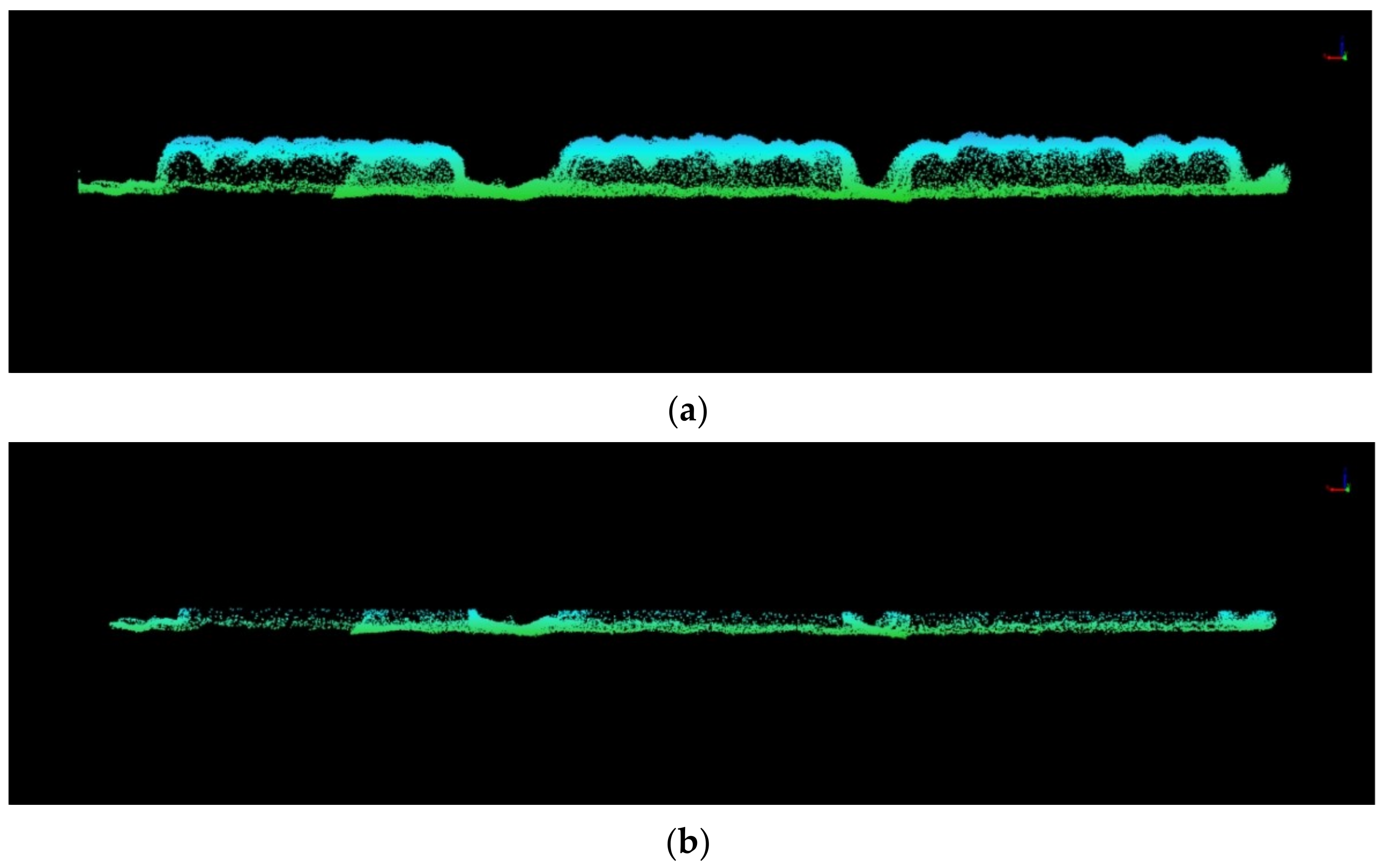
2.3. Data Processing

| Type of Sensor | Modeling Parameters | Description/Formula | References |
|---|---|---|---|
| Hyperspectral | RR sensitive band | The RR band with the highest correlation with LAI | [41] |
| FDR sensitive band | The FDR band with the highest correlation with LAI | [42] | |
| Dr | The value of the first derivative corresponding to the position of the red edge | [38] | |
| SDr | Area enclosed by first derivative spectra in the red-edge range (680nm~760nm) | [38] | |
| Multispectral | LCI | (NIR − RE)/(NIR + R) 1 | [43] |
| NDRE | (NIR − RE)/(NIR + RE) 1 | [44] | |
| NDVI | (NIR − R)/(NIR + R) 1 | [45] | |
| GNDVI | (NIR − G)/(NIR + G) 1 | [46] | |
| OSAVI | (1 + 0.16)(NIR − R)/(NIR + R + 0.16) 1 | [47] | |
| LiDAR | Hmean | 2 | [48] |
| H50 | 2 | [48] | |
| H75 | 2 | [48] | |
| LPI | 3 | [49] | |
| BIOVP | 4 | [50] | |
| PAPCH | The percentage of point clouds above the average point cloud height in the total number of point clouds | - | |
| Pmax | The height with the largest number of point clouds was extracted and the percentage of the number of point clouds at this height | - | |
| P25–100 | The percentage of 25%~100% Height Point Cloud | - | |
| P50–100 | The percentage of 50%~100% Height Point Cloud | - | |
| P75–100 | The percentage of 75%~100% Height Point Cloud | - | |
| PCHmean | The percentage of the average Point Cloud Height | - | |
| P0–25 | The percentage of 0%~25% Height Point Cloud | - | |
| P25–50 | The percentage of 25%~50% Height Point Cloud | - | |
| P50–75 | The percentage of 50%~75% Height Point Cloud | - |
2.4. Machine Learning Methods
2.5. Model Accuracy Assessment
3. Results
3.1. Prediction Models of LAI Based on Hyperspectral Data
3.1.1. Modeling Parameter Selection
3.1.2. Prediction Models of LAI Constructed by Different Algorithms
3.1.3. Comparison of Prediction Models Constructed by Different Algorithms
3.1.4. Universal Model of LAI for Multiple Growth Stages
3.2. Prediction Models of LAI Based on Multispectral Data
3.3. Prediction Models of LAI Based on LiDAR Data
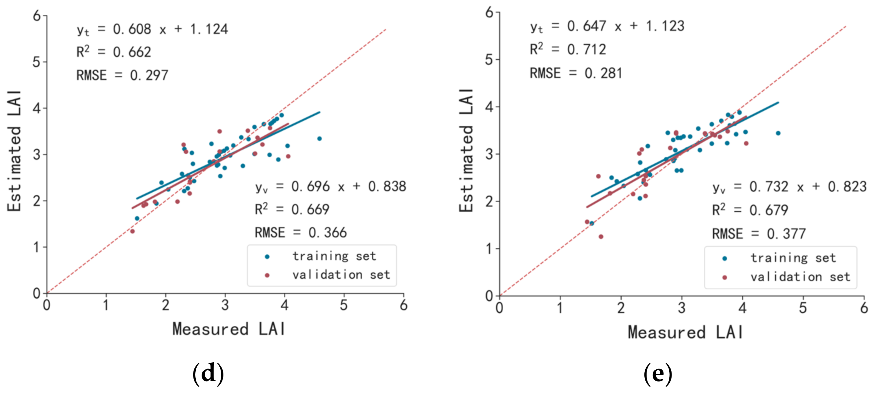
3.4. Prediction Models of LAI Based on Multimodal Data
3.4.1. Prediction Models of LAI by Integrating Three Types of Remote Sensing Data
3.4.2. Prediction Models of LAI by Integrating Hyperspectral and Multispectral Data
4. Discussion
4.1. Parameter Selection for Model Construction of LAI with Different Types of Remote Sensing Data
4.2. Performance Comparison of Three Types of Remote Sensing Data on LAI Prediction
4.3. Models of LAI Constructed with Multimodal Data
4.4. Comparison of Prediction Models of LAI Based on Different Algorithms
4.5. Prediction Models of LAI at Different Growth Stages Based on Hyperspectral Data
5. Conclusions
Author Contributions
Funding
Data Availability Statement
Acknowledgments
Conflicts of Interest
Abbreviations
| UAV | Unmanned Aerial Vehicle |
| LAI | Leaf Area Index |
| AGB | Above-Ground Biomass |
| RR | Raw Reflectance |
| FDR | First Derivative Reflectance |
| REP | Red Edge Position |
| Dr | Red Edge Amplitude |
| SDr | Red Edge Area |
| Drmax | Maximum Red-edge Amplitude |
| Drmin | Minimum Red-edge Amplitude |
| LCI | Land Cover Index |
| OSAVI | Optimized Soil Adjusted Vegetation Index |
| NDVI | Normalized Difference Vegetation Index |
| GNDVI | Green Normalized Difference Vegetative Index |
| NDRE | Normalized Difference Red Edge |
| ROI | Region of Interest |
| CSF | Cloth Simulation Filter |
| TIN | Triangulated Irregular Network |
| DEM | Digital Elevation Model |
| DSM | Digital Surface Model |
| CHM | Canopy Height Model |
| Hmean | Mean Plant Height |
| H50 | 50 Percentile Plant Height |
| H75 | 75 Percentile Plant Height |
| LPI | Laser Penetration Index |
| BIOVP | Three-Dimensional Volumetric Parameters |
| P0–25 | The percentage of 0%~25% height point cloud |
| P25–50 | The percentage of 25%~50% height point cloud |
| P50–75 | The percentage of 50%~75% height point cloud |
| P25–100 | The percentage of 25%~100% height point cloud |
| P50–100 | The percentage of 50%~100% height point cloud |
| P75–100 | The percentage of 75%~100% height point cloud. |
| Pmax | The percentage of the number of point clouds at the height with the largest number of point clouds |
| PCHmean | The percentage of the average point cloud height |
| PAPCH | The percentage of point clouds above the average point cloud height in the total number of point clouds |
| ULR | Unary Linear Regression |
| PLSR | Partial Least Squares Regression |
| MLR | Multivariable Linear Regression |
| RF | Random Forest |
| XGBoost | eXtreme Gradient Boosting |
| SVR | Support Vector Regression |
| SVM | Support Vector Machine |
| ANN | Artificial Neural Network |
| BP | Back Propagation |
| RBF | Radial Basis Function |
| ReLU | Rectified Linear Unit |
References
- Singh, G. The Soybean: Botany, Production and Uses; CABI: Wallingford, UK, 2010. [Google Scholar]
- Bréda, N.J. Ground-based measurements of leaf area index: A review of methods, instruments and current controversies. J. Exp. Bot. 2003, 54, 2403–2417. [Google Scholar] [CrossRef] [Green Version]
- Haboudane, D. Hyperspectral vegetation indices and novel algorithms for predicting green LAI of crop canopies: Modeling and validation in the context of precision agriculture. Remote Sens. Environ. 2004, 90, 337–352. [Google Scholar] [CrossRef]
- Alexandridis, T.K.; Ovakoglou, G.; Clevers, J.G. Relationship between MODIS EVI and LAI across time and space. Geocarto Int. 2020, 35, 1385–1399. [Google Scholar] [CrossRef]
- Yang, G.; Liu, J.; Zhao, C.; Li, Z.; Huang, Y.; Yu, H.; Xu, B.; Yang, X.; Zhu, D.; Zhang, X. Unmanned aerial vehicle remote sensing for field-based crop phenotyping: Current status and perspectives. Front. Plant Sci. 2017, 8, 1111. [Google Scholar] [CrossRef] [Green Version]
- Underwood, J.; Wendel, A.; Schofield, B.; McMurray, L.; Kimber, R. Efficient in-field plant phenomics for row-crops with an autonomous ground vehicle. J. Field Robot. 2017, 34, 1061–1083. [Google Scholar] [CrossRef]
- Pratap, A.; Gupta, S.; Nair, R.M.; Gupta, S.; Schafleitner, R.; Basu, P.; Singh, C.M.; Prajapati, U.; Gupta, A.K.; Nayyar, H. Using plant phenomics to exploit the gains of genomics. Agronomy 2019, 9, 126. [Google Scholar] [CrossRef] [Green Version]
- Feng, D.; Xu, W.; He, Z.; Zhao, W.; Yang, M. Advances in plant nutrition diagnosis based on remote sensing and computer application. Neural Comput. Appl. 2020, 32, 16833–16842. [Google Scholar] [CrossRef]
- Jin, X.; Liu, S.; Baret, F.; Hemerlé, M.; Comar, A. Estimates of plant density of wheat crops at emergence from very low altitude UAV imagery. Remote Sens. Environ. 2017, 198, 105–114. [Google Scholar] [CrossRef] [Green Version]
- Zhang, J.; Huang, Y.; Pu, R.; Gonzalez-Moreno, P.; Yuan, L.; Wu, K.; Huang, W. Monitoring plant diseases and pests through remote sensing technology: A review. Comput. Electron. Agric. 2019, 165, 104943. [Google Scholar] [CrossRef]
- Tao, H.; Feng, H.; Xu, L.; Miao, M.; Long, H.; Yue, J.; Li, Z.; Yang, G.; Yang, X.; Fan, L. Estimation of crop growth parameters using UAV-based hyperspectral remote sensing data. Sensors 2020, 20, 1296. [Google Scholar] [CrossRef]
- Maes, W.H.; Steppe, K. Perspectives for remote sensing with unmanned aerial vehicles in precision agriculture. Trends Plant Sci. 2019, 24, 152–164. [Google Scholar] [CrossRef] [PubMed]
- Berni, J.A.; Zarco-Tejada, P.J.; Suárez, L.; Fereres, E. Thermal and narrowband multispectral remote sensing for vegetation monitoring from an unmanned aerial vehicle. IEEE Trans. Geosci. Remote Sens. 2009, 47, 722–738. [Google Scholar] [CrossRef] [Green Version]
- Yue, J.; Lei, T.; Li, C.; Zhu, J. The application of unmanned aerial vehicle remote sensing in quickly monitoring crop pests. Intell. Autom. Soft Comput. 2012, 18, 1043–1052. [Google Scholar] [CrossRef]
- Hunt, E.R.; Cavigelli, M.; Daughtry, C.S.; Mcmurtrey, J.E.; Walthall, C.L. Evaluation of digital photography from model aircraft for remote sensing of crop biomass and nitrogen status. Precis. Agric. 2005, 6, 359–378. [Google Scholar] [CrossRef]
- Córcoles, J.I.; Ortega, J.F.; Hernández, D.; Moreno, M.A. Estimation of leaf area index in onion (Allium cepa L.) using an unmanned aerial vehicle. Biosyst. Eng. 2013, 115, 31–42. [Google Scholar] [CrossRef]
- Kanning, M.; Kühling, I.; Trautz, D.; Jarmer, T. High-resolution UAV-based hyperspectral imagery for LAI and chlorophyll estimations from wheat for yield prediction. Remote Sens. 2018, 10, 2000. [Google Scholar] [CrossRef] [Green Version]
- Bendig, J.; Bolten, A.; Bennertz, S.; Broscheit, J.; Eichfuss, S.; Bareth, G. Estimating biomass of barley using crop surface models (CSMs) derived from UAV-based RGB imaging. Remote Sens. 2014, 6, 10395–10412. [Google Scholar] [CrossRef] [Green Version]
- Boegh, E.; Soegaard, H.; Broge, N.; Hasager, C.; Jensen, N.; Schelde, K.; Thomsen, A. Airborne multispectral data for quantifying leaf area index, nitrogen concentration, and photosynthetic efficiency in agriculture. Remote Sens. Environ. 2002, 81, 179–193. [Google Scholar] [CrossRef]
- Adão, T.; Hruška, J.; Pádua, L.; Bessa, J.; Peres, E.; Morais, R.; Sousa, J.J. Hyperspectral imaging: A review on UAV-based sensors, data processing and applications for agriculture and forestry. Remote Sens. 2017, 9, 1110. [Google Scholar] [CrossRef] [Green Version]
- Nie, S.; Wang, C.; Dong, P.; Xi, X. Estimating leaf area index of maize using airborne full-waveform lidar data. Remote Sens. Lett. 2016, 7, 111–120. [Google Scholar] [CrossRef]
- Ta, N.; Chang, Q.; Zhang, Y. Estimation of apple tree leaf chlorophyll content based on machine learning methods. Remote Sens. 2021, 13, 3902. [Google Scholar] [CrossRef]
- Wu, Q.; Wang, H.; Yan, X.; Liu, X. MapReduce-based adaptive random forest algorithm for multi-label classification. Neural Comput. Appl. 2019, 31, 8239–8252. [Google Scholar] [CrossRef]
- Luo, S.; Chen, J.M.; Wang, C.; Gonsamo, A.; Xi, X.; Lin, Y.; Qian, M.; Peng, D.; Nie, S.; Qin, H. Comparative performances of airborne LiDAR height and intensity data for leaf area index estimation. IEEE J. Sel. Top. Appl. Earth Obs. Remote Sens. 2017, 11, 300–310. [Google Scholar] [CrossRef]
- Shah, S.H.; Angel, Y.; Houborg, R.; Ali, S.; McCabe, M.F. A random forest machine learning approach for the retrieval of leaf chlorophyll content in wheat. Remote Sens. 2019, 11, 920. [Google Scholar] [CrossRef] [Green Version]
- Chen, T.; Guestrin, C. Xgboost: A scalable tree boosting system. In Proceedings of the 22nd ACM Sigkdd International Conference on Knowledge Discovery and Data Mining, San Francisco, CA, USA, 13–17 August 2016; pp. 785–794. [Google Scholar]
- Zhang, J.; Cheng, T.; Guo, W.; Xu, X.; Qiao, H.; Xie, Y.; Ma, X. Leaf area index estimation model for UAV image hyperspectral data based on wavelength variable selection and machine learning methods. Plant Methods 2021, 17, 49. [Google Scholar] [CrossRef]
- Durbha, S.S.; King, R.L.; Younan, N.H. Support vector machines regression for retrieval of leaf area index from multiangle imaging spectroradiometer. Remote Sens. Environ. 2007, 107, 348–361. [Google Scholar] [CrossRef]
- Wang, L.; Wang, P.; Liang, S.; Qi, X.; Li, L.; Xu, L. Monitoring maize growth conditions by training a BP neural network with remotely sensed vegetation temperature condition index and leaf area index. Comput. Electron. Agric. 2019, 160, 82–90. [Google Scholar] [CrossRef]
- Abraham, A. Artificial neural networks. In Handbook of Measuring System Design; John Wiley & Sons, Ltd.: Hoboken, NJ, USA, 2005. [Google Scholar]
- Chandra, A.L.; Desai, S.V.; Guo, W.; Balasubramanian, V.N. Computer vision with deep learning for plant phenotyping in agriculture: A survey. arXiv 2020, arXiv:2006.11391. [Google Scholar]
- Siegmann, B.; Jarmer, T. Comparison of different regression models and validation techniques for the assessment of wheat leaf area index from hyperspectral data. Int. J. Remote Sens. 2015, 36, 4519–4534. [Google Scholar] [CrossRef]
- Yuan, H.; Yang, G.; Li, C.; Wang, Y.; Liu, J.; Yu, H.; Feng, H.; Xu, B.; Zhao, X.; Yang, X. Retrieving soybean leaf area index from unmanned aerial vehicle hyperspectral remote sensing: Analysis of RF, ANN, and SVM regression models. Remote Sens. 2017, 9, 309. [Google Scholar] [CrossRef] [Green Version]
- Ma, Y.; Zhang, Q.; Yi, X.; Ma, L.; Zhang, L.; Huang, C.; Zhang, Z.; Lv, X. Estimation of Cotton Leaf Area Index (LAI) Based on Spectral Transformation and Vegetation Index. Remote Sens. 2022, 14, 136. [Google Scholar] [CrossRef]
- Maimaitijiang, M.; Ghulam, A.; Sidike, P.; Hartling, S.; Maimaitiyiming, M.; Peterson, K.; Shavers, E.; Fishman, J.; Peterson, J.; Kadam, S. Unmanned Aerial System (UAS)-based phenotyping of soybean using multi-sensor data fusion and extreme learning machine. ISPRS J. Photogramm. Remote Sens. 2017, 134, 43–58. [Google Scholar] [CrossRef]
- Zhang, J. Multi-source remote sensing data fusion: Status and trends. Int. J. Image Data Fusion. 2010, 1, 5–24. [Google Scholar] [CrossRef] [Green Version]
- Dawson, T.; Curran, P. Technical note A new technique for interpolating the reflectance red edge position. Int. J. Remote Sens. 1998, 19, 2133–2139. [Google Scholar] [CrossRef]
- Gong, P.; Pu, R.; Heald, R. Analysis of in situ hyperspectral data for nutrient estimation of giant sequoia. Int. J. Remote Sens. 2002, 23, 1827–1850. [Google Scholar] [CrossRef]
- Li, W.; Niu, Z.; Chen, H.; Li, D.; Wu, M.; Zhao, W. Remote estimation of canopy height and aboveground biomass of maize using high-resolution stereo images from a low-cost unmanned aerial vehicle system. Ecol. Indic. 2016, 67, 637–648. [Google Scholar] [CrossRef]
- Luo, S.; Liu, W.; Zhang, Y.; Wang, C.; Xi, X.; Nie, S.; Ma, D.; Lin, Y.; Zhou, G. Maize and soybean heights estimation from unmanned aerial vehicle (UAV) LiDAR data. Comput. Electron. Agric. 2021, 182, 106005. [Google Scholar] [CrossRef]
- Zhang, H.; Hu, H.; Zhang, X.-B.; Zhu, L.-F.; Zheng, K.-F.; Jin, Q.-Y.; Zeng, F.-P. Estimation of rice neck blasts severity using spectral reflectance based on BP-neural network. Acta Physiol. Plant. 2011, 33, 2461–2466. [Google Scholar] [CrossRef]
- Datt, B. Visible/near infrared reflectance and chlorophyll content in Eucalyptus leaves. Int. J. Remote Sens. 1999, 20, 2741–2759. [Google Scholar] [CrossRef]
- Datt, B.; McVicar, T.R.; Van Niel, T.G.; Jupp, D.L.; Pearlman, J.S. Preprocessing EO-1 Hyperion hyperspectral data to support the application of agricultural indexes. IEEE Trans. Geosci. Remote Sens. 2003, 41, 1246–1259. [Google Scholar] [CrossRef] [Green Version]
- Fitzgerald, G.; Rodriguez, D.; Christensen, L.; Belford, R.; Sadras, V.; Clarke, T. Spectral and thermal sensing for nitrogen and water status in rainfed and irrigated wheat environments. Precis. Agric. 2006, 7, 233–248. [Google Scholar] [CrossRef]
- Zheng, H.; Cheng, T.; Li, D.; Yao, X.; Tian, Y.; Cao, W.; Zhu, Y. Combining unmanned aerial vehicle (UAV)-based multispectral imagery and ground-based hyperspectral data for plant nitrogen concentration estimation in rice. Front. Plant Sci. 2018, 9, 936. [Google Scholar] [CrossRef] [PubMed]
- Gitelson, A.A.; Kaufman, Y.J.; Merzlyak, M.N. Use of a green channel in remote sensing of global vegetation from EOS-MODIS. Remote Sens. Environ. 1996, 58, 289–298. [Google Scholar] [CrossRef]
- Rondeaux, G.; Steven, M.; Baret, F. Optimization of soil-adjusted vegetation indices. Remote Sens. Environ. 1996, 55, 95–107. [Google Scholar] [CrossRef]
- Viljanen, N.; Honkavaara, E.; Näsi, R.; Hakala, T.; Niemeläinen, O.; Kaivosoja, J. A novel machine learning method for estimating biomass of grass swards using a photogrammetric canopy height model, images and vegetation indices captured by a drone. Agriculture 2018, 8, 70. [Google Scholar] [CrossRef] [Green Version]
- Luo, S.; Wang, C.; Pan, F.; Xi, X.; Li, G.; Nie, S.; Xia, S. Estimation of wetland vegetation height and leaf area index using airborne laser scanning data. Ecol. Indic. 2015, 48, 550–559. [Google Scholar] [CrossRef]
- Han, L.; Yang, G.; Dai, H.; Xu, B.; Yang, H.; Feng, H.; Li, Z.; Yang, X. Modeling maize above-ground biomass based on machine learning approaches using UAV remote-sensing data. Plant Methods 2019, 15, 10. [Google Scholar] [CrossRef] [Green Version]
- Wang, F.-m.; Huang, J.-f.; Lou, Z.-h. A comparison of three methods for estimating leaf area index of paddy rice from optimal hyperspectral bands. Precis. Agric. 2011, 12, 439–447. [Google Scholar] [CrossRef]
- Zhang, F.; Zhou, G. Estimation of vegetation water content using hyperspectral vegetation indices: A comparison of crop water indicators in response to water stress treatments for summer maize. BMC Ecol. 2019, 19, 18. [Google Scholar]
- Xue, J.; Su, B. Significant remote sensing vegetation indices: A review of developments and applications. J. Sens. 2017, 2017, 1–17. [Google Scholar] [CrossRef] [Green Version]
- Thenkabail, P.S.; Smith, R.B.; De Pauw, E. Hyperspectral vegetation indices and their relationships with agricultural crop characteristics. Remote Sens. Environ. 2000, 71, 1353691. [Google Scholar] [CrossRef]
- Li, X.; Zhang, Y.; Bao, Y.; Luo, J.; Jin, X.; Xu, X.; Song, X.; Yang, G. Exploring the best hyperspectral features for LAI estimation using partial least squares regression. Remote Sens. 2014, 6, 6221–6241. [Google Scholar] [CrossRef]
- Gong, P.; Pu, R.; Miller, J.R. Correlating leaf area index of ponderosa pine with hyperspectral CASI data. Can. J. Remote Sens. 1992, 18, 275–282. [Google Scholar] [CrossRef]
- Sun, Q.; Gu, X.; Sun, L.; Yang, G.; Zhou, L.; Guo, W. Dynamic change in rice leaf area index and spectral response under flooding stress. Paddy Water Environ. 2020, 18, 223–233. [Google Scholar] [CrossRef]
- Wang, X.; Huang, J.; Li, Y.; Wang, R. Rice leaf area index (LAI) estimates from hyperspectral data. In Proceedings of the Ecosystems Dynamics, Ecosystem-Society Interactions, and Remote Sensing Applications for Semi-Arid and Arid Land, Hangzhou, China, 23–27 October 2002; pp. 758–768. [Google Scholar]
- Das, B.; Sahoo, R.N.; Pargal, S.; Krishna, G.; Verma, R.; Chinnusamy, V.; Sehgal, V.K.; Gupta, V.K. Comparative analysis of index and chemometric techniques-based assessment of leaf area index (LAI) in wheat through field spectroradiometer, Landsat-8, Sentinel-2 and Hyperion bands. Geocarto Int. 2020, 35, 1415–1432. [Google Scholar] [CrossRef]
- Liang, L.; Di, L.; Zhang, L.; Deng, M.; Qin, Z.; Zhao, S.; Lin, H. Estimation of crop LAI using hyperspectral vegetation indices and a hybrid inversion method. Remote Sens. Environ. 2015, 165, 123–134. [Google Scholar] [CrossRef]
- Bandaru, V.; Daughtry, C.S.; Codling, E.E.; Hansen, D.J.; White-Hansen, S.; Green, C.E. Evaluating Leaf and Canopy Reflectance of Stressed Rice Plants to Monitor Arsenic Contamination. Int. J. Environ. Res. Public Health. 2016, 13, 606. [Google Scholar] [CrossRef]
- Xing, N.; Huang, W.; Xie, Q.; Shi, Y.; Ye, H.; Dong, Y.; Wu, M.; Sun, G.; Jiao, Q. A Transformed Triangular Vegetation Index for Estimating Winter Wheat Leaf Area Index. Remote Sens. 2020, 12, 16. [Google Scholar] [CrossRef] [Green Version]
- Peduzzi, A.; Wynne, R.H.; Fox, T.R.; Nelson, R.F.; Thomas, V.A. Estimating leaf area index in intensively managed pine plantations using airborne laser scanner data. For. Ecol. Manag. 2012, 270, 54–65. [Google Scholar] [CrossRef] [Green Version]
- Qu, Y.; Shaker, A.; Silva, C.A.; Klauberg, C.; Pinagé, E.R. Remote Sensing of Leaf Area Index from LiDAR Height Percentile Metrics and Comparison with MODIS Product in a Selectively Logged Tropical Forest Area in Eastern Amazonia. Remote Sens. 2018, 10, 970. [Google Scholar] [CrossRef] [Green Version]
- Pearse, G.D.; Morgenroth, J.; Watt, M.S.; Dash, J.P. Optimising prediction of forest leaf area index from discrete airborne lidar. Remote Sens. Environ. 2017, 200, 220–239. [Google Scholar] [CrossRef]
- Jensen, J.L.; Humes, K.S.; Vierling, L.A.; Hudak, A.T. Discrete return lidar-based prediction of leaf area index in two conifer forests. Remote Sens. Environ. 2008, 112, 3947–3957. [Google Scholar] [CrossRef]
- Hernández-Clemente, R.; Navarro-Cerrillo, R.M.; Romero Ramírez, F.J.; Hornero, A.; Zarco-Tejada, P.J. A novel methodology to estimate single-tree biophysical parameters from 3D digital imagery compared to aerial laser scanner data. Remote Sens. 2014, 6, 11627–11648. [Google Scholar] [CrossRef] [Green Version]
- Hirigoyen, A.; Acosta-Muñoz, C.; Salamanca, A.J.A.; Varo-Martinez, M.Á.; Rachid-Casnati, C.; Franco, J.; Navarro-Cerrillo, R. A machine learning approach to model leaf area index in Eucalyptus plantations using high-resolution satellite imagery and airborne laser scanner data. Ann. For. Res. 2021, 64, 165–183. [Google Scholar] [CrossRef]
- Lei, L.; Qiu, C.; Li, Z.; Han, D.; Han, L.; Zhu, Y.; Wu, J.; Xu, B.; Feng, H.; Yang, H.; et al. Effect of Leaf Occlusion on Leaf Area Index Inversion of Maize Using UAV–LiDAR Data. Remote Sens. 2019, 11, 1067. [Google Scholar] [CrossRef] [Green Version]
- Zheng, G.; Moskal, L.M. Retrieving leaf area index (LAI) using remote sensing: Theories, methods and sensors. Sensors. 2009, 9, 2719–2745. [Google Scholar] [CrossRef] [Green Version]
- Ke, L.; Zhou, Q.-B.; WU, W.-B.; Tian, X.; Tang, H.-J. Estimating the crop leaf area index using hyperspectral remote sensing. J. Integr. Agric. 2016, 15, 475–491. [Google Scholar]
- Mananze, S.; Pôças, I.; Cunha, M. Retrieval of maize leaf area index using hyperspectral and multispectral data. Remote Sens. 2018, 10, 1942. [Google Scholar] [CrossRef] [Green Version]
- De Castro, A.-I.; Jurado-Expósito, M.; Gómez-Casero, M.-T.; López-Granados, F. Applying neural networks to hyperspectral and multispectral field data for discrimination of cruciferous weeds in winter crops. Sci. World J. 2012, 2012, 630390. [Google Scholar] [CrossRef] [Green Version]
- Wang, Y.; Fang, H. Estimation of LAI with the LiDAR technology: A review. Remote Sens. 2020, 12, 3457. [Google Scholar] [CrossRef]
- Holmgren, J.; Nilsson, M.; Olsson, H. Simulating the effects of lidar scanning angle for estimation of mean tree height and canopy closure. Can. J. Remote Sens. 2003, 29, 623–632. [Google Scholar] [CrossRef]
- Hamraz, H.; Contreras, M.A.; Zhang, J. Forest understory trees can be segmented accurately within sufficiently dense airborne laser scanning point clouds. Sci. Rep. 2017, 7, 6770. [Google Scholar] [CrossRef] [PubMed] [Green Version]
- Popescu, S.C.; Zhao, K. A voxel-based lidar method for estimating crown base height for deciduous and pine trees. Remote Sens. Environ. 2008, 112, 767–781. [Google Scholar] [CrossRef]
- Jimenez-Berni, J.A.; Deery, D.M.; Rozas-Larraondo, P.; Condon, A.G.; Rebetzke, G.J.; James, R.A.; Bovill, W.D.; Furbank, R.T.; Sirault, X.R. High throughput determination of plant height, ground cover, and above-ground biomass in wheat with LiDAR. Front. Plant Sci. 2018, 9, 237. [Google Scholar] [CrossRef] [Green Version]
- Busemeyer, L.; Mentrup, D.; Möller, K.; Wunder, E.; Alheit, K.; Hahn, V.; Maurer, H.P.; Reif, J.C.; Würschum, T.; Müller, J. BreedVision—A multi-sensor platform for non-destructive field-based phenotyping in plant breeding. Sensors 2013, 13, 2830–2847. [Google Scholar] [CrossRef] [PubMed]
- Zhou, L.; Gu, X.; Cheng, S.; Yang, G.; Shu, M.; Sun, Q. Analysis of plant height changes of lodged maize using UAV-LiDAR data. Agriculture 2020, 10, 146. [Google Scholar] [CrossRef]
- Tilly, N.; Hoffmeister, D.; Cao, Q.; Huang, S.; Lenz-Wiedemann, V.; Miao, Y.; Bareth, G. Multitemporal crop surface models: Accurate plant height measurement and biomass estimation with terrestrial laser scanning in paddy rice. J. Appl. Remote Sens. 2014, 8, 083671. [Google Scholar] [CrossRef]
- Gevaert, C.M.; Suomalainen, J.; Tang, J.; Kooistra, L. Generation of spectral–temporal response surfaces by combining multispectral satellite and hyperspectral UAV imagery for precision agriculture applications. IEEE J. Sel. Top. Appl. Earth Obs. Remote Sens. 2015, 8, 3140–3146. [Google Scholar] [CrossRef]
- Ma, H.; Song, J.; Wang, J.; Xiao, Z.; Fu, Z. Improvement of spatially continuous forest LAI retrieval by integration of discrete airborne LiDAR and remote sensing multi-angle optical data. Agric. For. Meteorol. 2014, 189, 60–70. [Google Scholar] [CrossRef]
- Bahrami, H.; Homayouni, S.; Safari, A.; Mirzaei, S.; Mahdianpari, M.; Reisi-Gahrouei, O. Deep learning-based estimation of crop biophysical parameters using multi-source and multi-temporal remote sensing observations. Agronomy 2021, 11, 1363. [Google Scholar] [CrossRef]
- Luo, S.; Wang, C.; Xi, X.; Pan, F.; Qian, M.; Peng, D.; Nie, S.; Qin, H.; Lin, Y. Retrieving aboveground biomass of wetland Phragmites australis (common reed) using a combination of airborne discrete-return LiDAR and hyperspectral data. Int. J. Appl. Earth Obs. Geoinf. 2017, 58, 107–117. [Google Scholar] [CrossRef]
- Luo, S.; Wang, C.; Xi, X.; Nie, S.; Fan, X.; Chen, H.; Yang, X.; Peng, D.; Lin, Y.; Zhou, G. Combining hyperspectral imagery and LiDAR pseudo-waveform for predicting crop LAI, canopy height and above-ground biomass. Ecol. Indic. 2019, 102, 801–812. [Google Scholar] [CrossRef]
- Wang, L.; Chang, Q.; Li, F.; Yan, L.; Huang, Y.; Wang, Q.; Luo, L. Effects of growth stage development on paddy rice leaf area index prediction models. Remote Sens. 2019, 11, 361. [Google Scholar] [CrossRef]
- Yu, Y.; Wang, J.; Liu, G.; Cheng, F. Forest leaf area index inversion based on landsat OLI data in the Shangri-La City. J. Indian Soc. Remote Sens. 2019, 47, 967–976. [Google Scholar] [CrossRef]
- Zhang, Y.; Ta, N.; Guo, S.; Chen, Q.; Zhao, L.; Li, F.; Chang, Q. Combining Spectral and Textural Information from UAV RGB Images for Leaf Area Index Monitoring in Kiwifruit Orchard. Remote Sens. 2022, 14, 1063. [Google Scholar] [CrossRef]
- Afrasiabian, Y.; Mokhtari, A.; Yu, K. Machine Learning on the estimation of Leaf Area Index. In Proceedings of the 42. GIL-Jahrestagung, Künstliche Intelligenz in der Agrar-und Ernährungswirtschaft, Ettenhausen, Schweiz, 21–22 February 2022; pp. 21–26. [Google Scholar]
- Zhou, X.; Zhu, X.; Dong, Z.; Guo, W. Estimation of biomass in wheat using random forest regression algorithm and remote sensing data. Crop J. 2016, 4, 212–219. [Google Scholar]
- Li, Y.; Li, M.; Li, C.; Liu, Z. Forest aboveground biomass estimation using Landsat 8 and Sentinel-1A data with machine learning algorithms. Sci. Rep. 2020, 10, 9952. [Google Scholar] [CrossRef]
- Li, C.; Wang, Y.; Ma, C.; Ding, F.; Li, Y.; Chen, W.; Li, J.; Xiao, Z. Hyperspectral estimation of winter wheat leaf area index based on continuous wavelet transform and fractional order differentiation. Sensors 2021, 21, 8497. [Google Scholar] [CrossRef]
- Kamenova, I.; Dimitrov, P. Evaluation of Sentinel-2 vegetation indices for prediction of LAI, fAPAR and fCover of winter wheat in Bulgaria. Eur. J. Remote Sens. 2021, 54, 89–108. [Google Scholar] [CrossRef]


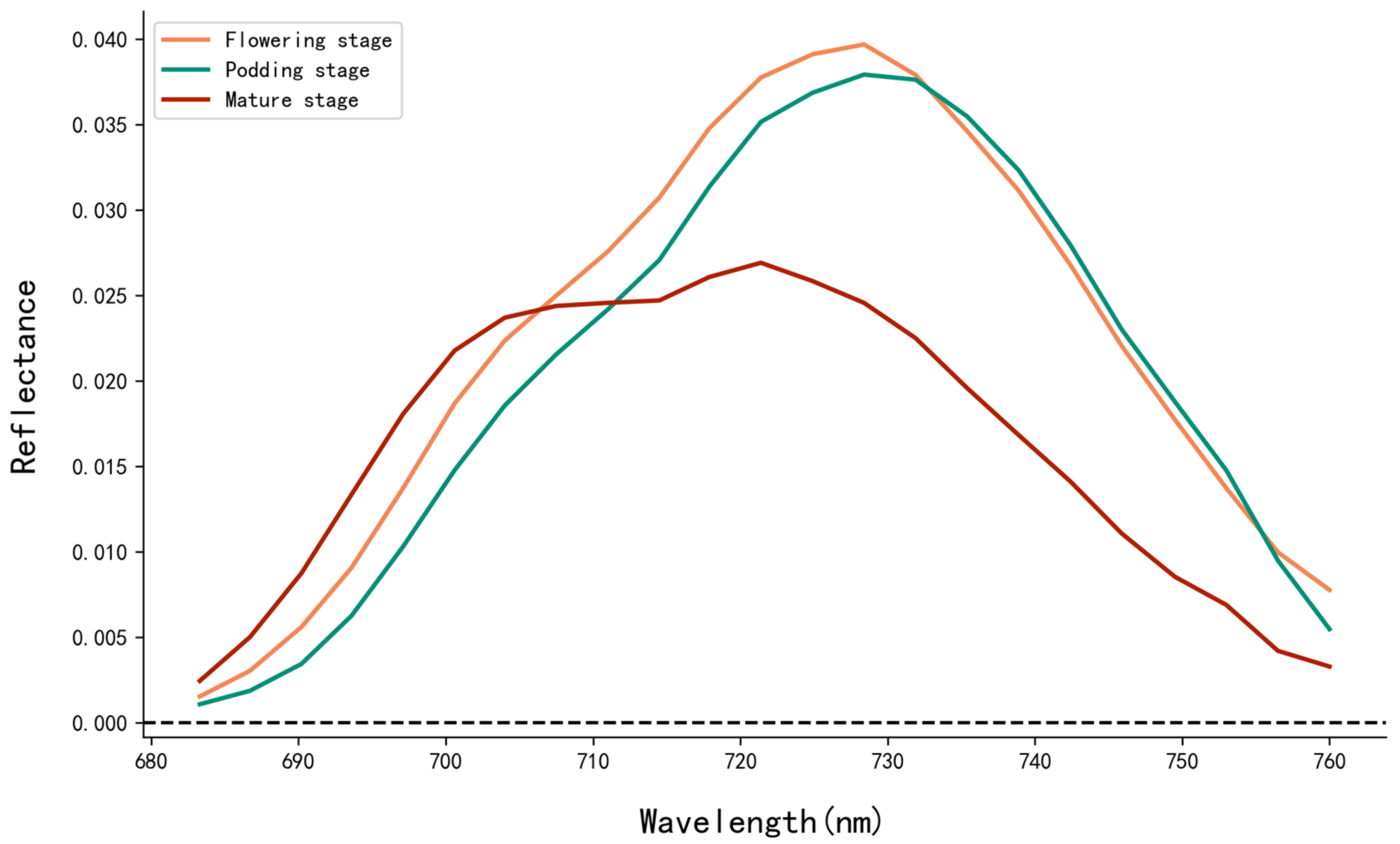
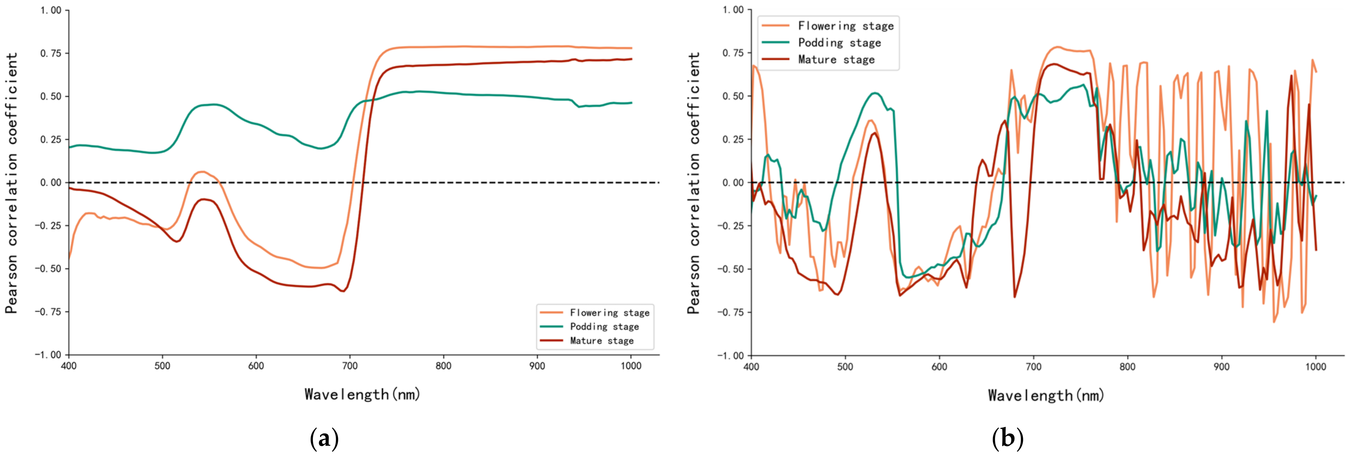
| Stage | Raw Spectral Reflectance Sensitive Band | Optimal Bands (nm) | First Derivative Reflectance Sensitive Band | Optimal Bands (nm) | Red Edge Amplitude | Red Edge Area |
|---|---|---|---|---|---|---|
| Flowering | 0.791 | 933 | −0.806 | 955 | 0.781 | 0.788 |
| Podding | 0.529 | 774 | 0.565 | 753 | 0.487 | 0.536 |
| Mature | 0.717 | 1000 | 0.685 | 721 | 0.672 | 0.673 |
| 1 Prediction Models | Flowering Stage | Podding Stage | Mature Stage | ||||
|---|---|---|---|---|---|---|---|
| R2 | RMSE | R2 | RMSE | R2 | RMSE | ||
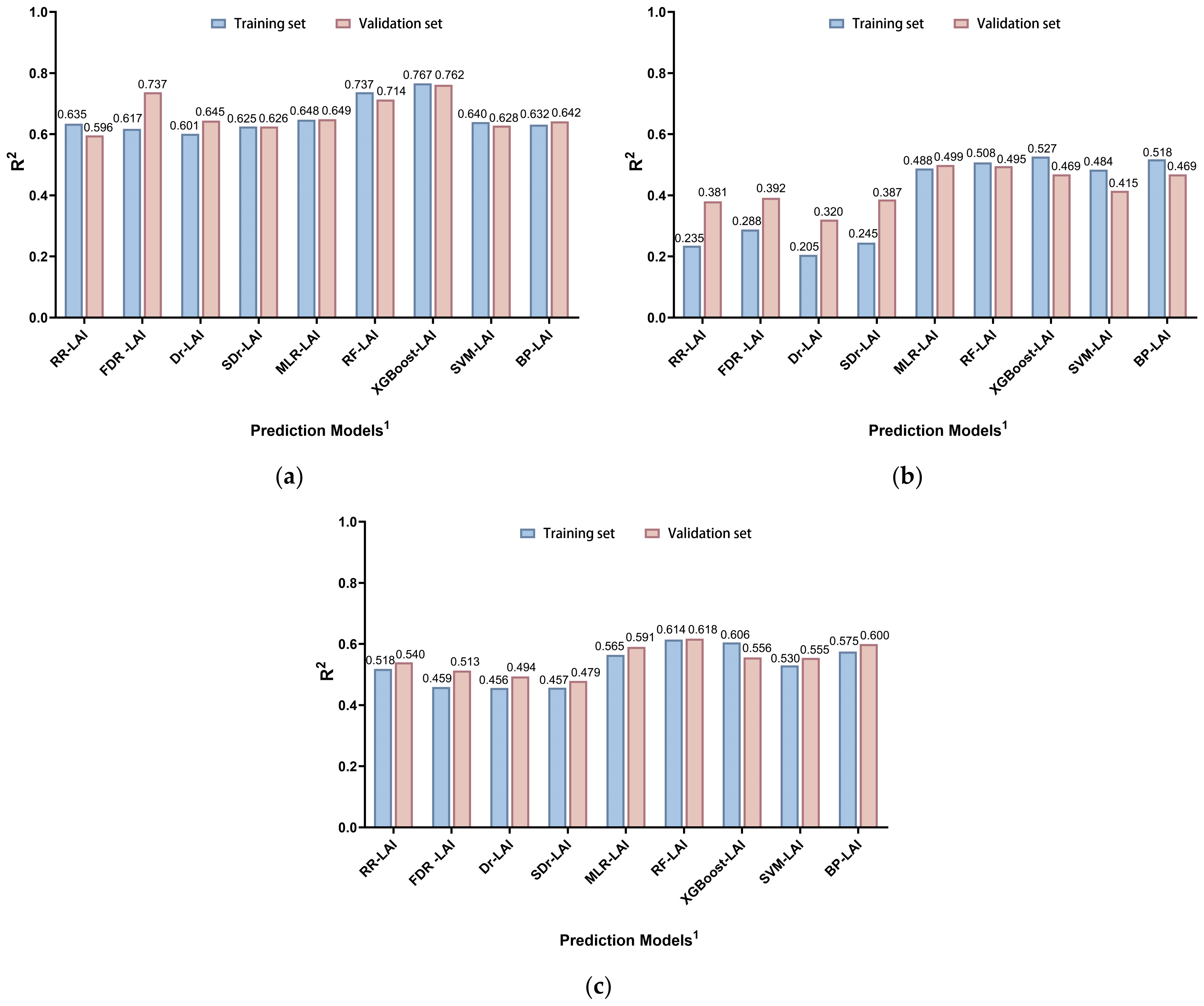
| RR-LAI | Training set | 0.635 | 0.349 | 0.235 | 0.401 | 0.518 | 0.373 |
| Validation set | 0.596 | 0.296 | 0.381 | 0.324 | 0.540 | 0.263 | |
| FDR-LAI | Training set | 0.617 | 0.352 | 0.288 | 0.428 | 0.459 | 0.372 |
| Validation set | 0.737 | 0.266 | 0.392 | 0.342 | 0.513 | 0.320 | |
| Dr-LAI | Training set | 0.601 | 0.355 | 0.205 | 0.382 | 0.456 | 0.372 |
| Validation set | 0.645 | 0.253 | 0.320 | 0.290 | 0.494 | 0.277 | |
| SDr-LAI | Training set | 0.625 | 0.351 | 0.245 | 0.407 | 0.457 | 0.372 |
| Validation set | 0.626 | 0.248 | 0.387 | 0.322 | 0.479 | 0.297 | |
| 1 Prediction Models | Flowering Stage | Podding Stage | Mature Stage | ||||
|---|---|---|---|---|---|---|---|
| R2 | RMSE | R2 | RMSE | R2 | RMSE | ||
| MLR-LAI | Training set | 0.648 | 0.346 | 0.488 | 0.473 | 0.565 | 0.370 |
| Validation set | 0.649 | 0.253 | 0.499 | 0.470 | 0.591 | 0.302 | |
| RF-LAI | Training set | 0.737 | 0.288 | 0.508 | 0.339 | 0.614 | 0.345 |
| Validation set | 0.714 | 0.277 | 0.495 | 0.303 | 0.618 | 0.240 | |
| XGBoost-LAI | Training set | 0.767 | 0.235 | 0.527 | 0.321 | 0.606 | 0.375 |
| Validation set | 0.762 | 0.236 | 0.469 | 0.305 | 0.556 | 0.338 | |
| SVM-LAI | Training set | 0.640 | 0.340 | 0.484 | 0.433 | 0.530 | 0.363 |
| Validation set | 0.628 | 0.264 | 0.415 | 0.379 | 0.555 | 0.264 | |
| BP-LAI | Training set | 0.632 | 0.308 | 0.518 | 0.450 | 0.575 | 0.360 |
| Validation set | 0.642 | 0.223 | 0.469 | 0.467 | 0.600 | 0.288 | |
| Prediction Models | R2 | RMSE | |
|---|---|---|---|
| MLR-LAI | Training set | 0.516 | 0.518 |
| Validation set | 0.486 | 0.431 | |
| RF-LAI | Training set | 0.738 | 0.391 |
| Validation set | 0.661 | 0.362 | |
| XGBoost-LAI | Training set | 0.737 | 0.391 |
| Validation set | 0.681 | 0.366 | |
| SVM-LAI | Training set | 0.581 | 0.509 |
| Validation set | 0.585 | 0.488 | |
| BP-LAI | Training set | 0.637 | 0.500 |
| Validation set | 0.691 | 0.423 | |
| Stages | LCI | NDRE | NDVI | GNDVI | OSAVI |
|---|---|---|---|---|---|
| Flowering | 0.654 | 0.637 | 0.670 | 0.669 | 0.754 |
| Mature | 0.540 | 0.501 | 0.659 | 0.627 | 0.688 |
| VIs | Flowering Stage | Mature Stage | |||
|---|---|---|---|---|---|
| R2 | RMSE | R2 | RMSE | ||
| LCI | Training set | 0.336 | 0.285 | 0.304 | 0.331 |
| Validation set | 0.601 | 0.309 | 0.260 | 0.253 | |
| NDRE | Training set | 0.304 | 0.277 | 0.263 | 0.317 |
| Validation set | 0.590 | 0.296 | 0.219 | 0.243 | |
| NDVI | Training set | 0.462 | 0.301 | 0.479 | 0.360 |
| Validation set | 0.559 | 0.464 | 0.389 | 0.291 | |
| GNDVI | Training set | 0.367 | 0.290 | 0.417 | 0.355 |
| Validation set | 0.623 | 0.346 | 0.370 | 0.267 | |
| OSAVI | Training set | 0.603 | 0.295 | 0.504 | 0.360 |
| Validation set | 0.596 | 0.455 | 0.462 | 0.299 | |
| Prediction Models | Flowering Stage | Mature Stage | |||
|---|---|---|---|---|---|
| R2 | RMSE | R2 | RMSE | ||
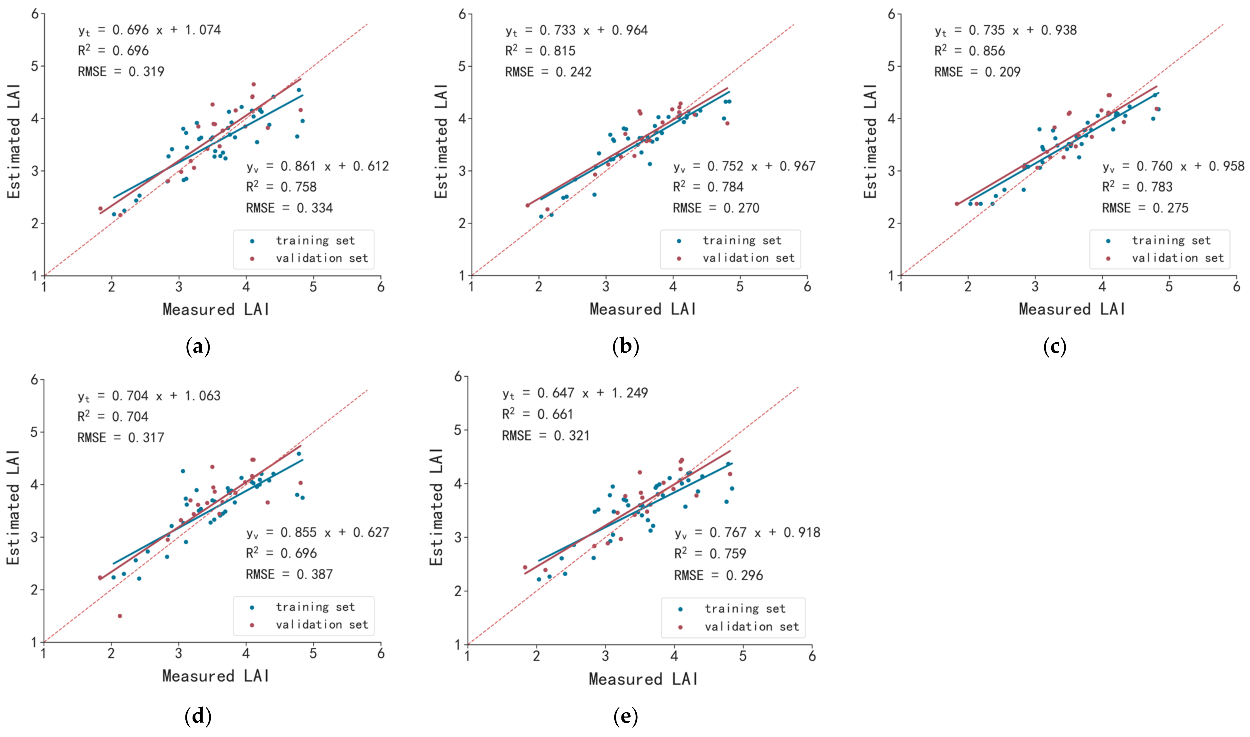
| MLR-LAI | Training set | 0.704 | 0.275 | 0.538 | 0.359 |
| Validation set | 0.649 | 0.337 | 0.539 | 0.297 | |
| RF-LAI | Training set | 0.739 | 0.241 | 0.564 | 0.249 |
| Validation set | 0.643 | 0.363 | 0.431 | 0.251 | |
| XGBoost-LAI | Training set | 0.749 | 0.206 | 0.582 | 0.301 |
| Validation set | 0.662 | 0.316 | 0.487 | 0.277 | |
| SVM-LAI | Training set | 0.678 | 0.335 | 0.608 | 0.339 |
| Validation set | 0.652 | 0.474 | 0.568 | 0.315 | |
| BP-LAI | Training set | 0.698 | 0.275 | 0.565 | 0.359 |
| Validation set | 0.656 | 0.389 | 0.623 | 0.253 | |
| LiDAR Parameters | Flowering Stage | LiDAR Parameters | Mature Stage | ||||
|---|---|---|---|---|---|---|---|
| R2 | RMSE | R2 | RMSE | ||||
| P75–100 | Training set | 0.414 | 0.320 | H50 | Training set | 0.188 | 0.271 |
| Validation set | 0.656 | 0.215 | Validation set | 0.228 | 0.235 | ||
| PAPCH | Training set | 0.319 | 0.302 | P50–100 | Training set | 0.142 | 0.242 |
| Validation set | 0.721 | 0.175 | Validation set | 0.342 | 0.190 | ||
| P50–100 | Training set | 0.400 | 0.318 | H75 | Training set | 0.197 | 0.276 |
| Validation set | 0.519 | 0.236 | Validation set | 0.201 | 0.232 | ||
| PCHmean | Training set | 0.256 | 0.283 | Hmean | Training set | 0.186 | 0.270 |
| Validation set | 0.642 | 0.159 | Validation set | 0.227 | 0.218 | ||
| P25–50 | Training set | 0.365 | 0.313 | PCHmean | Training set | 0.155 | 0.251 |
| Validation set | 0.628 | 0.212 | Validation set | 0.289 | 0.180 | ||
| Prediction Models | Flowering Stage | Mature Stage | |||
|---|---|---|---|---|---|
| R2 | RMSE | R2 | RMSE | ||
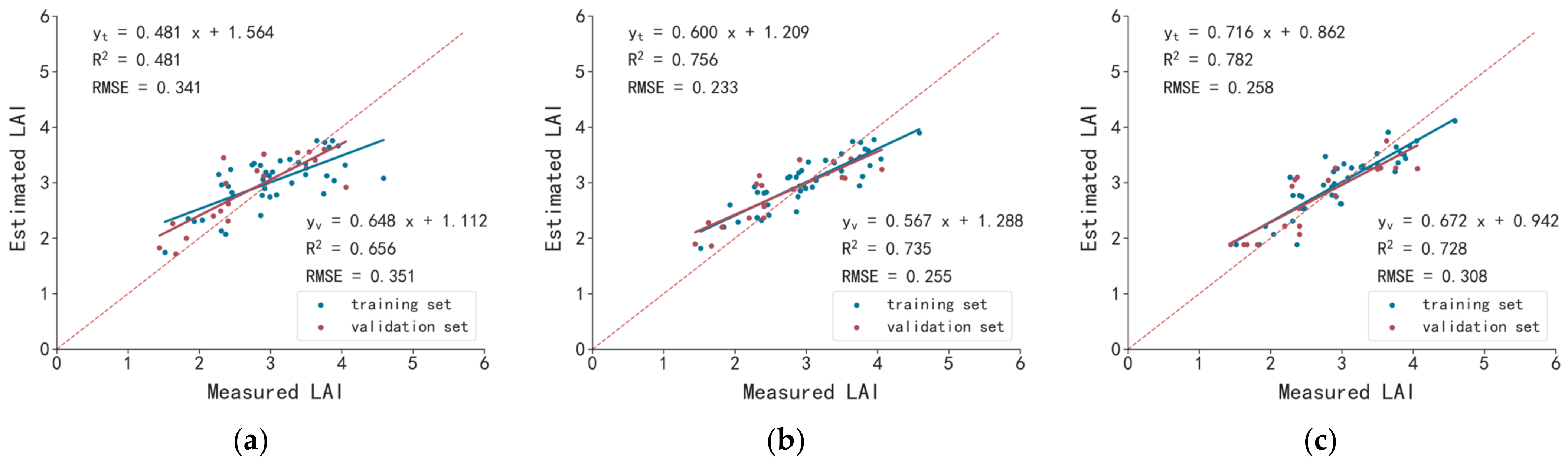
| MLR-LAI | Training set | 0.504 | 0.325 | 0.227 | 0.290 |
| Validation set | 0.551 | 0.250 | 0.227 | 0.243 | |
| RF-LAI | Training set | 0.710 | 0.261 | 0.411 | 0.215 |
| Validation set | 0.679 | 0.192 | 0.251 | 0.156 | |
| XGBoost-LAI | Training set | 0.647 | 0.282 | 0.297 | 0.196 |
| Validation set | 0.602 | 0.281 | 0.291 | 0.154 | |
| SVM-LAI | Training set | 0.568 | 0.323 | 0.275 | 0.301 |
| Validation set | 0.537 | 0.286 | 0.263 | 0.231 | |
| BP-LAI | Training set | 0.561 | 0.318 | 0.241 | 0.264 |
| Validation set | 0.579 | 0.226 | 0.270 | 0.201 | |
| Prediction Models | Flowering Stage | Mature Stage | |||
|---|---|---|---|---|---|
| R2 | RMSE | R2 | RMSE | ||
| MLR-LAI | Training set | 0.689 | 0.302 | 0.558 | 0.339 |
| Validation set | 0.720 | 0.388 | 0.572 | 0.489 | |
| RF-LAI | Training set | 0.754 | 0.235 | 0.673 | 0.223 |
| Validation set | 0.739 | 0.287 | 0.666 | 0.268 | |
| XGBoost-LAI | Training set | 0.752 | 0.260 | 0.647 | 0.290 |
| Validation set | 0.725 | 0.292 | 0.621 | 0.334 | |
| SVM-LAI | Training set | 0.692 | 0.293 | 0.645 | 0.308 |
| Validation set | 0.650 | 0.307 | 0.636 | 0.406 | |
| BP-LAI | Training set | 0.718 | 0.279 | 0.607 | 0.325 |
| Validation set | 0.692 | 0.344 | 0.624 | 0.372 | |
Disclaimer/Publisher’s Note: The statements, opinions and data contained in all publications are solely those of the individual author(s) and contributor(s) and not of MDPI and/or the editor(s). MDPI and/or the editor(s) disclaim responsibility for any injury to people or property resulting from any ideas, methods, instructions or products referred to in the content. |
© 2022 by the authors. Licensee MDPI, Basel, Switzerland. This article is an open access article distributed under the terms and conditions of the Creative Commons Attribution (CC BY) license (https://creativecommons.org/licenses/by/4.0/).
Share and Cite
Zhang, Y.; Yang, Y.; Zhang, Q.; Duan, R.; Liu, J.; Qin, Y.; Wang, X. Toward Multi-Stage Phenotyping of Soybean with Multimodal UAV Sensor Data: A Comparison of Machine Learning Approaches for Leaf Area Index Estimation. Remote Sens. 2023, 15, 7. https://doi.org/10.3390/rs15010007
Zhang Y, Yang Y, Zhang Q, Duan R, Liu J, Qin Y, Wang X. Toward Multi-Stage Phenotyping of Soybean with Multimodal UAV Sensor Data: A Comparison of Machine Learning Approaches for Leaf Area Index Estimation. Remote Sensing. 2023; 15(1):7. https://doi.org/10.3390/rs15010007
Chicago/Turabian StyleZhang, Yi, Yizhe Yang, Qinwei Zhang, Runqing Duan, Junqi Liu, Yuchu Qin, and Xianzhi Wang. 2023. "Toward Multi-Stage Phenotyping of Soybean with Multimodal UAV Sensor Data: A Comparison of Machine Learning Approaches for Leaf Area Index Estimation" Remote Sensing 15, no. 1: 7. https://doi.org/10.3390/rs15010007