Article

A Full Tensor Decomposition Network for Crop Classification with Polarization Extension

1
School of Electronic Engineering, Xidian University, Xi’an 710071, China
2
Research Institute of Advanced Remote Sensing Technology, Xidian University, Xi’an 710071, China
3
College of Mechanical and Electronic Engineering, Northwest A & F University, Xianyang 712100, China
4
Shanghai Institude of Satellite Engineering, Shanghai 201100, China
*
Author to whom correspondence should be addressed.
Remote Sens. 2023, 15(1), 56; https://doi.org/10.3390/rs15010056
Submission received: 29 October 2022 / Revised: 16 December 2022 / Accepted: 16 December 2022 / Published: 22 December 2022
(This article belongs to the Special Issue Deep Learning for Remote Sensing Image Classification II)

Abstract

:
The multisource data fusion technique has been proven to perform better in crop classification. However, traditional fusion methods simply stack the original source data and their corresponding features, which can be only regarded as a superficial fusion method rather than deep fusion. This paper proposes a pixel-level fusion method for multispectral data and dual polarimetric synthetic aperture radar (PolSAR) data based on the polarization extension, which yields synthetic quad PolSAR data. Then we can generate high-dimensional features by means of various polarization decomposition schemes. High-dimensional features usually cause the curse of the dimensionality problem. To overcome this drawback in crop classification using the end-to-end network, we propose a simple network, namely the full tensor decomposition network (FTDN), where the feature extraction in the hidden layer is accomplished by tensor transformation. The number of parameters of the FTDN is considerably fewer than that of traditional neural networks. Moreover, the FTDN admits higher classification accuracy by making full use of structural information of PolSAR data. The experimental results demonstrate the effectiveness of the fusion method and the FTDN model.

Graphical Abstract

1. Introduction

Crop classification plays an important role in the remote sensing monitoring of agricultural conditions. It is also a premise for further monitoring of crop growth and yields. Accurate and reliable discrimination of crop categories based on remotely-sensed images is a significant data source for agricultural monitoring and food security evaluation research.
Optical and radar remote sensing technologies are the two main methodologies for crop classification. Optical remote sensing technology is susceptible to environmental factors, such as weather and light, and is unable to obtain accurate surface information under adverse weather [1]. Radar remote sensing technology is insensitive to weather and light. Hence, the fusion of optical data and synthetic aperture radar (SAR) data is commonly carried out to implement more accurate classifications of crops [2]. For example, Qiao et al. fused SAR data and optical data and adopted a maximum likelihood method for crop classification based on fused data, leading to improved classification accuracy [3]. Shi et al. classified the fused data of multispectral and hyperspectral data through classification and regression tree, showing that the classification accuracies of fused data are better than those of individual data alone [4]. However, these fusion methods simply stack the multisource data or their corresponding features, they are far from in-depth fusion. Seo constructed a fusion model of optical data and SAR data using the random forest regression method, benefiting from the subsequent image analysis and interpretation [5]. This method fused the multisource data in-depth, which enhanced the quality of the optical image with auxiliary SAR data, and provided a new illustration for image fusion. Different from image fusion, the crop classification task focuses on the effective extraction of distinguishable features from remotely sensed data and the subsequent powerful classification model trained by these features. In particular, under the adverse weather condition, multisource data fusion is beneficial to generate enough distinguishable features for crop classification. In order to overcome the adverse weather effect, more polarization scattering features are always superior [6]. Quad PolSAR data usually provide data rich enough for crop classification, as it enables extracting large numbers of polarization scattering features via various polarization decomposition schemes [7]. However, quad PolSAR data are usually unavailable due to their higher costs. Dual PolSAR data can be served as natural substitutes, but fewer polarization decomposition schemes can be adopted, providing inadequate polarization scattering features. Therefore, the extension of dual PolSAR data to quad PolSAR data with the assistance of optical data is promising for crop classification.
Although higher dimensional features usually improve crop classification performance, it is prone to result in the “curse of dimensionality” problem in real applications. As for a regular cognitive model, the higher dimensional features extracted from raw data contain more information, and the trained model will be more capable to deal with sophisticated issues. However, Hughes [8] shows that the prediction ability of the model is enhanced at the beginning and then deteriorated with the increase of feature dimension for a fixed number of learning samples. This is called the Hughes phenomenon, which is one of the most significant drawbacks caused by the “curse of dimensionality”. This eventually results in a contradiction between the feature space and sample space below. To solve this problem, dimensionality reduction methods, including Principal Component Analysis (PCA) [9], Locally Linear Embedding (LLE) [10], and Autoencoder [11], are generally adopted before classification. Moreover, the subsequent classifiers, such as support vector machine (SVM) [12], K-nearest neighbor (KNN) [13] and neural networks [14,15,16] worked on the compressed features. However, these two-stage methods destroyed the structural information of high-dimensional data, and the hard connection between the dimensionality reduction model and classification model usually leads to a degraded performance. Fortunately, tensor decomposition techniques, such as Tucker decomposition and CP decomposition [17], are efficient tool to extract features from higher dimensional data with fewer parameters [18]. Moreover, it preserves the structural information in the decomposed core tensor. These two merits make it suitable to serve as the feature extractor or data compressor in higher dimensional scenario. However, tensor decomposition always works in an offline mode, where the transformation parameters such as the loading matrices depend only on the individual tensor sample. They cannot be properly learned online by a set of data samples. Therefore, the tensor decomposition-based learning method is promising to incorporate compressor and classifier in an end-to-end network.
In order to solve the above problems, we propose a polarization extension method for multisource data fusion and a full tensor decomposition network (FTDN) for end-to-end crop classification. The polarization extension method extends dual PolSAR to synthetic quad PolSAR data, then providing more complementary polarization scattering features to optical data. The FTDN is a one-stage network with fewer parameters, which exploits tensor decomposition technique in each layer to implement feature extraction and pattern classification. It is able to extract structural information from the original high-dimensional data, and circumvent the curse of dimensionality through tensor decomposition.
The rest of the paper is organized as follows. The second part presents the polarization extension-based fusion method, feature collection themes, and the architecture of the FTDN. The third part provides experimental results to verify the feasibility of the proposed method. The fourth part discusses the experimental results. Finally, our conclusion is drawn in Section 5.

2. Proposed Methodology

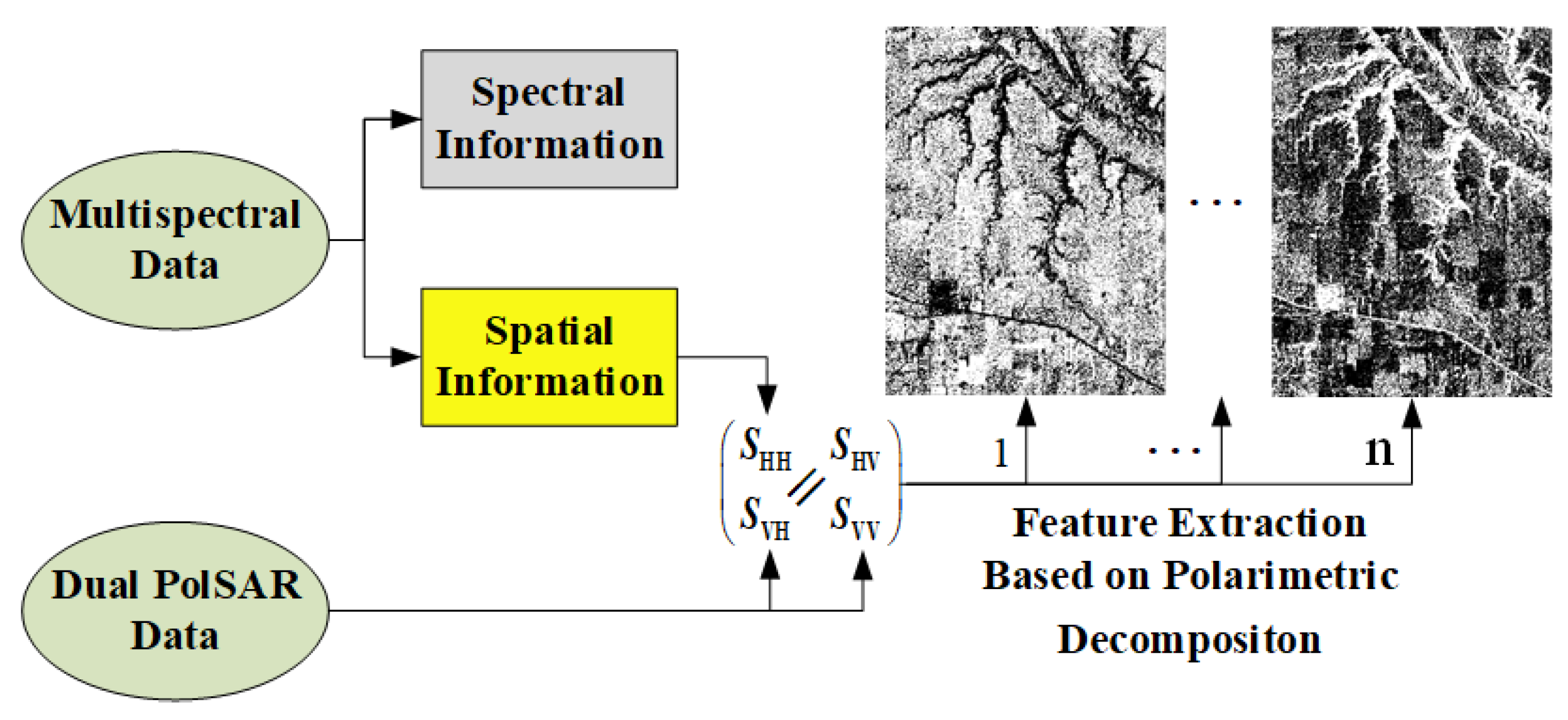
2.1. Multisource Data Fusion via Polarization Extension

Multispectral data and SAR data provide complementary features. The fusion of SAR data and multispectral data contributes to the better visual perception of objects and compensates for spatial information. Intensity hue saturation (IHS) and PCA methods are often used to merge multisensor data [19]. Chavez investigated the feasibility of three methods for using panchromatic data to substitute spatial features of multispectral data (both statistically and visually) [20]; Chandrakanth demonstrated the feasibility of the fusion of SAR data and multispectral data [21]. A basic assumption concerning these methods is that the SAR amplitude is closely related to the intensity and principal component of multispectral images with high correlation coefficients. Therefore, SAR data can replace either of these two images while re-transforming data back into the original image space. Inspired by this assumption, we propose to consider an antithetical assumption that the principal component of multispectral images can be regarded as PolSAR data from the point of view of intensity, which yields the simulated SAR data in a certain polarization mode. Then the dual PolSAR data can be extended to construct synthetic quad PolSAR data.
For quad PolSAR data, each pixel is represented by a 2 × 2 complex matrix as follows
S = S H H S H V S V H S V V
where S H V denotes the scattering factor of horizontal transmitting and vertical receiving polarization and the others have similar definitions. Here we demonstrate the fusion of multispectral data and dual PolSAR data generated in VH and VV polarization modes. Note that the reciprocity condition S H V = S V H is commonly assumed for quad PolSAR data, then we only need to construct the scattering factor S H H 
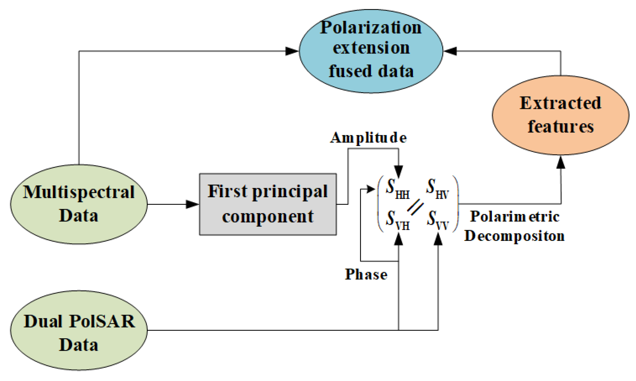
to form the quad PolSAR data. Firstly, we perform the registration of imageries collected by different sensors in advance. The overall fusion process is then illustrated in Figure 1. On one hand, we extract the principal component of multispectral data using PCA. The extracted principal component represents the spatial information, which is used to generate the amplitude of S H H . On the other hand, the phase of S H H is simulated by using the phase of S H V instead. This is because they shared the same horizontal polarization transmitting antenna. Moreover, most of the distinguishable features (see Table 1 below) for crop classification is irrelevant to the phase of scattering factor, and our experimental results show that the crop classification performance is insensitive to the phase of S H H . Finally, the simulated S H H is incorporated into the dual polarization data S V H and S V V to form synthetic quad PolSAR data, which enables us to extract higher dimensional features of the target through various polarimetric decomposition schemes. High-dimensional features extracted from synthetic quad PolSAR data provide more complementary information to multispectral data for accurate classification applications.

2.2. Polarization Decomposition and Feature Collection

Polarization scattering feature extraction of PolSAR data can obtain more target feature information and further improve the classification, detection, and identification capabilities of a data-driven model. A quad PolSAR image can obtain the 36-dimensional polarimetric scattering features by using a variety of classical decomposition algorithms. As shown in Table 1, 10 features were directly obtained from the measured data by simple transformations and combinations. We obtained 24 features using incoherent decomposition algorithms, including the Huynen decomposition [22], Freeman–Durden decomposition [23], Yamaguchi decomposition [24], and Cloude–Pottier decomposition [25]. The last 2 null angle parameters were computed via polarimetric matrix rotation [26]. A quad PolSAR image was processed and the 36-dimensional features were obtained. The resulting features involved all of the potential data of the primitive PolSAR data.

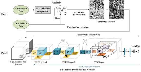
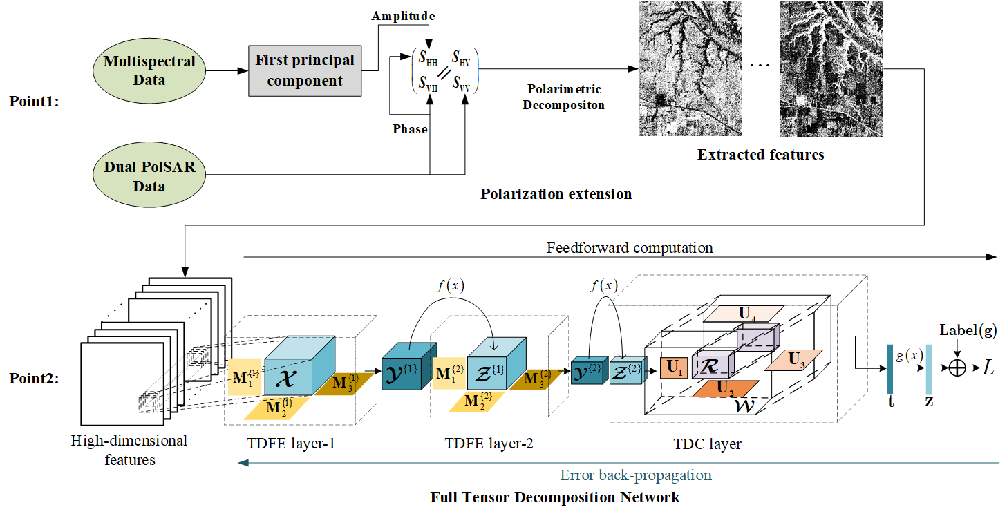
2.3. Full Tensor Decomposition Network

(1) Tucker decomposition-based feature extraction layer: When using the traditional neural network to classify high dimensional crop data, it is often necessary to perform dimensionality reduction operations to avoid the curse of dimensionality. Moreover, the extracted features from the data compressor may not be suitable for the classification model because the compressor and classification model are separately trained. We propose a Tucker decomposition-based feature extraction (TDFE) layer to extract hidden information from high-dimensional data. The TDFE layer can be used as the hidden layer of a tensor network, which performs the data compression or feature extraction for further processing.
The TDFE layer, different from the fully connected layer, uses tensor decomposition to realize the forward propagation. For a 3-way tensor X = { x i 1 i 2 i 3 } R I 1 × I 2 × I 3 , a compressed feature tensor Z = { z j 1 j 2 j 3 } R J 1 × J 2 × J 3 can be obtained by transforming X as follows
Y = X × 1 M 1 × 2 M 2 × 3 M 3
Z = f ( Y )
where M n R J n × I n , n = 1 , 2 , 3 are factor matrices, × 1 performs the operation that multiplies each column fiber of X with M 1 , × 2 performs the operation that multiplies each row fiber of X with M 2 , and × 3 performs the operation that multiplies each tube fiber of X with M 3 , Y = { y j 1 j 2 j 3 } R J 1 × J 2 × J 3 is the multi-linear transformed tensor and f ( · ) is the activation function. Note that the outcome Y is independent of the calculation order of mode product, each component y j 1 j 2 j 3 in tensor Y is calculated by
y j 1 j 2 j 3 = i 1 = 1 I 1 i 2 = 1 I 2 i 3 = 1 I 3 x i 1 i 2 i 3 m 1 j 1 i 1 m 2 j 2 i 2 m 3 j 3 i 3
where m 1 j 1 i 1 , m 2 j 2 i 2 , m 3 j 3 i 3 are corresponding entries in matrices M 1 , M 2 and M 3 . The forward propagation of the TDFE layer can be regarded as the inverse process of Tucker decomposition. The TDFE layer allows us to decompose the input tensor without destroying its coupling structure between each mode.
The factor matrices M n are learned end-to-end by error backpropagation. When the TDFE layer is regarded as a hidden layer of a tensor neural network, we define the neuron error tensor E of the TDFE layer as E = Δ L Y = { e j 1 j 2 j 3 } R J 1 × J 2 × J 3 ,where L represents the loss function of the network. The update of each entry m 1 j 1 i 1 M 1 is derived by finding the gradient
L m 1 j 1 i 1 = j 2 = 1 J 2 j 3 = 1 J 3 L y j 1 j 2 j 3 y j 1 j 2 j 3 m 1 j 1 i 1 = j 2 = 1 J 2 j 3 = 1 J 3 i 2 = 1 I 2 i 3 = 1 I 3 e j 1 j 2 j 3 x i 1 i 2 i 3 m 2 j 2 i 2 m 3 j 3 i 3
The updates of M 2 and M 3 are similar to that of M 1 .
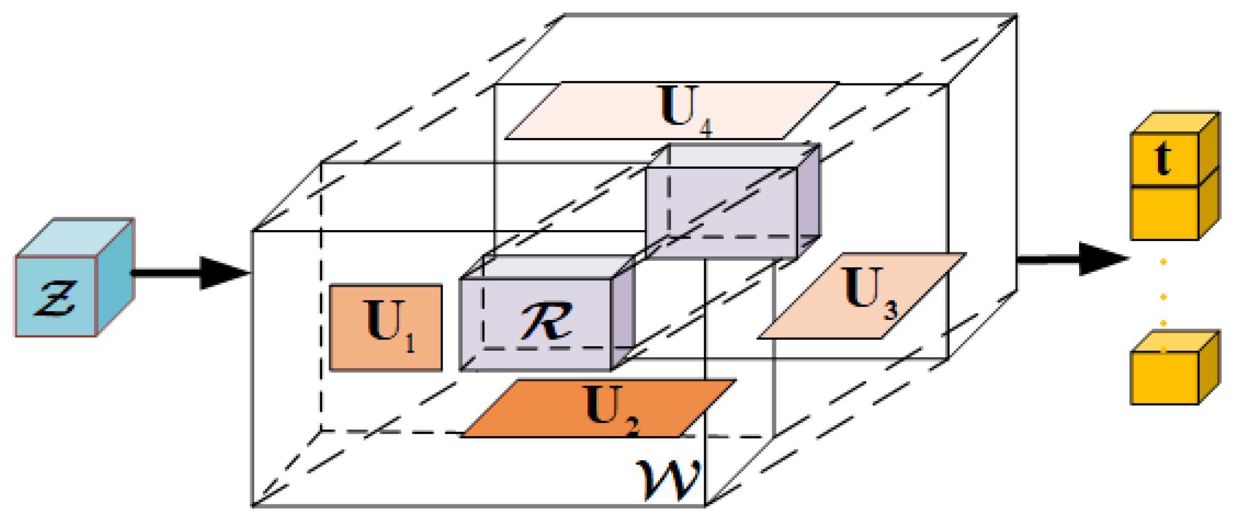
(2) Tucker decomposition-based classification layer: A flattened layer is always necessary for classical networks to vectorize the resulting features extracted by the hidden layer when classification or regression is performed. However, the structural information from the high-dimensional feature tensor will be discarded after the flattened layer. Instead, we propose to use a higher order weight tensor W to project the feature tensor into a class vector without discarding the multimodal structure. The higher order weight tensor W usually contains a large number of parameters, the update of which will lead to extremely high computational complexity. Here we proposed a Tucker decomposition-based classification (TDC) layer, which used the low-rank representation to replace the original weight tensor.
Figure 2 illustrates the structure of the TDC layer. Assuming that the 3-way feature tensor Z = { z k 1 k 2 k 3 } R K 1 × K 2 × K 3 is fed to the TDC layer, an output vector t = { t k 4 } R K 4 can be generated by a 4-way weight tensor W = { w k 1 k 2 k 3 k 4 } R K 1 × K 2 × K 3 × K 4 , where K 4 is the number of classes and each component t k 4 is calculated by the inner product of Z and the slices of W
t k 4 = Z , W k 4 = k 1 = 1 K 1 k 2 = 1 K 2 k 3 = 1 K 3 z k 1 k 2 k 3 w k 1 k 2 k 3 k 4
where denotes the inner product of two tensors, and W k 4 is the slice of W along the fourth way. In order to reduce the parameters of the TDC layer, the weight tensor W is decomposed and represented by a core tensor R R Q 1 × Q 2 × Q 3 × Q 4 and factor matrices U n R K n × Q n
W = R × 1 U 1 × 2 U 2 × 3 U 3 × 4 U 4
Then substituting (6) into (5) leads to
t k 4 = k 1 = 1 K 1 k 2 = 1 K 2 k 3 = 1 K 3 q 1 = 1 Q 1 q 2 = 1 Q 2 q 3 = 1 Q 3 q 4 = 1 Q 4 z k 1 k 2 k 3 r q 1 q 2 q 3 q 4 · u 1 k 1 q 1 u 2 k 2 q 2 u 3 k 3 q 3 u 4 k 4 q 4 = q 1 = 1 Q 1 q 2 = 1 Q 2 q 3 = 1 Q 3 ( k 1 = 1 K 1 k 2 = 1 K 2 k 3 = 1 K 3 z k 1 k 2 k 3 u 1 k 1 q 1 u 2 k 2 q 2 u 3 k 3 q 3 ) · ( q 4 = 1 Q 4 r q 1 q 2 q 3 q 4 u 4 k 4 q 4 ) = Z , R k 4
where Z and R k 4 are 3-way smaller tensors of dimension Q 1 × Q 2 × Q 3 , since Q n can be always chosen far less than K n . Note that the parameters of the TDC layer are converted to smaller core tensor R and the factor matrices U 1 , , U 4 . Therefore, the number of parameters of the network can be greatly reduced.
When the TDC layer is used as the classification layer of a tensor neural network, the parameters of the TDC layer are learned end-to-end by error backpropagation. Let us define the neuron error vector e of the TDC layer as e = Δ L t = { e k 4 } R K 4 , then the update of R and U 1 are derived by finding the gradient
L r q 1 q 2 q 3 q 4 = k 1 = 1 K 1 k 2 = 1 K 2 k 3 = 1 K 3 k 4 = 1 K 4 e k 4 z k 1 k 2 k 3 · u 1 k 1 q 1 u 2 k 2 q 2 u 3 k 3 q 3 u 4 k 4 q 4
L u 1 k 1 q 1 = k 2 = 1 K 2 k 3 = 1 K 3 k 4 = 1 K 4 e k 4 z k 1 k 2 k 3 q 2 = 1 Q 2 q 3 = 1 Q 3 q 4 = 1 Q 4 r q 1 q 2 q 3 q 4 u 2 k 2 q 2 u 3 k 3 q 3 u 4 k 4 q 4
The update of each entry U 2 , U 3 , and U 4 is similar to that of U 1 .
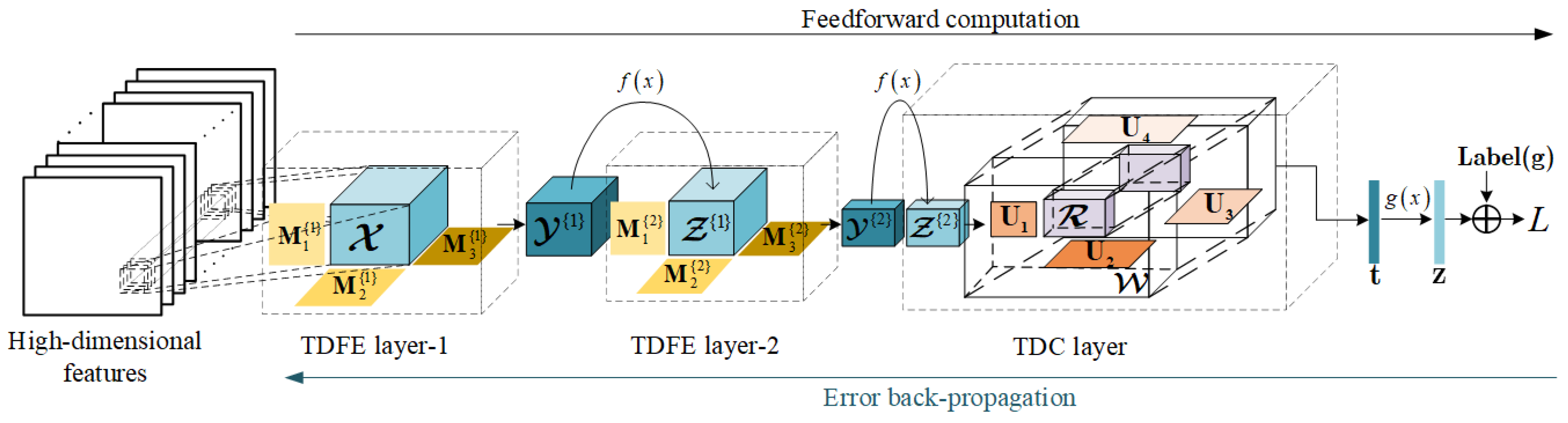
(3) FTDN architecture and learning: Based on TDFE layer and TDC layer, we propose a full tensor decomposition network (FTDN) for high-dimensional data classification. The architecture of the FTDN is shown in Figure 3, which contains two TDFE layers and one TDC layer. The input tensor sample X = { x i 1 i 2 i 3 } R I 1 × I 2 × I 3 that corresponds to a certain pixel is formed by collecting all features of its local neighborhood pixels, where I 3 is the number of features and I 1 × I 2 is the size of the neighborhood. For TDFE layer-1, the feedforward computation is straightforward, and its output feature tensor is denoted by Z { 1 } = { z j 1 j 2 j 3 { 1 } } R J 1 × J 2 × J 3 , where the superscript in the bracket denotes the layer index. For TDFE layer-2, the input tensor comes from the output of the previous layer, and the output feature tensor is denoted by Z { 2 } = { z k 1 k 2 k 3 { 2 } } R K 1 × K 2 × K 3 . For the TDC layer, the output vector t is transformed by a softmax layer to calculate the class posteriors z , where g ( x ) represents the softmax function.
We now derive the error backpropagation-based learning of the FTDN. We see that a stochastic gradient descent learning for the FTDN is straightforward according to Equation (3), (7) and (8), where the remained issue is to compute the neuron errors of each layer. As for layer TDC layer, the neuron error vector e depends on the specific loss function L, which can be chosen from typical cross-entropy or mean square error between the network output and target label. Taking the cross entropy loss, for example, the neuron error vector e reads e = z g , where g denotes the corresponding label vector. As for TDFE layer-2, the entries e k 1 k 2 k 3 { 2 } of neuron error tensor E { 2 } can be computed from e via the error backpropagation technique
e k 1 k 2 k 3 { 2 } = k 4 = 1 K 4 L t k 4 t k 4 z k 1 k 2 k 3 { 2 } z k 1 k 2 k 3 { 2 } y k 1 k 2 k 3 { 2 } = f y k 1 k 2 k 3 { 2 } k 4 = 1 K 4 e k 4 q 1 = 1 Q 1 q 2 = 1 Q 2 q 3 = 1 Q 3 q 4 = 1 Q 4 r q 1 q 2 q 3 q 4 u 1 k 1 q 1 u 2 k 2 q 2 u 3 k 3 q 3 u 4 k 4 q 4
Similarly, the error backpropagation from E { 2 } to E { 1 } is represented as
e j 1 j 2 j 3 { 1 } = k 1 = 1 K 1 k 2 = 1 K 2 k 3 = 1 K 3 L y k 1 k 2 k 3 { 2 } y k 1 k 2 k 3 { 2 } z j 1 j 2 j 3 { 1 } z j 1 j 2 j 3 { 1 } y j 1 j 2 j 3 { 1 } = f y j 1 j 2 j 3 { 1 } k 1 = 1 K 1 k 2 = 1 K 2 k 3 = 1 K 3 e k 1 k 2 k 3 { 2 } m 1 k 1 j 1 { 2 } · m 2 k 2 j 2 { 2 } m 3 k 3 j 3 { 2 }

3. Experimental Results

3.1. Experimental Data

(1) Dali Dataset: The study area in Dali dataset is a farm ( 109 10 49 E , 3 4 47 60 N ), located in Dali County, Weinan City, Shaanxi Province, which has 1106 × 514 pixels. There are mainly five different kinds of targets and an `unknown’ class in this area; the data are shown in Table 2, and the corresponding images of this area are shown in Figure 4.
As shown in Figure 4, the study area is covered by clouds. Five types of data are used in the following experiments: dual PolSAR data, multispectral data, stacking-based fusion data, textural feature fusion data, and polarization extension-fused data. The dual PolSAR data are obtained from the Sentinel-1 satellite with VV and VH polarization modes, and the multispectral data are obtained from the Sentinel-2 satellite. Stacking-based fusion data are formed by stacking multispectral data and original dual PolSAR data. In order to construct textural feature fusion data, we adopt gray-level co-occurrence matrix (GLCM) [27] method to extract textural features of dual PolSAR data, including energy, homogeneity and entropy. Then textural feature fusion data are obtained by combining the extracted features of VV and VH data respectively with multispectral data.
As for the polarization extension-fused data, the generation procedure is illustrated in Figure 5. Firstly, the principal component of the multispectral information is obtained by the standard PCA. Then we use the principal component to form the amplitude of S H H , and the phase of S H H is simulated by using the phase of S H V instead. Consequently, the synthetic HH channel data S H H and the dual PolSAR data are combined to obtain synthetic quad PolSAR data. Finally, the 36-dimensional features can be computed according to Table 1, and the combination of the extracted features with multispectral data yields the polarization extension-fused data.
(2) Flevoland Dataset:The Flevoland dataset was acquired by the NASA/JPL AIRSAR system in August 1989. This area has 15 classes of different types of crops and an `unknown’ class with 750 × 1024 pixels. The number of pixels and total area for each crop are summarized in Table 3. Figure 6a is the Pauli RGB image of the study area. The true distribution of crops is shown in Figure 6b [28,29]. As described in Section 2, the 36-dimensional features were collected for the Flevoland dataset, in the following experiments, we performed the model training and prediction based on the 36-dimensional features.

3.2. Classification Result of Different Methods Using Polarization Extension-Fused Data

We conducted an experiment on the Dali dataset to confirm the validity of the proposed method for crop classification. We compared FTDN with the state of art SAE-CNN [30], 3D CNN [31], classifiers, and other traditional deep learning methods [32] based on polarization extension-fused data to confirm the validity of the proposed methods.
For fair comparisons, the dimensions of the input data were reduced to 5 through the corresponding dimensionality reduction models for SAE-CNN and 3D CNN. For the FTDN, SAE-CNN, and 3D CNN classifiers, the sizes of the input samples were set to 5 × 5, while for other classifiers, the input single samples were without neighborhood pixels. The learning rate was set to 0.001 and the optimizer we adopted was adaptive moment estimation. for the FTDN, we used the activation function hyperbolic tangent for all TDFE layers. All methods were trained and implemented on our computing server equipped with two Intel Xeon E5-2620 CPUs and four Nvidia TITAN XP GPUs. Overall accuracy (OA) and Kappa coefficient (Kappa) were used to evaluate the classification accuracies of these methods. Each experiment repeated 10 times with randomly selected training samples.
The classification results of SAE-CNN, 3D CNN, 1D CNN, LSTM, and FTDN methods using polarization extension-fused data are shown in Figure 7. Table 4 presents a quantitative comparison of the classification accuracy and the number of parameters of the networks. Stratified random sampling was commonly implemented for accuracy assessment [33]; the training samples were selected using stratified random sampling with a 1% ratio.
We can conclude from Table 4 that the FTDN behaves the best performance. From the perspective of OA, the FTDN method is 2.17% higher than 3D CNN, 2.56% higher than SAE-CNN, 2.84% higher than 1D CNN, and 1.65% higher than LSTM. As for Kappa coefficient, the FTDN method is 4.12% higher than 3D CNN, 4.91% higher than SAE-CNN, 5.40% higher than 1D CNN and 2.34% higher than LSTM. Comparing the number of parameters of the networks, the FTDN is 89.14% fewer than 3D CNN, 94.73% fewer than SAE-CNN, 99.98% fewer than 1D CNN and 99.97% fewer than LSTM. These results indicate that classification using polarization extension-fused data achieves excellent effects, and the FTDN method has the best classification accuracy.
It should be pointed out that the proposed FTDN, 1D CNN, and LSTM are single end-to-end models for crop classification free of the specialized dimensionality compression model. The FTDN allows us to extract features without destroying its coupling structure between each mode, then the extracted structural information yields better classification accuracy. The fewer network parameters demonstrate the reason why FTDN can circumvent the curse of dimensionality [29]. However, for 3D CNN and SAE-CNN methods, the hard coupling between the feature compression model and the classification model is inevitable. After dimensionality reduction by data compression model, the input features are not necessarily discriminative for the classifier. As for 1D CNN and LSTM methods, although these classifiers maintain the end-to-end structure, these classifiers are usually used to process sequence data. The features of polarization extension-fused data contain few continuous sequence features and the characteristics of their network architectures determine that these classifiers cannot extract sufficient information for classification. The FTDN is a single end-to-end model for crop classification without hard coupling, and the special multi-way feature extraction technique based on the Tucker decomposition along each mode is efficient at capturing the structural distinctions between different crops. These results demonstrate the superiority of the FTDN method.

3.3. Classification Result of Different Methods Using the Flevoland Dataset

In the previous experiment, the FTDN method is used for the first time to classify polarization extension data, the results validate its superiority. However, Dali dataset is a relatively simple dataset with only five different categories, which cannot demonstrate the classification capability sufficiently. In order to investigate the performance of the FTDN method in high-dimensional crop classification from multiple aspects, we present the experimental results on Flevoland dataset.
The classification results and error maps for the SVM, SAE-CNN, 3D CNN, 1D CNN, LSTM, vision transformer (ViT) [34], and FTDN methods are shown in Figure 8. It is noticeable that the FTDN behaves the best performance.
By further summarizing the recall rates of crops of 15 categories individually in Table 5, we can see that the recall rates of the FTDN for each category are universally higher than that of other methods. It is noticeable that the training samples are randomly selected with a 1% ratio for each category. Although the training sample numbers between different categories are unbalanced, the statistical distribution of the training samples was consistent with the distribution of the overall samples, the classification results will obey the prior distribution of crops. Extra experiments were also carried out, the results show that the overall accuracies under balanced samples case and unbalanced case are close to each other. In particular, for some categories with small planting areas, i.e., C1, C10, C12, and C15, the FTDN still yields excellent classification performances. The recall rates of other classifiers for these crops are poorer than the FTDN. Note that this corresponds to a small-sample learning problem; the results imply that the proposed FTDN is qualified for the small-sample learning problem to some extent. The low overall accuracy of other classifiers arises from the poorer classification performance for small planting areas. We believe that large scale networks, such as SAE-CNN and ViT, are not suitable for handling the small-sample learning scenario because the small samples are not adequate to train the large parameter amounts. The FTDN model is a simple network with only two TDFE layers and one TDC layer, which makes it more suitable for the small-sample learning problem. Therefore, the classification accuracy of small sample crops can be improved.
The number of parameters for a crop classification model is also very important because it affects the efficiency of the model implemented in a specified platform. The number of parameters of the FTDN, ViT, LSTM, 1D CNN, 3D CNN, and SAE-CNN are shown in Table 6. It can be observed that the total number of parameters for the FTDN is fewer than that of 3D CNN, SAE-CNN, 1D CNN, LSTM, and ViT. The sizes of the factor matrices determine the number of parameters of the FTDN, which are far less than convolution kernels. The FTDN can circumvent the increasing parameters caused by high-dimensional input data, which is why the FTDN can integrate the dimensionality reduction model and the classification model in a single network. The fewer parameters imply that the FTDN model is more suitable to efficiently be implemented in resource-limited-embedded platforms.

4. Discussion

4.1. Classification Results of the SVM Using Different Datasets

We can conclude from Section 3 that all classifiers achieved excellent classification accuracies using polarization extension-fused data. In order to further explore the superiorities of the polarization extension method, we used the SVM classifier here to classify different types of fusion data and compare the classification results.
The classification results of the five different datasets using the SVM method are shown in Figure 9, Table 7 presents a quantitative comparison of the classification accuracy. Training samples were randomly selected with 1% ratio, and the remaining samples were used for the test. The regularization parameter for the SVM was set to 0.8.
We can conclude from Table 7 that the OA of the SVM method, which used the polarization extension-fused data, was 1.92% higher than the textural feature fusion data, 5.65% higher than the stacking-based fusion data, 5.75% higher than multispectral data, and 20.5% higher than dual PolSAR data. The Kappas of the SVM method that used the polarization extension-fused data were 3.67% higher than textural feature fusion data, 12.34% higher than stacking-based fusion data, 12.58% higher than multispectral data, and 24.98% higher than dual PolSAR data.
Since the study area is covered by clouds, it is difficult to achieve outstanding accuracy by directly classifying multispectral data using the SVM method. Furthermore, the dual PolSAR data provide few features, they are insufficient for the SVM classifier to yield good classification performance. Simply stacking dual PolSAR data and multispectral data cannot take full use of the complementary advantages of multisource data, which only provide few accuracy improvements for crop classification. Textural features are more distinguishable for the classifier than the original dual PolSAR data, and fusing these features with multispectral data can improve classification accuracy. Therefore, the classification accuracies of textural feature fusion data outperform stacking-based fusion data. The proposed polarization extension method extracted higher dimensional radar features by generating synthetic quad PolSAR data, which provided more complementary data to multispectral data. The spatial data of multispectral data were very similar to SAR data, and could be regarded as good alternates to a certain polarization channel for PolSAR data. Hence, the synthetic quad PolSAR data can be used to approximate the real quad PolSAR data. We can obtain the 36-dimensional features from synthetic quad PolSAR data by various polarization decomposition schemes; the extracted 36-dimensional features are more distinguishable than textural features extracted by the GLCM from dual PolSAR data. Therefore, the classification accuracies of the polarization extension-fused data outperformed textural feature fusion data.

4.2. Performance of the FTDN on Different Tensor Samples and Train Ratios

We tested the FTDN classification performance and compared it with the SAE-CNN network and 3D CNN network under different input sizes. It should be noted that the 36-dimensional features are directly fed to the proposed FTDN, whereas the dimensions of the input features are reduced to 9 through corresponding dimensionality reduction models for SAE-CNN and 3D CNN. Table 8 shows the OA and Kappa coefficients of these classifiers with different input sizes under the 1% train ratio.
By observing Table 8, we conclude that these classifiers trained by larger input sizes perform better than smaller ones. The FTDN classifier can achieve superior classification accuracy under various input sizes; however, other classifiers are susceptible to the input sizes. In particular, the OA of the FTDN classifier is 5.37% higher than that of SAE-CNN and 5.30% higher than that of 3D CNN when the input size is set to 3 × 3, and 4.61% higher than that of SAE-CNN and 4.92% higher than that of 3D CNN when the input size is set to 7 × 7. The gap of OA (of different classifiers) will diminish as the input size increases. As for various input sizes, the classification performance of the FTDN is always better than SAE-CNN and 3D CNN. The excellent performance of the FTDN arises from the special multi-way feature extraction technique that is based on the TDFE layers, which can capture the structural distinctions in smaller tensor samples. However, the corresponding network architectures of 3D CNN and SAE-CNN cannot perform better in feature extracting when inputting smaller sample sizes. The input size 15 × 15 achieved excellent performance for all classifiers; therefore, there is no need to further increase the sizes of the input tensors because the computational burden increases accordingly. So, in the following experiments, we set the input sizes of these classifiers to 15 × 15.
The classification accuracy of different methods can be improved with the increase in the training ratio. The increase of the training ratio will increase the computational burden accordingly; therefore, it is important to explore the performances of different models under different training ratios. We evaluated the crop classification performances of different classifiers by using different ratios of training samples. Here, four ratios (0.5%, 1%, 5%, and 10%) were considered. Table 9 shows the OA and Kappa coefficients of different classifiers with different train ratios.
It can be seen from Table 9 that the classification accuracies for all classifiers increased as did the growth of the training ratios. The FTDN always performed better than the other classifiers among these ratios. Note that the proposed FTDN model under a low training ratio performed excellent, and the other model could not perform well in these cases. The SVM classifier is obviously inferior to other competitors in terms of OA and Kappa because the SVM usually performs the crop classification based on the samples formed by individual pixels; the others are based on the samples formed by local neighborhood pixels. We believe that the poorer performances of the 3D CNN and SAE-CNN arise from the hard coupling between the feature compression model and the classification model. The feature compression operation may lead to insufficient information for discrimination; the parameters of the classification model are difficult to train adequately under low training ratios. As for 1D CNN and LSTM classifiers, as mentioned earlier, although these classifiers maintain end-to-end structures, the characteristics of their network architectures determine that these classifiers cannot extract sufficient information for classification. The ViT network is commonly applied to large data sets. In this application, it nearly achieves the best performance. However, the ViT model holds a large number of parameters, and the proposed FTDN accounts for merely 0.04% of ViT parameters. The excellent performance of the FTDN arises from the end-to-end network architecture. The extracted features by the TDFE layers are discriminative for the TDC layer; hence, the classification accuracy can be improved.

5. Conclusions

In order to extract high-dimensional polarization scattering features from dual PolSAR data, this paper proposes a deep fusion method of SAR and multispectral data based on the polarization extension, which can extract high-dimensional polarization scattering features to provide more complementary information for multispectral data. Furthermore, to solve the curse of dimensionality problem in high-dimensional data classification, a full tensor decomposition network (FTDN) is proposed. Compared with other fusion methods, the polarization extension method can make better use of the advantages of multisource data. The experimental results verify that the polarization extension method is effective and can significantly improve the classification accuracy of crops. Moreover, the FTDN model can effectively deal with high-dimensional features through end-to-end learning. Experimental results show that the FTDN outperforms other traditional methods for classifying high-dimensional remote sensing data in terms of classification accuracy and the number of network parameters.

Author Contributions

W.-T.Z. proposed the methodology. S.-D.Z. designed the experiments and performed the programming work. Y.-B.L. and H.W. contributed extensively to the manuscript writing and revision. J.G. supervised the study. All authors have read and agreed to the published version of the manuscript.

Funding

This work was supported by the National Natural Science Foundation of China (grant No. 62071350 and U22B2015).

Data Availability Statement

The data presented in this study are available in the article.

Conflicts of Interest

The authors declare no conflict of interest.

References

  1. Kulkarni, S.C.; Priti, P.R. Application of Taguchi method to improve land use land cover classification using PCA-DWT-based SAR-multispectral image fusion. J. Appl. Remote Sens. 2021, 15, 014509. [Google Scholar] [CrossRef]
  2. Orynbaikyzy, A.; Ursula, G.; Christopher, C. Crop type classification using a combination of optical and radar remote sensing data: A review. Int. J. Remote Sens. 2019, 40, 6553–6595. [Google Scholar] [CrossRef]
  3. Qiao, C.; Daneshfar, B.; Davidson, A.; Jarvis, I.; Liu, T.; Fisette, T. Integration of optical and polarimetric SAR imagery for locally accurate crop classification. In Proceedings of the 2014 IEEE Geoscience and Remote Sensing Symposium (IGARSS), Quebec City, QC, Canada, 13–18 July 2014; pp. 1485–1488. [Google Scholar]
  4. Shi, F.; Lei, C.; Xiao, J.; Li, F.; Shi, M. Classification of Crops in Complicated Topography Area Based on Multisource Remote Sensing Data. Geogr. Geo-Inf. Sci. 2018, 34, 49–55. [Google Scholar]
  5. Seo, D.K.; Eo, Y.D. A Learning-Based Image Fusion for High-Resolution SAR and Panchromatic Imagery. Appl. Sci. 2020, 10, 3298. [Google Scholar] [CrossRef]
  6. Zhu, X.; Montazeri, S.; Ali, M. Deep Learning Meets SAR: Concepts, models, pitfalls, and perspectives. IEEE Geosci. Remote Sens. Mag. 2021, 9, 143–172. [Google Scholar] [CrossRef]
  7. Yin, Q.; Xu, J.; Xiang, D.; Zhou, Y.; Zhang, F. Polarimetric Decomposition With an Urban Area Descriptor for Compact Polarimetric SAR Data. IEEE J. Sel. Topics Appl. Earth Observ. Remote Sens. 2021, 14, 10033–10044. [Google Scholar] [CrossRef]
  8. Hughes, G. On the mean accuracy of statistical pattern recognizers. IEEE Trans. Inf. Theory 1968, 14, 55–63. [Google Scholar] [CrossRef] [Green Version]
  9. Uddin, M.P.; Mamun, M.A.; Hossain, M.A. PCA-based feature reduction for hyperspectral remote sensing image classification. IEEE Tech. Rev. 2020, 38, 1–21. [Google Scholar] [CrossRef]
  10. Chen, Y.; Qu, C.; Lin, Z. Supervised locally linear embedding based dimension reduction for hyperspectral image classification. In Proceedings of the 2013 IEEE International Geoscience and Remote Sensing Symposium (IGARSS), Melbourne, VIC, Australia, 21–26 July 2013; pp. 3578–3581. [Google Scholar]
  11. Zhou, P.; Han, J.; Cheng, G.; Zhang, B. Learning compact and discriminative stacked autoencoder for hyperspectral image classification. IEEE Trans. Geosci. Remote Sens. 2019, 57, 4823–4833. [Google Scholar] [CrossRef]
  12. Wang, Y.; Yu, W.; Fang, Z. Multiple kernel-based SVM classification of hyperspectral images by combining spectral, spatial, and semantic information. Remote Sens. 2020, 12, 120. [Google Scholar] [CrossRef] [Green Version]
  13. Ahmad, M.; Khan, A.; Khan, A.M.; Mazzara, M. Spatial prior fuzziness pool-based interactive classification of hyperspectral images. Remote Sens. 2019, 11, 1136. [Google Scholar] [CrossRef]
  14. Zhang, W.; Wang, M.; Guo, J. Crop Classification Using MSCDN Classifier and Sparse Auto-Encoders with Non-Negativity Constraints for Multi-Temporal, Quad-Pol SAR Data. Remote Sens. 2021, 13, 2749. [Google Scholar] [CrossRef]
  15. Jiang, Y.; Li, Y.; Zhang, H. Hyperspectral Image Classification Based on 3-D Separable ResNet and Transfer Learning. IEEE Geosci. Remote Sens. Lett. 2019, 16, 1949–1953. [Google Scholar] [CrossRef]
  16. Liu, X.; Jiao, L.; Tang, X.; Sun, Q.; Zhang, D. Polarimetric Convolutional Network for PolSAR Image Classification. IEEE Trans. Geosci. Remote Sens. 2019, 57, 3040–3054. [Google Scholar] [CrossRef] [Green Version]
  17. Carroll, J.D.; Pruzansky, S.; Kruskal, J.B. CANDELINC: A general approach to multidimensional analysis of many-way arrays with linear constraints on parameters. Psychometrika 1980, 45, 3–24. [Google Scholar] [CrossRef]
  18. Chen, J.; Zhang, W.; Qian, Y.; Ye, M. Deep tensor factorization for hyperspectral image classification. In Proceedings of the 2018 IEEE International Geoscience and Remote Sensing Symposium (IGARSS), Valencia, Spain, 22–27 July 2018; pp. 3578–3581. [Google Scholar]
  19. Ghassemian, H. A review of remote sensing image fusion methods. Inf. Fusion 2016, 32, 75–89. [Google Scholar] [CrossRef]
  20. Chavez, P.S.; Sides, S.C.; Anderson, J.A. Comparison of three different methods to merge multiresolution and multispectral data: Landsat TM and SPOT panchromatic. Photogramm. Eng. Remote Sens. 1991, 57, 265–303. [Google Scholar]
  21. Chandrakanth, R.; Saibaba, J.; Varadan, G.; Ananth Raj, P. Feasibility of high resolution SAR and multispectral data fusion. In Proceedings of the 2011 IEEE International Geoscience and Remote Sensing Symposium (IGARSS), Vancouver, BC, Canada, 24–29 July 2011; pp. 356–359. [Google Scholar]
  22. Yang, J.; Peng, Y.; Yamaguchi, Y.; Yamada, H. On Huynen’s decomposition of a Kennaugh matrix. IEEE Geosci. Remote Sens. Lett. 2006, 3, 369–372. [Google Scholar] [CrossRef]
  23. Freeman, A.; Durden, S.L. A three-component scattering model for polarimetric SAR data. IEEE Trans. Geosci. Remote Sens. 1998, 36, 963–973. [Google Scholar] [CrossRef] [Green Version]
  24. Yamaguchi, Y.; Moriyama, T.; Ishido, M.; Yamada, H. Four-component scattering model for polarimetric SAR image decomposition. IEEE Trans. Geosci. Remote Sens. 2005, 43, 1699–1706. [Google Scholar] [CrossRef]
  25. Cloude, S.R.; Pottier, E. An entropy based classification scheme for land applications of polarimetric SAR. IEEE Trans. Geosci. Remote Sens. 1997, 35, 68–78. [Google Scholar] [CrossRef]
  26. Chen, S.W.; Wang, X.S.; Sato, M. Uniform Polarimetric Matrix Rotation Theory and Its Applications. IEEE Trans. Geosci. Remote Sens. 2014, 52, 4756–4770. [Google Scholar] [CrossRef]
  27. Haralick, R.M.; Shanmugam, K.; Dinstein, I. Textural Features for Image Classification. IEEE Trans. Sys. Man Cybern. 1973, SMC-3, 610–621. [Google Scholar] [CrossRef] [Green Version]
  28. Uhlmann, S.; Kiranyaz, S. Integrating color features in polarimetric SAR image classification. IEEE Trans. Geosci. Remote Sens. 2014, 52, 2197–2216. [Google Scholar] [CrossRef]
  29. Chen, S.; Tao, C. PolSAR Image Classification Using Polarimetric-Feature-Driven Deep Convolutional Neural Network. IEEE Geosci. Remote Sens. Lett. 2018, 15, 627–631. [Google Scholar] [CrossRef]
  30. Guo, J.; Li, H.; Ning, J.; Zhang, W. Feature Dimension Reduction Using Stacked Sparse Auto-Encoders for Crop Classification with Multi-Temporal, Quad-Pol SAR Data. Remote Sens. 2020, 12, 321. [Google Scholar] [CrossRef] [Green Version]
  31. Hamida, A.B.; Benoit, A.; Lambert, P.; Amar, C.B. 3-D deep learning approach for remote sensing image classification. IEEE Trans. Geosci. Remote Sens. 2018, 56, 4420–4434. [Google Scholar] [CrossRef] [Green Version]
  32. Zhong, L.; Hu, L.; Zhou, H. Deep learning based multi-temporal crop classification. Remote Sens. Environ. 2019, 221, 430–443. [Google Scholar] [CrossRef]
  33. Stehman, S.V. Estimating area from an accuracy assessment error matrix. Remote Sens. Environ. 2013, 132, 202–211. [Google Scholar] [CrossRef]
  34. Dosovitskiy, A.; Beyer, L.; Kolesnikov, A.; Weissenborn, D.; Zhai, X.; Unterthiner, T.; Dehghani, M.; Minderer, M.; Heigold, G.; Gelly, S. An image is worth 16x16 words: Transformers for image recognition at scale. In Proceedings of the 2021 International Conference on Learning Representations (ICLR), Vienna, Austria, 4–8 May 2021. [Google Scholar]
Figure 1. Illustration of the polarization extension method.
Remotesensing 15 00056 g001
Figure 2. A representation of the Tucker decomposition-based classification layer.
Remotesensing 15 00056 g002
Figure 3. The architecture of the proposed FTDN.
Remotesensing 15 00056 g003
Figure 4. Images of the study area. (a) Optical image from Google Earth. (b) Radar image. (c) Ground truth.
Remotesensing 15 00056 g004
Figure 5. The generation process of polarization extension-fused data.
Remotesensing 15 00056 g005
Figure 6. Images of the study area. (a) Pauli image. (b) Ground truth.
Remotesensing 15 00056 g006
Figure 7. Classification result of different methods using polarization extension-fused data. (a) SAE-CNN, (b) 3D CNN, (c) 1D CNN, (d) LSTM, (e) FTDN; (fj) the error maps of (ae).
Remotesensing 15 00056 g007
Figure 8. Crop classification results for different classifiers (a) SVM, (b) SAE-CNN, (c) 3D CNN, (d) 1D CNN, (e) LSTM, (f) ViT, (g) FTDN; (hn) the error maps of (ag).
Remotesensing 15 00056 g008
Figure 9. Classification results of the SVM using different datasets. (a) SAR data. (b) Multispectral data. (c) Stacking-based fusion data. (d) Textural feature fusion data. (e) Polarization extension-fused data. (fj) The error maps of (ae).
Remotesensing 15 00056 g009
Table 1. The 36-dimensional features of quad PolSAR data.
Feature ExtractionFeaturesDimension
Features based on measured dataPolarization intensities
S H H , S H V , S V V
3
Amplitude of HH-VV correlation
S V V S H V * S H H 2 S V V 2
1
Phase difference of HH-VV
tan 1 ( Im ( S H H S V V * ) Re ( S H H S V V * ) )
1
Co-polarized ratio
10 log 10 ( 2 S H V 2 2 S H V 2 S V V 2 S V V 2 )
1
Cross-polarized ratio
10 log 10 ( S V V 2 S V V 2 S H H 2 S H H 2 )
1
Co-polarization ratio
10 log 10 ( 2 S H V 2 2 S H V 2 S H H 2 S H H 2 )
1
Degrees of polarization
S V V 2 S V V 2 S H H 2 S H H 2
2 S H V 2 2 S H V 2 ( S H H 2 + S V V 2 ) ( S H H 2 + S V V 2 )
2
Incoherent decompositionFreeman–Durden decomposition5
Yamaguchi decomposition7
Cloude decomposition3
Huynen decomposition9
Other
decomposition
Null angle parameters2
Total36
Table 2. Crop information of the study area.
TargetsPixelProportion
Wheat142,45025.06
Bare soil37,5496.60
Corn25,2274.44
Alfalfa30090.53
Greenhouse71001.25
Unknown353,14962.12
Sum568,484100
Table 3. Main Crops in the Study Area.
Crop TypeCrop CodeNumber of PixelsRatio/%
Stem beansC163380.83
RapeseedC213,8631.81
Bare soilC351090.67
PotatoesC416,1562.10
BeetC510,0331.31
Wheat 2C611,1591.45
PeasC795821.25
Wheat 3C822,2412.90
LucerneC910,1811.33
BarleyC1075950.99
WheatC1116,3862.13
GrassesC1270580.92
ForestC1318,0442.35
WaterC1413,2321.72
BuildingC157350.10
UnknownUN600,28878.16
Sum16768,000100
Table 4. Comparison between polarization extension-fused data classified.
MethodsOAKappaTotal Parameters
SAE-CNN95.8191.7863,493
3D CNN96.2092.5730,800
1D-CNN95.5391.29157,573
LSTM96.7294.3599,973
FTDN98.3796.693346
Table 5. The recall rates of different classifiers for each crop.
Crop TypeThe Number of Train Samples (1%)Accuracy (%)
SVMSAE-CNN3D CNN1D CNNLSTMViTFTDN
C1639.9492.3094.1192.4396.7997.0598.09
C21398.3695.2495.2887.2896.7994.9995.95
C35193.1398.6199.7799.0899.5499.1299.84
C416284.3793.5293.9694.9995.0797.4699.16
C510081.3396.7492.8589.6897.1495.8396.24
C611248.6797.9993.5493.8296.6998.0598.64
C79695.6895.0993.2295.9799.1497.7099.47
C822299.8499.2295.5596.2798.3099.1599.50
C910290.7198.8994.7585.6497.8597.3997.73
C107687.0294.8190.6089.4196.3696.5999.57
C1116441.3693.5294.5481.8691.0595.9298.88
C127173.5290.1292.9484.9295.8091.9294.86
C1318097.5696.7197.9189.5997.7598.2799.16
C1413299.9299.7498.1999.6798.5099.9399.95
C15777.6985.5683.2776.4687.3490.0790.61
Table 6. The total parameters of different classifiers.
CompetitorsTotal Parameters
SAE-CNN64,795
3D CNN110,559
1D CNN226,703
LSTM86,927
ViT15,305,790
FTDN5792
Table 7. Contrast between the classification results before and after data fusion.
MethodsOAKappa
SAR data73.1862.32
Multispectral data87.9374.72
Stacking-based fusion data88.0374.96
Textural features fusion data91.7683.63
Polarization extension-fused data93.6887.30
Table 8. Classification performances of different classifiers under different input sizes.
Input SizeClassifierClassification Accuracy (%)
OAKappa
3 × 3SAE-CNN90.8690.04
3D CNN90.9390.12
FTDN96.2395.89
7 × 7SAE-CNN93.0092.38
3D CNN92.6992.04
FTDN97.6197.51
15 × 15SAE-CNN96.1795.83
3D CNN94.9594.50
FTDN98.4898.34
25 × 25SAE-CNN96.9896.72
3D CNN96.3696.03
FTDN98.8298.71
Table 9. Classification performances of different classifiers under different train ratios.
Train RatioClassifierClassification Accuracy (%)
OAKappa
0.5%SVM55.7650.97
SAE-CNN93.0892.47
3D CNN91.6990.92
1D CNN93.2292.62
LSTM95.3394.91
ViT96.6996.40
FTDN97.7597.55
1%SVM73.3571.87
SAE-CNN96.1795.83
3D CNN94.9594.50
1D CNN95.5391.29
LSTM96.7294.35
ViT97.2697.02
FTDN98.4898.34
5%SVM86.2787.36
SAE-CNN98.6898.35
3D CNN97.9997.81
1D CNN97.4497.21
LSTM98.1798.01
ViT98.8498.62
FTDN99.3499.28
10%SVM92.9692.32
SAE-CNN99.0798.93
3D CNN98.4998.35
1D CNN97.9997.81
LSTM99.0698.98
ViT99.3799.13
FTDN99.8199.79
Disclaimer/Publisher’s Note: The statements, opinions and data contained in all publications are solely those of the individual author(s) and contributor(s) and not of MDPI and/or the editor(s). MDPI and/or the editor(s) disclaim responsibility for any injury to people or property resulting from any ideas, methods, instructions or products referred to in the content.

